First principle design of new thermoelectrics from TiNiSn based pentanary alloys based on 18 valence electron rule

Abstract

In this study we have reported electronic structure, lattice dynamics, and thermoelectric (TE) transport properties of a new family of pentanary substituted TiNiSn systems using the 18 valence electron count (VEC) rule. We have modeled the pentanary substituted TiNiSn by supercell approach with the aliovalent substitution, inspite of the traditional isoelectronic substitution. Structural optimization and electronic structure calculations for all the pentanary substituted TiNiSn systems were performed using the projected augmented wave method and the TE transport properties were investigated using the full potential linearized augmented plane wave method, with the semi$-$classical Boltzmann transport theory, under the constant relaxation time approximation. We have performed the detailed analysis of electronic structure, lattice dynamics, and TE transport properties selected systems from this family. From our calculated band structures and density of states we show that by preserving the 18 VEC through aliovalent substitutions at Ti site of TiNiSn semiconducting behavior can be achieved and hence one can tune the band structure and band gap to maximize the thermoelectric figure of merit (ZT) value. Two approaches have been used for calculating the lattice thermal conductivity ($\kappa_{L}$), one by fully solving the linearized phonon Boltzmann transport (LBTE) equation from first$-$principles anharmonic lattice dynamics calculations implemented in Phono3py code and other using Slack’s equation with calculated Debye temperature and Grüneisen parameter using the calculated elastic constant values. At high temperatures the calculated $\kappa_{L}$ and ZT values from both these methods show very good agreement. The calculated $\kappa_{L}$ values decreases from parent TiNiSn to pentanary substituted TiNiSn systems as expected due to fluctuation in atomic mass. The substitution of atoms with different mass creates more phonon scattering centers and hence lower the $\kappa_{L}$ value. The calculated $\kappa_{L}$ for Hf containing systems La_0.25Hf_0.5V_0.25NiSn and non Hf containing system La_0.25Zr_0.5V_0.25NiSn calculated from Phono3py (Slack’s equation) are found to be 0.37 (1.04) and 0.16 (0.95) W/mK, at 550 K, respectively and the corresponding ZT value are found to be 0.54 (0.4) and 0.77 (0.53). Among the considered systems, the calculated phonon spectra and heat capacity show that La_0.25Hf_0.5V_0.25NiSn has more optical$-$acoustic band mixing which creates more phonon$-$phonon scattering and hence lower the $\kappa_{L}$ value and maximizing the ZT. Based on the calculated results we conclude that one can design high efficiency thermoelectric materials by considering 18 VEC rule with aliovalent substitution.

I Introduction

In 21^st century, the global demand for energy consumption has increased tremendously. Increase in trend of global warming due to the growth of industries and electronic devices has widespread concern for developing new technologies and strategies to efficiently use natural resources and convert waste heat energy into useful clean forms of energy without wasting the future availability of natural resources. With the increase of population and modern lifestyle with economic growth, the requirement of energy for an individual has increased tremendously. Providing the energy needs of every individual has become a challenging task. Thermoelectric (TE) materials serve a great potential to convert the waste form of heat into a clean form of energy. The TE materials are also very usful for efficient cooling, one of the another emerging areas to minimize climate change Bell (2008). In TE devices, the thermoelectric effect can be used to convert waste heat into electricity, measure temperature, and change the temperature of the object by changing the polarity of the applied voltage. There are three main types of TE effects Jaumot (1958), namely the Seebeck effect which converts temperature differences directly into electricity, the Peltier effect produces heat or cold at an electrical junction where two different conductors are connected and the Thomson effect produces heat or cold in a current$-$ carrying conductor with a temperature gradient. Most of the research so far focused on the Seebeck effect for TE power generators and the Peltier effect for cooling Zhao and Tan (2014). The efficiency of TE materials can be calculated by the dimensionless TE figure of merit

$$\textit{ZT}={S^{2}\sigma T}/{\kappa}$$ (1)

where $S$ is the Seebeck coefficient, $\sigma$ is the electrical conductivity, T is the absolute temperature, and $\kappa$ is the total thermal conductivity comprise of electronic part $\kappa_{e}$ and the lattice part $\kappa_{L}$.

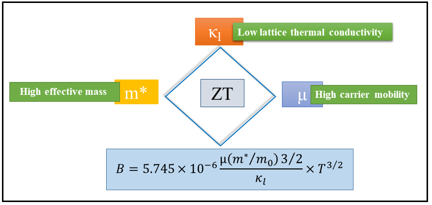
Figure 1: Schematic diagram for designing high performance TE materials. These strategies and concepts are used to maximize the thermoelectric figure of merit ZT value. Here B refer as a dimensionless material parameter

In this study we have focused on the principle of the Seebeck effect, which is used in many areas of research, such as in the automotive industry to increase fuel efficiency, in power plants to convert waste heat to electricity, to convert solar heat to electricity and in radioisotope TE generators for space probes. TE materials have low maintenance, long life cycle, and high reliability, which make possible to use them on Earth, in space, and deep in the ocean. TE materials can be used from low to high temperature applications such as electronic circuits/microchips (portable cooling) and radioactive TE generators which are mainly used by the National Aeronautics and Space Administration (NASA). Though there are many advantages in using TE materials, there is also some disadvantages such as high thermal conductivity, poor electrical conductivity, and low Seebeck coefficient those will reduces the ZT value, i.e heat to energy conversion efficiency. The main focus in the TE research society is to optimize the ZT value by reducing the thermal conductivity. The three main strategies used by scientists to reduce the thermal conductivity of the lattice to increase the ZT values are alloying, introducing complex crystal structures, and nanoengineering Joshi et al. (2011); Kanatzidis (2009); Pei et al. (2011a); Xie et al. (2010); Poudeu et al. (2009); Joshi et al. (2008); Liu et al. (2012a); Alam and Ramakrishna (2013).

Alloying method works on the strategy of phonon glass and electron crystal (PGEC) behavior Slack (1995). The PGEC suggests an ideal state in which the phonon should see the material as amorphous with a large number of phonon scattering center and the electron should see the material as a crystalline structure with minimal electron scattering. In this method, one can introduce defects by introducing two or more atoms on the same sites of the system, thus changing the crystal structure and achieving high ZT value by reducing the lattice thermal conductivity. The idea of the second strategy, i.e complex crystal structure, is to make the optical phonon mode flat, which increases the Umklapp scattering Toberer et al. (2011) and thus decreases the thermal conductivity. This intensifies the search for new bulk TE with complex unit cell to discover new phases such as clathrates Cohn et al. (1999), skutterudites Nolas et al. (1998); Caillat et al. (1996) and complex Zintl phases Toberer et al. (2009); Kauzlarich et al. (2007); Toberer et al. (2010). In recent years, new developments in nanostructure materials have attracted much interest in the TE community to develop new thermoelectric nanomaterials with high power factor (PF) and high ZT value due to the enhanced density of states (DOS) near Fermi level via quantum confinement. The thermal conductivity due to phonons can be suppressed in nanostructures in order to get better electrical conductivity and ZT Zhang et al. (2010); Hicks and Dresselhaus (1993); Venkatasubramanian et al. (2001); Xie et al. (2009). Band structure calculations show that the half$-$Heusler (HH) alloys with 18 VEC are narrow band semiconductors Kuentzler et al. (1992); Tobola et al. (1998), resulting in high Seebeck coefficient and large effective mass. Isoelectronic substitution, i.e the substitution of elements from the same group of The Periodic Table in TE materials, is well known and has attracted much attention for reducing thermal conductivity. The substitution of two or more atoms of different size and mass introduce more phonon scattering centers into the system via mass fluctuation Ren et al. (2020). This substitution approach has been adopted by many research groups to develop new multinary TE compounds. Figure. 1 shows some of the strategies and approaches proposed by many researchers to maximize the ZT value. A dimensionless material parameter B, which is directly related to the ratio between the effective mass of charge carriers and the mass of free electron charge, carrier mobility, temperature and inversely related to the thermal conductivity of the lattice at a given temperature, is also considered for achieving the maximum ZT value. Considering these material parameters one can design high efficiency TE materials with high ZT value. One can achieve the heavier effective mass, high carrier mobility and increase in phonon scattering by well$-$known strategies such as band convergence, band alignment, alloying and nanostructuring.

In the 1950s, Ioffe Ioffe (1957) suggested that alloying (forming solid solutions) was an effective way to optimize the TE performance. Alloying technique is widely used in chalcogenides, silicides, selenides, zintl phases, and HH compounds  Jaldurgam et al. (2021) But, selecting effective alloying elements to reduce the lattice thermal conductivity is a great challenge for the researcher due to the fact that alloying reduces the value of lattice thermal conductivity while it also reduces the charge carrier mobility. Wang et al. Wang et al. (2013) proposed that elements with heavy mass and small alloying scattering potential reduce the lattice thermal conductivity without greatly affecting the charge carrier mobility. Furthermore, it was found that the alloying atoms with heavier mass and smaller radius difference from the host atoms is the most reasonable choice to reduce the lattice thermal conductivity. To achieve high TE conversion efficiency, one must achieve high ZT value Zhu et al. (2015); Bulman and Cook (2014). One of the most common strategies to achieve this is to reduce the total thermal conductivity, which consists of both electronic and lattice parts (i.e. $\kappa$ $=$ $\kappa_{e}+\kappa_{L}$). Most work focuses on reducing the lattice portion of the thermal conductivity to increase the TE performance Xie et al. (2014); Kutorasinski et al. (2014); Chaput et al. (2006). One of the widely used approaches to reduce the lattice thermal conductivity in HH alloys is to introduce mass/stress fluctuation effect by isoelectronic or aliovalent doping/substitution. Experimental studies also show that the multinary compounds can be formed with more than 5 or more elements while maintaining the semiconducting behaviour in these systems Xie et al. (2013); Lee and Chao (2010); Simonson et al. (2011); Xie et al. (2012, 2008); Sekimoto et al. (2007).

The mass and size differences between the host atoms and the substituted atoms create point defects that scatter more phonons and thus reduce the lattice thermal conductivity Yang et al. (2004). Numerous studies show that doping at Ti site of TiNiSn or TiCoSb can effectively reduce the lattice thermal conductivity Sakurada and Shutoh (2005); Yan et al. (2013). However, the maximum ZT value achieved for doped/substituted TiNiSn is still in the range of 0.3$-$0.6 only Katayama et al. (2003); Gelbstein et al. (2011); Birkel et al. (2012); Douglas et al. (2012) so far due to the high lattice thermal conductivity. The recent study by Gürthet al. Gürth et al. (2016) showed that they have achieved a ZT value of 0.98 for TiNiSn by using a modified preparation route. In addition, they also achieved ZT value of 1.2 for multi$-$component systems. It was found that the Hf atom is an effective dopant at the Ti site that lowers the thermal conductivity of the lattice Fu et al. (2015). In this work, despite the traditional isoelectronic substitution approach, we report our recent progress in aliovalent substitution by substituting III^rd (Sc, Y, La) IV^th (Ti, Zr, Hf) and V^th (V, Nb, Ta) group elements at the Ti site of TiNiSn. To model the pentanary systems, we have substituted 25% of the III^rd, 50% of the IV^th and 25% of the V^th group elements at the Ti sites of TiNiSn. These aliovalent substitutions are chosen in such a way that the total number of VEC is always 18 to preserve the semiconducting behavior (see Table 1). For simplicity, we divide these systems into Sc, Y and La series. This article is divided into the following parts. The first part contains the methodology to compute the structural and the transport properties of these pentanary systems. The second part involve results and analysis and that is presented in two parts where the first part is the analysis of the electronic structure and the second part is a brief description of the TE transport properties including lattice dynamics of some of the selected systems, which could be considered as potential candidates for high$-$efficiency TE materials. The last section is the conclusions.

II Computational Details

Density functional theory (DFT) calculations for structural optimization and the electronic structure calculations were performed using projector$-$augmented plane$-$wave (PAW) Kresse and Joubert (1999) method, as implemented in the Vienna ab initio simulation package (VASP) Kresse and Furthmüller (1996). For the exchange$-$correlation potential in all our calculations we have used the generalized gradient approximation (GGA) Perdew et al. (1996) proposed by Perdew$-$Burke$-$Ernzerh. The Brillouin zone (BZ) was sampled using a Monkhorst Pack scheme Monkhorst and Pack (1976) for structural optimization and employed a 12$\times$12$\times$8 k$-$mesh. A plane$-$wave energy cutoff of 600 eV is used for geometry optimization for all the pentanary substituted TiNiSn. The convergence criterion for energy was taken to be 10^-6 eV/cell for total energy minimization and that for the Hellmann$-$Feynman force acting on each atom was taken less than 1 meV/Å  for ionic relaxation. We have used the tetrahedron method with Blöchl correction Blöchl et al. (1994) for BZ integrations for calcuating the density of states. Our previous study shows that the computational parameters used for the present study are sufficient enough to accurately predict the equilibrium structural parameter for HH alloys Choudhary and Ravindran (2020).

The full potential linearized augmented plane wave method as implemented in WIEN2k code Blaha et al. (2001); Schwarz and Blaha (2003) was used for calculating the accurate band structure for TE transport properties calculations. We have used a very high density of k$-$point 31$\times$31$\times$31 with R_MTK_max $=$ 7, where R_MT is the smallest atomic sphere radii of all the atomic spheres and K_max represent the maximum reciprocal lattice vector in the plane wave expansion and the convergence criteria is set to be 1 mRy/cell for all our calculations in order to obtain accurate eigenvalue. We have then used the calculated eigen energy in the BoltZTraP code Madsen and Singh (2006) for calculating the TE transport properties such as Seeback coefficient, electrical conductivity, and the electronic part of the thermal conductivity. For calculating the lattice dynamic properties a finite displacement method implemented in the VASP$-$Phonopy Togo and Tanaka (2015) interface was used with supercell approach. In all the phonon calculations we have used relaxed primitive cells to create supercell of dimension 2$\times$2$\times$2 with the displacement distance of 0.01 Å. The third order anharmonic force constants were calculated using VASP$-$Phono3py Togo et al. (2015) with a 2$\times$2$\times$2 supercell incorporating interactions out to 5th nearest neighbors. Finally, we calculated lattice thermal conductivity by explicitly solving the phonon Boltzmann transport equation.

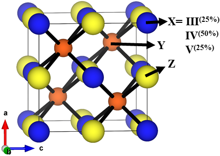
Figure 2: The conventional unit cell of half$-$Heusler alloy TiNiSn (XYZ). The pentanary substituted TiNiSn is modeled by substituting the III^rd, IV^th and V^th group atoms with the composition of 25%, 50% and 25% at Ti site of TiNiSn, respectively.

III Results and Discussion

III.1 Structural Description

The electronic structure of full Heusler Kübler et al. (1983) (FH) and HH Pierre et al. (1997); Tobo  l a and Pierre (2000); Offernes et al. (2007) alloys are vary with the VEC. Their properties can easily be predicted by counting their valence electrons Graf et al. (2011). The HH alloys can be described by the general formula XYZ with a composition 1:1:1 and they crystallize in a non$-$centrosymmetric cubic structure with space group F$\bar{4}$3m (no.216), while the FH alloys are generally described by the formula X₂YZ with a composition of 2:1:1 and those crystallize in the cubic space group Fm$\bar{3}$m (no. 225). In these compounds the X and Y are transition metals or rare earth elements and Z is usually a main group element. The FH alloys show all kinds of multi$-$functional magnetic properties, such as magnetocaloric Krenke et al. (2005); Levin et al. (2017); Liu et al. (2012b), magneto$-$optical Buschow and Van Engen (1981); Picozzi et al. (2006); Sanvito et al. (2017) and half metallic ferromagnetic Kundu et al. (2017); Blum et al. (2009); Wurmehl et al. (2006) behaviors. The half metallic ferromagnet shows semiconducting behavior for electrons of one spin orientation while metallic for electrons with the opposite spin. The emerging new physical properties such as thermoelectricity Huang et al. (2018); Krishnaveni et al. (2016); Yang et al. (2008); Gofryk et al. (2011), superconductivity Radmanesh et al. (2018); Pavlosiuk et al. (2016); Xu et al. (2014); Pan et al. (2013); Nakajima et al. (2015), magnetic ordering Pavlosiuk et al. (2018); Suzuki et al. (2016) and topological transitions Manna et al. (2018); Shi et al. (2018); Liu et al. (2016); Xiao et al. (2010) of HH alloys have attracted more attention.

Figure. 2 shows the crystal structure of TiNiSn with four formula units, where the atom X is located at 4a (0 0 0), the Y atom is located at 4b ($\dfrac{1}{2}$, $\dfrac{1}{2}$, $\dfrac{1}{2}$) and the Z atom is located at 4c ($\dfrac{1}{4}$, $\dfrac{1}{4}$, $\dfrac{1}{4}$) position, respectively. The most electropositive element X in XYZ transfers its electron to the more electronegative elements Y and Z forming a closed shell configuration, i.e., d¹⁰ for Y and s²p⁶ for Z. Therefore, the HH alloys with 18 VEC are considered as non$-$magnetic and semiconducting alloys Jung et al. (2000). The structural analysis of the pentanary substitution show that the symmetry of the HH alloys reduces from cubic to tetragonal by pentanary alloying. The primitive unit cell of all pentanary substituted TiNiSn contains 12 atoms and has a tetragonal structure with space group P$\bar{4}$2m (No.111). The optimized equilibrium lattice parameters, heat of formation ($\Delta$H_f) and PBE$-$GGA band gap values for the pentanary substituted TiNiSn systems are summarized in Table 2. Also, our lattice dynamics calculations (discussed latter) for all these pentanary systems show no negative phonon mode indicating the thermodynamic stability of these systems.

Group				Composition	Ti	Ni	Sn
IIIrd	IVth	Vth		III0.25IV0.5 V0.25
Sc	Ti	V	ScTiV	ScZrV	ScHfV	✓	✓
	Zr	Nb	ScTiNb	ScZrNb	ScHfNb	✓	✓
	Hf	Ta	ScTiTa	ScZrTa	ScHfTa	✓	✓
Y	Ti	V	YTiV	YZrV	YHfV	✓	✓
	Zr	Nb	YTiNb	YZrNb	YHfNb	✓	✓
	Hf	Ta	YTiTa	YZrTa	YHfTa	✓	✓
La	Ti	V	LaTiV	LaZrV	LaHfV	✓	✓
	Zr	Nb	LaTiNb	LaZrNb	LaHfNb	✓	✓
	Hf	Ta	LaTiTa	LaZrTa	LaHfTa	✓	✓

Table 1: The list of predicted pentanary HH alloys formed from the combination of the III^rd, IV^th and V^th group atoms with the composition of 25%, 50% and 25% at the Ti site of TiNiSn, respectively.

Table 2:  The structural parameters for transition metals substituted at Ti site in TiNiSn where Z=1; A, B, C, D, E, F and G are in the Wyckoff position 1a (0, 0, 0), 2f (0, 1/2, 1/2), 1d (1/2, 1/2 0), 4n (x${}^{{}^{\prime}}$, y${}^{{}^{\prime}}$, z${}^{{}^{\prime}}$) 2e(1/2, 0, 0), 1b (1/2, 1/2, 1/2) and 1c (0, 0, 1/2). The lattice parameters a and c (in Å), the internal structure parameter (z) obtained from our structural optimization, PBE$-$GGA band gap value E_g (in eV), heat of formation ($\Delta$H_f) (in kJ mol^-1 are listed. All the pentanary substituted systems have space group P$\bar{42}$m (No.111).

Compound	Unit$-$cell dimension (Å)			Positional parameters			$\Delta$Hf (kJ mol-1)	Eg (eV)
	a	c		x${}^{{}^{\prime}}$	y${}^{{}^{\prime}}$	z${}^{{}^{\prime}}$
TiNiSn	5.94	5.94					$-$56.02	0.45
La0.25Ti0.5V0.25NiSn	6.108	6.118		0.735	0.735	0.256	$-$53.91	0.21
La0.25Zr0.5V0.25NiSn	6.204	6.217		0.732	0.732	0.247	$-$60.66	0.17
La0.25Hf0.5V0.25NiSn	6.178	6.189		0.735	0.735	0.251	$-$58.04	0.27
La0.25Ti0.5Nb0.25NiSn	6.141	6.154		0.738	0.738	0.26	$-$54.30	0.20
La0.25Zr0.5Nb0.25NiSn	6.230	6.244		0.735	0.735	0.252	$-$60.86	0.22
La0.25Hf0.5Nb0.25NiSn	6.206	6.221		0.736	0.736	0.255	$-$58.25	0.23
La0.25Ti0.5Ta0.25NiSn	6.134	6.145		0.736	0.736	0.257	$-$55.27	0.24
La0.25Zr0.5Ta0.25NiSn	6.224	6.236		0.734	0.734	0.249	$-$61.92	0.28
La0.25Hf0.5Ta0.25NiSn	6.201	6.213		0.734	0.734	0.252	$-$59.31	0.32

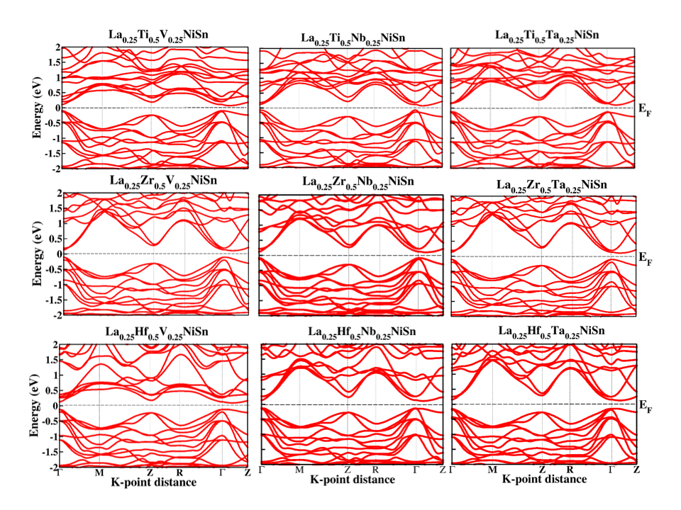
Figure 3: The calculated band structures for pentanary systems La_0.25X${}^{IV}_{0.5}$X${}^{V}_{0.25}$NiSn where (X^IV $=$ Ti, Zr and Hf, and X^V $=$ V, Nb and Ta) substituted at Ti site in TiNiSn obtained from PBE$-$GGA calculation.

III.2 Analysis of the electronic structure of pentanary substituted TiNiSn.

The good TE materials are considered to have a small band gap value. However, there is no set of rules to determine the exact band gap value to optimize the ZT. This, of course gives us the freedom to design efficient TE by modifying their band structures including band gap values, band edge positions, and carrier mobilities. Band offset and band convergence Hao et al. (2019); Lee et al. (2020); Xiao and Zhao (2018); Zhu et al. (2018) play an important role in TE materials for the design of n$-$type or p$-$type materials and their effect on the TE properties. These aspects were investigated by comparing the contributions of the light and heavy conduction bands to the electrical resistance and Seebeck coefficient. The pentanary substitution is made under the assumption of a rigid band approximation, where the shape of the DOS curve is not going to change by the substitution and there is only a shift in the Fermi level due to the electron/hole doping if we vary the VEC to analyse the role of electron/hole doping/substitution on the transport properties. However, a large atomic size mismatch between Zr, Hf and V enhances the TE transport properties, which will be discussed in the next section of this paper.

The concept of multiband model to describe the TE properties was first introduced by Simon Simon (1964) in late 1964. He showed very clearly the relationship between the maximization of the dimensionless material parameter ZT value by focusing on the two$-$band model. The two$-$band model, i.e., a conduction band (CB) and a valence band (VB), was considered a very effective approach to tune the Fermi energy, which is a function of the DOS, the effective mass of the charge carriers, the temperature and the optimal doping conditions (donors and acceptors). Later, Slack et al Slack and Hussain (1991), liu et al Liu et al. (2008) and pei et al Pei et al. (2011b) predicted the maximum energy conversion efficiency by utilizing three band model.

Figure. 3 shows the calculated electronic band structures obtained with the PBE$-$GGA function for La_0.25X${}^{IV}_{0.5}$X${}^{V}_{0.25}$NiSn where (X^IV $=$ Ti, Zr and Hf, and X^V $=$ V, Nb and Ta) series close to their band edge, i.e., from $-$2 eV to 2 eV. The band structure is plotted along the high symmetry directions of the first BZ of the simple tetragonal lattice for these pentanary substituted systems. Our PBE$-$GGA calculations show that all these systems possess semiconducting behavior with the band gap values varying from 0.17 to 0.32 eV. Also, all these materials show indirect band gap behavior with the valence band maximum (VBM) at the $\Gamma$ point and the conduction band minimum (CBM) between the $\Gamma$ to Z points.

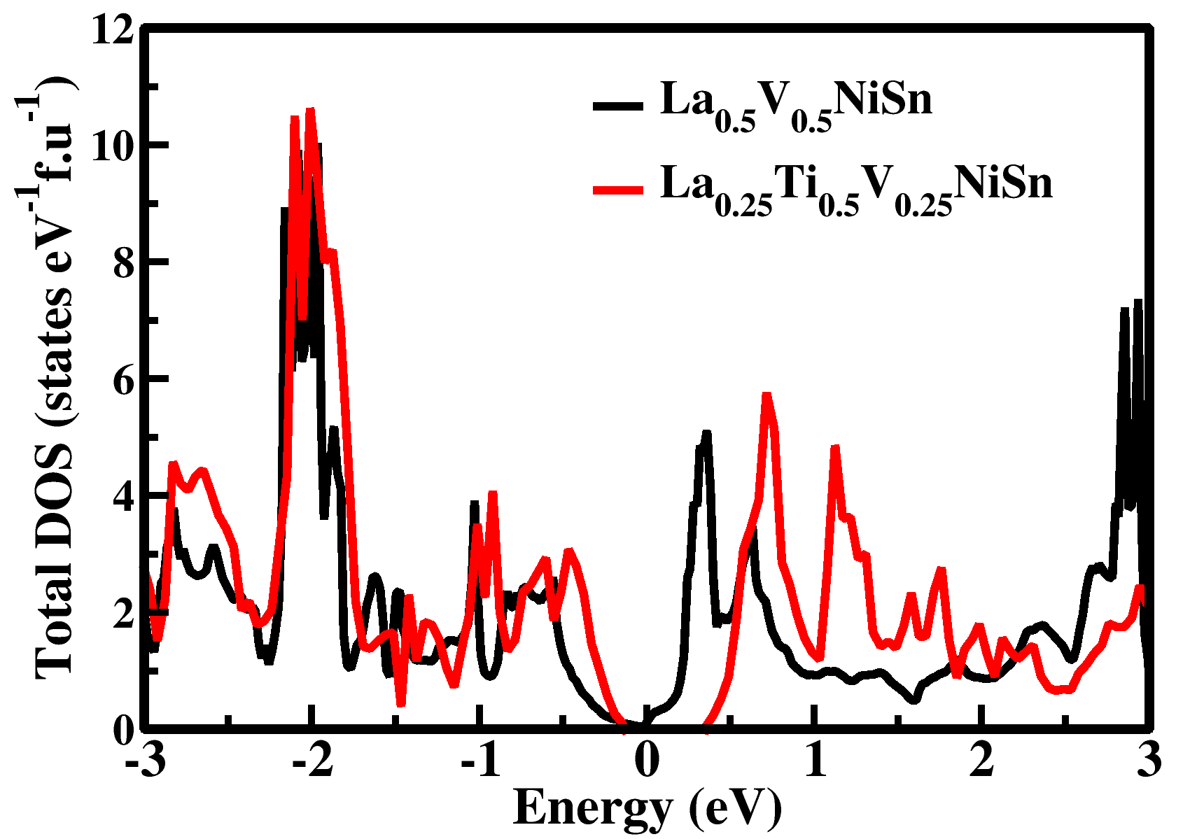
Figure 4: The calculated total density of states for the quaternary (La_0.25V_0.25NiSn) and pentanary (La_0.25Ti_0.5V_0.25NiSn) obtained from PBE$-$GGA calculation.

In our previous study Choudhary and Ravindran (2020), it was found that the quaternary systems with (La, V)_0.5, (La, Nb)_0.5, and (La, Ta)_0.5 substituted at the Ti site in TiNiSn exhibit semi$-$metallic behavior. In this work, we show that a semiconducting state can be achieved by inserting additional atoms from the IV^th group element of The Periodic Table in the Ti sites of TiNiSn i.e La_0.25X${}^{IV}_{0.5}$X${}^{V}_{0.25}$NiSn. The introduction of this additional transition metal atoms increases the hybridization between the d$-$ and p$-$orbitals resulting a band gap opening. Further, the electrons donated by these additional electropositive elements stabilizes the system by filling up the bonding states and opening the band gap between the VB and CB states. A broad comparison is needed here to show the differences in the electronic structure between these systems. In the case of La_0.25X${}^{IV}_{0.5}$V_0.25NiSn where (X^IV $=$ Ti, Zr, Hf) series, the band gap increases upon substitution of Ti with Zr or Hf. The calculated band gap values for La_0.25Ti_0.5V_0.25NiSn, La_0.25Zr_0.5V_0.25NiSn, and La_0.25Hf_0.5V_0.25NiSn, are 0.17, 0.2, and 0.21 eV, respectively. Similarly, the band gap values increase in the case of La_0.25X${}^{IV}_{0.5}$Nb_0.25NiSn with the order of 0.2, 0.22 and 0.23 eV, and for La_0.25X${}^{IV}_{0.5}$Ta_0.25NiSn 0.24, 0.28 and 0.32 eV, when X^IV $=$ Ti, Zr, Hf), respectively.

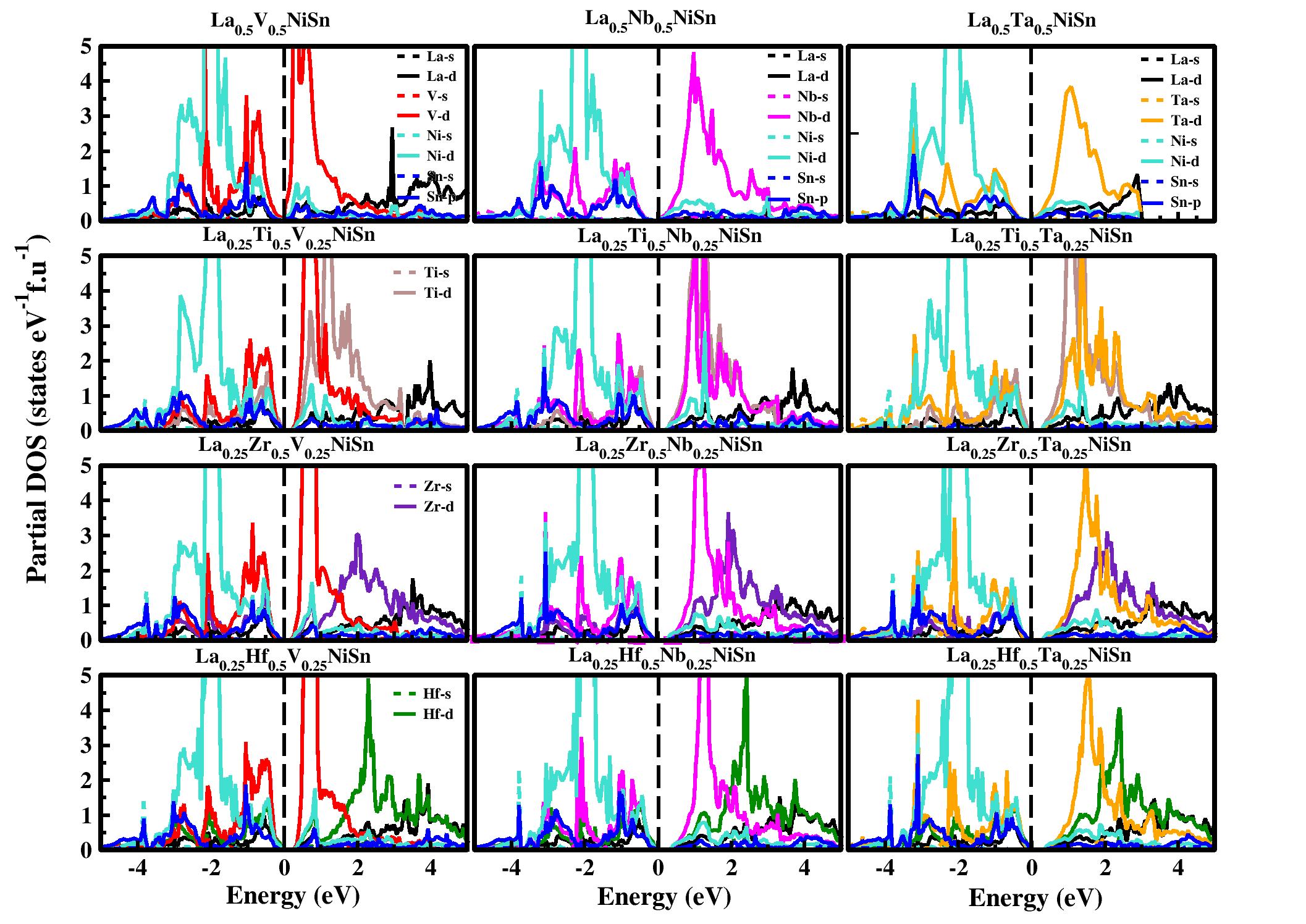
Figure 5: The calculated partial density of states for the pentanary La_0.25X${}^{IV}_{0.5}$X${}^{V}_{0.25}$NiSn where (X^IV $=$ Ti, Zr and Hf, and X^V $=$ V, Nb and Ta) substituted at the Ti site in TiNiSn obtained from PBE$-$GGA calculation.

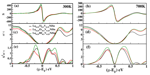
Figure 6: The calculated transport properties (a) and (b) Seebeck coefficient (in $\mu$V/K) , (c) (d) electrical conductivity (in 10¹⁹/$\Omega$ms) and (e) and (f) power factor (in 10¹¹W/mK²s ) as a function of chemical potential $\mu$ in the range of $-$1 to 1 eV at 300 and 700 K obtained from PBE$-$GGA calculation.

There is a cluster of narrow bands around $-$2 eV, in the band diagram in Fig. 3 and are originating from the Ni$-$3d electrons and they show sharp peak in the VB in the DOS curve. Reasonably dispersed bands present in the VBM are equally contributed by all the five atoms in all the pentanary compounds considered in the present study. The electronic band structure of all these systems have several adjacent low$-$lying bands (LLB) around the CBM and are get degenerate at the $\Gamma$ point in all these compounds as shown in Fig. 3. Though these materials are having indirect band feature, the energy difference between the direct bandgap and the indirect band gap is very small. Hence, though these materials are having indirect band behavior, the energy loss due to phonon assisted optical excitation will be very small. The lowest conduction band disperses rapidly from the $\Gamma$ point and flattens out as it approaches the Z point, giving rise to the high effective electron mass. The electronic band structure of all the pentanary substituted TiNiSn has small band gap values compared to TiNiSn, which is also responsible for enhancing the ZT.

In order to understand the role of pentanary addition in introducing the semiconducting behaviour we have plotted the total DOS for the quaternary La_0.25V_0.25NiSn and pentanary La_0.25Ti_0.5V_0.25NiSn systems and are shown in Fig. 4. From the total DOS analysis we can see that the addition of extra atom shift the CBM in to high energy region and open up the band gap. On the other hand, the quaternary system show the semi$-$metallic behaviour. If one go from quaternary to pentanary substituted systems i.e. La_0.5V_0.5NiSn to (La_0.25Zr_0.5V_0.25NiSn), our electronic structure calculation predict that a band gap is open up. For example, the substitution of Ti, Zr and Hf as a donors lead to an expected upward shift of the CBM.

To understand the contribution of electronic states responsible for the electronic transport, we have calculated the partial DOS for La_0.25X${}^{IV}_{0.5}$X${}^{V}_{0.25}$NiSn and are displayed in Figure. 5. The detail analysis of the partial DOS curve of La_0.25X${}^{IV}_{0.5}$V_0.25NiSn where (X^IV $=$ Ti, Zr, Hf) show that the d$-$states of all the four transition metals and Sn$-$p states are equally contributing to the VBM. However, the CBM is mainly contributed equally by V, Ni, and Ti$-$d states with small contribution from both La$-$d and Sn$-$p states equally. If we replace Ti with Zr or Hf then the d$-$states from these atoms systematically shifted to higher energy in the CB and this could explain why the band gap increases when the Ti is replaced with Zr or Hf in these pentanary systems. However, in all these systems the contribution from the La$-$d and the Sn$-$p states to the VBM is very small compared with the electronic d$-$states contributed by the other three transition metals. Though the Ni$-$d electrons are mainly localized around $-$2 eV in the VB its contribution at the band edges are almost same as the contribution from thed$-$states of V/Nb/Ta. While the V^th group elements (V, Nb and Ta)$-$d states show the main contribution in CM between the energy range of 0.5$-$2.5 eV, and are also responsible for the semi$-$metallic nature in La_0.5X_0.5NiSn (X$=$V, Nb, Ta) systems. From these analysis one can conclude that the hole transport in these systems are equally contributed by all the five atoms. However, the electron transport is dominated by the d$-$states of Ti/Zr/Hf and V/Nb/Ta with moderate contribution from Ni$-$d states and small contribution equally by the La$-$d and Sn$-$p states. It may be noted that the contribution from the s$-$ states of the constituents are negligibly small in both VBM and CBM and hence these electrons will not participate significantly in the transport properties of these systems.

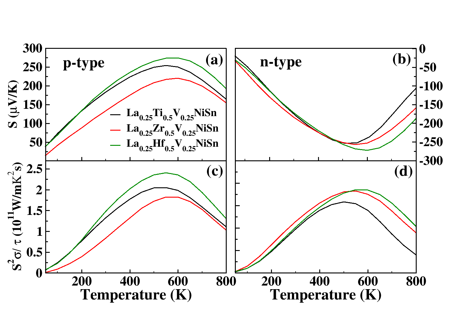
Figure 7: The temperature dependent transport properties at the optimal doping carrier concentrations under p$-$type and n$-$type conditions (a) and (b) Seebeck coefficient (S) and (c) and (d) power factor (${S^{2}\sigma}$) obtained from PBE$-$GGA functional calculation.

III.3 Thermoelectric transport properties

For metals or degenerate semiconductors Seebeck coefficient and electrical conductivity are given by the equation

$$S=\frac{8\pi^{2}k^{2}_{B}}{3eh^{2}}\Big{(}\frac{\pi}{3n}\Big{)}^{2/3}m^{*}T$$ (2)

$$\sigma=\frac{ne^{2}\tau}{m^{*}}$$ (3)

where k_B, h, e, T, n, and m^∗, $\sigma$ and $\tau$ are the Boltzmann constant, Planck constant, electrical charge, absolute temperature, carrier concentration, carrier effective mass, electrical conductivity and averaged relaxation time of electron, respectively. Seebeck coefficient and electrical conductivity are inversely proportional to each other, also these quantities are strongly dependent on temperature and chemical potential. With the increase of doping concentration and temperature, the electrical conductivity increases and Seebeck coefficient decreases. To maximize the PF, one needs to increase both $S$ and $\sigma$.

Fig. 6. shows the $S$, $\sigma$/$\tau$ and PF (${S^{2}\sigma}$/$\tau$) for La_0.25X${}^{IV}_{0.5}$V_0.25NiSn where (X^IV $=$ Ti, Zr, Hf) as a function of chemical potential in the interval range of $\mu-E_{F}=\pm$1 eV at two constant temperatures 300 K, and 700 K. From the Fig. 6. (a) and (b), one can see that the Seebeck coefficient decrease as the Fermi level shifts down towards the VB or shifts up towards the CB with hole/electron doping. It can be seen that at 300 K and 700 K, the Seebeck coefficient exhibits two peaks, one corresponds to p$-$type and other corresponds to n$-$type conditions. We can also see that these peaks are much closer to the VBM and CBM. It can be seen that at 300 K, the maximum values of Seebeck coefficients are 423.82, 352.23 and 473.92 $\mu$V/K at $\mu-E_{F}=$ $-$0.037, $-$0.044 and $-$0.046 eV in p$-$type condition and $-$349.32, $-$377.95 and $-$435.85 $\mu$V/K at $\mu-E_{F}=$ 0.040, 0.041 and 0.044 eV in n$-$type condition for La_0.25Ti_0.5V_0.25NiSn, La_0.25Zr_0.5V_0.25NiSn, and La_0.25Hf_0.5V_0.25NiSn, respectively. However, at higher temperature ( 700 K) the peak values decreases to 235.08, 210.26 and 255.77 $\mu$V/K at $\mu-E_{F}=$ $-$ 0.098, $-$0.095 and $-$0.097 eV in p$-$type and $-$224.13, $-$232.27 and $-$257.22 $\mu$V/K at $\mu-E_{F}=$ 0.091, 0.086 and 0.081 eV in n$-$type condition, respectively for the above mentioned compounds. In general, the Seebeck coefficient in HH compounds starts decreasing with increase of temperature and this is due to the fact that at higher temperatures the charge carrier hole/electron conductivity increases with the increase of thermal energy. Figure. 6 (c) and (d), show the electrical conductivity per relaxation time ($\sigma$/$\tau$) as a function of chemical potential. There are two peaks in these curves, one corresponds to p$-$type and other corresponds to n$-$type conditions. The maximum electrical conductivity in p$-$type and n$-$type conditions for La_0.25Ti_0.5V_0.25NiSn, La_0.25Zr_0.5V_0.25NiSn, and La_0.25Hf_0.5V_0.25NiSn are 11.53, 10.87 and 9.95 10¹⁹/$\Omega$ms at $\mu-E_{F}=$ $-$1, $-$0.92 and $-$1 eV and 8.97, 10.75 and 10.5 10¹⁹/${\Omega}$ms at $\mu-E_{F}=$ 0.54, 0.56 and 0.55 eV at 300 K, respectively. Whereas, the highest value of $\sigma$/$\tau$ at 700 K in p$-$type and n$-$type conditions for La_0.25Ti_0.5V_0.25NiSn, La_0.25Zr_0.5V_0.25NiSn, and La_0.25Hf_0.5V_0.25NiSn are 11.24, 10.69 and 10.23 10¹⁹/$\Omega$ms at $\mu-E_{F}=$ $-$1 eV and 7.83, 9.95 and 10.14 10¹⁹/${\Omega}$ms at $\mu-E_{F}=$ 1 eV, respectively. However, one can see that the electrical conductivity is less affected by temperature compared to Seebeck coefficient. Moreover, we have noticed that the electrical conductivity of all the investigated compounds is relatively low at low chemical potential at 300 K compared to 700 K and it increases rapidly with the increase of chemical potential since the electrical conductivity is directly proportional to charge carrier density.

Let us now discuss about the power factor (${S^{2}\sigma}$/$\tau$) which is an important parameter for searching the high efficiency TE materials. Figure. 6. (e) and (f), shows the calculated PF for La_0.25X${}^{IV}_{0.5}$V_0.25NiSn where (X^IV $=$ Ti, Zr, Hf). From the Fig. 6. (e) and (f) one can see that the calculated PF for all the selected compounds are lower value at 300 K. and reach high value at higher temperature i.e at 700 K. For example, at 300 K one can see the shift in the chemical potential for all the investigated compounds with respect to the maximum PF. In the case of p$-$type condition, the maximum PF for La_0.25Ti_0.5V_0.25NiSn, La_0.25Zr_0.5V_0.25NiSn, and La_0.25Hf_0.5V_0.25NiSn are 1.45, 1.20 and 1.81 10¹¹W/mK²s at $\mu-E_{F}=$ $-$0.19, $-$0.28 and $-$0.22 eV, respectively. The highest PF at low value of chemical potential for La_0.25Ti_0.5V_0.25NiSn indicating that one can maximize the PF by small hole doping. However, for La_0.25Zr_0.5V_0.25NiSn, and La_0.25Hf_0.5V_0.25NiS one need to do heavy hole doping to maximize the PF. In the case of n$-$type condition, for all these three compounds, the maximum value of PF achieved are 1.47, 1.41 and 1.5 10¹¹W/mK²s at $\mu-E_{F}=$ 0.21, 0.19 and 0.4 eV, respectively. At higher temperature i.e at 700 K the PF has almost doubled for all the investigated compounds compared to that at 300 K and the maximum PF for La_0.25Ti_0.5V_0.25NiSn, La_0.25Zr_0.5V_0.25NiSn, and La_0.25Hf_0.5V_0.25NiSn in p$-$type condition are 4.02, 3.97 and 4.61 10¹¹W/mK²s at $\mu-E_{F}=$ $-$0.21,$-$0.23 and $-$0.24) and in n$-$types condition are 4.22, 4.32 and 4.91 10¹¹W/mk²s at $\mu-E_{F}=$ 0.23, 0.26 and 0.29 eV), respectively.

Figure. 7 shows the temperature dependence TE transport properties at the fixed charge carrier concentration n $=$ 10²⁰ cm^-3 for both hole$-$doped and electron$-$doped (p$-$type and n$-$type) for La_0.25X${}^{IV}_{0.5}$V_0.25NiSn where (X^IV $=$ Ti, Zr, Hf). Figure. 7 (a) and (b) show the $S$ for the selected systems. The positive and negative values of $S$ indicate that holes/electrons are the dominant charge carriers, suggesting p$-$type and n$-$type condition. It can be seen that Seebeck coefficient increases rapidly with temperature and it reaches a maximum value at 550 k for all the investigated compounds and then decreases at higher temperature. The calculated Seebeck coefficient values for La_0.25Ti_0.5V_0.25NiSn, La_0.25Zr_0.5V_0.25NiSn, and La_0.25Hf_0.5V_0.25NiSn in p$-$type and n$-$type conditions are 253.54, 219.14 and 273.53 and -258.82, -256.84 and -268.57 $\mu$V/K at 550 k respectively. In both p$-$type and n$-$type condition La_0.25Hf_0.5V_0.25NiSn shows the maximum Seebeck coefficient value of 273.53 and -268.57 $\mu$V/k at 550 K. Figure.7 (c) and (d), shows the calculated power factor. It follows the similar trend as Seebeck coefficient i.e the power factor increases with temperature and reaches maximum value at 550 k and then decreases at higher temperature. The PF for La_0.25Hf_0.5V_0.25NiSn exhibits the highest pick for the p$-$type condition and the has maximum value of 2.44 10¹¹W/mk²s at 550 K.

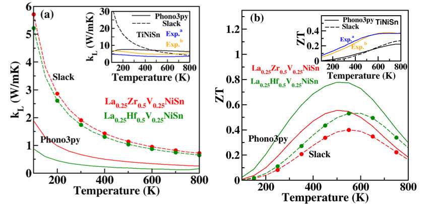
Figure 8: The comparison of calculated (a) lattice thermal conductivity ($\kappa_{L}$) and (b) thermoelectric figure of merit (ZT) between ternary (TiNiSn) and pentanary (La_0.25Zr_0.5V_0.25NiSn and La_0.25Hf_0.5V_0.25NiSn), half Heusler alloys as a function of temperature obtained from PBE$-$GGA functional calculation. The inset figures show the calculated and the available experimental $\kappa_{L}$ and ZT values for TiNiSn ( Exp.^a Birkel et al. (2013) Exp.^b Kim et al. (2007)).

Table 3: The calculated single crystal elastic constants C_ij (in GPa), the bulk modulus (B in GPa), shear modulus (G in GPa), Young modulus (E in GPa), longitudinal, transverse, average elastic wave velocity ($\nu$_l ,$\nu$_t,$\nu$_m in m/s), the Debye $\theta_{D}$ (in K) and acoustic Debye $\theta_{a}$ (in K) temperature, primitive unit cell volume (V in (ų)), average mass per atom $\overline{M_{a}}$ (in amu), Poisson’s ratio ($\nu$) and Grüneisen parameter ($\gamma$) for TiNiSn, La_0.25Zr_0.5V_0.25NiSn and La_0.25Hf_0.5V_0.25NiSn systems obtained from PBE$-$GGA calculation.

Parameters	TiNiSn	La0.25Zr0.5V0.25NiSn	La0.25Hf0.5V0.25NiSn
C11	238.09	216.31	220.29
C12	82.39	56.82	60.10
C13		59.21	62.30
C33		217.75	222.60
C44	64.30	46.86	47.30
C66		37.64	40.30
B	134.29	117.17	114.73
G	69.42	55.39	56.52
E	177.65	142.50	145.64
$\nu$l	5618.45	7627.20	7041.41
$\nu$t	3108.03	4173.71	3840.42
$\nu$m	3462.74	4653.93	4283.36
V	52.05	239.33	236.30
$\nu$	0.279	0.286	0.288
$\gamma$	1.64	1.68	1.7
$\overline{M_{a}}$	75.09	91.69	109.14
$\theta_{D}$	398.22	381.6	352.71
$\theta_{a}$	277.12	168.06	155.34

Table 4: The Calculated values of lattice thermal conductivity ($\kappa_{L}$ in W/mK) obtained from phonon dispersion curve (Phono3py) obtained from elastic constants (Slack’s equation) and the corresponding thermoelectric figure of merit ZT$-$Phono3py and ZT$-$Slack, respectively.

Compound	$\kappa_{L}-$Phono3py	$\kappa_{L}-$Slack	ZT$-$Phono3py	ZT$-$Slack
	300 K      550 K	300 K       550 K	300 K       550 K	300 K       550 K
TiNiSn	7.54       6.87	11.04      6.02	0.05       0.15	0.03       0.16
La0.25Zr0.5V0.25NiSn	0.66       0.37	1.91       1.04	0.29       0.54	0.14       0.40
La0.25Hf0.5V0.25NiSn	0.31       0.16	1.74       0.95	0.48       0.77	0.19       0.53

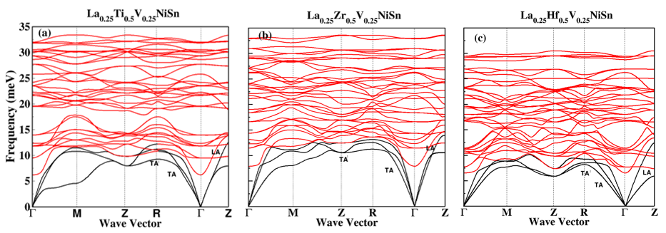
Figure 9: The calculated phonon dispersion curves for selected pentanary substituted systems such as La_0.25Ti_0.5V_0.25NiSn, La_0.25Zr_0.5V_0.25NiSn and La_0.25Hf_0.5V_0.25NiSn obtained from finite difference methods and are shown in (a), (b) and (c), respectively along the high symmetry lines. The optical and acoustic modes are highlighted with red and black colour, respectively

.

III.4 Lattice thermal conductivity and Thermoelectric figure of merit

Thermal conductivity plays an important role to study the behavior of the atom within a crystal lattice when it is heated or cooled. The low or high thermal conductivity of the materials are very useful to use them in wide range of applications to achieve the best performance of the systems. Therefore it is necessary to investigate the thermal conductivity of the materials as an important parameter for designing new materials. The DFT calculation of thermal conductivity is computationally expensive and time consuming. In the 19^th century Debye Debye (1912) proposed the concept of phonon which is the lattice vibration of the solid crystal. In his work he used the quantized normal mode of atomic vibrations to explain the specific heat capacity of the crystalline solids. The concept of phonon provide a new way to describe the lattice vibration of the solids from which many thermodynamic properties can be calculated like lattice thermal conductivity, Debye temperature, Güneisen parameter, specific heat capacity, and lattice thermal expansion. Peierls  Peierls (1955); Ziman (1960) was among the first to use the idea of Boltzmann transport theory (BTE) for calculating the lattice phonon life times and lattice thermal conductivity. Since then, solving BTE is considered as a best method for accurately predicting the $\kappa_{L}$ Broido et al. (2007); Ward and Broido (2010); Tang and Dong (2010). But, solving the BTE is a complicated task. Therefore to solve the complex set of equations a variety of approximation have thus been used for understanding the phonon driven thermal properties Callaway (1959); Allen (2013); Deinzer et al. (2003). Nowadays with more computational power and open source code such as Phono3py  Togo et al. (2015), PhonTS Chernatynskiy and Phillpot (2015), almaBTE  Tadano et al. (2014) and ShengBTE Li et al. (2014) one can perform the ab initio calculations to solve the BTE from the third order anharmonic force constant for calculating the $\kappa_{L}$. However, calculation of third order interatomic force constant is time$-$consuming and computationally expensive. The simplest method or formula was developed by Slack Slack and Hussain (1991) for calculating the $\kappa_{L}$ by measuring the speed of sound which carry the energy of phonon and anharmonicity in term of Debye temperature and average Grüneisen parameter, which is given as

$$\kappa_{L}=A\dfrac{\overline{M_{a}}\delta\theta\textsubscript{a}^{3}}{\gamma^{2}Tn^{2/3}}$$ (4)

where $\overline{M_{a}}$ is the average mass per atom in the crystal, $\theta_{a}$ is the acoustic Debye temperature, $\delta$ is the cube root of the average volume per atom, $n$ is the number of atoms in the primitive unit cell, $\gamma$ is the Grüneisen parameter. and $A$ is a physical quantity which can be calculated as A$=\dfrac{2.43\times 10^{-8}}{1-0.514/\gamma+0.228/\gamma^{2}}$ The bulk modulus (B) and shear modulus (G) are obtained from the Voigt$-$Reuss$-$Hill$-$(VRH) theory as

$$B_{v}=1/9(C_{11}+C_{22}+C_{33})+2/9(C_{12}+C_{23}+C_{13})$$ (5)

$$\begin{split}G_{V}&=1/15(C_{11}+C_{22}+C_{33})-1/15(C_{12}+C_{23}+C_{13})\\ &+1/5(C_{44}+C_{55}+C_{66})\end{split}$$ (6)

$$1/B_{R}=(S_{11}+S_{22}+S_{33})+2(S_{12}+S_{23}+S_{13})$$ (7)

$$\begin{split}1/G_{R}&=4/15(S_{11}+S_{22}+S_{33})-4/15(S_{12}+S_{23}+S_{13})\\ &+1/5(S_{44}+S_{55}+S_{66})\end{split}$$ (8)

here the compliance constants S_ij is the inverse matrix of the single crystal elastic constant C_ij. Finally the B and G are obtained by averaging the B_V and B_R, G_V and G_R.

$$B=\frac{B_{V}+B_{R}}{2}$$ (9)

$$G=\frac{G_{V}+G_{R}}{2}$$ (10)

The Young’s modulus (E) and the Poisson’s ratio ($\nu$) were calculated as follows

$$E=\frac{9BG}{3B+G}$$ (11)

$$\nu=\frac{3B-2G}{6B+2G}$$ (12)

Furthermore the transverse (v_t) , longitudinal (v_l) and average (v_m) sound velocities are calculated by the following equations

$$v_{t}=\sqrt{\dfrac{E}{2\rho(1+\nu)}}=\sqrt{\frac{G}{\rho}}$$ (13)

$$v_{l}=\dfrac{E(1-\nu)}{\rho(1+\nu)(1-2\nu)}=\sqrt{(\frac{3B+4G}{3\rho})}$$ (14)

$$v_{m}=\sqrt{[\frac{1}{3}(\frac{2}{v\textsubscript{t}\textsuperscript{3}}+\frac{1}{v\textsubscript{l}\textsuperscript{3}})]}$$ (15)

here $\rho$ is the density of the material.

From the calculated v_t, v_l and v_m using the above approach one can calculate the Grüneisen parameter ($\gamma$), Debye temperature ($\theta_{D}$) and acoustic Debye temperature ($\theta_{a}$) by the following equations

$$\gamma=\dfrac{9-12(v\textsubscript{t}/v\textsubscript{l})^{2}}{2+4(v\textsubscript{t}/v\textsubscript{l})^{2}}$$ (16)

$$\theta\textsubscript{D}=\frac{h}{k}[\frac{3n}{4\pi}(\frac{N\textsubscript{A}\rho}{M})]\textsuperscript{1/3}v\textsubscript{m}$$ (17)

$$\theta\textsubscript{a}=\theta\textsubscript{D}n^{-1/3}$$ (18)

These parameters are easily calculated from the elastic properties such as bulk and shear moduli. The elastic constants and moduli can reveal the important thermal and lattice dynamic properties such as mechanical stability and chemical nature of the solids. The elastic constants C_ij are calculated from the strain$-$stress relationship Kachanov et al. (2003). From the Voigt$-$Reuss$-$Hill (VRH) theory  Den Toonder et al. (1999). one can calculate the elastic properties, such as bulk and shear modulus from the elastic constants. Table. 2 shows the calculated elastic constants C_ij and elastic moduli. From the calculated C_ij it is found that all the currently investigated compounds in the present study are mechanically stable as they obey the Cauchy$-$Born rule Ericksen (1984); Born (1940) about the stability criteria for the cubic and tetragonal structures. The calculated elastic constants and moduli show an increasing trend as Ti is substituted with the La/V, Hf or Zr in the TiNiSn system. The Hf substituted TiNiSn have large value of elastic constants and moduli and hence exhibit superior mechanical properties compared to other substituted systems. The calculated bulk modulus, shear modulus, Young’s modulus and Poisson’s ratio are listed in Table. 2.

Finally the lattice thermal conductivity is calculated from Slack’s equation using the Debye temperature and Grüneisen parameter calculated from elastic moduli such as B and G. (see Fig. 8. (a)). We have also calculated the $\kappa_{L}$ from the phonon band structure using Phono3py code. Fig. 8. (a) shows the comparison between the calculated $\kappa_{L}$ from Phono3py using phonon dispersion and Slack’s equation using the calculated elastic constants. From the Fig. 8. (a) we can see that at lower temperatures i.e below 300 K the difference between the calculated $\kappa_{L}$ values from Slack and Phono3py are larger than the values at higher temperature for parent TiNiSn and the pentanary systems. However at higher temperatures we observed smaller difference between them. In the case of TiNiSn (see the inset Fig. 8. (a) the difference between the $\kappa_{L}$ values obtained from these two approaches is very small and it overlap at 500 K. The calculated $\kappa_{L}$ value for TiNiSn from the phonon dispersion relation and Slack’s approach are 6.87 and 6.02 W/mK at 550 K. Also we observed that our calculated $\kappa_{L}$ value for TiNiSn from Phono3py code is well matched with the reported experimental studies Bhattacharya et al. (2002); Katayama et al. (2003); Downie et al. (2013).

From the Fig. 8. (a) we observed that the multinary substituted systems have lower $\kappa_{L}$ values than those from the parent TiNiSn as we have expected due to increase in phonon scattering. In the case of La_0.25Zr_0.5V_0.25NiSn and La_0.25Hf_0.5V_0.25NiSn the calculated $\kappa_{L}$ from Slack’s equation at 300 K are 1.91 and 1.74 W/mK, respectively. However, the calculated $\kappa_{L}$ value from phonon dispersion curve for these compounds are much smaller (only 0.66 and 0.31 W/mK, respectively) than that from Slack’s approach. It may be noted that our calculated lattice thermal conductivity from both the methods follows the same trend i.e reduces with increase of temperature. The La_0.25Hf_0.5V_0.25NiSn system shows small value of $\kappa_{L}$ and this can be understood from the difference in Debye temperature, Grüneisen parameter. The La_0.25Hf_0.5V_0.25NiSn has low value of Debye temperature and high value of Grüneisen parameter which is favorable for low $\kappa_{L}$.

The ZT of parent and the pentanary systems are evaluated by substituting the corresponding calculated value of S, $\sigma$, T, $\kappa_{e}$ and the $\kappa_{L}$ into the ZT equation 1. Figure. 8. (b) shows the calculated ZT value as a function of temperature. We have also calculated the ZT value by including the $\kappa_{L}$ calculated from Slack’s equation and from phonon dispersion relation using the Phono3py code. From the Fig. 8. (b) one can see that the ZT value for TiNiSn calculated from both the methods increases with temperature and reaches maximum value at around 800 K. Also at 500 K the ZT values obtained based on $\kappa_{L}$ values obtained from both the approach overlap with each other which follow the same trend as $\kappa_{L}$ . The calculated ZT for TiNiSn including $\kappa_{L}$ value calculated from Slack and Phono3py are 0.27 and 0.22 at 800 K, respectively. In the case of La_0.25Zr_0.5V_0.25NiSn and La_0.25Hf_0.5V_0.25NiSn we find the ZT value increases with temperature and reaches maximum value at 550 K and then reduces at higher temperatures. We can observe the significant difference in the ZT values calculated from both the methods. The calculated ZT value for La_0.25Zr_0.5V_0.25NiSn from Slack’s equation and from phonon dispersion relation using the Phono3py code are 0.54 and 0.4 at 550 K, respectively. However, the difference between the ZT values obtained from these two approaches are minimum at 800 K. In the case of La_0.25Hf_0.5V_0.25NiSn also we found the same trend in the ZT as La_0.25Zr_0.5V_0.25NiSn and the calculated values for ZT from these two approaches are 0.77 and 0.53 at 550 K, respectively.

We have also compared our calculated $\kappa_{L}$ and ZT values with the available experimental results (see inset figure in Fig. 8. (a)) and (b), respectively. Our calculated $\kappa_{L}$ from phonon dispersion relation using the Phono3py code shows slightly larger value as compared to experiment. However, the $\kappa_{L}$ calculated from Slack’s approach shows the large difference at lower temperature (below 300 K), but shows very good agreement at high temperature (above 400 K). However, the experimentally estimated $\kappa_{L}$ values are found in the range between 2.4$-$6.08 W/mK. Our reported $\kappa_{L}$ provide reasonable agreement with the reported experimental studies. The experimentally estimated ZT show the little large value compared with our ZT calculated from phonon dispersion relation using the Phono3py code and Slack’s equation. The discrepancy between the theoretical and experimental calculated $\kappa_{L}$ and ZT may be attributed to the fact that the theoretical results are applicable to defect free single crystal and experimetally synthesised samples are usually poly crytal with various defects that could influence the transport properties. Moreover, synthesizing the pure TiNiSn is very challenging, small amounts of impurity phases and interstitial Ni defects change the majority and minority charge carrier concentration and therefore the TE transport properties Douglas et al. (2012); Kirievsky et al. (2013); Berche and Jund (2018); Young and Reddy (2019). Unfortunately there are no experimental investigations on the TE properties of La_0.25Zr_0.5V_0.25NiSn and La_0.25Hf_0.5V_0.25NiSn to compare with the present results. Therefore, we hope that there will be more theoretical and experimental work on these materials in future to develop high efficiency TE materials based on HH alloys.

III.5 Lattice dynamic calculation of pentanary substituted TiNiSn

The thermodynamic properties of selected systems are calculated with the Phonopy and Phono3py codes using the finite displacement and supercell approach. The generation of the supercell structures with displacements are made using the Phonopy code. The supercell structure contains the information about the atomic displacements, then the forces acting on the atoms corresponding to each displacement set are calculated by VASP code. All the force sets calculated by VASP code are then used to calculate the force constants. The dynamical matrix is built from the force constants and from the matrix one can generate the phonon frequencies and eigen vectors. Figure. 9 shows the phonon band structure for some of the selected pentanary systems.

The phonon dispersion curves are plotted along the high symmetry direction in the first BZ. The number of vibrational modes of the system depends on the number of atoms present in the unit cell. The 12 atoms present in the selected systems gives a total of 36 phonon branches, including one longitudinal acoustic (LA) mode, two transverse acoustic (TA) modes, and 33 optical modes. From the phonon dispersion curves shown in Fig. 9. (a), (b) and (c) for La_0.25X${}^{IV}_{0.5}$V_0.25NiSn where (X^IV $=$ Ti, Zr, Hf), it can be seen that for all these selected pentanary systems both the acoustic and optical bands are well mixed. By comparing the shape of the acoustic and optical bands of these systems we found that there is a frequency shift from La_0.25Ti_0.5V_0.25NiSn to La_0.25Hf_0.5V_0.25NiSn and this is due to the mass difference between the Ti, Zr and Hf atoms.

In the case of La_0.25Zr_0.5V_0.25NiSn and La_0.25Hf_0.5V_0.25NiSn we can find a strong optical$-$acoustic band mixing and therefore these systems are expected to have more optical$-$acoustic phonon$-$phonon scattering. We have also noticed the frequency shift towards lower energy for the Hf containing system in our calculated phonon dispersion curves compared to that of Ti and Zr containing systems. To know the contribution of various atoms to the heat capacity (C_v) we have calculated the heat capacity at constant volume (C_v). Figure. 10. shows the (C_v) at temperatures from 0 to 500 K, for all selected systems. The calculated C_v values for La_0.25Ti_0.5V_0.25NiSn, La_0.25Zr_0.5V_0.25NiSn and La_0.25Hf_0.5V_0.25NiSn at 100 K are 15.2, 15.9 and 17.25 $(J.K^{-1}.mol^{-1})$, respectively. The shift in frequency towards lower frequency in the phonon band structure for La_0.25Hf_0.5V_0.25NiSn over Ti or Zr containing system is due to the large average atomic mass in this system that results in higher C_v value compared to the other systems.

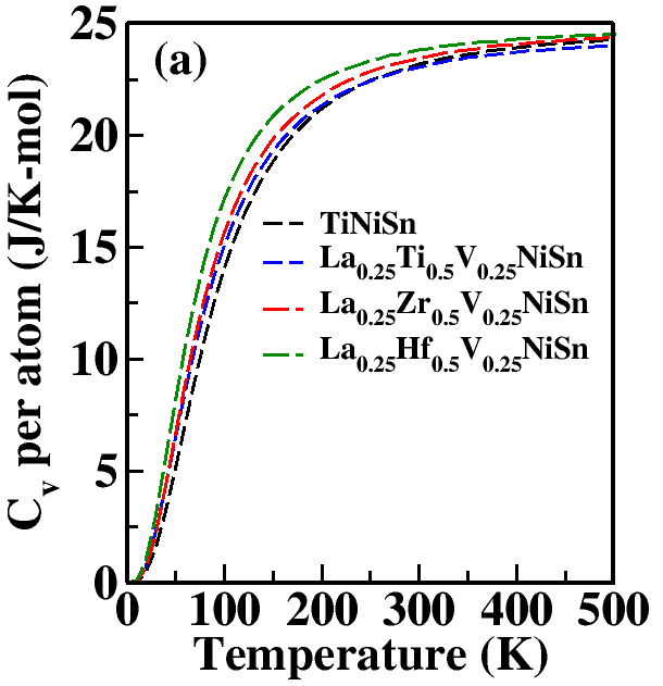
Figure 10: The calculated heat capacity as a function of temperature for pure, quaternary and pentanary substituted TiNiSn series.

IV Conclusion

This work focuses on designing the new series of pentanary substituted TiNiSn HH alloys with the aliovalent substitution retaining the 18 valence electrons count using VASP$-$PAW method and studied the electronic structure of nine pentanary systems. The thermoelectric transport properties have been studied by combining Boltzmann transport theory with the electronic structure obtained from full potential Wien2k code. Our calculated band structure analysis shows that all pentanary substituted TiNiSn systems has semiconducting behavior and small band gap compared to pure TiNiSn. The calculated band gap values for the pentanary systems in the present work ranges from 0.17 to 0.32 eV. The calculated lattice part of thermal conductivity $\kappa_{L}$ using finite difference method implemented in the Phono3py code and the calculated elastic constants with Slack’s equation show good agreement at high temperatures. From the calculated $\kappa_{L}$ we show that the pentanary substituted systems have a lower value compared to pure TiNiSn due to mass fluctuation. Moreover, we have obtained comparable $\kappa_{L}$ values from Phono3py code and Slack’s equation for the pentanary systems La_0.25Hf_0.5V_0.25NiSn and La_0.25Zr_0.5V_0.25NiSn which are found to be 0.37 (1.04) and 0.16 (0.95) W/mK at 550 K, respectively and the corresponding maximum ZT value are found to be 0.54 (0.4) and 0.77 (0.53) at 550 K, respectively. These results show that the pentanary substituted TiNiSn is an excellent example where we can increase the ZT value by lowering the band gap through electronic band structure engineering thus increase electrical conductivity and decrease the thermal conductivity by mass fluctuation. The improved thermoelectric efficiency in these pentanary based systems suggests a novel means to further improve thermoelectric performance through band engineering and lowering the thermal conductivity by multinary addition thus plays an important role in the development of efficient TE materials for high efficiency TE devices.

References

- Bell (2008) L. E. Bell, Science 321, 1457 (2008).
- Jaumot (1958) F. E. Jaumot, Proceedings of the IRE 46, 538 (1958).
- Zhao and Tan (2014) D. Zhao and G. Tan, Applied Thermal Engineering 66, 15 (2014).
- Joshi et al. (2011) G. Joshi, X. Yan, H. Wang, W. Liu, G. Chen, and Z. Ren, Advanced Energy Materials 1, 643 (2011).
- Kanatzidis (2009) M. G. Kanatzidis, Chemistry of materials 22, 648 (2009).
- Pei et al. (2011a) Y. Pei, J. Lensch-Falk, E. S. Toberer, D. L. Medlin, and G. J. Snyder, Advanced Functional Materials 21, 241 (2011a).
- Xie et al. (2010) W. Xie, J. He, H. J. Kang, X. Tang, S. Zhu, M. Laver, S. Wang, J. R. Copley, C. M. Brown, Q. Zhang, et al., Nano letters 10, 3283 (2010).
- Poudeu et al. (2009) P. F. Poudeu, A. Guéguen, C.-I. Wu, T. Hogan, and M. G. Kanatzidis, Chemistry of materials 22, 1046 (2009).
- Joshi et al. (2008) G. Joshi, H. Lee, Y. Lan, X. Wang, G. Zhu, D. Wang, R. W. Gould, D. C. Cuff, M. Y. Tang, M. S. Dresselhaus, et al., Nano letters 8, 4670 (2008).
- Liu et al. (2012a) W. Liu, X. Yan, G. Chen, and Z. Ren, Nano Energy 1, 42 (2012a).
- Alam and Ramakrishna (2013) H. Alam and S. Ramakrishna, Nano energy 2, 190 (2013).
- Slack (1995) G. A. Slack, CRC handbook of thermoelectrics , 407 (1995).
- Toberer et al. (2011) E. S. Toberer, A. Zevalkink, and G. J. Snyder, Journal of Materials Chemistry 21, 15843 (2011).
- Cohn et al. (1999) J. Cohn, G. Nolas, V. Fessatidis, T. Metcalf, and G. Slack, Physical Review Letters 82, 779 (1999).
- Nolas et al. (1998) G. Nolas, J. Cohn, and G. Slack, Physical Review B 58, 164 (1998).
- Caillat et al. (1996) T. Caillat, A. Borshchevsky, and J.-P. Fleurial, Journal of Applied Physics 80, 4442 (1996).
- Toberer et al. (2009) E. S. Toberer, A. F. May, and G. J. Snyder, Chemistry of Materials 22, 624 (2009).
- Kauzlarich et al. (2007) S. M. Kauzlarich, S. R. Brown, and G. J. Snyder, Dalton Transactions , 2099 (2007).
- Toberer et al. (2010) E. S. Toberer, A. F. May, B. C. Melot, E. Flage-Larsen, and G. J. Snyder, Dalton transactions 39, 1046 (2010).
- Zhang et al. (2010) G. Zhang, Q. Yu, W. Wang, and X. Li, Advanced Materials 22, 1959 (2010).
- Hicks and Dresselhaus (1993) L. D. Hicks and M. S. Dresselhaus, Physical Review B 47, 12727 (1993).
- Venkatasubramanian et al. (2001) R. Venkatasubramanian, E. Siivola, T. Colpitts, and B. O’quinn, Nature 413, 597 (2001).
- Xie et al. (2009) W. Xie, X. Tang, Y. Yan, Q. Zhang, and T. M. Tritt, Journal of Applied Physics 105, 113713 (2009).
- Kuentzler et al. (1992) R. Kuentzler, R. Clad, G. Schmerber, and Y. Dossmann, Journal of Magnetism and Magnetic Materials 104, 1976 (1992).
- Tobola et al. (1998) J. Tobola, J. Pierre, S. Kaprzyk, R. Skolozdra, and M. Kouacou, Journal of Physics: Condensed Matter 10, 1013 (1998).
- Ren et al. (2020) Q. Ren, C. Fu, Q. Qiu, S. Dai, Z. Liu, T. Masuda, S. Asai, M. Hagihala, S. Lee, S. Torri, et al., Nature communications 11, 1 (2020).
- Ioffe (1957) A. F. Ioffe, Semiconductor Thermoelements, and (Info-search, Limited, 1957).
- Jaldurgam et al. (2021) F. F. Jaldurgam, Z. Ahmad, and F. Touati, Nanomaterials 11, 895 (2021).
- Wang et al. (2013) H. Wang, Y. Pei, A. D. LaLonde, and G. J. Snyder, in Thermoelectric Nanomaterials (Springer, 2013) pp. 3–32.
- Zhu et al. (2015) T. Zhu, C. Fu, H. Xie, Y. Liu, and X. Zhao, Advanced Energy Materials 5, 1500588 (2015).
- Bulman and Cook (2014) G. Bulman and B. Cook, in Energy Harvesting and Storage: Materials, Devices, and Applications V, Vol. 9115 (International Society for Optics and Photonics, 2014) p. 911507.
- Xie et al. (2014) H. Xie, H. Wang, C. Fu, Y. Liu, G. J. Snyder, X. Zhao, and T. Zhu, Scientific reports 4, 6888 (2014).
- Kutorasinski et al. (2014) K. Kutorasinski, J. Tobola, and S. Kaprzyk, physica status solidi (a) 211, 1229 (2014).
- Chaput et al. (2006) L. Chaput, J. Tobola, P. Pécheur, and H. Scherrer, Physical Review B 73, 045121 (2006).
- Xie et al. (2013) H. Xie, H. Wang, Y. Pei, C. Fu, X. Liu, G. J. Snyder, X. Zhao, and T. Zhu, Advanced Functional Materials 23, 5123 (2013).
- Lee and Chao (2010) P.-J. Lee and L.-S. Chao, Journal of Alloys and Compounds 504, 192 (2010).
- Simonson et al. (2011) J. Simonson, D. Wu, W. Xie, T. Tritt, and S. Poon, Physical Review B 83, 235211 (2011).
- Xie et al. (2012) W. Xie, A. Weidenkaff, X. Tang, Q. Zhang, J. Poon, and T. Tritt, Nanomaterials 2, 379 (2012).
- Xie et al. (2008) W. Xie, Q. Jin, and X. Tang, Journal of Applied Physics 103, 043711 (2008).
- Sekimoto et al. (2007) T. Sekimoto, K. Kurosaki, H. Muta, and S. Yamanaka, Japanese Journal of Applied Physics 46, L673 (2007).
- Yang et al. (2004) J. Yang, G. Meisner, and L. Chen, Applied physics letters 85, 1140 (2004).
- Sakurada and Shutoh (2005) S. Sakurada and N. Shutoh, Applied Physics Letters 86, 082105 (2005).
- Yan et al. (2013) X. Yan, W. Liu, S. Chen, H. Wang, Q. Zhang, G. Chen, and Z. Ren, Advanced Energy Materials 3, 1195 (2013).
- Katayama et al. (2003) T. Katayama, S. W. Kim, Y. Kimura, and Y. Mishima, Journal of electronic materials 32, 1160 (2003).
- Gelbstein et al. (2011) Y. Gelbstein, N. Tal, A. Yarmek, Y. Rosenberg, M. P. Dariel, S. Ouardi, B. Balke, C. Felser, and M. Köhne, Journal of Materials Research 26, 1919 (2011).
- Birkel et al. (2012) C. S. Birkel, W. G. Zeier, J. E. Douglas, B. R. Lettiere, C. E. Mills, G. Seward, A. Birkel, M. L. Snedaker, Y. Zhang, G. J. Snyder, et al., Chemistry of Materials 24, 2558 (2012).
- Douglas et al. (2012) J. E. Douglas, C. S. Birkel, M.-S. Miao, C. J. Torbet, G. D. Stucky, T. M. Pollock, and R. Seshadri, Applied Physics Letters 101, 183902 (2012).
- Gürth et al. (2016) M. Gürth, G. Rogl, V. Romaka, A. Grytsiv, E. Bauer, and P. Rogl, Acta Materialia 104, 210 (2016).
- Fu et al. (2015) C. Fu, S. Bai, Y. Liu, Y. Tang, L. Chen, X. Zhao, and T. Zhu, Nature communications 6, 1 (2015).
- Kresse and Joubert (1999) G. Kresse and D. Joubert, Phys. Rev. B 59, 1758 (1999).
- Kresse and Furthmüller (1996) G. Kresse and J. Furthmüller, Comput. Mater. Sci. 6, 15 (1996).
- Perdew et al. (1996) J. P. Perdew, K. Burke, and M. Ernzerhof, Phys. Rev. Lett 77, 3865 (1996).
- Monkhorst and Pack (1976) H. J. Monkhorst and J. D. Pack, Phys. Rev. B 13, 5188 (1976).
- Blöchl et al. (1994) P. E. Blöchl, O. Jepsen, and O. K. Andersen, Physical Review B 49, 16223 (1994).
- Choudhary and Ravindran (2020) M. K. Choudhary and P. Ravindran, Sustainable Energy & Fuels 4, 895 (2020).
- Blaha et al. (2001) P. Blaha, K. Schwarz, G. Madsen, D. Kvasnicka, and J. Luitz, Austria ISBN , 3 (2001).
- Schwarz and Blaha (2003) K. Schwarz and P. Blaha, Computational Materials Science 28, 259 (2003).
- Madsen and Singh (2006) G. K. Madsen and D. J. Singh, Computer Physics Communications 175, 67 (2006).
- Togo and Tanaka (2015) A. Togo and I. Tanaka, Scripta Materialia 108, 1 (2015).
- Togo et al. (2015) A. Togo, L. Chaput, and I. Tanaka, Physical Review B 91, 094306 (2015).
- Kübler et al. (1983) J. Kübler, A. William, and C. Sommers, Physical Review B 28, 1745 (1983).
- Pierre et al. (1997) J. Pierre, R. Skolozdra, J. Tobola, S. Kaprzyk, C. Hordequin, M. Kouacou, I. Karla, R. Currat, and E. Lelievre-Berna, Journal of alloys and compounds 262, 101 (1997).
- Tobo l a and Pierre (2000) J. Tobo l a and J. Pierre, Journal of alloys and compounds 296, 243 (2000).
- Offernes et al. (2007) L. Offernes, P. Ravindran, and A. Kjekshus, Journal of alloys and compounds 439, 37 (2007).
- Graf et al. (2011) T. Graf, C. Felser, and S. S. Parkin, Progress in solid state chemistry 39, 1 (2011).
- Krenke et al. (2005) T. Krenke, E. Duman, M. Acet, E. F. Wassermann, X. Moya, L. Mañosa, and A. Planes, Nature materials 4, 450 (2005).
- Levin et al. (2017) E. E. Levin, J. D. Bocarsly, K. E. Wyckoff, T. M. Pollock, and R. Seshadri, Physical Review Materials 1, 075003 (2017).
- Liu et al. (2012b) J. Liu, T. Gottschall, K. P. Skokov, J. D. Moore, and O. Gutfleisch, Nature materials 11, 620 (2012b).
- Buschow and Van Engen (1981) K. Buschow and P. Van Engen, Journal of Magnetism and Magnetic Materials 25, 90 (1981).
- Picozzi et al. (2006) S. Picozzi, A. Continenza, and A. J. Freeman, Journal of Physics D: Applied Physics 39, 851 (2006).
- Sanvito et al. (2017) S. Sanvito, C. Oses, J. Xue, A. Tiwari, M. Zic, T. Archer, P. Tozman, M. Venkatesan, M. Coey, and S. Curtarolo, Science advances 3, e1602241 (2017).
- Kundu et al. (2017) A. Kundu, S. Ghosh, R. Banerjee, S. Ghosh, and B. Sanyal, Scientific reports 7, 1 (2017).
- Blum et al. (2009) C. Blum, C. Jenkins, J. Barth, C. Felser, S. Wurmehl, G. Friemel, C. Hess, G. Behr, B. Büchner, A. Reller, et al., Applied Physics Letters 95, 161903 (2009).
- Wurmehl et al. (2006) S. Wurmehl, G. H. Fecher, H. C. Kandpal, V. Ksenofontov, C. Felser, and H.-J. Lin, Applied physics letters 88, 032503 (2006).
- Huang et al. (2018) S. Huang, X. Liu, W. Zheng, J. Guo, R. Xiong, Z. Wang, and J. Shi, Journal of Materials Chemistry A 6, 20069 (2018).
- Krishnaveni et al. (2016) S. Krishnaveni, M. Sundareswari, P. Deshmukh, S. Valluri, and K. Roberts, Journal of Materials Research 31, 1306 (2016).
- Yang et al. (2008) J. Yang, H. Li, T. Wu, W. Zhang, L. Chen, and J. Yang, Advanced Functional Materials 18, 2880 (2008).
- Gofryk et al. (2011) K. Gofryk, D. Kaczorowski, T. Plackowski, A. Leithe-Jasper, and Y. Grin, Physical Review B 84, 035208 (2011).
- Radmanesh et al. (2018) S. Radmanesh, C. Martin, Y. Zhu, X. Yin, H. Xiao, Z. Mao, and L. Spinu, Physical Review B 98, 241111 (2018).
- Pavlosiuk et al. (2016) O. Pavlosiuk, D. Kaczorowski, X. Fabreges, A. Gukasov, and P. Wiśniewski, Scientific reports 6, 18797 (2016).
- Xu et al. (2014) G. Xu, W. Wang, X. Zhang, Y. Du, E. Liu, S. Wang, G. Wu, Z. Liu, and X. X. Zhang, Scientific reports 4, 5709 (2014).
- Pan et al. (2013) Y. Pan, A. Nikitin, T. Bay, Y. Huang, C. Paulsen, B. Yan, and A. De Visser, EPL (Europhysics Letters) 104, 27001 (2013).
- Nakajima et al. (2015) Y. Nakajima, R. Hu, K. Kirshenbaum, A. Hughes, P. Syers, X. Wang, K. Wang, R. Wang, S. R. Saha, D. Pratt, et al., Science advances 1, e1500242 (2015).
- Pavlosiuk et al. (2018) O. Pavlosiuk, X. Fabreges, A. Gukasov, M. Meven, D. Kaczorowski, and P. Wi ’s niewski, Physica B: Condensed Matter 536, 56 (2018).
- Suzuki et al. (2016) T. Suzuki, R. Chisnell, A. Devarakonda, Y.-T. Liu, W. Feng, D. Xiao, J. W. Lynn, and J. Checkelsky, Nature Physics 12, 1119 (2016).
- Manna et al. (2018) K. Manna, Y. Sun, L. Muechler, J. Kübler, and C. Felser, Nature Reviews Materials 3, 244 (2018).
- Shi et al. (2018) F. Shi, L. Jia, M. Si, Z. Zhang, J. Xie, C. Xiao, D. Yang, H. Shi, and Q. Luo, Applied Physics Express 11, 095701 (2018).
- Liu et al. (2016) Z. Liu, L. Yang, S.-C. Wu, C. Shekhar, J. Jiang, H. Yang, Y. Zhang, S.-K. Mo, Z. Hussain, B. Yan, et al., Nature communications 7, 1 (2016).
- Xiao et al. (2010) D. Xiao, Y. Yao, W. Feng, J. Wen, W. Zhu, X.-Q. Chen, G. M. Stocks, and Z. Zhang, Physical review letters 105, 096404 (2010).
- Jung et al. (2000) D. Jung, H.-J. Koo, and M.-H. Whangbo, Journal of Molecular Structure: THEOCHEM 527, 113 (2000).
- Hao et al. (2019) S. Hao, V. P. Dravid, M. G. Kanatzidis, and C. Wolverton, npj Computational Materials 5, 58 (2019).
- Lee et al. (2020) K. H. Lee, S.-i. Kim, H.-S. Kim, and S. W. Kim, ACS Applied Energy Materials (2020).
- Xiao and Zhao (2018) Y. Xiao and L.-D. Zhao, npj Quantum Materials 3, 1 (2018).
- Zhu et al. (2018) H. Zhu, R. He, J. Mao, Q. Zhu, C. Li, J. Sun, W. Ren, Y. Wang, Z. Liu, Z. Tang, et al., Nature communications 9, 1 (2018).
- Simon (1964) R. Simon, Solid-State Electronics 7, 397 (1964).
- Slack and Hussain (1991) G. A. Slack and M. A. Hussain, Journal of applied physics 70, 2694 (1991).
- Liu et al. (2008) W.-S. Liu, L.-D. Zhao, B.-P. Zhang, H.-L. Zhang, and J.-F. Li, Applied Physics Letters 93, 042109 (2008).
- Pei et al. (2011b) Y. Pei, X. Shi, A. LaLonde, H. Wang, L. Chen, and G. J. Snyder, Nature 473, 66 (2011b).
- Birkel et al. (2013) C. S. Birkel, J. E. Douglas, B. R. Lettiere, G. Seward, N. Verma, Y. Zhang, T. M. Pollock, R. Seshadri, and G. D. Stucky, Physical Chemistry Chemical Physics 15, 6990 (2013).
- Kim et al. (2007) S.-W. Kim, Y. Kimura, and Y. Mishima, Intermetallics 15, 349 (2007).
- Debye (1912) P. Debye, Annalen der Physik 344, 789 (1912).
- Peierls (1955) R. Peierls, London, England , 108 (1955).
- Ziman (1960) J. Ziman, “Electrons and phonons, oxford university press,” (1960).
- Broido et al. (2007) D. A. Broido, M. Malorny, G. Birner, N. Mingo, and D. Stewart, Applied Physics Letters 91, 231922 (2007).
- Ward and Broido (2010) A. Ward and D. Broido, Physical Review B 81, 085205 (2010).
- Tang and Dong (2010) X. Tang and J. Dong, Proceedings of the National Academy of Sciences 107, 4539 (2010).
- Callaway (1959) J. Callaway, Physical Review 113, 1046 (1959).
- Allen (2013) P. B. Allen, Physical Review B 88, 144302 (2013).
- Deinzer et al. (2003) G. Deinzer, G. Birner, and D. Strauch, Physical Review B 67, 144304 (2003).
- Chernatynskiy and Phillpot (2015) A. Chernatynskiy and S. R. Phillpot, Computer Physics Communications 192, 196 (2015).
- Tadano et al. (2014) T. Tadano, Y. Gohda, and S. Tsuneyuki, Journal of Physics: Condensed Matter 26, 225402 (2014).
- Li et al. (2014) W. Li, J. Carrete, N. A. Katcho, and N. Mingo, Computer Physics Communications 185, 1747 (2014).
- Kachanov et al. (2003) M. L. Kachanov, B. Shafiro, and I. Tsukrov, Handbook of elasticity solutions (Springer Science & Business Media, 2003).
- Den Toonder et al. (1999) J. Den Toonder, J. Van Dommelen, and F. Baaijens, Modelling and Simulation in Materials Science and Engineering 7, 909 (1999).
- Ericksen (1984) J. Ericksen, The Cauchy and Born Hypotheses for Crystals. Academic Press, London , 61 (1984).
- Born (1940) M. Born, in Mathematical Proceedings of the Cambridge Philosophical Society, Vol. 36 (Cambridge University Press, 1940) pp. 160–172.
- Bhattacharya et al. (2002) S. Bhattacharya, T. M. Tritt, Y. Xia, V. Ponnambalam, S. Poon, and N. Thadhani, Applied physics letters 81, 43 (2002).
- Downie et al. (2013) R. A. Downie, D. MacLaren, R. Smith, and J. Bos, Chemical communications 49, 4184 (2013).
- Kirievsky et al. (2013) K. Kirievsky, Y. Gelbstein, and D. Fuks, Journal of Solid State Chemistry 203, 247 (2013).
- Berche and Jund (2018) A. Berche and P. Jund, Intermetallics 92, 62 (2018).
- Young and Reddy (2019) J. Young and R. Reddy, Journal of Materials Engineering and Performance 28, 5917 (2019).