Thin accretion disks around traversable wormholes

Abstract

In this paper, we aim to investigate various physical properties and characteristics of radiation emerging from the surface of accretion disks, in a rotating traversable axially symmetric wormhole spacetime of the Teo class. We have studied the marginally stable orbits and accretion efficiency graphically, corresponding to different values of dimensionless spin parameter $J/M^{2}$ ranging from 0.2 to 1.5 and some values of the throat radius $r_{0}$, in comparison to the Kerr black hole with the same parameter values, and also tabulated the results. The energy flux radiated by the accretion disk $F(r)$, the temperature distribution $T(r)$ and the emission spectra $\nu L(\nu)$ is plotted, corresponding to varying values of the dimensionless spin parameter $J/M^{2}$ and throat radius $r_{0}$. Also, the critical frequency at which the luminosity attains its maximum value, for various values of the angular momentum of the wormhole $J/M^{2}$ and $r_{0}$ is tabulated. Lastly, we have employed ray-tracing technique, to produce the intensity map of the image of an accretion disk, as observed by an asymptotic observer, under two conditions: firstly when the disk is on the same side as the observer and we have also compared those with the images of an accretion disk in case of Kerr black hole with same parameters. Secondly, the images have been provided when the disk and observer are on opposite sides of the throat. This study may help to detect and distinguish wormhole geometries from other compact objects.

I Introduction:

It is argued that the mass of almost all astrophysical bodies develop through accretion. The current observation of the center of the galaxy M87 through the Event Horizon Telescope suggests that in most of the active galactic nuclei (AGN’s), there exist gas clouds around the galactic center, together with an accompanying accretion disc. These gas clouds (scales from a tenth of a parsec to a few hundred parsecs ) are expected to develop a geometrically and optically distorted disc that engrosses maximum of the ultraviolet radiation and the soft X-rays. Significant astrophysical evidence can be obtained from the observation of the motion of the gas flows in the gravitational field of super massive objects. The temperature in the innermost region of the disk is about $10^{7}K$ and from this hot region, the X-ray emission arises. To study the strong field gravity, one can use these highly compact objects, as the detected emission arises from regions close to these compact objects. According to the standard theory, the accretion disk is presumed to be an optically thick Newtonian type. This model suggests that the local emergent flux ( just like a black body ) is associated with the energy decadence at a specific radial point in the disk. The sum of black body components coming from various radial positions in the disk yields the observed spectrum. Usually, general relativistic issues change this Newtonian spectrum by incorporating Doppler broadening, gravitational redshifts, and light bending.

Since wormholes kg1 , kg14 are a specific type of astrophysical objects, so it has been an active area of research to study accretion phenomenon around wormholes. The phenomenon of accretion around compact objects is an outstanding example for studying the signatures of wormholes versus black holes. Initial research on accretion disks using a Newtonian approach was conducted by Shakura and R.A. Sunyaev.SS Later Thorne et. al. first developed a general relativistic model of the thin accretion disk, where the accreting matter had a Keplerian motion. They assumed the disk is in a steady-state, i.e., the mass accretion rate $\dot{M}$ does not change with time, as well as it is independent of the radius of the disk. From a theoretical point of view, the efficient cooling due to radiation transport, maintains this disk in hydrodynamic and thermodynamic equilibrium, thus ensuring a black body electromagnetic spectrum. The spectra from the sources may provide some information on the geometry and dynamics of innermost regions of accretion disks. Following Page-Thorne Page model, one can study emissivity properties such as the luminosity spectra, flux of radiation, temperature profile using accretion around wormholes Luminet . Further radiation properties of thin accretion disks were analysed in Thorne ; Gair , along with the effects of the photon capture by the black hole on the spin evolution. The emissivity properties of the accretion disks, which helps us to study the conversion of rest mass into emitting radiation in the accretion disk were studied in Bhat , Torres , Yuan , Guzman . The work in these papers have helped to distinguish between the accretion properties around different classes of exotic central objects, such as non-rotating or rotating quark, boson or fermion star, by studying the radiation power per unit area, the temperature of the disk and the emission spectrum of the emitted radiation and comparing them with the Schwarzschild and Kerr black hole. Through the investigation of differences in the thermodynamic and electromagnetic properties of the accretion disks, Kovacs et. al. K , identified the observation signatures that may help to distinguish between black holes and naked singularities. Image of the Janis-Newman-Winicour naked singularity with a thin accretion disk was studied in Gyul . They concluded that for some specific values of the spin parameter and of the scalar charge, the radiation energy flux and conversion efficiency from the disk around a rotating naked singularity is higher than that around a Kerr black hole. Accretion around rotating wormholes is an active area of current research. Recently, gravitational wave echoes of the Damour-Solodukhin wormhole (RDSWH) have been studied by Bueno et al. Bueno . Nandi et.al. further studied a rotating generalization of the RDSWHNandi and concluded that RDSWH are experimentally indistinguishable from Kerr black hole by accretion characteristics. Similar works on comparative study of thin accretion disks around rotating gravastars and Kerr-type black holes, in order to distinguish between them, was undertaken byHarko2 . It was concluded that gravastars provide a less efficient mechanism for converting mass to radiation than black holes. Many major works in modified theories of gravity are also available in literature. The physical properties of a thin accretion disk in the static and spherically symmetric spacetime metric of vacuum $f(R)$ gravity was analysed in Pun . Thus astrophysical observations of the emission spectra from accretion disks may lead us to the possibility of directly testing modified gravity models. Several classes of static and rotating brane world black holes have been investigated in Pun2 , and compared with the general relativistic case. The thin accretion disk features in dynamical Chern-Simons modified gravity have been studied extensively in Harko3 and in Horava-Lifshitz gravity in Harko4 . An interesting work on thin accretion disk around a rotating Kerr-like black hole in Einstein-bumblebee gravity model has been done by Bumblebee . Research on the properties of the radiation emerging from the surface of the accretion disk around static and rotating axially symmetric wormhole geometries were conducted in Harko5 , Harko6 . In Paul numerically constructed images of thin accretion disks in rotating wormhole backgrounds, for the Kerr-like and the Teo class of wormholes was studied, and interestingly it showed that there are dramatic differences between accretion disk images in wormhole backgrounds, compared to black hole ones, owing to the fact that a wormhole can theoretically have accretion disks on both sides of its throat. Although, Paul gives a full explanation of using ray-tracing of a general Teo wormhole, they have considered specific forms of the metric functions in order to generate results and images. In our present work, we have not merely changed parameters, but have taken completely different forms of the metric functions, thereby giving a wormhole with completely different spacetime geometry or gravitational field within the Teo class. Therefore, within the Teo class, depending on the forms of the metric functions, we could have various wormholes with various spacetime geometries or gravitational field, provided the forms of the metric functions satisfy the conditions obtained by Teo. The observational signatures in these various cases in principle will be different. The specific example which we have considered is completely different from the one considered in Paul . Moreover, the focus of Paul was on constructing the images, whereas our focus was not only on the images but also on the other properties such as luminosity, critical frequency etc. We believe that the results presented in the paper will indeed be relevant in future observations for the reasons explained there.

The motivation of the study is as follows. It is well-known that, according to the Kerr Black Hole Hypothesis, the spacetime geometry around astrophysical compact objects is well described by the Kerr solution of General Relativity (GR). However, in modified gravity theories or in presence of quantum effect or exotic matter, one can expect deviation from the Kerr spacetime. Such deviations should be tested using observations. Therefore, it is astrophysically relevant to study various observational aspects of other possible geometries beside those of the Kerr solution. The motivation behind such studies is to see whether to what extent we can distinguish between a Kerr black hole and a deviated non-Kerr spacetime. In cases where differences in the observational signatures arise, we can distinguish a Kerr black hole from a non-Kerr geometry. However, in cases where differences do not arise, a non-Ker geometry mimics a Kerr black hole. In our work, we have studied a similar aspect by considering a wormhole and a Kerr black hole. Although in the literature, there are several wormhole spacetimes which are obtained as exact solutions of GR as well as other modified gravity theories, and matter for such wormholes are known, most of these wormholes are non-rotating solutions. This is due to difficulties associated in obtaining rotating solutions as exact solutions. Given this difficulty, researchers often consider rotating wormhole models which are not exact solutions of any gravity theory, but can be used in modelling horizonless compact objects. The motivation behind this latter approach is comparative studies between a black hole and a wormhole through their observational aspects. In other words, the objective in this case is not the matter on the RHS of the field equations, but to see whether and to what extent we could distinguish between a wormhole and a black hole or to test the Kerr Black Hole Hypothesis through observational aspects. The literature is replete with several such kind of approaches. In our work also, the motivation was to explore comparative studies between a wormhole and a black hole through observational signatures of accretion disks around them.

The paper is organized as follows: in section II we have described some physical properties of thin accretion disks, followed by the investigation of marginally stable circular orbits in section III. Next in section IV, we have studied the accretion disk properties of a rotating traversable wormhole of the Teo class in details. Following this, in section V, the images of an accretion disk around a wormhole is analysed as observed by an asymptotic observer whose location is taken first on the same side of the throat as the disk; and again on the side of the throat opposite to that of the disk. Lastly, in section VI we have mentioned some concluding remarks.

II Some physical properties of thin accretion disks

Usually, it is claimed that compact X-ray sources are binary systems. One is a normal star and the other is a highly compact object and former landfills material onto its latter companion. The majority of the standard models for this mass transfer suggest that the relocated material forms a thin disk around the highly compact objects. The viscous stresses handover angular momentum outside over the disk, causing the material to spiral steadily inward. Also, these viscous stresses, functioning against the disk’s differential rotation, warm the disk thus producing a large flux of X-rays. According to steady-state models, the disk accretion ( in which accreting material is interstellar gas and magnetic fields ) onto a highly compact object may happen in the nuclei of galaxies. The gravitational energy of the accreting material converts to heat and some parts of the heat transform into radiation. This radiation partly seeps out and chills the accretion disc. After receiving this radiation and analyzing its electromagnetic spectrum through radio, optical and X-ray telescopes , we get information about the disk as well as compact object surrounded by the disk. In the analysis of mass accretion, we adopt a geometrically thin accretion disk. In the thin accretion disk, the vertical size of the disk is insignificant compared to its horizontal extension i.e. most of the matter lies close to the radial plane. This means that the disk height $H$ ( described by the maximum half-thickness of the disk ), is considerably lesser than any characteristic radii $R$ of the disk, $\frac{H}{R}<<1$. Here, the vertical size in cylindrical coordinates $(r,\phi,z)$ defined along the z-axis is negligible, Also for this consideration, stress and dynamic friction in the disk generates heat that can be spread through the radiation above its surface. This cooling process confirms that the disk could be in hydrodynamical equilibrium and as a result, the mass accretion rate $\dot{M}$ in the disk does not change with time i.e. constant. Since the disk is steadied at hydrodynamic equilibrium, the pressure and vertical entropy gradient should be negligible. This thin disk has an inner edge defined by the marginally stable circular radius $r_{ms}$ and the accreting matter at higher radii has a Keplerian motion. This thin accretion disk supposition implies that spacetime metric components as well as the accretion particles move in Keplerian orbits around the compact objects with a rotational velocity, $\Omega=\frac{d\phi}{dt}$ and its specific energy E $\&$ specific angular momentum L depends only on the radii of the orbits i.e. on the radial coordinate. The accretion particles with the four-velocity $u_{\mu}$ form a disk and the disk has an averaged surface density $\Sigma$,

$$\Sigma=\int_{-H}^{H}<\rho_{0}>dz,$$ (1)

where $\rho_{0}$ is the density of rest mass and H is the disk height during the time $\Delta t$. Here, $<\rho_{0}>$ is defined as the averaged rest mass density in time $\Delta t$ with angle $2\pi$. The orbiting particles in the disk is modeled by an anisotropic fluid source which is given by,

$$T^{\mu\nu}=\rho_{0}u^{\mu}u^{\nu}+2u^{(\mu}q^{\nu)}+t^{\mu\nu},$$ (2)

where the energy flow vector $q_{\mu}$ and the stress tensor $t^{\mu\nu}$ are measured in the averaged rest-frame with $u_{\mu}q^{\mu}=0,~{}u_{\mu}t^{\mu\nu}=0.$ Here we neglect specific heat. Another characteristic of the disk structure is the torque which is given by,

$$W_{\phi}^{r}=\int_{-H}^{H}<t_{\phi}^{r}>dz,$$ (3)

with the averaged component $<t_{\phi}^{r}>$ in time $\Delta t$ with angle $2\pi$. The most significant physical measure recounting the disk is the radiation flux $F(r)$ over the disk surface that can be obtained from the time and orbital average of the energy flux vector as,

$$F(r)=<q^{z}>.$$ (4)

Using stress energy tensor of the disk $T^{\mu\nu}$, one can define the four-vectors of the energy and of the angular momentum flux in a local basis as,

$$-E^{\mu}=T^{\mu}_{\nu}\left(\frac{\partial}{\partial t}\right)^{\nu}~{}and~{}J^{\mu}=T^{\mu}_{\nu}\left(\frac{\partial}{\partial\phi}\right)^{\nu},$$ (5)

respectively.

Now, the structure equations of the thin disk could be obtained from the conservation laws of the rest mass, of the energy, and of the angular momentum. Rest mass conservation,

$$\nabla_{\mu}(\rho_{0}u^{\mu})=0$$ (6)

yields the time averaged rate of the rest mass accretion, which is independent of the disk radius,

$$\dot{M}\equiv-2\pi\sqrt{-g}\Sigma u^{r}=~{}\text{constant},$$ (7)

where dot implies the differentiation with respect to the time coordinate t. The energy conservation law, $\nabla_{\mu}E^{\mu}=0$ yields,

$$\dot{M}E-2\pi\sqrt{-g}\Omega W_{\phi}^{r}]_{,r}=4\pi\sqrt{-g}FE,$$ (8)

where a comma represents the derivative with respect to the radial coordinate r. This is an equilibrium equation, which suggests that the energy conveyed by the rest mass flow, $\dot{M}E$, and the energy conveyed by the torque in the disk, $2\pi\sqrt{-g}\Omega W_{\phi}^{r}$, is well-adjusted by the energy emitted from the surface of the disk, $4\pi\sqrt{-g}FE$. Angular momentum conservation law, $\nabla_{\mu}J^{\mu}=0$, yields,

$$[\dot{M}L-2\pi\sqrt{-g}W_{\phi}^{r}]_{,r}=4\pi\sqrt{-g}FL.$$ (9)

As before, the first term characterizes the angular momentum supported by the rest mass of the disk; the second term is the angular momentum conveyed by the torque in the disk; the right hand side term is the angular momentum transport from the disk’s surface by radiation. Using above two equations, one can find an expression for the energy flux F by eliminating $W_{\phi}^{r}$. Now, utilizing the relation between energy and angular momentum $dE=QdJ$ for which the circular geodesic orbits assumes the form $E_{,r}=\Omega L_{,r}$, one can obtain the flux $F$ of the radiant energy over the disk in terms of the specific energy, angular momentum and of the angular velocity of the disk matter as,

$$F(r)=-\frac{\dot{M}}{4\pi\sqrt{-g}}\frac{\Omega_{,r}}{(E-\Omega L)^{2}}\int_{r_{ms}}^{r}(E-\Omega L)L_{,r}dr.$$ (10)

Here, the “no torque” inner boundary condition was assumed which means torque disappears at the inner edge of the disk as the accreting matter at the marginally stable orbit $r_{ms}$ drops spontaneously into the centre of the compact objects, and cannot wield significant torque on the disk. Note that since the radiant energy flux of the disk is proportional to the accretion rate $\dot{M}$, hence the radiation flux from the disk increases linearly with the accretion rate $\dot{M}$.

One more significant feature of the mass accretion activity is the efficiency $\epsilon$ ( computed by the specific energy of a particle at the marginally stable orbit $r_{ms}$ when all the radiated photons can seepage to infinity ) with which the central object changes rest mass into outward radiation. The accretion efficiency $\epsilon$ (should be non-negative) is given by,

$$\epsilon=1-E(r_{ms}).$$ (11)

In the steady-state thin disk accretion model, it is argued that the accreting matter is in thermodynamical equilibrium. As a result, the radiation produced by the entire disk surface can be recounted as a perfect black body radiation, where the energy flux is given,

$$F(r)=\sigma T^{4}(r),$$ (12)

with $T$ is the effective temperature of the geometrically thin black-body disk, and $\sigma=5.670374419\times 10^{-8}~{}J~{}s^{-1}m^{-2}K^{-4}$ is the Stefan-Boltzmann constant. Allowing for that the disk radiates as a black body, then the observed luminosity $L(\nu)$ of the disk can be exemplified by a redshifted black body spectrum as,

$$L(\nu)=4\pi d^{2}I(\nu)=\frac{8\pi h\cos i}{c^{2}}\int_{r_{in}}^{r_{out}}\int_{0}^{2\pi}\frac{\nu_{e}^{3}rdrd\phi}{\exp[\frac{h\nu_{e}}{\kappa_{B}T}]-1}.$$ (13)

Here, d is the distance between the observer and the center of the disk , $r_{in}$ and $r_{out}$ stand for the inner and outer radii of the disc respectively ( usually, one takes $r_{in}=r_{ms}$ and $r_{out}=\infty$ ) , $i$ is the disk inclination angle to the vertical, $h$ is the Planck constant, $k_{B}$ is the Boltzmann constant, $\nu_{e}$ is the emission frequency and $I(\nu)$ indicates the thermal energy flux radiated by the disk. The observed photons are redshifted and the detected frequency $\nu$ is associated with the discharged radiation frequency from the disk as,

$$\nu_{e}=(1+z)\nu.$$ (14)

For a common axisymmetric metric that represents the space-time geometry around a rotating compact object, the redshift factor $(1+z)$ which comprises the effects of both gravitational redshift and Doppler shift, takes the following form,

$$1+z=\frac{1+\Omega r\sin i\sin\phi}{\sqrt{-g_{tt}-2\Omega g_{t\phi}-\Omega^{2}g_{\phi\phi}}}~{}~{}.$$ (15)

Here, the light bending effect has been neglected.

III Marginally Stable Circular Orbits :

The thin accretion disk is made by the timelike particles moving in stable circular timelike geodesics. These timelike geodesics around compact astrophysical objects are very significant for theoretical as well as experimental point of view as they convey the information about the compact object where very strong gravity takes place. For an arbitrary stationary and axially symmetric geometry, let us consider the metric in a general form as

$$ds^{2}=-g_{tt}dt^{2}+2g_{t\phi}dtd\phi+g_{rr}dr^{2}+g_{\theta\theta}d\theta^{2}+g_{\phi\phi}d\phi^{2}.$$ (16)

In the equatorial approximation $(|\theta-\frac{\pi}{2}|<<1)$, the metric functions $g_{tt},~{}g_{rr},g_{\phi\phi},g_{t\phi}~{}and~{}g_{\theta\theta}~{}$ will be the function of the radial coordinate r.

Now we consider the geodesic of radial timelike particles in the planes $\theta=constant$, for which the Lagrangian assumes the following form ( with $\tau$ is an affine parameter of the world line of the particle ),

$$L^{*}=-g_{tt}\dot{t}^{2}+2g_{t\phi}\dot{t}\dot{\phi}+g_{rr}\dot{r}^{2}+g_{\phi\phi}\dot{\phi}^{2}.$$ (17)

Here the dot means derivative with respect to $\tau$.

Euler -Lagrangian equation $\left(\frac{d}{d\tau}\left(\frac{\partial L^{*}}{\partial\dot{x}}\right)-\frac{\partial L^{*}}{\partial x}=0,~{}~{}x=t,\phi\right)$ yields,

$$-g_{tt}\dot{t}+g_{t\phi}\dot{\phi}= -E,$$

$$g_{t\phi}\dot{t}+g_{\phi\phi}\dot{\phi}= L.$$ (18)

Here, $E$ and $L$ be two constants of motion for particles which are known as the specific energy and the specific angular momentum , respectively of the particles moving on circular orbits around the compact objects. Solving the above two equations , we obtain the orbiting particle’s four-velocity components as,

$$u^{t}\equiv\dot{t} =\frac{Lg_{t\phi}+g_{\phi\phi}E}{g_{tt}g_{\phi\phi}+g_{t\phi}^{2}},$$

$$u^{\phi}\equiv\dot{\phi} =\frac{-g_{t\phi}E+Lg_{tt}}{g_{tt}g_{\phi\phi}+g_{t\phi}^{2}}.$$ (19)

For time-like particles the first integral of geodesics equation ($g_{\mu\nu}\dot{x^{\mu}}\dot{x^{\nu}}=-1$) yields,

$$g_{rr}\dot{r}^{2}=-1+g_{tt}\dot{t}^{2}-2g_{t\phi}\dot{t}\dot{\phi}-g_{\phi\phi}\dot{\phi}^{2}.$$

Putting the values of $\dot{t}$, $\dot{\phi}$, one obtains,

$$g_{rr}\bigg{(}\frac{dr}{d\tau}\bigg{)}^{2}=-1+\frac{E^{2}g_{\phi\phi}+2ELg_{t\phi}-L^{2}g_{tt}}{g_{t\phi}^{2}+g_{tt}g_{\phi\phi}}.$$

From the above equation, one can define an effective potential term as,

$$V_{eff}(r)=-1+\frac{E^{2}g_{\phi\phi}+2ELg_{t\phi}-L^{2}g_{tt}}{g_{t\phi}^{2}+g_{tt}g_{\phi\phi}}.$$ (20)

For stable circular orbits in the equatorial plane, the time-like geodesic satisfies $\dot{r}=0,\ddot{r}=0~{}and~{}\dddot{r}<0$. In terms of the effective potential, these conditions take the forms as  $V_{eff}=0,~{}~{}\frac{dV_{eff}}{dr}=0~{}~{}and~{}~{}\frac{d^{2}V_{eff}}{dr^{2}}<0.$ The first two conditions provide the kinematic parameters such as the specific energy, the specific angular momentum and the angular velocity of the particles moving in the stable circular orbits .

Here,

$$\frac{d\phi}{dt}=\frac{\dot{\phi}}{\dot{t}}=\Omega=\frac{Lg_{tt}-g_{t\phi}E}{Lg_{t\phi}+g_{\phi\phi}E}.$$

$$\Rightarrow L=\frac{(g_{t\phi}+\Omega g_{\phi\phi})E}{g_{tt}-\Omega g_{t\phi}}.$$ (21)

Now, $V_{eff}(r)=0$ implies

$$E^{2}g_{\phi\phi}+2ELg_{t\phi}-L^{2}g_{tt}=(g_{t\phi})^{2}+g_{tt}g_{\phi\phi}.$$

Putting the value of $L$ in the above equation, from eq. (21) one can get

$$E=\frac{g_{tt}-\Omega g_{t\phi}}{\sqrt{g_{tt}-2\Omega g_{t\phi}-g_{\phi\phi}\Omega^{2}}}.$$ (22)

So, using the above expression in eq. (21) we obtain,

$$L=\frac{g_{t\phi}+\Omega g_{\phi\phi}}{\sqrt{g_{tt}-2\Omega g_{t\phi}-g_{\phi\phi}\Omega^{2}}}.$$ (23)

The condition, $\frac{dV_{eff}(r)}{dr}=0$, yields,

$$\Omega=\frac{-g_{t\phi,r}\pm\sqrt{(g_{t\phi,r})^{2}+g_{tt,r}g_{\phi\phi,r}}}{g_{\phi\phi,r}}.$$ (24)

The marginally stable circular orbits around the compact object could be found from the following condition:

$$\frac{d^{2}V_{eff}}{dr^{2}}=0.$$ (25)

IV Accretion disk properties of a rotating traversable wormhole of Teo class

We first study a rotating generalization of the static Morris-Thorne wormhole kg14 . For that consider the following stationary, axisymmetric spacetime metric describing a rotating traversable wormhole of Teo class Teo , given as,

$$ds^{2}=-N^{2}dt^{2}+\frac{dr^{2}}{1-\frac{b}{r}}+r^{2}K^{2}\left[d\theta^{2}+\sin^{2}\theta\left(d\varphi-\omega dt^{2}\right)\right],$$ (26)

where $-\infty<t<\infty$, and $r_{0}\leq r<\infty$ ,$0\leq\theta\leq\pi$ and $0\leq\varphi\leq 2\pi$ are in spherical coordinates. $N,b,K$, and $\omega$ are functions of $r$ and $\theta$ only, such that they are regular on the axis of symmetry $\theta=0,\pi$. This spacetime describes two identical, asymptotically flat regions, with the throat, $r=r_{0}=b>0$ as the boundary. Since the spacetime geometry of the two regions of the wormhole connected through the throat are exact copies, the wormhole is symmetric about the throat. The function $N$ is interpreted as the redshift function while $b$ as the shape function of the wormhole. In order to represent a wormhole the metric eq.(26) must be devoid of any event horizons or curvature singularities. For that the redshift function N must be non-zero and finite everywhere in $r_{0}\leq r<\infty$. Also we must have, $\partial_{\theta}b\mid_{r=r_{0}}=0$ to avoid any event horizon or curvature singularity at the throat, and the shape function $b$ must satisfy the flare-out condition at the throat, $\partial_{r}b\mid_{r=r_{0}}<1$ and $b\leq r$. The function $K$ determines the area radius given by $R=rK$ while the function $\omega$ measures the angular velocity of the wormhole Teo . As an specific example, we consider a wormhole considered in Konoplya_2016 with the metric functions given by:

$$N =\sqrt{1-\frac{2M}{r}},$$

$$b =\frac{r_{0}^{2}+2M\left(r-r_{0}\right)}{r},$$

$$K =1,$$

$$\omega =\frac{2Ma}{r^{3}}=\frac{2J}{r^{3}}.$$ (27)

where J is the angular momentum of the wormhole and $M$ is the mass. The throat is at $r=r_{0}>2M$.

From eq.(20) we can write the expression of effective potential as :

$$V_{eff}=\frac{-E^{2}r^{6}+4ELJr^{3}-2L^{2}Mr^{3}+L^{2}r^{4}-2r^{5}M+r^{6}-4J^{2}L^{2}}{r^{5}\left(-r+2M\right)},$$ (28)

which is obtained from the geodesic motion of the test particles in the equatorial plane of the wormhole. From the conditions, $V_{eff}(r)=0$ and $\frac{dV_{eff}(r)}{dr}=0$, the expressions of the various kinematic properties can be obtained as below. From eq. (22) we get the specific energy as,

$$E=\frac{r^{4}-2Mr^{3}-6J^{2}+2J\sqrt{Mr^{3}+9J^{2}}}{r^{2}\sqrt{r^{4}-3Mr^{3}-18J^{2}+6J\sqrt{Mr^{3}+9J^{2}}}},$$ (29)

and from eq. (23) we obtain the specific angular momentum as,

$$L=\frac{r\left(\sqrt{Mr^{3}+9J^{2}}-3J\right)}{\sqrt{r^{4}-3Mr^{3}-18J^{2}+6J\sqrt{Mr^{3}+9J^{2}}}}.$$ (30)

The angular velocity of the particles in the accretion disk, moving in the stable circular orbit are given by eq. (24) as,

$$\Omega=\frac{\sqrt{Mr^{3}+9J^{2}}-J}{r^{3}}.$$ (31)

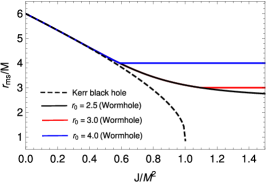
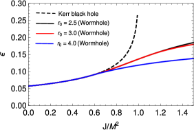
Figure 1: The Marginally stable circular orbits ($r_{ms}$) and the efficiency of an accretion disk ($\epsilon$), for different values of $J/M^{2}$ and $r_{0}$.

In Fig. 1, we have shown the dependence of the marginally stable circular orbits $r_{ms}$ and the efficiency $\epsilon$ of the accretion disk on of the angular momentum of the wormhole $J$ for different wormhole throat size $r_{0}$, along with the corresponding results for a Kerr black hole. From a physical point of view, the marginally stable circular orbits form the innermost stable circular orbits for the wormhole, beyond which the particle will fall into the throat and will be lost to the other universe. Note that, for a given angular momentum and throat size, $r_{ms}$ cannot be less than $r_{0}$. If all the roots of $\frac{d^{2}V_{eff}}{dr^{2}}=0$ are found to be smaller than $r_{0}$, then we take $r_{ms}=r_{0}$ as the throat acts as the position of the marginal stable orbits in that case. See (Paul, ) for more details. In Table 1, the numerical values of the position of marginally stable circular orbits $r_{ms}$ and the efficiency $\epsilon$ of the accretion disk, corresponding to various values of the angular momentum of the wormhole $J$ and throat size $r_{0}$, are tabulated, along with the corresponding results for a Kerr black hole.

Table 1: The Marginally stable circular orbits ($r_{ms}$) and the efficiency of the accretion disk ($\epsilon$), for different values of $J/M^{2}$ and $r_{0}$.

	$r_{ms}$ (in M)			Efficiency $\epsilon$
	Wormhole		Kerr Black	Wormhole		Kerr Black
$J/M^{2}$	$r_{0}=2.5M$	$r_{0}=4M$	hole	$r_{0}=2.5M$	$r_{0}=4M$	hole
0	6.0	6.0	6.0	0.05719	0.05719	0.05719
0.2	5.32761	5.32761	5.32944	0.06474	0.06474	0.064634
0.5	4.28536	4.28536	4.23300	0.08254	0.08254	0.08212
0.7	3.67576	4.0	3.39313	0.10112	0.09940	0.10361
0.9	3.25027	4.0	2.32088	0.12446	0.11299	0.15575
1.5	2.75805	4.0	—	0.18496	0.13821	—

To obtain the flux radiated, temperature and emission spectra of the disk, we consider the mass of the wormhole to be $M=15M_{\odot}$ (Imp, ) and the mass accretion rate to be $\dot{M}\approx 3\times 10^{-12}M$/year. Also, to obtain the results in the physical units, we restore $G$ and $c$ by replacing $M$ by $GM/c^{2}$ and $\dot{M}$ by $\dot{M}c^{2}$, where $G$ and $c$ are, respectively, Newton’s gravitational constant and speed of light in vacuum. The flux $F(r)$ and the temperature $T(r)$ of the disk for different values of the dimensionless spin $J/M^{2}$ and throat size $r_{0}$ are, respectively, plotted in Figs. 2 and 3, along with the corresponding results for a Kerr black hole. From the figures, we can note that the flux and the temperature sharply increase just near the throat $r_{0}$ and then decrease gradually. Similarly, the emission spectra of the disk for various values of the dimensionless spin $J/M^{2}$ is plotted in Fig. 4, along with the emission spectra of a Kerr black hole. Note that, when both the spin and throat size are small, the flux, the temperature and the emission spectra of the disk mimic those of a Kerr black hole. However, with increasing either the spin value or the throat size, the results for the wormhole start differing from those of a Kerr black hole. In Table 2, following (Imp, ), we have shown the critical frequency $\nu_{crit}$ at which the spectra of the disk have a maximum values $\nu L(\nu)$.

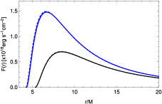
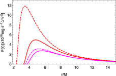
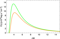
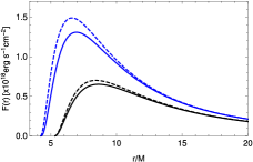
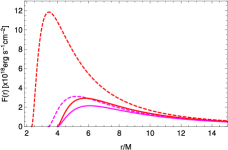
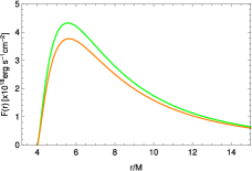
Figure 2: The energy flux radiated by the accretion disk around the wormhole (solid) for dimensionless spin values $J/M^{2}=0.2$ (black), $0.5$ (blue), $0.7$ (magenta), $0.9$ (red), $1.2$ (orange) and $1.5$ (green). The first and second row, respectively, corresponds to the throat size $r_{0}=2.5M$ and $4M$. For comparison, we also have shown the corresponding plots for a Kerr black hole (dashed) of same mass and spin. Some solid and dashed plots coincide with one another.

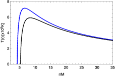
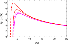
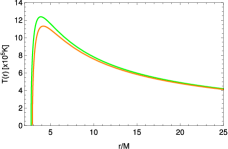
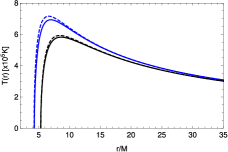
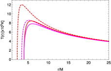
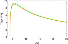
Figure 3: The temperature distribution of the accretion disk around the wormhole (solid) for dimensionless spin values $J/M^{2}=0.2$ (black), $0.5$ (blue), $0.7$ (magenta), $0.9$ (red), $1.2$ (orange) and $1.5$ (green). The first and second row, respectively, corresponds to the throat size $r_{0}=2.5M$ and $4M$. For comparison, we also have shown the corresponding plots for a Kerr black hole (dashed) of the same mass and spin. Some solid and dashed plots coincide with one another.

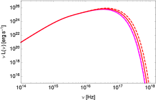
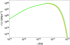
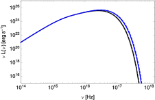
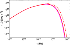
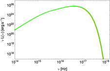
Figure 4: The emission spectra of the accretion disk around the wormhole (solid) for dimensionless spin values $J/M^{2}=0.2$ (black), $0.5$ (blue), $0.7$ (magenta), $0.9$ (red), $1.2$ (orange) and $1.5$ (green). The first and second row, respectively, corresponds to the throat size $r_{0}=2.5M$ and $4M$. For comparison, we also have shown the corresponding plots for a Kerr black hole (dashed) of the same mass and spin. Some solid and dashed plots coincide with one another.

Table 2: The critical frequency $\nu_{crit}$ at which the spectra has a maximum value $\nu_{crit}L_{max}(\nu_{crit})$ for different values of $J/M^{2}$ and $r_{0}$.

	$\nu_{crit}$($\times 10^{16}$ Hz)			$\nu_{crit}L_{max}(\nu_{crit})$ ($\times 10^{25}$erg $\text{s}^{-1}$)
	Wormhole		Kerr Black	Wormhole		Kerr Black
$J/M^{2}$	$r_{0}=2.5M$	$r_{0}=4M$	hole	$r_{0}=2.5M$	$r_{0}=4M$	hole
0.2	2.663	2.631	2.665	3.608	3.559	3.612
0.5	3.110	3.048	3.110	4.544	4.433	4.539
0.7	3.520	3.387	3.588	5.499	5.216	5.648
0.9	3.975	3.644	4.503	6.683	5.869	8.195
1.2	4.555	3.904	—	8.432	6.618	—
1.5	4.942	4.072	—	9.769	7.168	—

V Images of an accretion disk around the wormhole

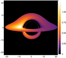
(a)  $J/M^{2}=0.2$ (Kerr black hole)

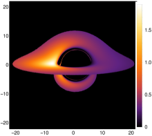
(b)  $J/M^{2}=0.5$ (Kerr black hole)

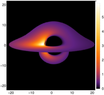
(c)  $J/M^{2}=0.9$ (Kerr black hole)

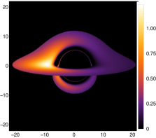
(d)  $J/M^{2}=0.2$, $r_{0}=2.5$ (Wormhole)

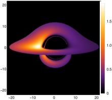
(e)  $J/M^{2}=0.5$, $r_{0}=2.5$ (Wormhole)

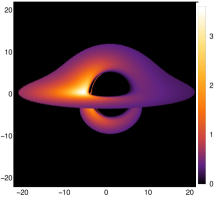
(f)  $J/M^{2}=0.9$, $r_{0}=2.5$ (Wormhole)

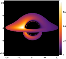
(g)  $J/M^{2}=0.5$, $r_{0}=3.0$ (Wormhole)

(h)  $J/M^{2}=0.5$, $r_{0}=4.0$ (Wormhole)

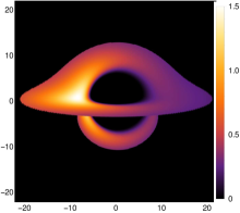
(i)  $J/M^{2}=0.5$, $r_{0}=5.0$ (Wormhole)

Figure 5: The images of an accretion disk in a Kerr black hole and rotating wormhole [(a)-(i)]. For wormhole, the disk is on the same side of the observer. The outer edge of the disk is at $r=20M$ , and the observer’s inclination angle is $\theta_{o}=80^{\circ}$. The observer is placed at the radial coordinate $r=10^{4}M$, which corresponds effectively to the asymptotic infinity. In order to get rid of the parameters $M$ and $\dot{M}$, we have normalized the fluxes by the maximum flux observed for the Schwarzschild black hole. Also, we have plotted square-root of the normalized flux for a better visualization. The color bars show the values the flux. All spatial coordinates are in units of $M$.

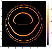
(a)  $J/M^{2}=0.2$, $r_{0}=2.5$ (Wormhole)

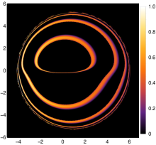
(b)  $J/M^{2}=0.5$, $r_{0}=2.5$ (Wormhole)

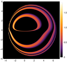
(c)  $J/M^{2}=0.9$, $r_{0}=2.5$ (Wormhole)

Figure 6: The images of an accretion disk in the rotating wormhole [(a)-(c)] when the disk is on the other side of the throat (i.e. the disk and the observer are on two opposite sides of the throat). The outer edge of the disk is at $r=20M$ , and the observer’s inclination angle is $\theta_{o}=80^{\circ}$. The observer is placed at the radial coordinate $r=10^{4}M$, which corresponds effectively to the asymptotic infinity. In order to get rid of the parameters $M$ and $\dot{M}$, we have normalized the fluxes by the maximum flux observed for the Schwarzschild black hole. Also, we have plotted square-root of the normalized flux for better looking. The color bars show the values of the flux. All spatial coordinates are in units of $M$.

We now consider how the image of an accretion disk around the wormhole looks like. In order to produce the intensity map of the image, we implement ray-tracing techniques discussed in (Paul, ; Shaikh_disk, ). We do not discuss the detailed procedure here as it can be found in (Paul, ; Shaikh_disk, ). Figure 5 shows how the image of an accretion disk looks like to an asymptotic observer when the disk and the observer are on the same side of the wormhole throat. For comparison, we also have shown the images for a Kerr black hole. Note that, when both the spin and the wormhole throat size are small, the images almost mimic those of the black hole (compare among Figs. 5(a),5(b), 5(d) and 5(e)). However, with increasing spin value or the throat size, the image starts differing both qualitatively and quantitatively from that of a Kerr black hole (compare the flux values and the inner thin rings in Figs. 5(c) and 5(f) and in Figs. 5(b), 5(h) and 5(i)). This indicates that, when the disk and the observer are on the same side, wormholes with larger spin or throat size can be distinguished from a Kerr black hole with the same spin through the observation of their disk images. Figure 6 shows the image of an accretion disk when the disk and the observer are on the two opposite sides of the wormhole throat. Note that, irrespective of the spin or the throat size, the images in this case are strikingly different from those of a Kerr black hole. In this case, a single intensity map of a disk image contains multiple images. This unique characteristic feature of the images can in principle be used to distinguish a wormhole from a black hole.

VI Concluding Remarks

In this paper, we have investigated thin accretion disk around a rotating traversable wormhole of Teo class Teo , of mass $M=15M_{\odot}$. We have studied the variation of the physical properties of our wormhole, with the spin parameter $J/M^{2}$ ranging from 0.2 to 1.5 and for two specific values of throat radius: $r_{0}=2.5M$ and $r_{0}=4M$; and hence compared those results with that of Kerr black hole. In classical theory of general relativity, traversable wormholes are supported by exotic matter in their throat, which is characterized by a stress energy tensor that violates the null energy condition. This unique feature may help to distinguish it and compare it with the Kerr black hole geometry. The expressions of the basic kinematic properties of the accretion disk, like angular velocity $\Omega$, specific energy $E(r)$, specific angular momentum $L(r)$ and effective potential term $V_{eff}$, are investigated analytically. The effect of changing the spin parameter $J/M^{2}$ on the marginally stable circular orbits $r_{ms}$ are studied graphically in figure 1.(a) corresponding to three values of throat radius: $r_{0}=2.5M$ (black),$3.0M$ (red) and $4.0M$ (blue); compared to the dashed curve representing the Kerr black hole. Note that the curves are almost overlapping for small values of $J/M^{2}$, but as $J/M^{2}$ increases beyond $0.5$ they separate out, though the value of $r_{ms}$ can never be less than the throat radius $r_{0}$, which explains the fact that each of the curve corresponding to different throat radius ends in a straight line with the constant value of $r_{ms}=r_{0}$ . The values of $r_{ms}$ are found to be decreasing with increase in $J/M^{2}$, but are more than the values obtained in case of Kerr black hole. The efficiency of accretion $\epsilon$ is plotted in figure 1(b). In general, for all the different values of throat radius $r_{0}$, efficiency increases with increase in $J/M^{2}$, but is found to be lesser than the Kerr black hole. For small value of $J/M^{2}$ the curves overlap but for $J/M^{2}>0.5$, we find that the efficiency for the wormhole decreases for increasing values of throat radius $r_{0}$. These features of marginally stable circular orbits $r_{ms}$ and efficiency $\epsilon$ can also be studied in details from table I, corresponding to the different $J/M^{2}$ values and for the two specific throat radius $r_{0}=2.5M$ and $4.0M$ . Note that the efficiency $\epsilon$ of accretion ranges between 5.7% to 18.5 % approximately.

Now to analyze the properties of the radiation emerging from the surface of the disk, we have plotted the energy flux of perfect black body radiation $F(r)$ [in $erg$ $sec^{-1}cm^{-2}$] and temperature distribution $T(r)$ [in $K$], in figures 2 and 3, respectively, for six different values of the dimensionless spin parameter $J/M^{2}$ ranging from 0.2 to 1.5 and for throat $r_{0}=2.5M$ (along first row) and $r_{0}=4M$ (along second row) and compared those with that of Kerr black hole (in dashed curves). The radiation flux is of the order of $10^{18}$ $ergsec^{-1}cm^{-2}$ while temperature is of order $10^{5}K$. In figure 4, the emission spectra $\nu L(\nu)$, [in $ergs^{-1}$] of the accretion disk around the wormhole is plotted corresponding to the different values of $J/M^{2}$ and $r_{0}$ as mentioned before. In table II, we have tabulated the value of frequency, called the critical frequency $\nu_{crit}$ where the emission spectra has a maximum value of luminosity of the disk $\nu_{crit}L_{max}(\nu_{crit})$, corresponding to the different values of the dimensionless spin parameter $J/M^{2}$ and the throat radius $r_{0}$; in order to understand in details the effect of these two parameters on the luminosity of the disk. From the table it is evident that, along each column corresponding to the two throat radius $r_{0}$ values, the critical frequency $\nu_{crit}$ increases with increase in spin parameter $J/M^{2}$; but along any row, corresponding to any particular value of $J/M^{2}$, the $\nu_{crit}$ value is slightly higher in case of lower value of throat radius $r_{0}$. Same trend is noted in case of the maximum luminosity values $\nu_{crit}L_{max}(\nu_{crit})$ column. It increases with the increase in $J/M^{2}$ along each column, when the $r_{0}$ values are kept constant; but along any particular row, corresponding to a constant value of $J/M^{2}$, the values are higher in case of the lower value of $r_{0}$. Also we can find that for lower values of both spin parameter $J/M^{2}$ and throat $r_{0}$, the critical frequency and maximum luminosity $\nu_{crit}L_{max}(\nu_{crit})$ are closer to the Kerr black hole case, but their difference gradually increases when the two parametric values increases.

In section V, we have tried to visualize the image of an accretion disk around the wormhole, by the intensity map of the image using ray-tracing techniques discussed in (Paul, ; Shaikh_disk, ). Figures 5.(d)-(i) shows how the image of an accretion disk looks like to an asymptotic observer when the disk and the observer are on the same side of the wormhole throat. Note that for smaller values of both the spin and the wormhole throat size , the images almost mimic those of the Kerr black hole shown in figures 5. (a)-(c), but when the spin parameter values or the throat radius is increased, the image starts differing qualitatively and quantitatively from that Kerr black hole. In figures 6.(a)-(c), the images of an accretion disk in the rotating wormhole are shown, as observed by an asymptotic observer , when the disk is on the other side of the throat (i.e.the disk and the observer are on two opposite sides of the throat). Note that, irrespective of the spin or the throat size, the images of the accretion disk when the observer is located at the opposite side of the throat, are strikingly different from those of a Kerr black hole; and a single intensity map of a disk image contains multiple images. This unique characteristic feature of the images can in principle be used to distinguish a wormhole from a black hole. Thus the detailed analysis of the physical and geometrical properties of these images, studied in this paper, could yield invaluable information on the nature of the accretion flows, in case of a rotating wormhole. Also the striking results from image analysis of its emission spectra could help to detect and distinguish wormhole geometries from other compact objects. We hope our work could be an interesting study and could motivate similar research in this field. For the Kerr black hole geometry, the horizons exist for $a<M$ case. For $a>M$, the horizons do not exist, and we have a Kerr naked singularity. While we hope that future observations might tell whether or not a Kerr naked singularity exists, on the theoretical front, there has been a lot of works on what could be observational aspects of a Kerr naked singularity if it exists in nature (new1, ; new2, ; new3, ; new4, ; new5, ). Moreover, in presence of other parameters (or hairs), a spacetime can represent a black hole even when $a>M$. For example, a tidally charged spacetime with $a>M$ can represent a black hole [ see (new6, ) for a work on its shadow in light of M87^∗ ]. Therefore, some black holes with parameters other than mass and spin or some horizonless object might have $a>M$, although their existence and otherwise should be confirmed through future observations.

Appendix

One can note that our Lorentzian wormhole has a throat at $r=r_{0}$. When $M=0$, we have the massless wormhole found by Ellis and Bronnikov (new7, ; new8, ). Also one can check that , $\partial_{\theta}b|_{r=r_{0}}=0$. Thus no event horizon or curvature singularity at the throat. For this choice of b the flare out condition $\partial_{r}b|_{r=r_{0}}<1$ and $b<r$ have been satisfied. The wormhole considered in eq. 27 was considered in reference [27] of our paper to study quasinormal ringing of a wormhole. It has been shown that, depending on the parameters, the wormhole may ring similarly or completely differently from that of a Kerr black hole. We took this metric to explore it in the context of accretion disk properties.

To check the traversability of this wormhole, let us find out the tidal acceleration at the throat. It shall be less than one earth gravity, i.e $\leq 9.8m/s^{2}$ for traversable. But, for simplicity, we consider the spin zero case below.

$$a^{\hat{j^{\prime}}} = -c^{2}R^{\hat{j}^{\prime}}_{\hat{0}^{\prime}\hat{k}^{\prime}\hat{0^{\prime}}}\xi^{\hat{k}}\textrm{[ see eq. 46 Morris and Thorne paper in reference [2] ]}$$

$${}^{\prime}a^{\prime} = -c^{2}R^{\hat{1}^{\prime}}_{\hat{0}^{\prime}\hat{1}^{\prime}\hat{0}^{\prime}}\xi^{\hat{1}}\textrm{( radial acceleration)}.$$

Now,

$$R^{\hat{1}^{\prime}}_{\hat{0}^{\prime}\hat{1}^{\prime}\hat{0}^{\prime}}=-\left(1-\frac{b}{r}\right)\bigg{[}-\phi^{\prime\prime}+\frac{b^{\prime}r-b}{2r(r-b)}\phi^{\prime}-{\phi}^{\prime 2}\bigg{]}.$$

Now,

$$e^{\phi} = \sqrt{1-\frac{2M}{r}}\Rightarrow\phi=\frac{1}{2}\log\bigg{(}1-\frac{2M}{r}\bigg{)},$$

$$\Rightarrow\phi^{\prime} = \frac{M/r^{2}}{1-\frac{2M}{r}}\Rightarrow\phi^{\prime\prime}=\frac{(1-\frac{2M}{r})(-\frac{2M}{r^{3}})-\frac{M}{r^{2}}\times\frac{2M}{r^{2}}}{(1-\frac{2M}{r})^{2}}$$

$$= \frac{-\frac{2M}{r^{3}}(1-\frac{2M}{r})}{(1-\frac{2M}{r})^{2}}.$$

$$b = \frac{r_{0}^{2}+2M(r-r_{0})}{r}=2M+\frac{r_{0}^{2}-2Mr_{0}}{r},$$

$$b^{\prime} = -\frac{r_{0}^{2}-2Mr_{0}}{r^{2}}.$$

$$R^{1}_{010} = -\left(1-\frac{b}{r}\right)\bigg{[}\frac{-\frac{2M}{r^{3}}(1-\frac{2M}{r})}{(1-\frac{2M}{r})^{2}}+\frac{\frac{M^{2}}{r^{4}}}{(1-\frac{2M}{r})^{2}}\bigg{]}-\frac{b^{\prime}r-b}{2r^{2}}\phi^{\prime}.$$

At throat $r=r_{0}$, first term is zero. Now

$$R^{\hat{1}^{\prime}}_{\hat{0}^{\prime}\hat{1}^{\prime}\hat{0}^{\prime}}|_{r=r_{0}} = -\frac{b^{\prime}r-b}{2r^{2}}\phi^{\prime}|_{r=r_{0}}$$

$$= \frac{1}{2r^{2}_{0}}\bigg{[}\frac{r_{0}^{2}-2Mr_{0}}{r_{0}}+\frac{r^{2}_{0}}{r_{0}}\bigg{]}\times\frac{\frac{M^{2}}{r^{2}_{0}}}{1-\frac{2M}{r_{0}}}$$

$$= \frac{1}{2r^{2}_{0}}[2r_{0}-2M]\times\frac{\frac{M^{2}}{r^{2}_{0}}}{1-\frac{2M}{r_{0}}}$$

$$= \frac{1}{r^{2}_{0}}\frac{\frac{M}{r_{0}}(1-\frac{M}{r_{0}})}{1-\frac{2M}{r_{0}}}.$$

Radial tidal acceleration of throat

$$\mid a^{\hat{i}^{\prime}}\mid|_{r=r_{0}}=c^{2}\xi^{\prime}\times\frac{1}{r^{2}_{0}}\frac{\frac{M}{r_{0}}(1-\frac{M}{r_{0}})}{1-\frac{2M}{r_{0}}}.$$

For a traveler of size $\xi^{\prime}=2$ meter and $r_{0}=2.5M=\frac{5}{2}M$,

$$\mid a^{\hat{i}^{\prime}}\mid|_{r=r_{0}}=2c^{2}\times\frac{4}{25M^{2}}\frac{\frac{2}{5}\times\frac{3}{5}}{\frac{1}{5}}=\frac{48c^{2}}{125M^{2}}.$$

Now $r_{0}=2.5M$ is in $G=c=1$ unit. In dimension full unit $M=\frac{GM}{c^{2}}$,

$$\mid a^{\hat{i}^{\prime}}\mid|_{r=r_{0}}=\frac{48}{125}\frac{c^{2}}{\frac{G^{2}M^{2}}{c^{4}}}=\frac{48}{125}\times\frac{c^{6}}{G^{2}M^{2}}.$$

If we take $M$ to be of that of $M87^{\star}$ as

$$M=6.5\times 10^{9}M_{0}=6.5\times 10^{9}\times 2\times 10^{30}kg=13\times 10^{39}kg,$$

then

$$\mid a^{\hat{i}^{\prime}}\mid|_{r=r_{0}}=\frac{48}{125}\times\frac{(3\times 10^{8})^{6}}{(6.67\times 10^{-11})^{2}(13\times 10^{39})^{2}}$$

$$\simeq~{}3.7\times 10^{-10}m/s^{2}$$

$$\Rightarrow\textrm{negligible because}~{}~{}a^{\prime}\sim\frac{1}{M^{2}}~{}~{}\textrm{and}~{}M~{}\textrm{is large.}$$

Similarly, $a^{2}$ and $a^{3}$ will be small $\Rightarrow$ Traversable.

References

- (1) M. Visser , Lorentzian Wormhole: from Einstein to Hawking , AIP Press (1995) .
- (2) M. Morris and K. Throne , American J. Phys. 56, 395 (1988 ).
- (3) Shakura NI, Sunyaev RA. Black holes in binary systems. Observational appearance. Astron Astrophys. 1973;24:337.
- (4) ID. Novikov , KS. Thorne, In: DeWitt C, DeWitt B, editors. Black Holes. New York: Gordon and Breach; 1973.
- (5) DN. Page , KS. Thorne Astrophys J. 1974;191:499.
- (6) KS. Thorne , Astrophys J. 1974;191:507.
- (7) J. P. Luminet, Astron. Astrophys. 75, 228(1979).
- (8) J. Gair, C. Li and I. Mandel, Phys. Rev. D 77, 024035 (2008).
- (9) S. Bhattacharyya , AV. Thampan , I. Bombaci , Astron Astrophys. 2001;372:925.
- (10) DF. Torres , Nucl Phys B. 2002;626:377.
- (11) YF. Yuan , R. Narayan , MJ. Rees , Astrophys J. 2004;606:1112.
- (12) FS. Guzman , Phys Rev D. 2006;73:021501.
- (13) Z. Kovacs , T. Harko , Phys Rev D. 2010;82:124047.
- (14) G. Gyulchev, P. Nedkova, T. Vetsov and S. Yazadjiev, Phys. Rev. D 100, 024055 (2019).
- (15) P. Bueno, P.A. Cano, F. Goelen, T. Hertog and B. Vercnocke, Phys. Rev. D 97, 024040 (2018).
- (16) R.Kh. Karimov, R.N. Izmailov, and K.K. Nandi,arXiv:1901.05762v4 [gr-qc] 4 Feb 2020.
- (17) T.Harko, Z. Kovacs , FSN. Lobo , Class Quant Grav. 2009;26:215006.
- (18) CSJ. Pun , Z. Kovacs , T. Harko , Phys Rev D. 2008;78:024043.
- (19) CSJ. Pun , Z. Kovacs , T. Harko, Phys Rev D. 2008;78:084015.
- (20) T. Harko, Z. Kovacs , FSN. Lobo , Class Quant Grav. 2010;27:105010.
- (21) T. Harko, Z. Kovacs , FSN. Lobo , Class Quant Grav. 2011;28:165001.
- (22) C. Liu1, C. Ding, J. Jing, arXiv:1910.13259v2 [gr-qc] 6 Nov 2019.
- (23) T. Harko, Z. Kovacs , FSN. Lobo , Phys Rev D. 2008;78:084005.
- (24) T. Harko, Z. Kovacs , FSN. Lobo , Phys Rev D. 2009;79:064001.
- (25) S. Paul, R. Shaikh, P. Banerjee, and T. Sarkar, JCAP 03, 055 (2020).
- (26) E. Teo, Phys. Rev. D 58, 024014 (1998).
- (27) R. A. Konoplya and A. Zhidenkob, JCAP 12, 043 (2016).
- (28) R.Kh. Karimov, R.N. Izmailov, and K.K. Nandi1, arXiv:1901.05762v4 [gr-qc] 4 Feb 2020.
- (29) R. Shaikh and P. S. Joshi, JCAP 10, 064 (2019).
- (30) Zdenek Stuchlík and Jan Schee, Class. Quantum Grav. 27 215017 (2010)
- (31) Zdenek Stuchlík and Jan Schee, Class. Quantum Grav. 29 025008 ( 2012)
- (32) Zdenek Stuchlík and Jan Schee , Class. Quantum Grav. 30 075012 (2013 )
- (33) Cosimo Bambi, Katherine Freese, Sunny Vagnozzi, and Luca Visinelli, Phys. Rev. D 100, 044057 (2019)
- (34) Chandrachur Chakraborty, Prashant Kocherlakota, Mandar Patil, Sudip Bhattacharyya, Pankaj S. Joshi, and Andrzej Królak, Phys. Rev. D 95, 084024 (2017)
- (35) Indrani Banerjee, Sumanta Chakraborty, and Soumitra SenGupta, Phys. Rev. D 101, 041301(R) (2020)
- (36) K. A. Bronnikov, Acta Phys. Pol. B4, 251 (1973)
- (37) H. G. Ellis, J. Math. Phys. 14, 104 (1973)