Inertial Particles in Superfluid Turbulence: Coflow and Counterflow

Abstract

We use pseudospectral direct numerical simulations (DNSs) to solve the three-dimensional (3D) Hall-Vinen-Bekharevich-Khalatnikov (HVBK) model of superfluid Helium. We then explore the statistical properties of inertial particles, in both coflow and counterflow superfluid turbulence (ST) in the 3D HVBK system; particle motion is governed by a generalization of the Maxey-Riley-Gatignol equations. We first characterize the anisotropy of counterflow ST by showing that there exist large vortical columns. The light particles show confined motion as they are attracted towards these columns and they form large clusters; by contrast, heavy particles are expelled from these vortical regions. We characterise the statistics of such inertial particles in 3D HVBK ST: (1) The mean angle $\Theta(\tau)$, between particle positions, separated by the time lag $\tau$, exhibits two different scaling regions in (a) dissipation and (b) inertial ranges, for different values of the parameters in our model; in particular, the value of $\Theta(\tau)$, at large $\tau$, depends on the magnitude of ${\bf U}_{ns}$. (2) The irreversibility of 3D HVBK turbulence is quantified by computing the statistics of energy increments for inertial particles. (3) The probability distribution function (PDF) of energy increments is of direct relevance to recent experimental studies of irreversibility in superfluid turbulence; we find, in agreement with these experiments, that, for counterflow ST, the skewness of this PDF is less pronounced than its counterparts for coflow ST or for classical-fluid turbulence.

I Introduction

Over the past few decades, there has been growing interest in studies of the statistical properties of particles advected by turbulent fluid flows, especially because of advances in experimental techniques and computational resources. Such particle advection is of central importance in geophysical Shaw2003 ; Grabowski2013 ; Falkovich2002 and astrophysical Armitage2010 flows, industrial process Eaton1994 ; Post2002 , nonequilibrium statistical mechanics Cardy2008 , and the visualization of turbulent flows in quantum fluids Donnelly1991 ; Paloetti2011 ; Skrbek2012 ; Berloff2014 ; Tsubota2017 ; BarenghiParker16 ; Bewley06 ; Bewley08 ; Poole2005 ; Mantia2013 ; Mantia2014 ; Zmeev2013 ; Guo14 ; Yang20 . However, investigations of particles in turbulent superfluids are in their infancy, when we compare them with their classical-fluid-turbulence counterparts. Some experimental groups Bewley06 ; Bewley08 ; Poole2005 ; Mantia2013 ; Mantia2014 ; Zmeev2013 ; Guo14 ; Yang20 ; Mantia2019 have used particles to visualize vortex lines in superfluid turbulence. In some cases the particles (e.g., frozen hydrogen or deuterium) are several orders of magnitude larger than the core size of a vortex. Some of these particles can be modeled as neutrally buoyant tracer particles in superfluid turbulence.

Superfluid turbulence is a multiscale problem for which we must use different levels of description, depending on the length scales that we consider Berloff2014 ; Tsubota2017 ; BarenghiParker16 : The Gross-Pitaevskii equation (GPE) Berloff2014 ; Krstulovic11 ; Shukla13 provides a natural description for a low-temperature, weakly-interacting Bose gas, at length scales comparable to the size of the superfluid vortex core, which has a healing length $\xi$. The vortex-filament model distinguishes between individual quantum vortices; but it does not account for the nature of the vortex core; it is valid on length scales greater than $\xi$, in the incompressible limit. The Hall-Vinen-Bekharevich-Khalatnikov (HVBK) two-fluid model does not resolve individual quantum vortices, but uses macroscopic, classical-vorticity fields (this assumes local polarization of quantum-vortex lines). At the level of kinetic theory, there is the model of Zaremba, Nikuni, and Griffin ZNG99 . Some groups have begun to investigate the interactions of classical particles with vortices in a GPE description of superfluid turbulence Winiecki00 ; Shukla16 ; Shukla18 ; Giuriato19 ; GPK19 ; GKN19 . These particles are active in the sense that they affect the superfluid flow while they are advected by this flow.

Within the HVBK framework, we can consider both coflow and counterflow Superfluid Turbulence (ST). In coflow ST, the two fluids move in the same direction, with the same mean velocities; in counterflow ST, superfluid and normal-fluid components move in opposite directions because of an imposed temperature gradient. The statistical properties of counterflow ST are different from those of classical-fluid turbulence sahoo and coflow ST Uns ; Polanco20 ; Lvov21 . In counterflow-ST experiments, there is a steady flow along a channel that is closed at one end and open at the other end; a heat flux $q$ is generated by passing a current through a resistor, at the closed end; the normal fluid, which carries this heat flux, with velocity ${\bf{U}}_{n}=q/\rho ST$, entropy per unit mass $S$, and at temperature $T$, moves away from the closed end; to maintain zero mass flux, $\rho_{s}{\bf U}_{s}+\rho_{n}{\bf U}_{n}=0$, so the superfluid flows in the opposite direction, towards the closed end, with velocity ${\bf{U}}_{s}=-(\rho_{n}/\rho_{s}){\bf{U}}_{n}$. Thus, there is a relative velocity ${\bf{U}}_{ns}={\bf{U}}_{n}-{\bf{U}}_{s}$ between the two fluids in such thermally driven counterflow STCarlo

$${\bf{U}}_{ns}=\frac{\rho}{\rho_{s}}{\bf{U}}_{n}$$ (1)

where $\rho_{n}$, $\rho_{s}$ are the densities of the normal-fluid and superfluid component respectively and $\rho=\rho_{n}+\rho_{s}$ is the total density. So long as the heat flux $q$ is small, this counterflow is laminar; but if $q$ increases beyond a critical value, this flow is turbulent.

We carry out a systematic study of inertial particles in 3D HVBK coflow ST and counterflow ST Donnelly1999 ; Barenghi1983 ; Hall1956 ; Khalatnikov1965 . This model has been studied, without particles, for superfluid ⁴He in both two dimensions (2D) and 3D Roche2009 ; Shukla2015 ; Biferale2019 ; Verma2019 ; moreover, a recent study Giorgio2020 has investigated the clustering of inertial particles in 3D HVBK turbulence. Below the critical temperature $T_{c}=2.17$K, superfluid ⁴He is thought of as comprising a viscous, normal-fluid component and an inviscid superfluid component. The density ratio of the normal-fluid component and the total fluid $(\rho_{n}/\rho)$ is equal to one at $T_{c}$; and $\rho_{n}/\rho$ decreases as we decrease the temperature $T$; at $T=0$ the normal-fluid component vanishes and ⁴He is completely in the superfluid form. For $0<T<T_{c}$, the normal-fluid component interacts with quantized vortices of the superfluid, via mutual friction Vinen1957 ; and this causes dissipation in the superfluid component. In this study, we consider inertial particles, whose size is smaller than the Kolmogorov dissipation length of the normal fluid; we assume that these particles are passive insofar as they do not affect the flow and their turbulence-induced accelerations are much larger than the acceleration because of gravity.

We use pseudospectral direct numerical simulations (DNSs) to solve a simplified version of the 3D HVBK model, with inertial particles, whose statistical properties we then study for different values of the mutual-friction coefficients, in this model, and for various values of the Stokes numbers ($St=\tau_{p}/\tau_{f}$, where, $\tau_{p}$ is the particle-response time and $\tau_{f}$ the Kolmogorov-dissipation time scale of the fluid). Inertial particles are different from Lagrangian tracer particles, which follow the fluid velocity; because of their inertia, particles cluster for $St\simeq 1$ Toschi2005 ; Biferale2005 ; Giorgio2020 . We summarize our principal results before we present the details of our work:

1. We characterize the anisotropy of counterflow ST by using spectra Lvov21 and the anisotropy tensor (see below); we then calculate particle statistics by employing the measures given below.

2. We define persistence times, based on the velocity-gradient tensors of the normal fluid and the superfluid, and show that the cumulative probability distribution functions (CPDFs) of these persistence times have exponential tails in different regions of the flow.

3. The mean angle $\Theta(\tau)$, between particle positions separated by the time lag $\tau$ (defined precisely below), has two different scaling regions (in dissipation and inertial ranges) for different values of the Stokes numbers and the mutual-friction coefficients.

4. The CPDFs of the curvature $\kappa$ and the modulus $\theta$ of the torsion of particle trajectories have power-law tails with universal exponents, which are independent of all the control parameters in our model.

5. We characterize the irreversibility of 3D HVBK turbulence, by using inertial particles, and quantify its dependence on the Stokes numbers.

The remainder of this paper is organised as follows. We describe the HVBK model and our DNSs in Sec. II. We present, in Sec. III, the details of our results.We discuss the implications of our results in the concluding Sec. Acknowledgments.

II Model and Numerical Simulations

We use the simplified form of the 3D HVBK equations Roche2009 . In addition to the kinematic viscosity $\nu_{\rm n}$ of the normal fluid, we include Vinen’s effective viscosity vinen2002quantum $\nu_{\rm s}$ in the superfluid component to mimic the dissipation because of (a) vortex reconnections and (b) interactions between superfluid vortices and the normal fluid 2007bottleneck ; The equations for this simplified, incompressible 3D HVBK model (we use the form suggested in Ref. Uns ) for fluctuations ${\bf u}_{n}$ and ${\bf u}_{s}$ with zero mean are:

$${\partial_{t}{\bf u}_{n}}+[({\bf u}_{n}+{\bf U}_{n})\cdot\nabla]{\bf u}_{n} = -\frac{1}{\rho_{n}}\nabla p_{n}+\nu_{n}\nabla^{2}{\bf u}_{n}$$

$$+ {\bf F}^{n}_{mf}+{\bf f}_{n},$$

$${\partial_{t}{\bf u}_{s}}+[({\bf u}_{s}+{\bf U}_{s})\cdot\nabla]{\bf u}_{s} = -\frac{1}{\rho_{s}}\nabla p_{s}+\nu_{s}\nabla^{2}{\bf u}_{s}$$ (2)

$$+ {\bf F}^{s}_{mf}+{\bf f}_{s}.$$

Here, ${\bf u}_{n}({\bf u}_{s})$, ${\bf U}_{n}({\bf U}_{s})$, $\rho_{n}(\rho_{s})$, $p_{n}(p_{s})$ and $\nu_{n}(\nu_{s})$ are the velocity, mean velocity, density, pressure, and kinematic viscosity of the normal fluid (superfluid), respectively; ${\bf U}_{n}$ and ${\bf U}_{s}$ vanish for coflow but not for counterflow. The mean relative velocity ${\bf U}_{ns}={\bf U}_{n}-{\bf U}_{s}$ is non-zero for counterflow and it cannot be eliminated by a Galilean transformation as discussed in Ref. Polanco20 . The mutual-friction terms ${\bf F}^{n}_{mf}$ and ${\bf F}^{s}_{mf}$, which lead to energy transfer between normal-fluid and superfluid components Morris2008 ; Wacks2011 , are

$${\bf F}^{s}_{mf} = -\frac{\rho_{n}}{\rho}{\bf f}_{mf};\;{\bf F}^{n}_{mf}=\frac{\rho_{s}}{\rho}{\bf f}_{mf};$$

$${\bf f}_{mf} = \frac{B}{2}\widehat{\omega}_{s}\times({\bf\omega}_{s}\times({\bf u}_{n}-{\bf u}_{s}))$$ (3)

$$+ \frac{B^{\prime}}{2}{\bf\omega}_{s}\times({\bf u}_{n}-{\bf u}_{s}),$$

where $\rho=\rho_{n}+\rho_{s}$ is the total density, ${\bf u}_{ns}={\bf u}_{n}-{\bf u}_{s}$ the slip velocity, $\omega_{s}=\nabla\times{\bf u}_{s}$ the superfluid vorticity, $B$ and $B^{\prime}$ the mutual-friction coefficients, and ${\bf f}_{n}$ and ${\bf f}_{s}$ the external forcing terms for the normal fluid and superfluid, respectively, and the caret denotes a unit vector. We consider incompressible flows for which we use the incompressibility conditions

$$\nabla\cdot{\bf u}_{n} = 0\,\,\,\,{\rm and}$$

$$\nabla\cdot{\bf u}_{s} = 0,$$ (4)

for the normal fluid and the superfluid, respectively. Given these incompressibility conditions, the pressures $p_{n}$ and $p_{s}$ can be eliminated from the equations; if these pressures are required, we can calculate them by using the Poisson equations that relate them to the velocity fields, but we do not need them in this study. We carry out a Fourier-pseudospectral DNS study of the 3D HVBK equations 2 and 4 by using the following:

• a cubical box of side $2\pi$, with periodic boundary conditions along each direction, $N^{3}$ collocation points, and the $2/3$ dealiasing rule Canuto1998 .

• in this pseudospectral method Krstulovic11 ; Orszag , the derivatives in Eq. 2 are evaluated in Fourier space where they are local, and products are evaluated in physical space; for Fast Fourier transforms (FFT) and their inverses we use the FFTW FFTW libraries:

• the constant-energy-injection scheme Lamorgese2005 ; Sahoo2011 is used to force the Fourier modes, which lie in the first two shells in Fourier space, for both the normal fluid and the superfluid;

• the second-order Adams-Bashforth scheme for time marching Sahoo2011 .

• In our direct numerical simulations (DNSs), we use smooth initial conditions; furthermore, the flow is incompressible, so there are no shocks. Of course, we do use $2/3$ dealiasing, as we have mentioned in our paper; we have checked explicitly, by using two resolutions, namely, $N^{3}=256^{3}$ and $N^{3}=512^{3}$ that the statistical properties we consider are not affected significantly by this change of resolution.

The parameters for our DNSs are given in Table 1; here, $Re_{\lambda}^{n}(Re_{\lambda}^{s})$, $\tau_{eddy}^{n}(\tau_{eddy}^{s})$, $\eta_{n}(\eta_{s})$, $\tau^{n}_{\eta}(\tau^{s}_{\eta})$, and $T$ are the Taylor-microscale Reynolds number, eddy-turn-over time, Kolmogorov dissipation length and time scales for the normal fluid (superfluid), and temperature (in Kelvin), respectively. We use the temperature-dependent values of $\rho_{n},\rho_{s},B$, and $B^{\prime}$ from the experiments of Ref. Donnelly1998 . The values of the viscosities are taken from Ref. viscosity . We use $\nu_{n}/\nu_{s}\leq 10$; it is difficult to go beyond this ratio with the resolution of our DNS. [This is similar to the problem faced by DNSs of magnetohydrodynamics (MHD) turbulence when the magnetic Prandtl number (the ratio of the fluid kine- matic viscosity and magnetic diffusivity ) is very different from unity Sahoo2011 .]

To study the advection of inertial particles in this HVBK model, we consider that (a) the radius of the particles $a\ll\eta_{n}$, where $\eta_{n}$ is the Kolmogorov dissipation length scales for normal fluid, (b) particles do not interact with each other, (c) particles do not affect the fluid flows, and (d) turbulence-induced particle accelerations are much greater than the acceleration because of gravity. The particle’s radius $\simeq 1\to 5\times 10^{-3}cm$; and the Kolmogorov length scale for normal fluid at $T=1.65K$ is $\simeq 1\times 10^{-2}cm$. Under these conditions, the evolution equations for the particles, discussed in Refs. Gatignol1983 ; Maxey1983 ; Bec2006 for a classical fluid, can be generalized, in the HVBK model Poole2005 , to:

$$\frac{d{\bf v}(t)}{dt} = \frac{{\bf u}_{n}({\bf X},t)-{\bf v}(t)}{\tau_{p}}+\beta\left(\frac{\rho_{n}}{\rho}\frac{D{\bf u}_{n}}{Dt}+\frac{\rho_{s}}{\rho}\frac{D{\bf u}_{s}}{Dt}\right)$$

$$\frac{d{\bf X}(t)}{dt} = {\bf v}(t);$$ (5)

here, ${\bf v}(t)$ and ${\bf X}(t)$ are, respectively, the velocity and position of the particle at time $t$; and ${\bf u}_{n}({\bf X},t)$ and ${\bf u}_{s}({\bf X},t)$ are the Eulerian normal-fluid and superfluid velocities at position $\bf X$ and time $t$; $D/Dt$ is the material derivative; the term with the coefficient

$$\beta\equiv 3\rho/(2\rho_{p}+\rho)$$ (6)

accounts for added-mass effects ($\rho_{p}$ is the particle’s density); the particle-response time for the normal fluid is:

$$\tau_{p}=\frac{a^{2}\rho}{3\beta\rho_{n}\nu_{n}};$$ (7)

To study the statistical properties of such particles, we solve Eq. 5 for (a) $N_{p}=100000$ particles, by using the first-order Euler scheme for time marching and tri-linear interpolation, to calculate the particles’ velocities at off-grid points, and (b) for different Stokes numbers

$${\rm{St_{n}}}=\frac{\tau_{p}}{\tau_{n}}$$ (8)

with $\tau_{n}=(\nu_{n}/\epsilon_{n})^{\frac{1}{2}}$ the Kolmogorov time scale for the normal fluid and $\epsilon_{n}$ is the rate of kinetic energy dissipation for the normal fluid; the higher these Stokes numbers, the higher the particle inertia.

$Run$	$N$	$T$	$\rho_{n}/\rho$	$\widetilde{U}_{ns}$	$B$	$B^{\prime}$	$\nu_{n}/10^{4}$	$\nu_{s}/10^{4}$	$dt/10^{4}$	$f_{n}$	$f_{s}$	$Re_{\lambda}^{n}$	$Re_{\lambda}^{s}$	$\tau_{eddy}^{n}$	$\tau_{eddy}^{s}$	$k_{max}\eta_{n}$	$k_{max}\eta_{s}$	$\tau^{n}_{\eta}$	$\tau^{s}_{\eta}$
$\bf R1$	$256$	$1.65$	$0.193$	0.00	$1.14$	$0.15$	$11.3$	$2.3$	$10$	$0.02$	$0.02$	$34$	$124$	$1.43$	$1.34$	$1.26$	$0.46$	$0.19$	$0.13$
$\bf R2$	$256$	$2.10$	$0.741$	0.00	$1.30$	$-0.07$	$1.67$	$10$	$10$	$0.02$	$0.02$	$153$	$40$	$1.30$	$1.41$	$0.36$	$1.14$	$0.11$	$0.18$
$\bf R3$	$512$	$1.65$	$0.193$	0.00	$1.14$	$0.15$	$11.3$	$2.3$	$8$	$0.02$	$0.02$	$35$	$211$	$1.24$	$1.14$	$2.04$	$0.49$	$0.15$	$0.09$
$\bf R4$	$256$	$1.65$	$0.193$	$11.32$	$1.14$	$0.15$	$11.3$	$2.3$	$10$	$0.02$	$0.02$	$287$	$758$	$1.60$	$1.45$	$2.45$	$0.68$	$0.58$	$0.29$
$\bf R5$				$20.31$								$237$	$561$	$1.90$	$1.65$	$2.46$	$0.71$	$0.74$	$0.31$
$\bf R6$	$256$	$2.10$	$0.741$	$8.94$	$1.30$	$-0.07$	$1.67$	$10$	$10$	$0.02$	$0.02$	$374$	$177$	$1.82$	$2.10$	$0.50$	$2.14$	$0.21$	$0.63$
$\bf R7$	$512$	$1.65$	$0.193$	$12.90$	$1.14$	$0.15$	$11.3$	$2.3$	$8$	$0.02$	$0.02$	$58$	$244$	$4.32$	$2.51$	$6.22$	$1.77$	$1.17$	$0.47$
$\bf R8$	$512$	$2.10$	$0.741$	$8.54$	$1.30$	$-0.07$	$1.7$	$10.0$	$8$	$0.02$	$0.02$	$190$	$62$	$2.17$	$4.12$	$1.13$	$5.40$	$0.26$	$1.00$

Table 1: Parameters for our DNS runs. Coflow ST: $\bf R1$ - $\bf R3$; and counterflow ST: $\bf R4$ - $\bf R8$. $N^{3}$ is the total no of collocation points; $\rho_{n}/\rho$ is the normal-fluid fraction; the non-dimensionalized counterflow velocity $\widetilde{U}_{ns}=|{\bf U}_{ns}|/u_{T}^{n}$, where $u_{T}^{n}=\sqrt{\langle|{\bf u}_{n}|^{2}\rangle}$ and the angular brackets denote the average over the turbulent, but statistically steady, state of the 3D HVBK system; $B$ and $B^{\prime}$ are the coefficients of mutual friction; $\nu_{n}(\nu_{s})$, $Re_{\lambda}^{n}(Re_{\lambda}^{s})$, $\tau_{eddy}^{n}(\tau_{eddy}^{s})$, $\eta_{n}(\eta_{s})$, $\tau^{n}_{\eta}(\tau^{s}_{\eta})$, and $T$ are the kinematic viscosity, Taylor-microscale Reynolds number, eddy-turn-over time, Kolmogorov dissipation length and time scales for the normal fluid (superfluid), and temperature (in Kelvin), respectively; the time step is $dt$; $k_{max}$ is the largest wave number (after dealiasing); and $f_{n}$ ($f_{s}$) provide constant energy injection into the first two shells in Fourier space for the normal fluid (superfluid); we force both the fluids.

III Results

We study the statistics of inertial particles for different values of ${\rm St}_{\rm n}$ and $\beta$ in the 3D HVBK model for our different DNS runs. Before we discuss these statistics of inertial particles we present, in Fig. 1, isosurface plots of the magnitude of the normal-fluid vorticity $|\omega_{n}|$ at $T=1.65$K: Figures 1(a) and (b)-(d) show, respectively, such isosurface plots for coflow and counterflow ST; in the latter case, the counterflow velocity points along $\widehat{\bf U}_{ns}=\hat{e}_{k}$, where $\hat{e}_{k}$ is the unit vector along the $z$ direction. We present isosurfaces for $\rm St_{n}=1.0$ and $\beta=1.25\,(\rho_{p}/\rho=0.7)$ and $\beta=0.1\,(\rho_{p}/\rho=14.5)$. For coflow, the spatial organization of isosurfaces appears to be isotropic at $T=1.65K$ and particles form clusters [Fig. 1(a)] as in classical fluid turbulence. In contrast, counterflow ST exhibits large-scale vortex columns (Fig.1(b)), in which heavy particles ($\beta=0.1$) form large clusters [Fig. 1(c)] that are repelled from the regions with large vortical structures; however, light particles ($\beta=1.25$) are attracted towards these structures [Fig. 1(d)]. In Fig.S10 of the Supplementary MaterialV , we show isosurface plots of $|\omega_{n}|$ for counterflow ST at $T=2.10K$; the distribution of particles is similar to that at $T=1.65K$.

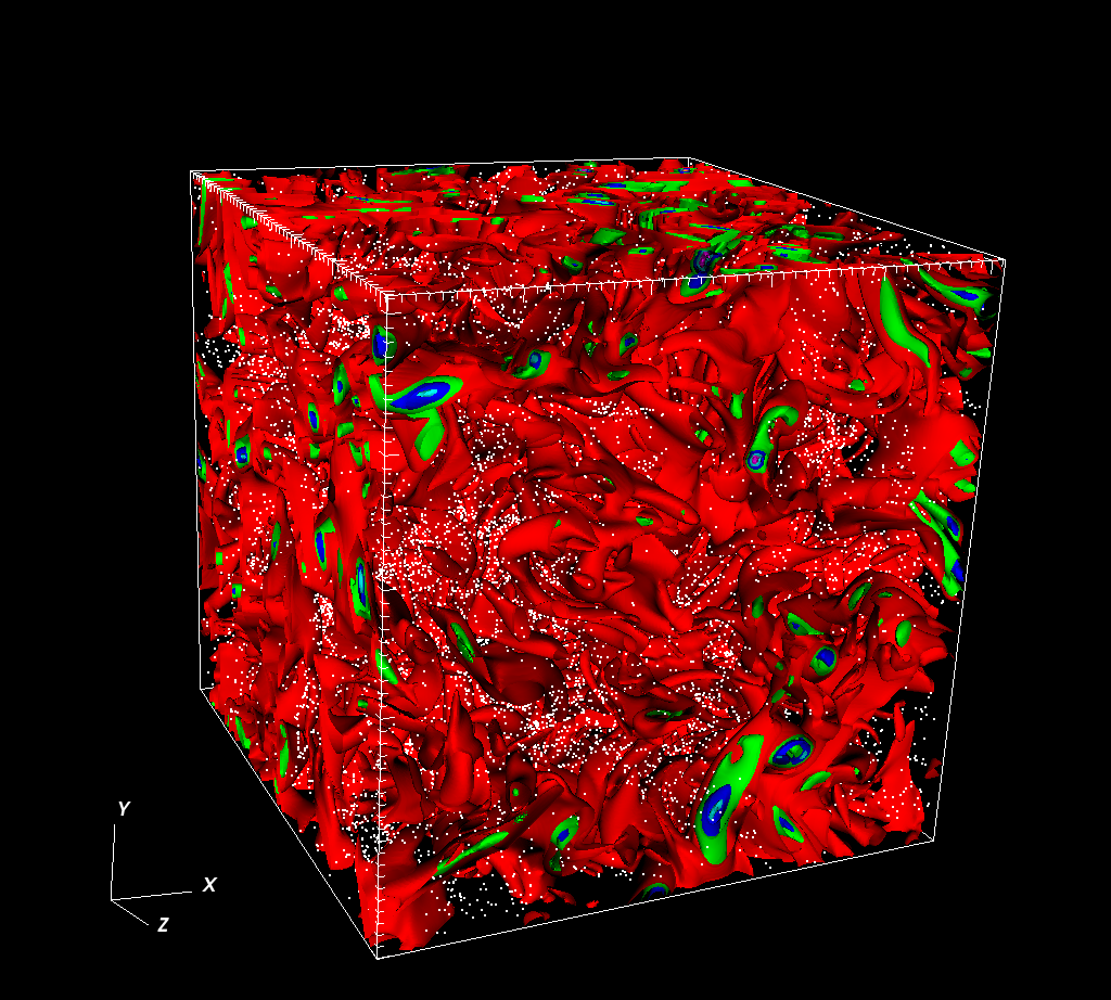
Figure 1: Isosurface plots of the magnitude of the normal-fluid vorticity $|\omega_{n}|$ with particles as white points, at $T=1.65$K. (a) coflow ST(R1) and (b)-(d) counterflow ST (R5); (c) a 2D view of (b) for heavy particles ($\beta=0.1$); and (d) the same plot as in (c) but for light particles ($\beta=1.25$). The counterflow velocity is along the $z$-direction, which points out of the page in (c).

We also characterize the anisotropy of counterflow ST by using the anisotropy tensor $a_{ij}$ and energy spectra. The anisotropy tensor has the components

$$a_{ij}=\frac{\overline{u_{i}u_{j}}}{\overline{u_{i}u_{i}}}-\frac{1}{3}\delta_{ij},$$ (9)

where $u_{i}$ and $u_{j}$ are the Cartesian components of the fluctuating velocity for the normal fluid, we use the Einstein summation convention for repeated indices, and the overbar denotes the volume average. We calculate different off-diagonal components of $a_{ij}$ and find, e.g., that $a_{ij}\simeq 10^{-3}$ for coflow ST at $T=1.65K$; by contrast, for counterflow ST, $a_{ij}\simeq 2\times 10^{-1}$. This shows clearly the degree of anisotropy in the counterflow ST in our DNS. Furthermore, we examine the anisotropy of counterflow ST by using the following energy spectra Lvov21 :

$$E^{l}_{k_{\parallel}} = \frac{1}{2}\sum_{k_{\parallel}-\frac{1}{2}<k^{\prime}<k_{\parallel}+\frac{1}{2}}\tilde{{\bf u}}^{l}_{\parallel}({\bf k}^{\prime})\cdot\tilde{{\bf u}}^{l}_{\parallel}(-{\bf k}^{\prime});$$

$$E^{l}_{k_{\perp}} = \frac{1}{2}\sum_{k_{\perp}-\frac{1}{2}<k^{\prime}<k_{\perp}+\frac{1}{2}}\tilde{{\bf u}}^{l}_{\perp}({\bf k}^{\prime})\cdot\tilde{{\bf u}}^{l}_{\perp}(-{\bf k}^{\prime});$$ (10)

here, $l$ can be $n$ or $s$; we denote by $\tilde{{\bf u}}^{l}_{\parallel}$ and $\tilde{{\bf u}}^{l}_{\perp}$ the spatial Fourier transforms of the velocities in the directions ${\bf k}_{\parallel}$ and ${\bf k}_{\perp}$, respectively, where ${\bf k}_{\parallel}=({\bf k}\cdot{\bf\widehat{U}}_{ns}){\bf\widehat{U}}_{ns}$ and, perpendicular to it, ${\bf k}_{\perp}={\bf k}-{\bf k}_{\parallel}$; and $k^{\prime},\,k_{\parallel}$, and $k_{\perp}$ are, respectively, the magnitudes of ${\bf k}^{\prime}$, ${\bf k}_{\parallel}$, and ${\bf k}_{\perp}$.

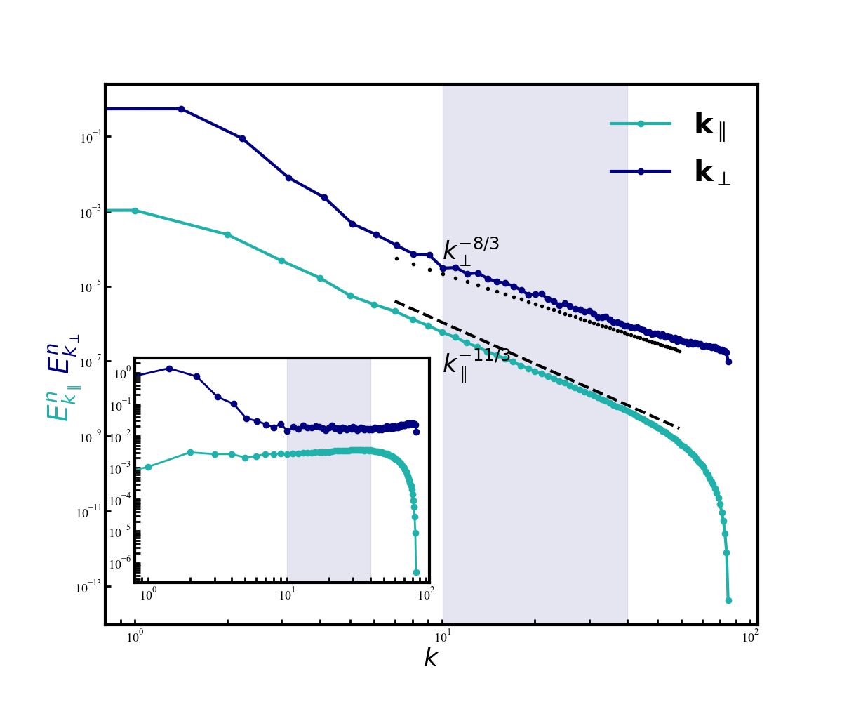
Figure 2: Log-log plots of the energy spectra (Eq. 10) $E^{n}_{k_{\perp}}$ (dark blue) and $E^{n}_{k_{\parallel}}$ (cyan) for the normal fluid component of counterflow ST with $T=1.65K$ and $\widehat{\bf U}_{ns}=\widehat{e_{k}}$ (run $\bf R5$). The blue shaded region shows the inertial range of scales. In the inset, we plot the compensated spectra $E^{n}_{k_{\perp}}*k_{\perp}^{8/3}$ (dark blue) and $E^{n}_{k_{\parallel}}*k_{\parallel}^{11/3}$ (cyan).

We plot, in Fig.2, the compensated energy spectra $E^{n}_{k_{\perp}}*k_{\perp}^{8/3}$ (dark blue) and $E^{n}_{k_{\parallel}}*k_{\parallel}^{11/3}$ (cyan) for the normal-fluid component of counterflow ST at $T=1.65K$ for ${\bf\widehat{U}}_{ns}=\widehat{e_{k}}$ (run $\bf R5$). Note that $E^{n}_{k_{\parallel}}$ is strongly suppressed relative to $E^{n}_{k_{\perp}}$; furthermore, these spectra show two distinct (blue-shaded region) power-law forms that are consistent with $E^{n}_{k_{\perp}}\sim k_{\perp}^{-8/3}$ and $E^{n}_{k_{\parallel}}\sim k_{\parallel}^{-11/3}$ . These spectra are in agreement with the recent results of Ref. Lvov21 .

This anisotropy of counterflow ST affects the trajectories of inertial particles, which are advected by such turbulence. We can visualise this qualitatively by including the positions of, say, $10000$ particles (shown via small white spheres) along with the isosurfaces, in Fig.1, of the magnitude of the normal-fluid vorticity $|\omega_{n}|$. Clearly, in the case of counterflow ST at $T=1.65$K ((c) of Fig. 1), particles form large clusters around large vortical structures and move principally along the direction $\widehat{\bf U}_{ns}$ of the counterflow velocity.

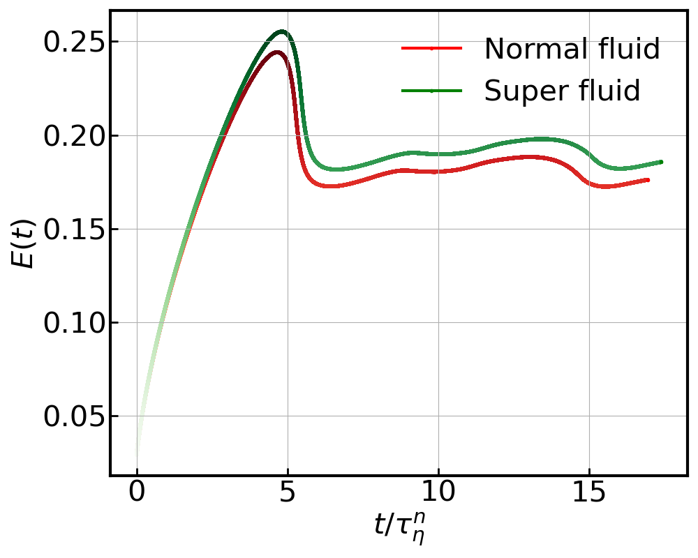
Figure 9: Plot of the volume-averaged energy, $E(t)=\sum_{k_{\parallel}}E_{k_{\parallel}}+\sum_{k_{\perp}}E_{k_{\perp}}$, of the turbulent flow for normal fluid and super-fluid components showing the statistically steady state at long times. Here $E_{k_{\parallel}}$ and $E_{k_{\perp}}$ are defined in Eqs.10 and $\tau_{\eta}^{n}$ is the dissipation time scale for the normal fluid.

In Subsection III.1 we characterize the flow in the Eulerian frame by using joint PDFs (JPDFs) of the $Q$ and $R$ invariants of the velocity-gradient tensor. In Subsection III.2 we obtain the angle $\Theta$ that quantifies the statistics of inertial-particle displacement increments. Subsection III.3 is devoted to a characteriation of the statistical properties of the geometry of particle trajectories. In Subsection III.4, we characterize the irreversibility of 3D HVBK turbulence. In all these Subsections we compare and contrast our results for coflow ST and counterflow ST; we also examine the dependence of some of the results on the non-dimensionalized counterflow velocity $\widetilde{U}_{ns}=|{\bf U}_{ns}|/u_{T}^{n}$, where $u_{T}^{n}=\sqrt{\langle|{\bf u}_{n}|^{2}\rangle}$ and the angular brackets denote the average over the turbulent, but statistically steady, state of the 3D HVBK system. Figure 9 in the Appendix shows the time series of the volume-averaged energy, $E(t)=\sum_{k_{\parallel}}E_{k_{\parallel}}+\sum_{k_{\perp}}E_{k_{\perp}}$, in the statistically steady state for run R1; here $E_{k_{\parallel}}$ and $E_{k_{\perp}}$ are defined in Eqs.10.

III.1 Joint probability distribution of Q-R invariants

We begin by calculating the invariants $P_{\rm a}$, $Q_{\rm a}$, and $R_{\rm a}$ of the velocity-gradient tensor $\mathcal{A}_{{\rm a}{ij}}={\partial_{j}u_{{\rm a}i}}$:

$$P_{\rm a} = -{\rm Tr}(\mathcal{A}_{\rm a});$$

$$Q_{\rm a} = -\frac{1}{2}{\rm Tr}(\mathcal{A}_{\rm a}^{2});$$

$$R_{\rm a} = -\frac{1}{3}{\rm Tr}(\mathcal{A}_{\rm a}^{3});$$ (11)

where the subscript a stands for $n$ or $s$, and $i,j=1,2,3$. For incompressible flows, $P_{\rm a}=0$. The discriminant for the characteristic equation of $\mathcal{A}_{\rm a}$ is

$$\Delta_{\rm a}=\frac{27}{4}R_{\rm a}^{2}+Q_{\rm a}^{3}.$$ (12)

We use these invariants and $\Delta_{\rm a}$, in the $Q_{\rm a}-R_{\rm a}$ plane, to characterize the following four types of flows regions (for this well-established method see, e.g., Ref. Akshaypersistence and references therein):

• Region A: vortical flow with stretching, for $\Delta_{\rm a}>0$ and $R_{\rm a}<0$;

• Region B: vortical flow with compression, for $\Delta_{\rm a}>0$ and $R_{\rm a}>0$;

• Region C: flow with biaxial strain, for $\Delta_{\rm a}<0$ and $R_{\rm a}<0$;

• and Region D: flow with axial strain, for $\Delta_{\rm a}<0$ and $R_{\rm a}>0$.

Joint PDFs (JPDFs) of $Q_{a}$ and $R_{a}$ are often used to characterize turbulent flows in classical-fluid turbulence Akshaypersistence , where they have a characteristic tear-drop shape, i.e., in strain-dominated regions ($Q<0$), $R>0$ is more probable than $R<0$, whereas the opposite holds in vortical regions ($Q>0$). In Fig. 3 we present filled contour plots of four representative JPDFs for coflow ST (Fig. 3 (a) and (b)) and counterflow ST (Fig. 3 (c) and (d)) at $T=1.65K$; these are in the Eulerian frame. The four flow regions, (A)-(D), are shown in Fig.3(a). We note that the JPDFs for coflow ST have a tear-drop shape, as in classical-fluid turbulence; but those for counterflow ST show some deviations from this shape, which means that, in the strain-dominated region ($Q<0$), both $R<0$ and $R>0$ are almost equally probable (and likewise for the vortical region ($Q>0$)). Some groups velocity_gradient have found, for various experimental turbulent flows, that the shape of the $Q-R$ JPDF depends on the flow and that deviations from a tear-drop shape may arise if we have vortex-sheet-like structures rather than vortex-tube-like structures; these depend on the sign of the second eigen value of strain-rate tensor. We will discuss this in detail, in the context of counterflow ST, elsewhere. In this paper, we focus principally on our particle-based studies.

In each one of these flow regions, (A)-(D), we calculate the PDFs of persistence times $t^{per}_{n}$ and $t^{per}_{s}$ for the normal-fluid ($n$) and superfluid ($s$) components, respectively. These are the times spent by a particle, in a given region, before it moves to another region. [For classical-fluid turbulence, see Ref. Akshaypersistence ]. We calculate persistence-time PDFs in the Eulerian frame, by measurements of $Q_{\rm a},R_{\rm a}$ and $\Delta_{\rm a}$, at a fixed point in space, as a function of time $t$. We get similar PDFs for tracers or inertial particles by following the trajectory of each such particle and obtaining $Q_{\rm a},R_{\rm a}$ and $\Delta_{\rm a}$ along its trajectory.

In Fig. 4 we present semilog plots of the persistence-time CPDFs at two temperatures ($T=1.65$K and $2.10$K), in the Eulerian frame, for the normal fluid and for coflow ST in Fig. 4(a) and for counterflow ST in Fig.4(b). We give similar plots for the superfluid component, in Fig.S11, in the Supplementary MaterialV. From the semilog plots in Figs. 4 and S11, we observe that, for both coflow and counterflow ST, persistence-time CPDFs (and PDFs) have exponentially decaying tails in all the regions A-D and in both the normal fluid and the superfluid.

Figure 3: Filled contour plots of four representative JPDFs for coflow ST [(a) and (b) from run R3] and counterflow ST [(c) and (d) from run R7]; we give JPDFs of $Q_{\rm n}$ and $R_{\rm n}$ in the first and third column and of $Q_{\rm s}$ and $R_{\rm s}$ in the second and fourth column; these are in the Eulerian frame. $\Lambda_{n}=\frac{u_{\eta_{n}}}{\eta_{n}}$ and $\Lambda_{s}=\frac{u_{\eta_{s}}}{\eta_{s}}$.

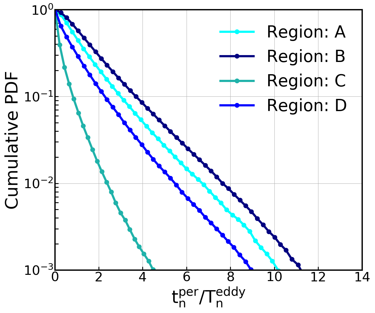
Figure 4: Semilog plots of the CPDFs of the persistence times, $t^{per}_{n}$, at $T=1.65K$ in the Eulerian frame for the normal-fluid ($n$) component; for coflow ST (run R3) in (a) and for counterflow ST (run R7) in (b).

III.2 Inertial-particle Displacement Increments

In the context of classical-fluid turbulence, it has been noted in Ref. Bos2015 that the study of the changes in direction of Lagrangian tracers reveals two power-law ranges. We carry out the analog of this analysis for inertial particles advected by 3D HVBK coflow and counterflow ST; our study highlights the effect of $\widetilde{U}_{ns}$ on the change in direction of these particles. From our DNSs, we obtain the angle $\Theta(\tau)$ between subsequent inertial-particle-displacement increments Bos2015 as a function of the time lag $\tau$ as follows:

$$\delta{\bf X(x}_{0},t,\tau)={\bf X(x}_{0},t)-{\bf X(x}_{0},t-\tau),$$ (13)

where ${\bf X(x}_{0},t)$ is the position of the particle at time $t$, ${\bf x}_{0}$ is the reference position for the particle at time $t_{0}$. The angle $\Theta(t,\tau)$ is given by

$$\cos(\Theta(t,\tau))=\frac{\delta{\bf X(x}_{0},t,\tau)\cdot{\delta\bf X(x}_{0},t+\tau,\tau)}{{\left|\delta{\bf X(x}_{0},t,\tau)\right|}{\left|\delta{\bf X(x}_{0},t+\tau,\tau)\right|}},$$ (14)

whose average value, over the time $t$ and the number of particles $N_{p}$, is

$$\Theta(\tau)=\langle{\left|\Theta(t,\tau)\right|}\rangle_{t,N_{P}}.$$ (15)

For coflow ST at $T=1.65$K [Fig. 5(a)], we present log-log plot of $\Theta(\tau)$ versus $\tau$ for different values of $\rm{St_{n}}$ and $\beta=1.25(\rho_{p}/\rho o=0.7)$. These plots show two power-law scaling regions separated by a crossover regime around $\tau_{\eta}^{n}$, the Kolmogorov time scale: in the dissipation range (cyan-shaded regions) $\Theta(\tau)\sim\tau^{\alpha}$; in the inertial range (green-shaded regions) $\Theta(\tau)\sim\tau^{\zeta}$; our data are consistent with the exponents $\alpha\simeq 1$ and $\zeta\simeq 1/2$. Similar scaling regimes have been obtained for Lagrangian tracers in classical-fluid turbulence Bos2015 except at large Stokes number in which case particles become ballistic and do not show the inertial range. This shows that coflow ST at $T=1.65$K or higher temperatures behaves like classical fluid turbulence because the normal-fluid and superfluid components are strongly coupled by the mutual friction.

For counterflow ST at $T=1.65$K (Fig. 5(b)), the scaling region in the dissipation range ($\tau<\tau_{\eta}^{n}$) yields $\alpha\simeq 1$, as in coflow ST. Beyond $\tau_{\eta}^{n}$, because of the mean counterflow speed ($\tilde{U}_{ns}=20.31$), particles form large clusters (Fig.1(b)-(d)). For light particles (Fig.1(d)), these large clusters are attracted towards the vortex columns and are substantially confined. This confinement reduces asymptotic value of $\Theta$ at large $\tau$ (as compared to its counterpart in coflow ST). In particular, particles with large $\rm St_{n}$ (cyan curve in Fig.5(b)) are strongly affected by this confinement because they follow the normal-fluid component, which has large mean velocity ${\bf U}_{n}$ as compared to that of the superfluid component ${\bf U}_{s}$ [cf. Ref. confinement for a related effect in classical-fluid turbulence]. At a higher temperature, say $T=2.10K$, the superfluid fraction is very small and the behavior of $\Theta$ is similar to that in classical fluid turbulence [Fig.5(c)] with the scaling exponents $\alpha\simeq 1$ and $\zeta\simeq 1/2$; of course, at large values of $\tau$, $\Theta$ is reduced, because of the mean counterflow velocity, as it is for $T=1.65K$.

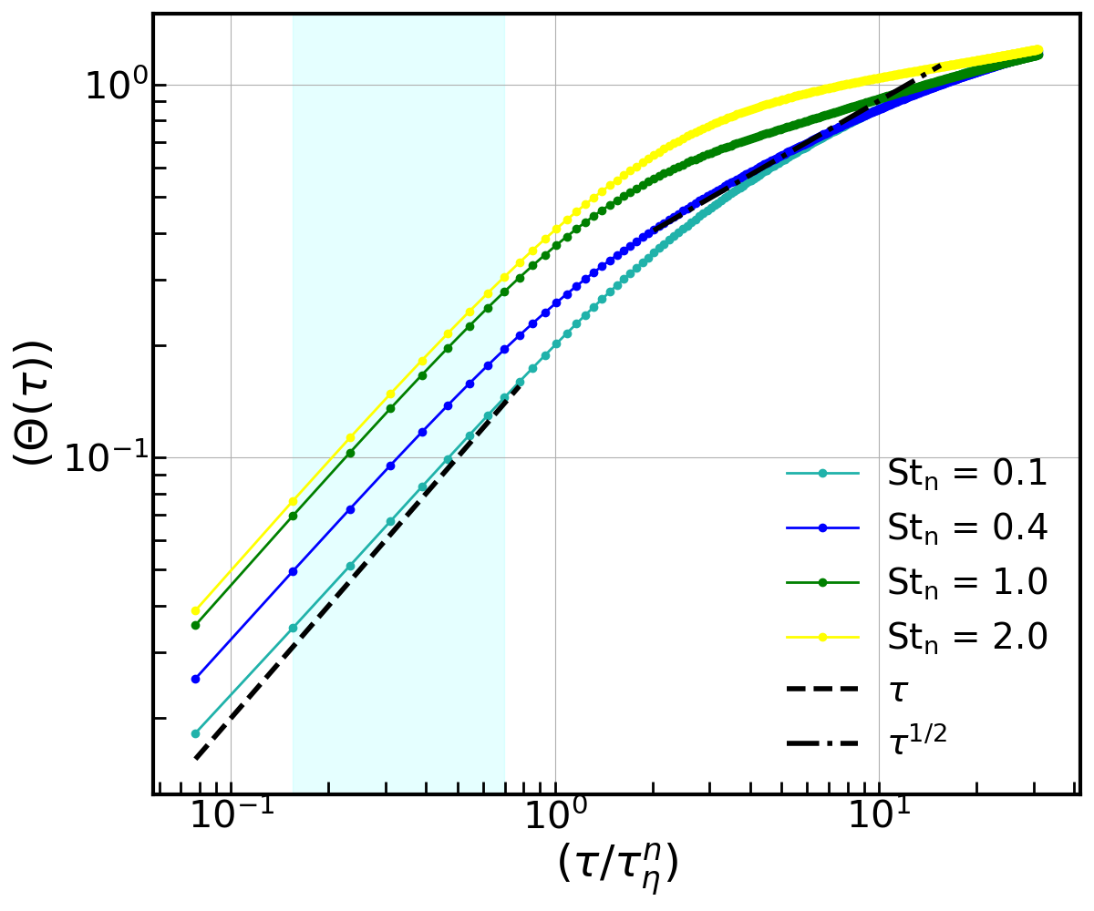
Figure 5: Log-log plots of the angle $\Theta(\tau)$ (see text) versus the time lag $\tau$ for (a) coflow ST at $T=1.65K$, (b) and (c) counterflow ST at $T=1.65K$ and $T=2.1K$ respectively. These plots are for $\beta=1.25$ and for different values of $\rm St_{n}$. Note the power-law scaling regions in the dissipation ranges (cyan-shaded regions) and in the inertial ranges (green-shaded regions) with $\Theta(\tau)\sim\tau^{\alpha}$ and $\Theta(\tau)\sim\tau^{\zeta}$, respectively.

III.3 Particle Trajectories

In addition to the statistics of particle velocities and accelerations in coflow and counterflow ST, it is instructive to examine the statistics of the trajectory curvature $\kappa$ and the modulus $\theta$ of the torsion. Both of these quantities have dimensions of inverse length, so large values of $\kappa$ and $\theta$ provide information about small-scale structures. To characterize the geometry of a particle’s trajectory we follow Ref. Akshay2014 and use the tangent ${\bf t}$, normal ${\bf n}$, and bi-normal $\bf b$ that are defined as Spivak1970 ; Stone2009 ; Braun2006

$${\bf t}=\frac{d{\bf r}}{ds};\quad{\bf n}=\frac{1}{\kappa}\frac{d{\bf t}}{ds};\quad{\bf b}={\bf t}\times{\bf b}.$$ (16)

Here, $s$ is the arc length and $\kappa$ is the curvature of the trajectory; ${\bf t},{\bf n}$, and ${\bf b}$ evolve as follows:

$$\frac{d{\bf t}}{ds}=\kappa{\bf n};\quad\frac{d{\bf n}}{ds}=\vartheta{\bf b}-\kappa{\bf t};\quad\frac{d{\bf b}}{ds}=-\vartheta{\bf n};$$ (17)

$\vartheta$ is the torsion of the trajectory. In terms of ${\bf v}$ and its derivatives ($\dot{\bf v},\ddot{\bf v}$), we have, in parametric form:

$$\kappa=\frac{\left|{{\bf v}\times\dot{\bf v}}\right|}{{\left|{\bf v}\right|}^{3}}=\frac{a_{n}}{v^{2}};\quad\vartheta=\frac{{\bf v}\cdot(\dot{\bf v}\times\ddot{\bf v})}{({\bf v}\cdot{\bf v})^{3}\kappa^{2}}.$$ (18)

where $v$ and $a_{n}$ are the magnitude of the velocity and of the normal component of particle’s acceleration.

In the log-log plots of Figs.6(a) and (b), we present for coflow ST, the CPDFs $Q(\kappa)$ and $Q(\theta)$, respectively, where $\theta=|\vartheta|$. Both these CPDFs show power-law-scaling regions: $Q(\kappa)\sim\kappa^{-h_{\kappa}+1}$, for $\kappa\rightarrow\infty$, with $h_{\kappa}\simeq 2.5$, i.e., the PDF $P(\kappa)\sim{\kappa}^{-h_{\kappa}}$; and $Q(\theta)\sim\theta^{-h_{\theta}+1}$, for $\theta\rightarrow\infty$, with $h_{\theta}\simeq 3$, i.e., the PDF $P(\theta)\sim{\theta}^{-h_{\theta}}$. In Figs. 6(c) and (d) we present, for counterflow ST, the CPDFs $Q(\kappa)$ and $Q(\theta)$, respectively. The exponents $h_{\kappa}$ and $h_{\theta}$ are the same as for coflow ST. We use a local-slope analysis (see, e.g., Ref.  Perlekar2011 ) to calculate the mean values of $h_{\kappa}$ and $h_{\theta}$ and their error bars (insets of Figs.6(a) and (b)). The exponents $h_{\kappa}$ and $h_{\theta}$, for the tails $P(\kappa)$ and $P(\theta)$ are universal, insofar as they are independent of $B,B^{\prime},\rho_{n},\rho_{s},\rm{St_{n}}$, $\rm{St_{n}}$, and $\widetilde{U}_{ns}$. The exponents $h_{\kappa}$ and $h_{\theta}$ have the same values as they do in classical-fluid turbulence Xu2007 ; Scagliarini2011 ; Akshay2014 .

We can obtain $h_{\kappa}$ and $h_{\theta}$, by making plausible approximations, as in classical-fluid turbulence Xu2007 ; Scagliarini2011 . For the curvature

$$P(\kappa)=\int\delta(\kappa-\frac{a_{n}}{v^{2}})\mathcal{P}(a_{n},v)da_{n}dv,$$ (19)

where $a_{n}$ is the normal component of the particle’s acceleration and $v$ the magnitude of its velocity. Furthermore, $\theta=\frac{|{\bf v}\cdot(\dot{\bf v}\times\ddot{\bf v})|}{({\bf v}\cdot{\bf v})^{3}\kappa^{2}}$, which we can simplify to obtain $\theta=\frac{|\ddot{\bf v}\cdot b|}{a_{n}v}$; large values of $\theta$ corresponding to small vaules of $a_{n}$ or $v$. For the modulus of the torsion

$$P(\theta)=\int\delta(\theta-\frac{1}{a_{n}v})\mathcal{P}(a_{n},v)da_{n}dv.$$ (20)

$a_{n}$ is a small-scale quantity and $v$ is dominated by large-scale flows, so we argue, as in Ref. Akshay2014 , that this scale separation suggests Xu2007 ; Scagliarini2011 ; Akshay2014 that we have the following factorization of the joint PDF:

$$\mathcal{P}(a_{n},v)\simeq P_{a_{n}}(a_{n})P_{v}(v).$$ (21)

From our DNSs of the 3D HVBK model we find that: (a) the PDF of $v$ is well approximated by the Maxwellian

$$P_{v}(v)=C_{1}v^{d-1}\exp(-v^{2}/C_{2}),$$ (22)

where $C_{1}$ and $C_{2}$ do not depend on $v$; and (b) the PDF of $a_{n}$ can be fit to the form

$$P_{a_{n}}(a_{n})=C_{3}a_{n}\exp(-a_{n}^{2}/C_{4}),$$ (23)

where $C_{3}$ and $C_{4}$ do not depend on $a_{n}$. By substituting Eqs. (21)-(23) in Eqs.(19) and (20), we get, after some simplification (in the small $a_{n}$ limit),

$$P(\kappa) \sim \kappa^{-2.5},\kappa\rightarrow\infty,$$

$$P(\theta) \sim \theta^{-3},\theta\rightarrow\infty;$$ (24)

our DNS results are in agreement with these power-law forms.

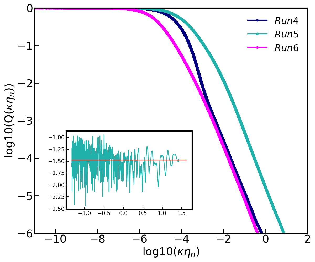
Figure 6: Log-log plots of CPDFs of (a) the curvature $\kappa$ and (b) the magnitude $\theta$ of the torsion of particle trajectories for coflow ST (runs ${\bf R1}$, ${\bf R2}$, and ${\bf R3}$); (c) and (d) are, respectively, the counterflow-ST counterparts of (a) and (b) (for runs ${\bf R5}$, ${\bf R6}$). Insets show plots of the local slopes of the tails of these CPDFs for run ${\bf R1}$ (in (a) and (b)) and for run ${\bf R5}$ (in (c) and (d)); the mean values of these local slopes yield the exponents of the power-law tail of the CPDFs (and the local-slope standard deviations give the error-bars for these exponents). [We can also calculate the exponent of the tail of the CPDF of $\kappa$ from the instantaneous angles of particle trajectories (see the Fig.S12 in Supplementary Material V).] In these plots $\rm{St_{n}}=1.0$ and $\beta=0.88$.

III.4 Energy Increments and the Irreversibility of 3D HVBK Turbulence

We turn now to the energy increments of inertial particles advected by 3D HVBK turbulent flows:

$$W(\tau)=\langle E_{(t_{0}+\tau)}-E_{(t_{0})}\rangle_{t_{0}},$$ (25)

where $E_{t}=(1/2){\bf v}(t)^{2}$ is the kinetic energy per unit mass of the particle and the particle velocity v is calculated by using Eqs.5; $\langle\rangle_{t_{0}}$ denotes the average over the time origin $t_{0}$. Such energy increments have been used to study irreversibility in classical-fluid turbulence, where it has been found that inertial particles, in turbulent flows of a classical fluid, gain energy slowly but lose it rapidly Akshay2018 ; Xu2014 ; such gain and loss are also referred to as flight-crash events because, on average, a particle decelerates faster than it accelerates. In Figs. 7(a) and (c), we plot, respectively, the PDFs ${\rm P}({W}/\sigma_{W})$, where $\sigma_{W}$ is the standard deviation, for coflow ST and counterflow ST at $T=1.65K$ and for light particles ($\beta=1.25$).

For coflow ST, we observe that ${\rm P}({W}/\sigma_{W})$ is negatively skewed for the small values of $\tau$, which indicates that the particles lose energy faster than they gain it. This skewness decreases as we increase $\tau$, as we show in blue curve of Fig. 7(a) for coflow ST; clearly, these PDFs are more symmetrical (and somewhat close to Gaussian PDFs) than their small-$\tau$ counterparts in Fig. 7(a).

There is a striking difference if we consider light particles ($\beta=1.25$) in counterflow ST (Fig. 7(c)): The skewness of ${\rm P}({W}/\sigma_{W})$ is positive (as has been found recently in a model for bacterial turbulence bacterial_turb ). We conjecture that this positive skewness arises because, in counterflow ST, the mean velocity $\tilde{U}_{ns}$ makes light particles cluster near large vortical structures [Fig.1(d)].

In Figs. 7(b) and 7(d), we present, for coflow ST and counterflow ST, respectively, and for different values of $\rm{St_{n}}$, graphs of the scaled third moment of the energy increment $<{W}^{3}/{E}^{3}_{nf}>$ versus the scaled time increment $\tau/\tau^{n}_{\eta}$, where ${E}_{nf}$, and $\tau^{n}_{\eta}$ are, respectively, the energy and the dissipation time scale for the normal fluid. From Figs. 7 (b) and (d), we infer that this third moment is negative for coflow ST but positive for counterflow ST. For small time increments in coflow ST

$$-<{W}^{3}/{E}^{3}_{nf}>\sim(\tau/\tau^{n}_{\eta})^{3};$$ (26)

and for counterflow ST

$$<{W}^{3}/{E}^{3}_{nf}>\sim(\tau/\tau^{n}_{\eta})^{3};$$ (27)

deviations from these simple-scaling form are evident at large values of $\tau/\tau^{n}_{\eta}$.

Flight-crash events have also been studied for coflow ST and thermal-counterflow ST in experiments with superfluid ⁴He, by using particles that are like Lagrangian tracers Mantia2019 . These experiments find that, on scales larger than the mean inter-vortex spacing and for mechanically driven coflow ST, there are negatively skewed PDFs ${\rm P}({W}/\sigma_{W})$, which are signatures of flight-crash events (see above); these experimental results are in consonance with our findings for coflow ST (Figs. 7(a-b)). Experiments Mantia2019 have also shown that the flight-crash events are less apparent in counterflow ST than in coflow ST; and there are signatures of positively skewed velocity-difference PDFs as well; this is in agreement with our results [Figs. 7(c-d)] for light particles. Furthermore, these experiments Mantia2019 find that,on scales smaller than or comparable to the mean inter-vortex spacing, there is less evidence for flight-crash events than in classical-fluid turbulence; we cannot address this here because, as we have noted above, the HVBK model cannot be used for a description of superfluid turbulence on length scales smaller than or comparable to the mean inter-vortex spacing. But even in this model of HVBK, the results of counterflow are strikngly different from that of coflow.

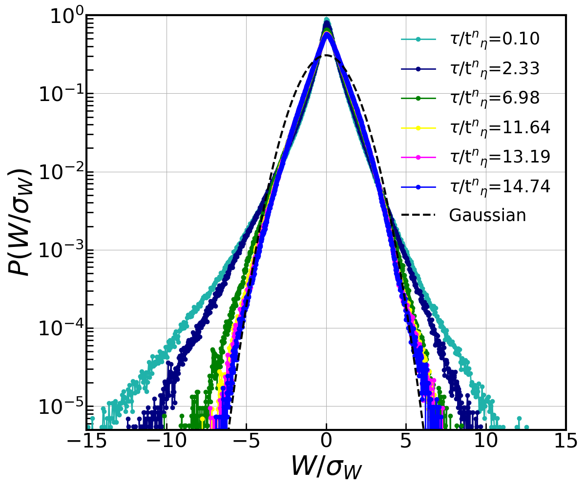
Figure 7: Semilog plots of the energy-increment PDF ${\rm P}(W/\sigma_{W})$, where $\sigma_{W}$ is the standard deviation of $W$, for coflow ST (columns 1-2) and for counterflow ST (columns 3-4) at $T=1.65K$: (a) for different time lags $\tau/t^{n}_{\eta}$, where $t^{n}_{\eta}$ is the normal-fluid dissipation time; (b) log-log plots of $\langle-W^{3}/E^{n}_{\rm nf}\rangle$ versus the time lag $\tau/t^{n}_{\eta}$, where $E^{n}_{\rm nf}$ is the normal-fluid energy, and $\tau^{3}$ is indicated by the black-dashed line. (c) and (d), are the counterflow-ST versions of (a) and (b), respectively. The cyan-shaded regions show the regimes over which we fit power laws. The dashed curve in (a) shows the Gaussian fits for ${\rm P}(W/\sigma_{W})$ for $\tau/t^{n}_{\eta}=14.74$ with $0$ mean and unit standard deviation. For all the plots $\rm St_{n}=1.0$ and $\beta=0.88$.

To quantify the irreversibility of the flow, we can calculate the power $p(t)={\bf a}(t)\cdot{\bf v}(t)$, from particle trajectories, with ${\bf a}=d{\bf v}/dt$ being the particle’s acceleration. The irreversibility parameter is, as in classical-fluid turbulence Akshay2018 ,

$${\rm Ir}=\frac{<p^{3}>}{<p^{2}>^{3/2}},$$ (28)

which we plot versus $\rm{St_{n}}$ in Figs. 8(a) and (b) for coflow and counterflow ST, respectively, at $T=1.65K$ and for both light and heavy particles. For coflow ST, this irreversibility parameter is negative for light ($\beta=1.25$) as well as heavy ($\beta=0.1$) particles and for all $\rm{St_{n}}$; this has also been found in classical-fluid turbulence Akshay2018 . Moreover, it has been argued pumir2016 that ${\rm Ir}<0$ in 3D fluid turbulence; similar arguments can be used, mutatis mutandis, to conclude that ${\rm Ir}<0$ in 3D HVBK coflow turbulence, in agreement with our graphs in Fig. 8(a). For counterflow ST the irreversibility parameter [Fig.8(b)] is positive for light particles ($\beta=1.25$), which reflects the positive skewness in the energy increments of Fig.7(c)-(d); in contrast, for heavy particles ($\beta=0.1$), the irreversibility parameter is negative [navy-blue curve in Fig.8(b)], which indicates negatively skewed PDFs of energy increments.

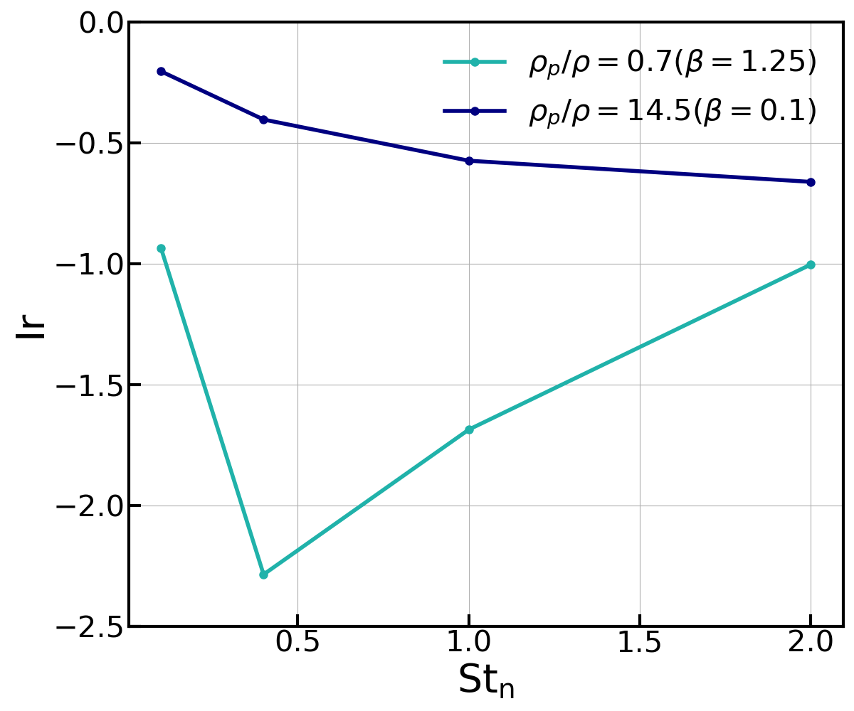
Figure 8: Plots of the irreversibility parameter ${\rm Ir}$ (see text) versus ${\rm St_{n}}$ for (a) coflow ST and (b) counterflow ST . These plots are at $T=1.65K$ and for $\beta=0.1$ in navy color and for $\beta=1.25$ in lightseagreen.

IV Conclusions

Studies of inertial particles in superfluid turbulence are in their infancy; by contrast, there have been extensive studies of the statistical properties of such particles advected by classical-fluid turbulence Toschi2009 ; Bec2005 . Hence, we have carried out a systematic study of inertial particles in statistically steady coflow ST and counterflow ST in the 3D HVBK model, for different values of the Stokes numbers $\rm{St_{n}}$, with normal-fluid fractions and mutual-friction coefficients that are taken from measurements Donnelly1998 on superfluid ⁴He, as a function of the temperature. One recent study Giorgio2020 has investigated the clustering of inertial particles in 3D HVBK turbuence and has shown that, for coflow ST, although the particle distribution is nearly uniform at high temperatures, it still has signatures of some clustering.

Coflow ST is isotropic but counterflow ST is inherently anisotroic; we have shown this via isosurfaces of $|\omega_{n}|$ and the positions of representative particles in Fig. 1. For coflow ST at $T=1.65K$, particles cluster as they do in classical-fluid turbulence because, at this temperature, the mutual friction couples both fluids strongly. The particles form large-scale clusters at $T=1.65K$ in counterflow ST; and light particles are attracted towards [Fig. 1 (d)] the large vortical columns; by contrast, heavy particles are expelled from these vortical columns [Fig. 1(c)].

These large vortical columns have a direct influence on the statistics of the angle $\Theta$, which is the angle between subsequent inertial-particle-displacement increment. The study of $\Theta$ reveals two scaling regions; one in dissipation and other in the inertial region. In case of coflow ST, the large time asymptotic value of $\Theta$ is the same for all Stokes number which is the signature of isotropic case Bos2015 . While for counterflow this asymptotic value of $\Theta$ reduces for light particles with large $\rm St_{n}$ as they are affected more by the confinement from normal fluid component. Ref confinement studies the effect of mean velocity on the angle $\Theta$ in case of classical turbulence and also observe such reduction in the large time lag value of $\Theta$.

One of the main results of this study is the signature of positive skewness in the PDFs of energy increment 7(c)-(d) for light particles. As we mention earlier, in a recent study of coflow and counterflow ST, Ref Mantia2019 observe that the flight crash events are less prominent than that of classical fluid turbulence; they show that for coflow there is some similarity to classical case at large length scales. This result of coflow is in agreement with our study .i.e there are signatures of flight crash events in HVBK model of coflow. For counterflow, Ref Mantia2019 observe different results from the classical case at all length scales and found signatures of positive skewness in moments of velocity differences. This is also in consonance with our results of positive skewness in case of counterflow for light particles; while for heavy particles the PDFs of energy increment 7 are negatively skewed.

We hope that our definition and study of flight crash events, for inertial particles in 3D HVBK turbulence, will lead to new experimental investigations of this problem in, e.g., superfluid ⁴He or Bose-Einstein condensates (BECs).

V Supplementary Material

In the Supplementary Material, we provide: (1) a brief description of the specific power laws found in Fig. 2; (2) iso-surface plots of the magnitude of the normal-fluid vorticity $|\omega_{n}|$ at temperature $T=2.10K$; (3) CPDFs of the persistence time III.1, $t_{s}^{per}$, at $T=1.65K$ for the superfluid component; (4) the curvature III.3, $\kappa$, of particle trajectories, obtained from the instantaneous angle $\Theta(t,\tau)$; (5) iso-surface plots of the magnitude of the normal-fluid vorticity $|\omega_{n}|$ at temperature $T=2.10K$ for a square cuboid domain with resolution $256\times 256\times 1024$.

VI Appendix

Variable	Description
$\tau_{\eta}^{n/s}$	Kolmogorov-dissipation time scale for normal fluid/superfluid
${\bf U_{ns}}(\widetilde{U}_{ns})$	Counterflow mean velocity (magnitude of mean relative velocity)
$\beta$	Parameter that accounts for the added mass effect to the particle
$\rho_{p}$	Particle’s density
$\Theta$	Angle between particle’s subsequent position increment
$\alpha,\zeta$	exponents of the angle $\Theta$
$\kappa$	Curvature of the particle’s trajectory
$\theta$	Magnitude of the torsion of the particle’s trajectory
$Q_{n/s},R_{n/s}$	Invariants of velocity gradient tensor for normal-fluid/superfluid
$t^{per}_{n/s}$	Persistence time of particles for normal-fluid/superfluid
$W(\tau)$	Particle’s kinetic energy increment separated by time lag $\tau$
$p$	Power input to the particle
Ir	Irreversibility

Table 2: Table consisting of all the variables used in the paper along with their descriptions.

AUTHOR DECLARATIONS

Conflict of Interest

The authors have no conflicts to disclose.

Data Availability

The data that support the findings of this study are available from corresponding author upon reasonable request.

VII Supplementary Material

In this Supplemental Material, we provide the following:

1. Specific powers laws in counterflow: These specific powers are standard in the study of statistically homogeneous isotropic turbulence in the phenomenology of Kolmogorov-1941 (K41) theory. At the level of K41, the energy spectrum $E(k)\sim k^{-5/3}$; this energy spectrum is obtained when we average over spherical shells in $k$-space (by using an isotropic version of Eq. (9) in the main paper). Given the inherent anisotropy of counterflow ST, the energy spectrum is a function of $k_{\parallel}$ and $k_{\perp}$, which are the wavevectors along the counterflow direction and perpendicular to it, respectively (see the definitions below Eq. (9) in the main paper). In the perpendicular plane, we average over circular shells (the second line of Eq. (9)); this yields an energy spectrum $\sim k_{\perp}^{-8/3}$ (at the level of K41 arguments); similarly, in the one-dimensional parallel direction, the energy spectrum $\sim k_{\parallel}^{-11/3}$ (at the level of K41 arguments); the spectral exponent is $-5/3$, for a spherical average, $-8/3$, for a circular average, and $-11/3$ along one direction (at the level of K41 arguments). This is in agreement with the recent results of Ref. [36] as we have mentioned clearly in the main paper.

2. In Fig. S10 we show the isosurface plots of the magnitude of the super-fluid vorticity $|\omega_{s}|$ at $T=2.10K$ for counterflow ST and $\widehat{\bf U}_{ns}=\widehat{e}_{k}$ (run R6).

   

   

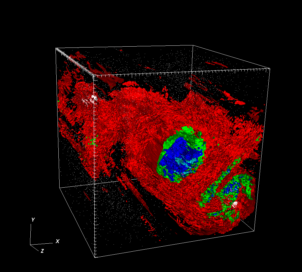
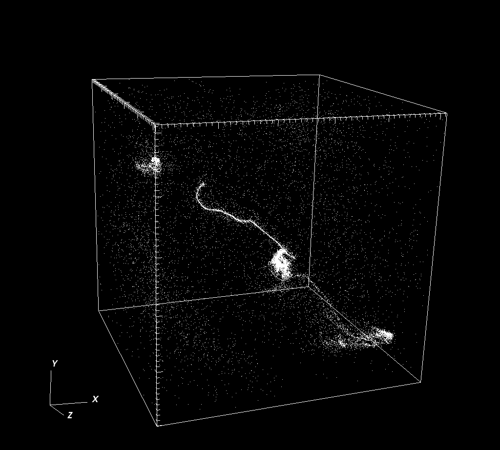
   Figure S10: Isosurface plots of the magnitude of the super-fluid vorticity $|\omega_{s}|$, for counterflow ST , $\widehat{\bf U}_{ns}=\hat{e_{k}}$, and $T=2.10$K. We indicate by small white spheres the positions of particles (with $\rm St_{n}=1.0$). Column2 and column3 show the positions of light ($\beta=1.25$) and heavy ($\beta=0.1$) particles respectively.

3. We plot the cumulative probability distribution functions (CPDFs) of the persistence times (see the main paper) in the Eulerian frame for the superfluid component; for coflow ST in Fig.S11(a) and for counterflow ST in Fig.S11(b).
   

   

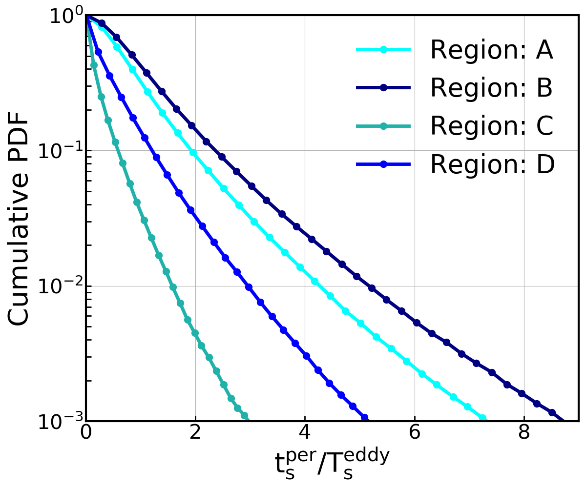
   Figure S11: Semilog plots of the CPDFs of the persistence times, $t^{per}_{n}$, in the Eulerian frame for the superfluid ($s$) component; for coflow ST in (a) and for counterflow ST in (b).

VIII Appendix

We can also calculate the curvature of particle trajectories from the instantaneous angle $\Theta(t,\tau)$. The curvature of particle trajectories at time t for small time lag $\tau$ in terms of instantaneous angle $\Theta(t,\tau)$ Bos2015 is

$$\kappa(t)=\lim_{\tau\to 0}\frac{\left|\Theta(t,\tau)\right|}{2\tau\|v(t)\|}.$$ (29)

Log-log plots of these CPDFs are shown in Fig. LABEL:fig:append. The slope of the tail of CPDFs are 2.5 and it is same as calculated in the main part of this article. Here, We have calculated the slope of curvature in y-range from -2.0 to -4.5.

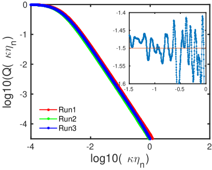
Figure S12: Log-log plots of CPDFs of the curvature $\kappa$ of particle trajectories, calculated from the instantaneous angle $\Theta(t,\tau)$, at time $t$ for the time lag $\tau$ from runs $\bf{R1}$, $\bf{R2}$, and ${\bf R3}$. The inset shows a plot of the the local slopes of the tail of the CPDF for $\bf{R1}$; the mean value of these local slopes gives the exponent of the power-law tail of the CPDF and the standard deviations are the error-bars for the exponents. These above plots are for $\rm{St_{n}}=0.1$.

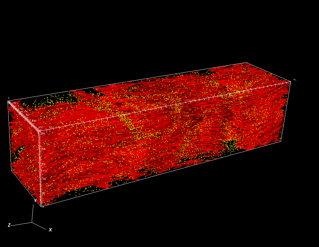
Figure S13: Isosurface plots of the magnitude of the normal-fluid vorticity at $|\omega_{n}|$, for counterflow ST for a square cuboid simulation domain with $256\times 256\times 1024$ collocation points, $\widehat{\bf U}_{ns}=\hat{e_{k}}$, and $T=2.10$K. We indicate by small yellow spheres the positions of particles (with $\rm St_{n}=1.0$).

References

- (1) R. A. Shaw, Annual Review of Fluid Mechanics 35, 183 (2003).
- (2) W. W, Grabowski and L. P. Wang, Annual Review of Fluid Mechanics 45, 293 (2013).
- (3) G. Falkovich, A. Fouxon, and M. Stepanov, Nature, London 419, 151 (2002).
- (4) P. J. Armitage,Astrophysics of Planet Formation (Cambridge University Press, Cambridge, UK 2010).
- (5) J. Eaton and J. Fessler, Intl. J. Multiphase Flow 20, 169 (1994).
- (6) S. Post and J. Abraham, Intl. J. Multiphase Flow 28, 997 (2002).
- (7) J. Cardy, G. Falkovich and K. Gawedzki, Non-equilibrium Statistical Mechanics and Turbulence (Cambridge University Press, Cambridge, 2008)
- (8) R. J. Donnelly, Quantized Vortices in Helium II (Cambridge University Press, Cambridge, 1991).
- (9) M. S. Paoletti and D. P. Lathrop, Annu. Rev. Condens. Matter Phys. 2, 213 (2011).
- (10) L. Skrbek and K. R. Sreenivasan, Phys. Fluids 24, 011301 (2012).
- (11) N. G. Berloff, M. Brachet, and N. P. Proukakis, Proc. Natl. Acad. Sci. U.S.A. 111, 4675 (2014).
- (12) M. Tsubota, K. Fujimoto, and S. Yui, Numerical Studies of Quantum Turbulence, J Low Temp Phys, 188: 119 (2017). DOI: 10.1007/s10909-017-1789-8
- (13) C.F. Barenghi and N.G. Parker, A Primer on Quantum Fluids, SpringerBriefs on Physics (Springer, 2017); https://doi.org/10.1007/978-3-319-42476-7.
- (14) G.P. Bewley, D.P. Lathrop, and K.R. Sreenivasan, Nature 441, 588 (2006).
- (15) G.P. Bewley, M.S. Paoletti, K.R. Sreenivasan, and D.P. Lathrop, Proc. Natl. Acad. Sci. U.S.A. 105, 13707 (2008).
- (16) D. R. Poole, C. F. Barenghi, Y. A. Sergeev and W. F. Vinen, Phys. Rev. B 71, 064514 (2005).
- (17) M. La Mantia, D. Duda, M. Rotter and L. Skrbek, J. Fluid Mech. 717, R9 (2013)
- (18) M. La. Mantia and L. Skrbek, Phys. Rev. B 90, 014519 (2014).
- (19) D.E. Zmeev, F. Pakpour, P. M. Walmsley, A. I. Golov, W. Guo, D.N. McKinsey, G.G. Ihas, P.V.E. McClintock, S.N. Fisher, and W. F. Vinen, Phys. Rev. Lett. 110 175303 (2013).
- (20) W. Guo, M. La Mantia, D.P. Lathrop, and S.W.V. Sciver, Proc Natl Acad Sci USA 111 4653–4658 (2014).
- (21) Y. Tang, S. Bao, T. Kanai , and W. Guo, Statistical properties of homogeneous and isotropic turbulence in He II measured via particle tracking velocimetry, Phys. Rev. Fluids 5 084602 (2020).
- (22) P. Švančara and M. La Mantia, Flight-crash events in superfluid turbulence, J. Fluid Mech. 876, R2 (2019).
- (23) G. Krstulovic and M. Brachet, Phys. Rev. E 83, 066311 (2011).
- (24) V. Shukla, M. Brachet, and R. Pandit, Turbulence in the two-dimensional Fourier-truncated Gross–Pitaevskii equation, New J. Phys., 15: 113025, (2013). http://www.njp.org/doi: 10.1088/1367-2630/15/11/113025.
- (25) E. Zaremba, T. Nikuni, and A. Griffin, Journal of Low Temperature Physics 116: 277 (1999); https://doi.org/10.1023/A:1021846002995 .
- (26) T. Winiecki and C. S. Adams, Europhys. Lett. 52, 257 (2000).
- (27) V. Shukla, M. Brachet, and R. Pandit, Sticking transition in a minimal model for the collisions of active particles in quantum fluids, Phys. Rev. A (Rapid Communications), 94: 041602, (2016).
- (28) V. Shukla, R. Pandit, and M. Brachet, Particles and fields in superfluids: Insights from the twodimensional Gross-Pitaevskii equation, Phys. Rev. A, 97(1): 013627, 2018.
- (29) U. Giuriato and G. Krstulovic, Interaction between active particles and quantum vortices leading to Kelvin wave generation, Scientific Reports 9 (1), 4839 (2019).
- (30) U. Giuriato, G. Krstulovic, and D. Proment, Clustering and phase transitions in a 2D superfluid with immiscible active impurities, J. Phys. A: Math. Theor. 52, 305501 (2019).
- (31) U. Giuriato, G. Krstulovic, S. Nazarenko, How do trapped particles interact with and sample superfluid vortex excitations? arXiv:1907.01111v1 [cond-mat.other] (2019).
- (32) L. Biferale, D. Khomenko, V. L’vov, A. Pomyalov, I.Procaccia, and G. Sahoo, Phys. Rev. Lett. 122, 144501 (2019).
- (33) Dmytro Khomenko, Victor S. L’vov, Anna Pomyalov, and Itamar Procaccia, Phys. Rev. B 93, 014516 (2016).
- (34) J.I. Polanco and G. Krstulovic Phys. Rev. Lett. 125, 254504 (2020).
- (35) VS L’vov, YV Lvov, S Nazarenko, A Pomyalov, arXiv preprint arXiv:2106.07014 (2021).
- (36) C.F. Barenghi, L. Skrbek, and K.R. Sreenivasan, Proc. Natl. Acad. Sci., 111, 4647-4652 (2014).
- (37) J.I. Polanco, and G. Krsutlovic, Phys. Rev. Fluids 5, 032601(R) (2020)
- (38) F. Toschi and E. Bodenschatz, Annual Review of Fluid Mechanics, 41, 375 (2009).
- (39) J. Bec, J. Fluid Mech. 528 255 (2005).
- (40) R.J. Donnelly, J. Phys. Condensed Matter 11, 7783 (1999).
- (41) C.F. Barenghi, R.J. Donnelly, and W.F. Vinen, J. Low Temp. Phys. 52, 189 (1983).
- (42) H.E. Hall and W.F. Vinen, Proc. Roy. Soc. A 238, 215 (1956).
- (43) I.M. Khalatnikov, An Introduction to the Theory of Superfluidity (WA Benjamin, New York, 1965).
- (44) P.E. Roche, C.F. Barenghi, and E. Lévêque, Europhys. Lett. 87, 54006 (2009).
- (45) V. Shukla, A. Gupta and R. Pandit, Phys. Rev. B 92, 104510 (2015)
- (46) L. Biferale, D. Khomenko, V. L’vov, A. Pomyalov, I. Procaccia, and G. Sahoo, Phys. Rev. Lett. 122, 144501 (2019); L. Biferale, D. Khomenko, V. S. L’vov, A. Pomyalov, I. Procaccia, and G. Sahoo, Phys. Rev. Fluids 3, 024605 (2018).
- (47) A.K. Verma, V. Shukla, A. Basu, R. Pandit, arXiv preprint arXiv:1905.01507 (2019).
- (48) W. F. Vinen, Proc. R. Soc. London, Ser. A 242 493 (1957).
- (49) F. Toschi, L. Biferale, G. Boffeta, A. Celani, B. J. Devenish and A. Lanotte, J. Turbul. 6 No. 15, (2005).
- (50) L. Biferale, G. Boffeta, A. Celani, A. Lanotte, and F. Toschi Phys. Fluids 6 No. 15, (2005).
- (51) Benzi, R., Ciliberto, S., Tripiccione, R., Baudet, C., Massaioli, F. and Succi, S.Extended self-similarity in turbulent flows. Phys. Rev. E 48, R29–R32 (1993);
- (52) W.F. Vinen and J. J. Niemela. Quantum turbulence. J. Low Temp. Phys., 128(5-6):167–231, 2002.
- (53) V.S. L’vov, S.V. Nazarenko, and O. Rudenko, Phys. Rev. B 76, 024520 (2007).
- (54) K. Morris, J. Koplik, and D.W.I. Rouson, Phys. Rev. Lett. 101,015301 (2008).
- (55) D.H. Wacks and C.F. Barenghi, Phys. Rev. B 84, 184505 (2011).
- (56) C. Canuto, M.Y. Hussaini, A. Quarteroni, and T.A. Zang, Spectral Methods in Fluid Dynamics (Springer- Verlag, Berlin, 1988).
- (57) D. Gottlieb, and S. A. Orszag, Numerical Analysis of Spectral Methods (SIAM, Philadelphia, 1977).
- (58) https://www.fftw.org/
- (59) A.G. Lamorgese, D.A. Caughey, and S.B. Pope, Phys. Fluids 17, 015106 (2005).
- (60) G. Sahoo, P. Perlekar, and R. Pandit, New J. Phys. 13, 0130363 (2011).
- (61) R.J. Donnelly and C.F. Barenghi, J. Phys. Chem. Ref. Data 27, 1217 (1998).
- (62) Boué, Laurent et.al., Phys. Rev. B, 91, 144501(1998)
- (63) R. Gatignol, Journal de Mécanique Théorique et Ap- pliquée 2.2, 143 (1983).
- (64) M.R. Maxey and J.J. Riley, Physics of Fluids 26.4 883 (1983): 883-889.
- (65) J. Bec, et al., Phys. Fluids 18, 091702 (2006).
- (66) W.J.T. Bos, B. Kadoch, K. Schneider, Phys. Rev. Lett. 114 214502 (2015)
- (67) X. He, S. Apte, K. Schneider, B. Kadoch, and M. Farge Center for Turbulence Research Proceedings of the Summer Program (2016). year=2016, volume=18, pages=113047
- (68) A. Bhatnagar, A. Gupta, D. Mitra, P. Perlekar, M. Wilkinson, and R. Pandit, Phys. Rev. E 94, 063112 (2016).
- (69) M. Spivak, (1979). A comprehensive introduction to dif- ferential geometry, vol. 1-5. I (Boston, Mass., 1970).
- (70) M. Stone, and P. Goldbart, Mathematics for physics: a guided tour for graduate students, (Cambridge Univer- sity Press 2009) p-242.
- (71) W. Braun, F. De Lillo, and B. Eckhardt, J. Turbul. 7, 1 (2006).
- (72) P. Perlekar, S.S. Ray, D. Mitra, and R. Pandit, Phys. Rev. Lett. 106, 054501 (2011).
- (73) H. Xu, N. T. Ouellette, and E. Bodenschatz, Phys. Rev. Lett., 98, 050201 (2007).
- (74) A. Scagliarini, Journal of Turbulence 12 (2011).
- (75) A. Bhatnagar, A. Gupta, D. Mitra, R. Pandit, and P. Perlekar, Phys. Rev. E 94, 053119 (2016).
- (76) Gomes-Fernandes, R., Ganapathisubramani, B., and Vassilicos, J., Journal of Fluid Mechanics, 756, 252-292, (2014).
- (77) A. Bhatnagar, A. Gupta, D. Mitra, and R. Pandit, Heavy inertial particles in turbulent flows gain energy slowly but lose it rapidly, Phys. Rev. E 97, 033102 (2018).
- (78) H. Xu, A. Pumir, G. Falkovich, E. Bodenschatz, M. Shats, H. Xia, N. Francois, and G. Boffetta, Flight-crash events in turbulence, Proc. Natl. Acad. Sci. USA 111, 7558 (2014).
- (79) Kolluru Venkata Kiran et. al, arXiv:2201.12722.
- (80) Pumir, Alain and Xu, Haitao and Bodenschatz, Eberhard and Grauer, Rainer, Phys. Rev. Lett., 116, 124502 (2016).