Offline Reinforcement Learning with Value-based Episodic Memory

Abstract

Offline reinforcement learning (RL) shows promise of applying RL to real-world problems by effectively utilizing previously collected data. Most existing offline RL algorithms use regularization or constraints to suppress extrapolation error for actions outside the dataset. In this paper, we adopt a different framework, which learns the $V$-function instead of the $Q$-function to naturally keep the learning procedure within the support of an offline dataset. To enable effective generalization while maintaining proper conservatism in offline learning, we propose Expectile $V$-Learning (EVL), which smoothly interpolates between the optimal value learning and behavior cloning. Further, we introduce implicit planning along offline trajectories to enhance learned $V$-values and accelerate convergence. Together, we present a new offline method called Value-based Episodic Memory (VEM). We provide theoretical analysis for the convergence properties of our proposed VEM method, and empirical results in the D4RL benchmark show that our method achieves superior performance in most tasks, particularly in sparse-reward tasks.

1 Introduction

Despite the great success of deep reinforcement learning (RL) in various domains, most current algorithms rely on interactions with the environment to learn through trial and error. In real-world problems, particularly in risky and safety-crucial scenarios, interactions with the environment can be expensive and unsafe, and only offline collected datasets are available, such as the expert demonstration or previously logged data. This growing demand has led to the emergence of offline reinforcement learning (offline RL) to conduct RL in a supervised manner.

The main challenge of offline RL comes from the actions out of the dataset’s support (Kumar et al., 2019; 2020). The evaluation of these actions that do not appear in the dataset relies on the generalization of the value network, which may exhibit extrapolation error (Fujimoto et al., 2019). This error can be magnified through bootstrapping, leading to severe estimation errors. A rapidly developing line of recent work (Fujimoto et al., 2019; Kumar et al., 2020; Ghasemipour et al., 2021; Yang et al., 2021) utilizes various methods to constrain optimistic estimation on unseen actions, such as restricting available actions with a learned behavior model (Fujimoto et al., 2019) or penalizing the unseen actions with additional regularization (Kumar et al., 2020).

Another line of methods, on the contrary, uses the returns of the behavior policy as the signal for policy learning, as adopted in (Wang et al., 2018; Peng et al., 2019; Chen et al., 2020). By doing so, they keep the whole learning procedure within the dataset’s support. However, the behavior policy of the dataset can be imperfect and insufficient to guide policy learning. Learning optimal values within the dataset, on the other extreme, can lead to erroneously optimistic value estimates since data is limited and off-policy. To achieve a trade-off between imitation learning and optimal value learning, we propose Expectile $V$-learning (EVL), which is based on a new expectile operator that smoothly interpolates between the Bellman expectation operator and optimality operator.

To better solve long-horizon and sparse-reward tasks, we further propose using value-based planning to improve the advantage estimation for policy learning. We adopt an implicit memory-based planning scheme that strictly plans within offline trajectories to compute the advantages effectively, as proposed in recent advances in episodic memory-based methods (Hu et al., 2021). Together, we present our novel framework for offline RL, Value-based Episodic Memory (VEM), which uses expectile $V$-learning to approximate the optimal value with offline data and conduct implicit memory-based planning to further enhance advantage estimation. With the properly learned advantage function, VEM trains the policy network in a simple regression manner. We demonstrate our algorithm in Figure 1, and a formal description of our algorithm is provided in Algorithm 1.

Figure 1: The diagram of algorithms. The left side denotes the general $Q$-based offline RL methods. The right side is the framework of our proposed approach (VEM). Q-based methods learns bootstrapped $Q$-values, but requires additional constraint or penalty for actions out of the dataset. Our method, on the contrary, learns bootstrapped $V$-values while being completely confined within the dataset without any regularization.

The contributions of this paper are threefold. First, we present a new offline $V$-learning method, EVL, and a novel offline RL framework, VEM. EVL learns the value function through the trade-offs between imitation learning and optimal value learning. VEM uses a memory-based planning scheme to enhance advantage estimation and conduct policy learning in a regression manner. Second, we theoretically analyze our proposed algorithm’s convergence properties and the trade-off between contraction rate, fixed-point bias, and variance. Specifically, we show that VEM is provably convergent and enjoys a low concentration rate with a small fixed-point bias. Finally, we evaluate our method in the offline RL benchmark D4RL (Fu et al., 2020). Comparing with other baselines, VEM achieves superior performance, especially in the sparse reward tasks like AntMaze and Adroit. The ablation study shows that VEM yields accurate value estimates and is robust to extrapolation errors.

2 Background

2.1 Preliminaries

We consider a Markov Decision Process (MDP) $M$ defined by a tuple $(\mathcal{S},\mathcal{A},P,r,\gamma)$, where $S$ is the state space, $A$ is the action space, $P(\cdot|s,a):\mathcal{S}\times\mathcal{A}\times\mathcal{S}\to\mathbb{R}$ is the transition distribution function, $r(s,a):\mathcal{S}\times\mathcal{A}\to\mathbb{R}$ is the reward function and $\gamma\in[0,1)$ is the discount factor. We say an environment is deterministic if $P(\cdot|s,a)=\delta(s^{\prime})$ for some $s^{\prime}$, where $\delta(\cdot)$ is the Dirac function. The goal of an RL agent is to learn a policy $\pi:\mathcal{S}\times\mathcal{A}\to\mathbb{R}$, which maximizes the expectation of a discounted cumulative reward: $\mathcal{J}(\pi)=\mathbb{E}_{s_{0}\sim\rho_{0},a_{t}\sim\pi(\cdot|s_{t}),s_{t+1}\sim P(\cdot|s_{t},a_{t})}\left[\sum_{t=0}^{\infty}\gamma^{t}r(s_{t},a_{t})\right]$, where $\rho_{0}$ denotes the distribution of the initial states.

2.2 Value-based Offline Reinforcement Learning Methods

Current offline RL methods can be roughly divided into two categories according to types of learned value function: $Q$-based and $V$-based methods. $Q$-based methods, such as BCQ (Fujimoto et al., 2019), learn $Q$-function for policy learning and avoid selecting unfamiliar actions via constraints or penalty. On the contrary, $V$-based methods (Peng et al., 2019; Siegel et al., 2020; Chen et al., 2020) learns the value of behavior policy $V^{\mu}(s)$ with the trajectories in the offline dataset $\mathcal{D}$ and update policy as a regression problem. Based on the learned $V$-function, $V$-based methods like AWR (Peng et al., 2019) updates the policy using advantage-weighted regression, where each state-action pair is weighted according to the exponentiated advantage

$$\max_{\phi}\mathcal{J}_{\pi}(\phi)=\mathbb{E}_{(s_{t},a_{t})\sim\mathcal{D}}\left[\log\pi_{\phi}(a_{t}\mid s_{t})\exp{\left(R_{t}-V^{\mu}(s_{t})\right)}\right].$$ (1)

3 Method

In this section, we describe our novel offline method, value-based episodic memory, as depicted in Figure 1. VEM uses expectile $V$-learning (EVL) to learn $V$-functions while avoiding extrapolation error in the action space. EVL uses an expectile operator that interpolates between Bellman expectation operator and optimality operator to balance behavior cloning and optimal value learning. Further, VEM integrates memory-based planning to improve the advantage estimation and accelerate the convergence of EVL. Finally, generalized advantage-weighted learning is used for policy learning with enhanced advantage estimation. A formal description for the VEM algorithm is shown in Algorithm 1 in Appendix A.1.

3.1 Expectile V-Learning

To achieve a balance between behavior cloning and optimal value learning, we consider the Bellman expectile operator defined as follows:

$$(\mathcal{T}^{\mu}_{\tau}V)(s)\coloneqq\operatorname*{arg\,min}_{v}\mathbb{E}_{a\sim\mu(\cdot\mid s)}{\left[\tau[\delta]^{2}_{+}+(1-\tau)[-\delta]^{2}_{+}\right]}$$ (2)

where $\mu$ is the behavior policy, $\delta=\mathbb{E}_{s^{\prime}\sim P(\cdot\mid s,a)}{\left[r(s,a)+\gamma V(s^{\prime})-v\right]}$ is the expected one-step TD error and $[\cdot]_{+}=\max(\cdot,0)$. This operator resembles the expectile statistics (Newey & Powell, 1987; Rowland et al., 2019) and hence its name. We can see that when $\tau=1/2$, this operator is reduced to Bellman expectation operator, while when $\tau\rightarrow 1$, this operator approaches Bellman optimality operator.

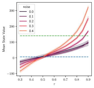
Figure 2: Trade-offs of EVL between generalization and conservatism in a random MDP. The green line shows the optimal value and the blue line shows the value of behavior policy. The curve is averaged over 20 MDPs.

We use the following toy example to further illustrate the trade-offs achieved by EVL. Consider a random generated MDP. When the operator can be applied exactly, the Bellman optimality operator is sufficient to learn the optimal value $V^{*}$. However, applying operators with an offline dataset raises a noise on the actual operator due to the estimation error with finite and biased data. We simulate this effect by adding random Gaussian noise to the operator. Applying the optimality operator on offline datasets can lead to severe overestimation due to the maximization bias and bootstrapping. The value estimation learned by EVL, on the contrary, achieves a trade-off between learning optimal policy and behavior cloning and can be close to the optimal value with proper chosen $\tau$, as depicted in Figure 2. The estimation error can be significant when the dataset is small, and EVL needs a smaller $\tau$ to be more conservative and closer to behavior cloning. When the dataset is large, the estimation error becomes small, and we can use a larger $\tau$ to recover the optimal policy.

However, the expectile operator in Equation 2 does not have a closed-form solution. In practice, we consider the one-step gradient expectile operator

$$({(\mathcal{T}_{g})}_{\tau}^{\mu}V)(s)=V(s)+2\alpha\mathbb{E}_{a\sim\mu(\cdot\mid s)}\left[\tau\left[\delta(s,a)\right]_{+}+(1-\tau)[\delta(s,a)]_{-}\right],$$ (3)

where $\alpha$ is the step-size. Please refer to Appendix B.1 for the detailed derivation. For notational convenience, we use ${\mathcal{T}}_{\tau}^{\mu}$ to denote the one-step gradient expectile operator ${(\mathcal{T}_{g})}_{\tau}^{\mu}$ hereafter.

In real-world problems, the dynamics are often nearly deterministic. We leverage this assumption and remove the expectation over the next states in the operator, which leads to Expectile $V$-Learning, where we train the value network to minimize the following loss:

$$\mathcal{J}_{V}(\theta) =\mathbb{E}_{(s_{t},a_{t},s_{t+1})\sim\mathcal{D}}\left[\left(\hat{V}(s_{t})-V_{\theta}\left(s_{t}\right)\right)^{2}\right],$$ (4)

$$\hat{V}(s) =V_{\theta^{\prime}}(s)+2\alpha\left[\tau\left[\delta(s,a,s^{\prime})\right]_{+}+(1-\tau)[\delta(s,a,s^{\prime})]_{-}\right],$$

where $\hat{V}$ is the target value after applying one-step gradient expectile operator and $\delta(s,a,s^{\prime})=r(s,a)+\gamma V_{\theta^{\prime}}(s^{\prime})-V_{\theta^{\prime}}(s)$. $V$-function and the target $\hat{V}$-function are parameterized by $\theta$ and $\theta^{\prime}$, respectively. EVL is guaranteed to converge with concentration rate $\gamma_{\tau}=1-2(1-\gamma)\alpha\max\{\tau,1-\tau\}$. Please refer to Section 4 for a detailed analysis.

3.2 Implicit Memory-Based Planning

Although EVL reduces the extrapolation error, it is still a challenging problem to bootstrap over long time horizons due to estimation errors with a fixed dataset. Therefore, we propose using value-based planning to conduct bootstrapping more efficiently. We adopt an implicit memory-based planning scheme that strictly plans within offline trajectories to avoid over-optimistic estimations in the planning phase. This is aligned with recent advances in episodic memory-based methods (Hu et al., 2021), but we conduct this planning on expectile $V$-values rather than $Q$-values. Specifically, we compare the best return so far along the trajectory with the value estimates $\hat{V}$ and takes the maximum between them:

$$\hat{R}_{t} =\begin{cases}r_{t}+\gamma\max(\hat{R}_{t+1},\hat{V}(s_{t+1}))&\text{if}\quad t<T,\\ r_{t}&\text{if}\quad t=T,\end{cases}$$ (5)

where $t$ denotes steps along the trajectory, $T$ is the episode length, and $\hat{V}$ is generalized from similar experiences. This procedure is conducted recursively from the last step to the first step along the trajectory, forming an implicit planning scheme within the dataset to aggregate experiences along and across trajectories. Further, the back-propagation process in Equation 5 can be unrolled and rewritten as follows:

$$\hat{R}_{t}=\max_{0<n\leq n_{\rm max}}\hat{V}_{t,n},\quad\hat{V}_{t,n}=\begin{cases}r_{t}+\gamma\hat{V}_{t+1,n-1}&\text{if}\quad n>0,\\ \hat{V}(s_{t})&\text{if}\quad n=0,\end{cases}$$ (6)

where $n$ denotes different length of rollout steps and $\hat{V}_{t,n}=0$ for $n>T$.

3.3 Generalized Advantage-Weighted Learning

Based on $\hat{R}_{t}$ calculated in Section 3.2, we can conduct policy learning in a regression form, as adopted in return-based offline RL methods (Nair et al., 2020; Siegel et al., 2020; Peng et al., 2019):

$$\max_{\phi}\mathcal{J}_{\pi}(\phi)=\mathbb{E}_{(s_{t},a_{t})\sim\mathcal{D}}\left[\log\pi_{\phi}(a_{t}\mid s_{t})\cdot f\left(\hat{A}(s_{t},a_{t})\right)\right],$$ (7)

where $\hat{A}(s_{t},a_{t})=\hat{R}_{t}-\hat{V}(s_{t})$ and $f$ is an increasing, non-negative function. Please refer to Appendix C.1 for the detailed implementation of Equation 7. Note that $\hat{R}_{t}$ is not the vanilla returns in the dataset, but the enhanced estimation calculated by implicit planning from $\hat{V}_{t}$, as opposed with other return based methods. Please refer to Algorithm 1 and Section 4 for implementation details and theoretical analysis.

4 Theoretical Analysis

In this section, we first derive the convergence property of expectile $V$-Learning. Then, we demonstrate that memory-based planning accelerates the convergence of the EVL. Finally, we design a toy example to demonstrate these theoretical analyses empirically. Please refer to Appendix B for the detailed proofs of the following analysis.

4.1 Convergence Property of the Expectile V-Learning

In this section, we assume the environment is deterministic. We derive the contraction property of $\mathcal{T}_{\tau}^{\mu}$ as the following statement:

Lemma 1.

For any $\tau\in[0,1)$, $\mathcal{T}_{\tau}^{\mu}$ is a $\gamma_{\tau}$-contraction, where $\gamma_{\tau}=1-2\alpha(1-\gamma)\min\{\tau,1-\tau\}$.

Proof.

We introduce two more operators to simplify the analysis:

$$(\mathcal{T}_{+}^{\mu}V)(s)=V(s)+\mathbb{E}_{a\sim\mu}[\delta(s,a)]_{+},(\mathcal{T}_{-}^{\mu}V)(s)=V(s)+\mathbb{E}_{a\sim\mu}[\delta(s,a)]_{-}.$$ (8)

Next we show that both operators are non-expansion (e.g., $\|\mathcal{T}_{+}^{\mu}V_{1}-\mathcal{T}_{+}^{\mu}V_{2}\|_{\infty}\leq\|V_{1}-V_{2}\|_{\infty}$). Finally, we rewrite $\mathcal{T}_{\tau}^{\mu}$ based on $\mathcal{T}_{+}^{\mu}$ and $\mathcal{T}_{-}^{\mu}$ and we prove that $\mathcal{T}_{\tau}^{\mu}$ is a $\gamma_{\tau}$-contraction. Please refer to Appendix B.2 for the complete proof. ∎

Based on Lemma 1, we give a discussion about the step-size $\alpha$ and the fraction $\tau$:

About the step-size $\alpha$.

Generally, we always want a larger $\alpha$. However, $\alpha$ must satisfy that $V(s)+2\alpha\tau\delta(s,a)\leq\max\{r(s,a)+\gamma V(s^{\prime}),V(s)\}$ and $V(s)+2\alpha(1-\tau)\delta(s,a)\geq\min\{r(s,a)+\gamma V(s^{\prime}),V(s)\}$, otherwise the $V$-value will be overestimated. Thus, we must have $2\alpha\tau\leq 1$ and $2\alpha(1-\tau)\leq 1$, which infers that $\alpha\leq\frac{1}{2\max\{\tau,1-\tau\}}$. When $\alpha=\frac{1}{2\max\{\tau,1-\tau\}}$, we have $\gamma_{\tau}=1-2\alpha\min\{\tau,1-\tau\}(1-\gamma)=1-\frac{\min\{\tau,1-\tau\}}{\max\{\tau,1-\tau\}}(1-\gamma)$.

About the fraction $\tau$.

It is easy to verify that $\gamma_{\tau}$ approaches to 1 when $\tau\to 0$ or $\tau\to 1$, which means that with a larger $\tau$ the contractive property is getting weaker. The choice of $\tau$ makes a trade-off between the learning stability and the optimality of values. We further point out that when $\tau=1$, the Expectile $V$-learning degrades as a special case of the generalized self-imitation learning (Tang, 2020), which losses the contractive property.

Next, we prove that $\mathcal{T}_{\tau}^{\mu}$ is monotonous improving with respect to $\tau$:

Lemma 2.

For any $\tau,\tau^{\prime}\in(0,1)$, if $\tau^{\prime}\geq\tau$, we have $\mathcal{T}_{\tau^{\prime}}^{\mu}V(s)\geq\mathcal{T}_{\tau}^{\mu}V(s),\forall s\in S$.

Based on the Lemma 2, we derive that $V_{\tau}^{*}$ is monotonous improving with respect to $\tau$:

Proposition 1.

Let $V_{\tau}^{*}$ denote the fixed point of $\mathcal{T}_{\tau}^{\mu}$. For any $\tau,\tau^{\prime}\in(0,1)$, if $\tau^{\prime}\geq\tau$, we have $V_{\tau^{\prime}}^{*}(s)\geq V_{\tau}^{*}(s)$, $\forall s\in S$.

Further, we derive that $V_{\tau}^{*}$ gradually approaches $V^{*}$ with respect to $\tau$:

Lemma 3.

Let $V^{*}$ denote the fixed point of Bellman optimality operator $\mathcal{T}^{*}$. In the deterministic MDP, we have $\lim_{\tau\to 1}V_{\tau}^{*}=V^{*}$.

Based on the above analysis, we have the following conclusion:

Remark 1.

By choosing a suitable $\tau$, we can achieve the trade-off between the contraction rate and the fixed point bias. Particularly, a larger $\tau$ introduces a smaller fixed point bias between $V_{\tau}^{*}$ and $V^{*}$, and produces a larger contraction rate $\gamma_{\tau}$ simultaneously.

(a) The maximal rollout step $n_{\rm max}$.

(b) The different behavior policies.

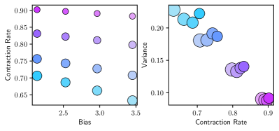
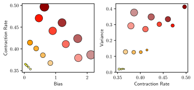
Figure 3: A toy example in the random MDP. In both figures, the color darkens with a larger $\tau$ ($\tau\in\{0.6,0.7,0.8,0.9\}$). The size of the spots is proportional to the relative scale of the third variable: (a) Change $n_{\rm max}$. From magenta to blue, $n_{\rm max}$ is set as $1,2,3,4$ in order. (b) Change the behavior polices $\mu$, where $\mu(s)=\text{softmax}(Q^{*}(s,\cdot)/\alpha)$. From light yellow to dark red, the $\alpha$ is set as $0.1,0.3,1,3$ in order.

4.2 Value-based Episodic Memory

In this part, we demonstrate that the memory-based planning effectively accelerates the convergence of the EVL. We first define the VEM operator as:

$$(\mathcal{T}_{\rm vem}V)(s)=\max_{1\leq n\leq n_{\rm max}}\{(\mathcal{T}^{\mu})^{n-1}\mathcal{T}_{\tau}^{\mu}V(s)\},$$ (9)

where $n_{\rm max}$ is the maximal rollout step for memory control. Then, we derive that multi-step estimation operator $\mathcal{T}_{\rm vem}$ does not change the fixed point and contraction property of $\mathcal{T}_{\tau}^{\mu}$:

Lemma 4.

Given $\tau\in(0,1)$ and $n_{\rm max}\in\mathbb{N}^{+}$, $\mathcal{T}_{\rm vem}$ is a $\gamma_{\tau}$-contraction. If $\tau>\frac{1}{2}$, $\mathcal{T}_{\rm vem}$ has the same fixed point as $\mathcal{T}_{\tau}^{\mu}$.

Next, we derive that the contraction rate of $\mathcal{T}_{\rm vem}$ depends on the dataset quality. Further, we demonstrate that the convergence rate of $\mathcal{T}_{\rm vem}$ is quicker than $\mathcal{T}_{\tau}^{\mu}$ even the behavior policy $\mu$ is random:

Lemma 5.

When the current value estimates $V(s)$ are much lower than the value of behavior policy, $\mathcal{T}_{\rm vem}$ provides an optimistic update. Formally, we have

$$|\mathcal{T}_{\rm vem}V(s)-V_{\tau}^{*}(s)|\leq\gamma^{n^{*}(s)-1}\gamma_{\tau}\|V-V_{n^{*},\tau}^{\mu}\|_{\infty}+\|V_{n^{*},\tau}^{\mu}-V_{\tau}^{*}\|_{\infty},\forall s\in S,$$ (10)

where $n^{*}(s)=\operatorname*{arg\,max}_{0<n\leq n_{\rm max}}\{(\mathcal{T}^{\mu})^{n-1}\mathcal{T}_{\tau}^{\mu}V(s)\}$, $V_{n^{*},\tau}^{\mu}$ is the fixed point of $(\mathcal{T}^{\mu})^{n^{*}(s)-1}\mathcal{T}_{\tau}^{\mu}$ and it is the optimal rollout value starting from $s$.

This lemma demonstrates that $\mathcal{T}_{\rm vem}$ can provide an optimistic update for pessimistic value estimates. Specifically, the scale of the update depends on the quality of the datasets. If the behavior policy $\mu$ is expert, which means $V_{n^{*},\tau}^{\mu}$ is close to $V_{\tau}^{*}$. Then, following the lemma, the contraction rate will be near to $\gamma^{n^{*}(s)-1}\gamma_{\tau}$. Moreover, if the initial value estimates are pessimistic (e.g., the initialized value function with zeros), we will have $n^{*}(s)\approx n_{\rm max}$, indicating that the value update will be extremely fast towards a lower bound of $V_{\tau}^{*}$. On the contrary, if $\mu$ is random, we have $n^{*}(s)\approx 1$ and the value update will be slow towards $V_{\tau}^{*}$.

Remark 2.

By choosing a suitable $n_{\rm max}$, we can achieve the trade-off between the contraction rate and the estimation variance, i.e., a larger $n_{\rm max}$ yields a fast update towards a lower bound of fixed point and tolerable variances empirically. Meanwhile, the choice of $n_{\rm max}$ does not introduce additional bias, and the fixed point bias is totally controlled by $\tau$.

4.3 Toy Example

We design a toy example in the random deterministic MDP to empirically demonstrate the above analysis. Following (Rowland et al., 2020), we adopt three indicators, including update variance, fixed-point bias, and contraction rate, which is shown in Figure 3. Specifically, the contraction rate is $\sup_{V\neq V^{\prime}}\|\mathcal{T}_{\rm vem}V-\mathcal{T}_{\rm vem}V^{\prime}\|_{\infty}/\|V-V^{\prime}\|_{\infty}$, the bias is $\|V_{\rm vem}^{*}-V^{*}\|_{\infty}$ and the variance is $\mathbb{E}\left[\|\hat{\mathcal{T}}V-\mathcal{T}_{\rm vem}V\|_{2}^{2}\right]^{\frac{1}{2}}$, where $\hat{\mathcal{T}}_{\rm vem}$ is the stochastic approximation of $\mathcal{T}_{\rm vem}$ and $V_{\rm vem}^{*}$ is the fixed pointed of $\mathcal{T}_{\rm vem}$. First, the experimental results in Figure 3(a) demonstrate that the relationship of $n$-step estimation and $\tau$. Formally, the contraction rate decreases as $n$ becomes larger, and the fixed-point bias increases as $\tau$ becomes smaller, which are consistent with Lemma 1 and Lemma 2. Figure 3(a) also shows that the variance is positively correlated with $n$. Second, the experimental results in Figure 3(b) demonstrate that the relationship of dataset quality and $\tau$. The higher dataset quality corresponds to the lower contraction rate and variance, which is consistent with Lemma 5.

5 Related Work

Offline Reinforcement Learning.

Offline RL methods (Kumar et al., 2019; Siegel et al., 2020; Argenson & Dulac-Arnold, 2020; Wu et al., 2021; Dadashi et al., 2021; Kostrikov et al., 2021; Jin et al., 2021; Rashidinejad et al., 2021) can be roughly divided into policy constraint, pessimistic value estimation, and model-based methods. Policy constraint methods aim to keep the policy to be close to the behavior under a probabilistic distance (Fujimoto et al., 2019; Peng et al., 2019; Nair et al., 2020). Pessimistic value estimation methods like CQL (Kumar et al., 2020) enforces a regularization constraint on the critic loss to penalize overgeneralization. Model-based methods attempt to learn a model from offline data, with minimal modification to the policy learning  (Kidambi et al., 2020; Yu et al., 2020; Janner et al., 2019). However, these methods have to introduce additional behavioral policy models, dynamics models, or regularization terms (Zhang et al., 2020b; a; Lee et al., 2021). Another line of methods uses empirical return as the signal for policy learning, which confines learning within the dataset but leads to limited performance (Levine et al., 2020; Geist et al., 2019; Wang et al., 2021).

Episodic Control.

Episodic control aims to store good past experiences in a non-parametric memory and rapidly latch into past successful policies when encountering similar states instead of waiting for many optimization steps (Blundell et al., 2016).  Pritzel et al. (2017) and Lin et al. (2018) introduce a parametric memory, which enables better generalization through neural networks. Our work is closely related to recent advances in  Hu et al. (2021), which adopts an implicit planning scheme to enable episodic memory updates in continuous domains. However, our method conducts planning with expectile $V$-values to avoid overgeneralization on actions out of dataset support.

6 Experiments

In our experiments, we aim to answer the following questions: 1) How does our method performe compared to state-of-the-art offline RL algorithms on the D4RL benchmark dataset? 2) How does implicit planning affect the performance on sparse reward tasks? 3) Can expectile $V$-Learning effectively reduces the extrapolation error compared with other offline methods? 4) How does the critical parameter $\tau$ affect the performance of our method?

(a) Large

(b) Medium

(c) Umaze

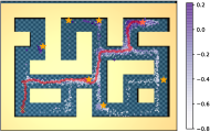
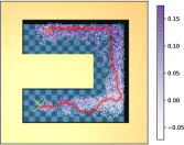
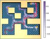
Figure 4: Visualization of the value estimation in various AntMaze tasks. Darker colors correspond to the higher value estimation. Each map has several terminals (golden stars) and one of which is reached by the agent (the light red star). The red line is the trajectory of the ant.

6.1 Evaluation environments

We ran VEM on AntMaze, Adroit, and MuJoCo environments to evaluate its performance on various types of tasks. Precisely, the AntMaze navigation tasks control an 8-DoF quadruped robot to reach a specific or randomly sampled goal in three types of maps. The reward in the AntMaze domain is highly sparse. The Adroit domain involves controlling a 24-DoF simulated hand tasked with hammering a nail, opening a door, twirling a pen, or picking up and moving a ball. On the adroit tasks, these datasets are the following, “human”: transitions collected by a human operator, “cloned”: transitions collected by a policy trained with behavioral cloning interacting in the environment + initial demonstrations, “expert”: transitions collected by a fine-tuned RL policy interacting in the environment. As for the MuJoCo tasks, the datasets are “random”: transitions collected by a random policy,“medium”: transitions collected by a policy with suboptimal performance. The complete implementation details are presented in Appendix C.

6.2 Performance on D4RL tasks

As shown in Table 1, VEM achieves state-of-the-art performance on most AntMaze tasks and has a significant improvement over other methods on most Adroit tasks. VEM also achieves good performances in MuJoCo domains. We find that VEM has low value estimation errors in all tasks, which promotes its superior performance. However, as a similar training framework, BAIL only has reasonable performances on simple offline tasks, such as MuJoCo. Please refer to Appendix D.2 for the complete training curves and value estimation error on D4RL.

To further analyze the superior performance of VEM in the sparse reward tasks, we visualize the learned value estimation in AntMaze tasks, which is shown in Figure 4. Experimental results show that VEM has the higher value estimates on the critical place of the map (e.g., corners) since various trajectories in the datasets are connected. The accurate value estimation leads to its success on complex sparse reward tasks.

Dataset Type	Environments	VEM(Ours)	BAIL	BCQ	CQL	AWR
fixed	antmaze-umaze	87.5$\pm$1.1	62.5 $\pm$ 2.3	78.9	74.0	56.0
play	antmaze-medium	78.0$\pm$3.1	40.0 $\pm$ 15.0	0.0	61.2	0.0
play	antmaze-large	57.0$\pm$5.0	23.0$\pm$5.0	6.7	11.8	0.0
diverse	antmaze-umaze	78.0 $\pm$ 1.1	75.0$\pm$1.0	55.0	84.0	70.3
diverse	antmaze-medium	77.0$\pm$2.2	50.0$\pm$10.0	0.0	53.7	0.0
diverse	antmaze-large	58.0 $\pm$ 2.1	30.0$\pm$5.0	2.2	14.9	0.0
human	adroit-door	11.2$\pm$4.2	0.0$\pm$0.1	-0.0	9.1	0.4
human	adroit-hammer	3.6$\pm$1.0	0.0$\pm$0.1	0.5	2.1	1.2
human	adroit-relocate	1.3$\pm$0.2	0.0$\pm$0.1	0.5	2.1	-0.0
human	adroit-pen	65.0$\pm$2.1	32.5$\pm$1.5	68.9	55.8	12.3
cloned	adroit-door	3.6$\pm$0.3	0.0$\pm$0.1	0.0	3.5	0.0
cloned	adroit-hammer	2.7$\pm$1.5	0.1$\pm$0.1	0.4	5.7	0.4
cloned	adroit-pen	48.7$\pm$3.2	46.5$\pm$3.5	44.0	40.3	28.0
expert	adroit-door	105.5$\pm$0.2	104.7$\pm$0.3	99.0	-	102.9
expert	adroit-hammer	128.3$\pm$1.1	123.5$\pm$3.1	114.9	-	39.0
expert	adroit-relocate	109.8$\pm$0.2	94.4$\pm$2.7	41.6	-	91.5
expert	adroit-pen	111.7$\pm$2.6	126.7$\pm$0.3	114.9	-	111.0
random	mujoco-walker2d	6.2$\pm$4.7	3.9$\pm$2.5	4.9	7.0	1.5
random	mujoco-hopper	11.1$\pm$1.0	9.8$\pm$0.1	10.6	10.8	10.2
random	mujoco-halfcheetah	16.4$\pm$3.6	0.0$\pm$0.1	2.2	35.4	2.5
medium	mujoco-walker2d	74.0$\pm$1.2	73.0$\pm$1.0	53.1	79.2	17.4
medium	mujoco-hopper	56.6$\pm$2.3	58.2$\pm$1.0	54.5	58.0	35.9
medium	mujoco-halfcheetah	47.4$\pm$0.2	42.6$\pm$1.2	40.7	44.4	37.4

Table 1: Performance of VEM with four offline RL baselines on the AntMaze, Adroit, and MuJoCo domains with the normalized score metric proposed by D4RL benchmark, averaged over three random seeds with $\pm$ standard deviation. Scores range from 0 to 100, where 0 corresponds to a random policy performance, and 100 indicates an expert. We use the results in Fu et al. (2020) for AWR and BCQ, and use the results in Kumar et al. (2020) for CQL. The results of BAIL come from our implementation according to the official code  (https://github.com/lanyavik/BAIL).

6.3 Analysis of Value Estimation

As both Expectile $V$-Learning (EVL) and Batch Constrained $Q$-Learning (BCQ) (Fujimoto et al., 2019) aim to avoid using the unseen state-action pairs to eliminate the extrapolation error, we replace EVL in VEM with BCQ (named BCQ-EM) to evaluate the effectiveness of the EVL module. The experimental results in Figure 5 indicate that the performance of BCQ-EM is mediocre, and BCQ reaches performance significantly below VEM. We observe a strong correlation between the training instability and the explosion of the value estimation. This result should not come as a surprise since the Adroit tasks have a larger action space compared with MuJoCo domains and narrow human demonstrations. Therefore, the generative model in BCQ cannot guarantees completely the unseen actions are avoided. In contrast, VEM avoids fundamentally unseen actions by keeping the learning procedure within the support of an offline dataset, indicating the necessity of the EVL module. Please refer to Appendix C for the implementation details.

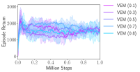
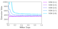
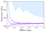
We evaluate $\tau\in\{0.1,0.2,...,0.9\}$ to investigate the effect of the critical hyper-parameter in EVL, which is shown in Figure 8 in Appendix D.1. The experimental results demonstrate that the estimated value increases with a larger $\tau$, which is consistent with the analysis in Section 4.1. Moreover, we observe that $\tau$ is set at a low value in some complex high-dimensional robotic tasks or narrow human demonstrations, such as Adroit-cloned/human, to get the conservative value estimates. However, if $\tau$ is set too high (e.g., $\tau=0.9$ in the pen-human task), the estimated value will explode and poor performance. This is as expected since the over-large $\tau$ leads to the overestimation error caused by neural networks. The experimental results demonstrate that we can balance behavior cloning and optimal value learning by choosing $\tau$ in terms of different tasks.

(a) door-human

(b) hammer-human

(c) relocate-human

(d) pen-human

(e) door-human

(f) hammer-human

(g) relocate-human

(h) pen-human

Figure 5: The comparison between VEM, BCQ-EM and BCQ on Adroit-human tasks. The results in the upper row are the performance. The results in the bottom row are the estimation error, where the unit is $10^{13}$.

(a) medium-play

(b) medium-diverse

(c) large-play

(d) large-diverse

Figure 6: The comparison between episodic memory and $n$-step value estimation on AntMaze tasks.

6.4 Ablations

Episodic Memory Module.

Our first study aims to answer the impact of memory-based planning on performance. We replace the episodic memory module in VEM with standard $n$-step value estimation (named VEM-1step or VEM-nstep). The experimental results in Figure 6 indicate that implicit planning along offline trajectories effectively accelerates the convergence of EVL.

Expectile Loss.

In addition to the Expectile loss, we explored other forms of loss. Formally, we compare the Expectile loss and quantile loss, a popular form in Distributional RL algorithms (Dabney et al., 2018), which is shown in Figure 7 in Appendix D.1. The experimental results indicate that the Expectile loss is better since it is more stable when dealing with extreme values.

7 Conclusion

In this paper, we propose a novel offline RL method, VEM, based on a new $V$-learning algorithm, EVL. EVL naturally avoids actions outside the dataset and provides a smooth tradeoff between generalization and conversation for offline learning. Further, VEM enables effective implicit planning along offline trajectories to accelerate the convergence of EVL and achieve better advantage estimation. Unlike most existing offline RL methods, we keep the learning procedure totally within the dataset’s support without any auxiliary modular, such as environment model or behavior policy. The experimental results demonstrate that VEM achieves superior performance in most D4RL tasks and learns the accurate values to guide policy learning, especially in sparse reward tasks. We hope that VEM will inspire more works on offline RL and promote practical RL methods in the future.

8 Reproducibility

To ensure our work is reproducible, we provide our code in the supplementary materials. In the future, we will publish all source code on Github. The detailed implementation of our algorithm is presented as follows. The value network is trained according to Equation 4. The actor-network is trained according to Equation 7. The hyper-parameters and network structure used in VEM are shown in Appendix C.3. All experiments are run on the standard offline tasks, D4RL (https://github.com/rail-berkeley/d4rl/tree/master/d4rl).

Appendix A Algorithm

A.1 Value-based Episodic Memory Control

Algorithm 1 Value-based Episodic Memory Control

  Initialize critic networks $V_{\theta_{1}},V_{\theta_{2}}$ and actor network $\pi_{\phi}$ with random parameters $\theta_{1},\theta_{2},\phi$

  Initialize target networks $\theta_{1}^{\prime}\leftarrow\theta_{1},\theta_{2}^{\prime}\leftarrow\theta_{2}$

  Initialize episodic memory $\mathcal{M}$

  for $t=1$ to $T$ do

     for $i\in\{1,2\}$ do

        Sample $N$ transitions $\left(s_{t},a_{t},r_{t},s_{t},R_{t}^{(i)}\right)$ from $\mathcal{M}$

        Update $\theta_{i}\leftarrow\text{min}_{\theta_{i}}N^{-1}\sum\left(R_{t}^{(i)}-V_{\theta_{i}}(s_{t})\right)^{2}$

        Update $\phi\leftarrow\text{max}_{\phi}N^{-1}\sum\nabla\log\pi_{\phi}(a_{t}|s_{t})\cdot f\left(\text{min}_{i}R_{t}^{(i)}-\text{mean}_{i}V_{\theta_{i}}(s_{t})\right)$

     end for

     if $t\text{ mod }u$ then

        $\theta_{i}^{\prime}\leftarrow\kappa\theta_{i}+(1-\kappa)\theta_{i}^{\prime}$

        Update Memory

     end if

  end for

Algorithm 2 Update Memory

  for trajectories $\tau$ in buffer $\mathcal{M}$ do

     for $s_{t},a_{t},r_{t},s_{t+1}$ in $\text{reversed}(\tau)$ do

        for $i\in\{1,2\}$ do

           Compute $R_{t}^{(i)}$ with Equation 6 and save into buffer $\mathcal{M}$

        end for

     end for

  end for

Appendix B Theoretical Analysis

B.1 Complete derivation.

The expectile regression loss (Rowland et al., 2019) is defined as

$$\operatorname{ER}(q;\varrho,\tau)=\mathbb{E}_{Z\sim\varrho}\left[\left[\tau\mathbb{I}_{Z>q}+(1-\tau)\mathbb{I}_{Z\leq q}\right](Z-q)^{2}\right],$$ (11)

where $\varrho$ is the target distribution and the minimiser of this loss is called the $\tau$-expectile of $\varrho$. the corresponding loss in reinforcement learning is

$$\mathcal{J}_{V}(\theta) =\mathbb{E}_{\mu}\left[\tau(r(s,a)+\gamma V_{\theta^{\prime}}(s^{\prime})-V_{\theta}(s))_{+}^{2}+(1-\tau)(r(s,a)+\gamma V_{\theta^{\prime}}(s^{\prime})-V_{\theta}(s))_{-}^{2}\right]$$ (12)

$$=\mathbb{E}_{\mu}\left[\tau(y-V_{\theta}(s))_{+}^{2}+(1-\tau)(y-V_{\theta}(s))_{-}^{2}\right].$$

Then, taking the gradient of the value objective:

$$\nabla\mathcal{J}_{V}(\theta) =\sum\mu(a\mid s)\left[-2\tau(y-V_{\theta})_{+}\mathbb{I}(y-V_{\theta})-2(1-\tau)(y-V_{\theta})_{+}\mathbb{I}(y-V_{\theta})\right]$$ (13)

$$=\sum\mu(a\mid s)\left[-2\tau(y-V_{\theta})_{+}-2(1-\tau)(y-V_{\theta})_{+}\right]$$

$$=\sum\mu(a\mid s)\left[-2\tau(\delta)_{+}-2(1-\tau)(\delta)_{+}\right].$$

Therefore,

$$\hat{V}(s) =V_{\theta}(s)-\alpha\nabla\mathcal{J}_{V}(\theta)$$ (14)

$$=V_{\theta}(s)+2\alpha\mathbb{E}_{a\sim\mu}\left[\tau[\delta(s,a)]_{+}+(1-\tau)[\delta(s,a)]_{-}\right]$$

B.2 Proof of Lemma 1

Lemma 1.

For any $\tau\in[0,1)$, $\mathcal{T}_{\tau}^{\mu}$ is a $\gamma_{\tau}$-contraction, where $\gamma_{\tau}=1-2\alpha(1-\gamma)\min\{\tau,1-\tau\}$.

Proof.

Note that $\mathcal{T}_{1/2}^{\mu}$ is the standard policy evaluation Bellman operator for $\mu$, whose fixed point is $V^{\mu}$. We see that for any $V_{1},V_{2}$,

$$\mathcal{T}_{1/2}^{\mu}V_{1}(s)-\mathcal{T}_{1/2}^{\mu}V_{2}(s)$$ (15)

$$=V_{1}(s)+\alpha\mathbb{E}_{a\sim\mu}[\delta_{1}(s,a)]-(V_{2}(s)+\alpha\mathbb{E}_{a\sim\mu}[\delta_{2}(s,a)])$$

$$=(1-\alpha)(V_{1}(s)-V_{2}(s))+\alpha\mathbb{E}_{a\sim\mu}[r(s,a)+\gamma V_{1}(s^{\prime})-r(s,a)-\gamma V_{2}(s^{\prime})]$$

$$\leq(1-\alpha)\|V_{1}-V_{2}\|_{\infty}+\alpha\gamma\|V_{1}-V_{2}\|_{\infty}$$

$$=(1-\alpha(1-\gamma))\|V_{1}-V_{2}\|_{\infty}.$$

We introduce two more operators to simplify the analysis:

$$\mathcal{T}_{+}^{\mu}V(s)=V(s)+\mathbb{E}_{a\sim\mu}[\delta(s,a)]_{+},$$ (16)

$$\mathcal{T}_{-}^{\mu}V(s)=V(s)+\mathbb{E}_{a\sim\mu}[\delta(s,a)]_{-}.$$

Next we show that both operators are non-expansion (e.g., $\|\mathcal{T}_{+}^{\mu}V_{1}-\mathcal{T}_{+}^{\mu}V_{2}\|_{\infty}\leq\|V_{1}-V_{2}\|_{\infty}$). For any $V_{1},V_{2}$, we have

$$\mathcal{T}_{+}^{\mu}V_{1}(s)-\mathcal{T}_{+}^{\mu}V_{2}(s) =V_{1}(s)-V_{2}(s)+\mathbb{E}_{a\sim\mu}[[\delta_{1}(s,a)]_{+}-[\delta_{2}(s,a)]_{+}]$$ (17)

$$=\mathbb{E}_{a\sim\mu}[[\delta_{1}(s,a)]_{+}+V_{1}(s)-([\delta_{2}(s,a)]_{+}+V_{2}(s))].$$

The relationship between $[\delta_{1}(s,a)]_{+}+V_{1}(s)$ and $[\delta_{2}(s,a)]_{+}+V_{2}(s)$ exists in four cases, which are

• $\delta_{1}\geq 0,\delta_{2}\geq 0$, then $[\delta_{1}(s,a)]_{+}+V_{1}(s)-([\delta_{2}(s,a)]_{+}+V_{2}(s))=\gamma(V_{1}(s^{\prime})-V_{2}(s^{\prime}))$.

• $\delta_{1}<0,\delta_{2}<0$, then $[\delta_{1}(s,a)]_{+}+V_{1}(s)-([\delta_{2}(s,a)]_{+}+V_{2}(s))=V_{1}(s)-V_{2}(s)$.

• $\delta_{1}\geq 0,\delta_{2}<0$, then

  $$[\delta_{1}(s,a)]_{+}+V_{1}(s)-([\delta_{2}(s,a)]_{+}+V_{2}(s))$$ (18)

  $$=(r(s,a)+\gamma V_{1}(s^{\prime}))-V_{2}(s)$$

  $$<(r(s,a)+\gamma V_{1}(s^{\prime}))-(r(s,a)+\gamma V_{2}(s^{\prime}))$$

  $$=\gamma(V_{1}(s^{\prime})-V_{2}(s^{\prime})),$$

  where the inequality comes from $r(s,a)+\gamma V_{2}(s^{\prime})<V_{2}(s)$.

• $\delta_{1}<0,\delta_{2}\geq 0$, then

  $$[\delta_{1}(s,a)]_{+}+V_{1}(s)-([\delta_{2}(s,a)]_{+}+V_{2}(s))$$ (19)

  $$=V_{1}(s)-(r(s,a)+\gamma V_{2}(s^{\prime}))$$

  $$\leq V_{1}(s)-V_{2}(s),$$

  where the inequality comes from $r(s,a)+\gamma V_{2}(s^{\prime})\geq V_{2}(s)$.

Therefore, we have $\mathcal{T}_{+}^{\mu}V_{1}(s)-\mathcal{T}_{+}^{\mu}V_{2}(s)\leq\|V_{1}-V_{2}\|_{\infty}$. With the $\mathcal{T}_{+}^{\mu},\mathcal{T}_{-}^{\mu}$, we rewrite $\mathcal{T}_{\tau}^{\mu}$ as

$$\mathcal{T}_{\tau}^{\mu}V(s) =V(s)+2\alpha\mathbb{E}_{a\sim\mu}[\tau[\delta(s,a)]_{+}+(1-\tau)[\delta(s,a)]_{-}]$$ (20)

$$=(1-2\alpha)V(s)+2\alpha\tau(V(s)+\mathbb{E}_{a\sim\mu}[\delta(s,a)]_{+})+2\alpha(1-\tau)(V(s)+\mathbb{E}_{a\sim\mu}[\delta(s,a)]_{-})$$

$$=(1-2\alpha)V(s)+2\alpha\tau\mathcal{T}_{+}^{\mu}V(s)+2\alpha(1-\tau)\mathcal{T}_{-}^{\mu}V(s).$$

And

$$\mathcal{T}_{1/2}^{\mu}V(s) =V(s)+\alpha\mathbb{E}_{a\sim\mu}[\delta(s,a)]$$ (21)

$$=V(s)+\alpha(\mathcal{T}_{+}^{\mu}V(s)+\mathcal{T}_{-}^{\mu}V(s)-2V(s))$$

$$=(1-2\alpha)V(s)+\alpha(\mathcal{T}_{+}^{\mu}V(s)+\mathcal{T}_{-}^{\mu}V(s)).$$

We first focus on $\tau<\frac{1}{2}$. For any $V_{1},V_{2}$, we have

$$\mathcal{T}_{\tau}^{\mu}V_{1}(s)-\mathcal{T}_{\tau}^{\mu}V_{2}(s)$$ (22)

$$=(1-2\alpha)(V_{1}(s)-V_{2}(s))+2\alpha\tau(\mathcal{T}_{+}^{\mu}V_{1}(s)-\mathcal{T}_{+}^{\mu}V_{2}(s))+2\alpha(1-\tau)(\mathcal{T}_{-}^{\mu}V_{1}(s)-\mathcal{T}_{-}^{\mu}V_{2}(s))$$

$$=(1-2\alpha-2\tau(1-2\alpha))(V_{1}(s)-V_{2}(s))+2\tau\left(\mathcal{T}^{\mu}_{1/2}V_{1}(s)-\mathcal{T}^{\mu}_{1/2}V_{2}(s)\right)+$$

$$\qquad\qquad\qquad\qquad\qquad\qquad\qquad\qquad\qquad\qquad 2\alpha(1-2\tau)\left(\mathcal{T}^{\mu}_{-}V_{1}(s)-\mathcal{T}^{\mu}_{-}V_{2}(s)\right)$$

$$\leq(1-2\alpha-2\tau(1-2\alpha))\|V_{1}-V_{2}\|_{\infty}+2\tau(1-\alpha(1-\gamma))\|V_{1}-V_{2}\|_{\infty}+2\alpha(1-2\tau)\|V_{1}-V_{2}\|_{\infty}$$

$$=(1-2\alpha\tau(1-\gamma))\|V_{1}-V_{2}\|_{\infty}$$

Similarly, when $\tau>1/2$, we have $\mathcal{T}_{\tau}^{\mu}V_{1}(s)-\mathcal{T}_{\tau}^{\mu}V_{2}(s)\leq(1-2\alpha(1-\tau)(1-\gamma))\|V_{1}-V_{2}\|_{\infty}$. ∎

B.3 Proof of Lemma 2

Lemma 2.

For any $\tau,\tau^{\prime}\in(0,1)$, if $\tau^{\prime}\geq\tau$, we have $\mathcal{T}_{\tau^{\prime}}^{\mu}\geq\mathcal{T}_{\tau}^{\mu},\forall s\in S$.

Proof.

Based on Equation 20, we have

$$\mathcal{T}_{\tau^{\prime}}^{\mu}V(s)-\mathcal{T}_{\tau}^{\mu}V(s)$$ (23)

$$=(1-2\alpha)V(s)+2\alpha\tau^{\prime}\mathcal{T}_{+}^{\mu}V(s)+2\alpha(1-\tau^{\prime})\mathcal{T}_{-}^{\mu}V(s)$$

$$\qquad\qquad\qquad-((1-2\alpha)V(s)+2\alpha\tau\mathcal{T}^{\mu}_{+}V(s)+2\alpha(1-\tau)\mathcal{T}_{-}^{\mu}V(s))$$

$$=2\alpha(\tau^{\prime}-\tau)(\mathcal{T}^{\mu}_{+}V(s)-\mathcal{T}^{\mu}_{-}V(s))$$

$$=2\alpha(\tau^{\prime}-\tau)\mathbb{E}_{a\sim\mu}[[\delta(s,a)]_{+}-[\delta(s,a)]_{-}]\geq 0.$$

∎

B.4 Proof of Lemma 3

Lemma 3.

Let $V^{*}$ denote the fixed point of Bellman optimality operator $\mathcal{T}^{*}$. In the deterministic MDP, we have $\lim_{\tau\to 1}V_{\tau}^{*}=V^{*}$.

Proof.

We first show that $V^{*}$ is also a fixed point for $\mathcal{T}_{+}^{\mu}$. Based on the definition of $\mathcal{T}^{*}$, we have $V^{*}(s)=\max_{a}[r(s,a)+\gamma V^{*}(s^{\prime})]$, which infers that $\delta(s,a)\leq 0$, $\forall s\in S,a\in A$. Thus, we have $\mathcal{T}_{+}^{\mu}V^{*}(s)=V^{*}(s)+\mathbb{E}_{a\sim\mu}[\delta(s,a)]_{+}=V^{*}(s)$. By setting $(1-\tau)\to 0$, we eliminate the effect of $\mathcal{T}_{-}^{\mu}$. Further by the contractive property of $\mathcal{T}_{\tau}^{\mu}$, we obtain the uniqueness of $V_{\tau}^{*}$. The proof is completed. ∎

B.5 Proof of Lemma 4

Lemma 4.

Given $\tau\in(0,1)$ and $T\in\mathbb{N}^{+}$, $\mathcal{T}_{\rm vem}$ is a $\gamma_{\tau}$-contraction. If $\tau>\frac{1}{2}$, $\mathcal{T}_{\rm vem}$ has the same fixed point as $\mathcal{T}_{\tau}^{\mu}$.

Proof.

We prove the contraction first. For any $V_{1},V_{2}$, we have

$$\mathcal{T}_{\rm vem}V_{1}(s)-\mathcal{T}_{\rm vem}V_{2}(s) =\max_{1\leq n\leq n_{\rm max}}\{(\mathcal{T}^{\mu})^{n-1}\mathcal{T}_{\tau}^{\mu}V_{1}(s)\}-\max_{1\leq n\leq T}\{(\mathcal{T}^{\mu})^{n-1}\mathcal{T}_{\tau}^{\mu}V_{2}(s)\}$$ (24)

$$\leq\max_{1\leq n\leq n_{\rm max}}|(\mathcal{T}^{\mu})^{n-1}\mathcal{T}_{\tau}^{\mu}V_{1}(s)-(\mathcal{T}^{\mu})^{n-1}\mathcal{T}_{\tau}^{\mu}V_{2}(s)|$$

$$\leq\max_{1\leq n\leq n_{\rm max}}\gamma^{n-1}\gamma_{\tau}\|V_{1}-V_{2}\|_{\infty}$$

$$\leq\gamma_{\tau}\|V_{1}-V_{2}\|_{\infty}.$$

Next we show that $V_{\tau}^{*}$, the fixed point of $\mathcal{T}_{\tau}^{\mu}$, is also the fixed point of $\mathcal{T}_{\rm vem}$ when $\tau>\frac{1}{2}$. By definition, we have $V_{\tau}^{*}=\mathcal{T}_{\tau}^{\mu}V_{\tau}^{*}$. Following Lemma 2, we have $V_{\tau}^{*}=\mathcal{T}_{\tau}^{\mu}V_{\tau}^{*}\geq\mathcal{T}_{1/2}^{\mu}V_{\tau}^{*}=\mathcal{T}^{\mu}V_{\tau}^{*}$. Repeatedly applying $\mathcal{T}^{\mu}$ and using its monotonicity, we have $\mathcal{T}^{\mu}V_{\tau}^{*}\geq(\mathcal{T}^{\mu})^{n-1}V_{\tau}^{*},1\leq n\leq n_{\rm max}$. Thus, we have $\mathcal{T}_{\rm vem}V_{\tau}^{*}(s)=\max_{1\leq n\leq T}\{(\mathcal{T}^{\mu})^{n-1}\mathcal{T}_{\tau}^{\mu}V_{\tau}^{*}(s)\}=V_{\tau}^{*}(s)$. ∎

B.6 Proof of Lemma 5

Lemma 5.

When the current value estimates $V(s)$ are much lower than the value of behavior policy, $\mathcal{T}_{\rm vem}$ provides an optimistic update. Formally, we have

$$|\mathcal{T}_{\rm vem}V(s)-V_{\tau}^{*}(s)|\leq\gamma^{n^{*}(s)-1}\gamma_{\tau}\|V-V_{n^{*},\tau}^{\mu}\|_{\infty}+\|V_{n^{*},\tau}^{\mu}-V_{\tau}^{*}\|_{\infty},\forall s\in S,$$ (25)

where $n^{*}(s)=\arg\max_{1\leq n\leq T}\{(\mathcal{T}^{\mu})^{n-1}\mathcal{T}_{\tau}^{\mu}V(s)\}$ and $V_{n^{*},\tau}^{\mu}$ is the fixed point of $(\mathcal{T}^{\mu})^{n^{*}(s)-1}\mathcal{T}_{\tau}^{\mu}$.

Proof.

The lemma is a direct result of the triangle inequality. We have

$$\mathcal{T}_{\rm vem}V(s)-V_{\tau}^{*}(s) =(\mathcal{T}^{\mu})^{n^{*}(s)-1}\mathcal{T}_{\tau}^{\mu}V(s)-V_{\tau}^{*}(s)$$ (26)

$$=(\mathcal{T}^{\mu})^{n^{*}(s)-1}\mathcal{T}_{\tau}^{\mu}V(s)-(\mathcal{T}^{\mu})^{n^{*}(s)-1}\mathcal{T}_{\tau}^{\mu}V_{n^{*},\tau}^{\mu}(s)+V_{n^{*},\tau}^{\mu}(s)-V_{\tau}^{*}(s)$$

$$\leq\gamma^{n^{*}(s)-1}\gamma_{\tau}\|V-V_{n^{*},\tau}^{\mu}\|_{\infty}+\|V_{n^{*},\tau}^{\mu}-V_{\tau}^{*}\|.$$

∎

B.7 Proof of Proposition 1

Proposition 1.

Let $V_{\tau}^{*}$ denote the fixed point of $\mathcal{T}_{\tau}^{\mu}$. For any $\tau,\tau^{\prime}\in(0,1)$, if $\tau^{\prime}\geq\tau$, we have $V_{\tau^{\prime}}^{*}(s)\geq V_{\tau}^{*}(s)$, $\forall s\in S$.

Proof.

With the Lemma 2, we have $\mathcal{T}_{\tau^{\prime}}^{\mu}V_{\tau}^{*}\geq\mathcal{T}_{\tau}^{\mu}V_{\tau}^{*}$. Since $V_{\tau}^{*}$ is the fixed point of $\mathcal{T}_{\tau}^{\mu}$, we have $\mathcal{T}_{\tau}^{\mu}V_{\tau}^{*}=V_{\tau}^{*}$. Putting the results together, we obtain $V_{\tau}^{*}=\mathcal{T}_{\tau}^{\mu}V_{\tau}^{*}\leq\mathcal{T}_{\tau^{\prime}}^{\mu}V_{\tau}^{*}$. Repeatedly applying $\mathcal{T}_{\tau^{\prime}}^{\mu}$ and using its monotonicity, we have $V_{\tau}^{*}\leq\mathcal{T}_{\tau^{\prime}}^{\mu}V_{\tau}^{*}\leq\left(\mathcal{T}_{\tau^{\prime}}^{\mu}\right)^{\infty}V_{\tau}^{*}=V_{\tau^{\prime}}^{*}$. ∎

Appendix C Detailed Implementation

C.1 Generalized Advantage-Weighted Learning

In practice, we adopt Leaky-ReLU or Softmax functions.

Leaky-ReLU:

$$\max_{\phi}J_{\pi}(\phi) =\mathbb{E}_{(s,a)\sim\mathcal{D}}\left[\log\pi_{\phi}(a\mid s)\cdot f\left(\hat{A}(s,a)\right)\right],$$ (27)

where $$f(\hat{A}(s,a))=\begin{cases}\hat{A}(s,a)\qquad\text{if}\quad\hat{A}(s,a)>0\\ \frac{\hat{A}(s,a)}{\alpha}\qquad\text{if}\quad\hat{A}(s,a)\leq 0\\ \end{cases}$$

Softmax:

$$\max_{\phi}J_{\pi}(\phi)=\mathbb{E}_{(s,a)\sim\mathcal{D}}\left[\log\pi_{\phi}(a\mid s)\cdot\frac{\exp(\frac{1}{\alpha}\hat{A}(s,a))}{\sum_{(s_{i},a_{i})\sim\text{Batch}}\exp(\frac{1}{\alpha}\hat{A}(s_{i},a_{i}))}\right].$$ (28)

C.2 BCQ-EM

The value network of BCQ-EM is trained by minimizing the following loss:

$$\min_{\theta}\mathcal{J}_{Q}(\theta) =\mathbb{E}_{(s_{t},a_{t},s_{t+1})\sim\mathcal{D}}\left[\left(R_{t}-Q_{\theta}(s_{t},a_{t})\right)^{2}\right]$$ (29)

$$R_{t} =\max_{0<n\leq n_{\rm max}}Q_{t,n},\quad Q_{t,n}=\begin{cases}r_{t}+\gamma Q_{t+1,n-1}(s_{t+1},\hat{a}_{t+1})&\text{if}\quad n>0,\\ Q(s_{t},\hat{a}_{t})&\text{if}\quad n=0,\end{cases}$$ (30)

where $\hat{a}_{t}$ corresponds to the perturbed actions, sampled from the generative model $G_{w}(s_{t})$.

The perturbation network of BCQ-EM is trained by minimizing the following loss:

$$\min_{\phi}\mathcal{J}_{\xi}(\phi)=-\mathbb{E}_{s\sim\mathcal{D}}\left[Q_{\theta}(s,a_{i}+\xi_{\phi}(s,a_{i},\Phi))\right],\quad\{a_{i}\sim G_{w}(s)\}_{i=1}^{n},$$ (31)

where $\xi_{\phi}(s,a_{i},\Phi)$ is a perturbation model, which outputs an adjustment to an action $a$ in the range $[-\Phi,\Phi]$. We adopt conditional variational auto-encoder to represent the generative model $G_{w}(s)$ and it is trained to match the state-action pairs sampled from $\mathcal{D}$ by minimizing the cross-entropy loss-function.

C.3 Hyper-Parameter and Network Structure

Table 2: Hyper-parameter Sheet

Hyper-Parameter	Value
Critic Learning Rate	1e-3
Actor Learning Rate	1e-3
Optimizer	Adam
Target Update Rate ($\kappa$)	0.005
Memory Update Period	100
Batch Size	128
Discount Factor	0.99
Gradient Steps per Update	200
Maximum Length $d$	Episode Length $T$

Table 3: Hyper-Parameter $\tau$ used in VEM across different tasks

AntMaze-fixed	umaze	medium	large
	0.4	0.3	0.3
AntMaze-diverse	umaze	medium	large
	0.3	0.4	0.1
Adroit-human	door	hammer	pen
	0.4	0.4	0.4
Adroit-cloned	door	hammer	pen
	0.2	0.3	0.1
Adroit-expert	door	hammer	pen
	0.3	0.3	0.3
MuJoCo-medium	walker2d	halfcheetah	hopper
	0.4	0.4	0.5
MuJoCo-random	walker2d	halfcheetah	hopper
	0.5	0.6	0.7

We use a fully connected neural network as a function approximation with 256 hidden units and ReLU as an activation function. The structure of the actor network is $[(\text{state dim},256),(256,256),(256,\text{action dim})]$. The structure of the value network is $[(\text{state dim},256),(256,256),(256,1)]$.

Appendix D Additional Experiments on D4RL

D.1 Ablation Study

(a) door-human

(b) hammer-human

(c) relocate-human

(d) pen-human

Figure 7: Comparison results between expectile loss and quantile loss on Adroit tasks. We respectively name our algorithm with expectile loss and quantile loss as VEM and VEM (abs).

(a) pen-human

(b) door-human

(c) hammer-human

(d) pen-human

(e) door-human

(f) hammer-human

Figure 8: The results of VEM ($\tau$) with various $\tau$ in Adroit tasks. The results in the upper row are the performance. The results in the bottom row are the estimation value.

D.2 Complete training curves and value estimation error

(a) umaze

(b) umaze-diverse

(c) medium-play

(d) medium-diverse

(e) large-play

(f) large-diverse

(g) door-human

(h) hammer-human

(i) relocate-human

(j) pen-human

(k) door-cloned

(l) hammer-cloned

(m) pen-cloned

(n) hopper-medium

(o) walker2d-medium

(p) halfcheetah-medium

(q) hopper-random

(r) walker2d-random

(s) halfcheetah-random

Figure 9: The training curves of VEM and BAIL on D4RL tasks.

(a) umaze

(b) umaze-diverse

(c) medium-play

(d) medium-diverse

(e) large-play

(f) large-diverse

(g) door-human

(h) hammer-human

(i) relocate-human

(j) pen-human

(k) door-cloned

(l) hammer-cloned

(m) pen-cloned

(n) hopper-medium

(o) walker2d-medium

(p) halfcheetah-medium

(q) hopper-random

(r) walker2d-random

(s) halfcheetah-random

Figure 10: The value estimation error of VEM on D4RL tasks. The estimation error refers to the average estimated state values minus the average returns.

References

• Argenson & Dulac-Arnold (2020) Arthur Argenson and Gabriel Dulac-Arnold. Model-based offline planning. arXiv preprint arXiv:2008.05556, 2020.
• Blundell et al. (2016) Charles Blundell, Benigno Uria, Alexander Pritzel, Yazhe Li, Avraham Ruderman, Joel Z Leibo, Jack Rae, Daan Wierstra, and Demis Hassabis. Model-free episodic control. arXiv preprint arXiv:1606.04460, 2016.
• Chen et al. (2020) Xinyue Chen, Zijian Zhou, Zheng Wang, Che Wang, Yanqiu Wu, and Keith Ross. BAIL: Best-action imitation learning for batch deep reinforcement learning. Advances in Neural Information Processing Systems, 33, 2020.
• Dabney et al. (2018) Will Dabney, Mark Rowland, Marc G Bellemare, and Rémi Munos. Distributional reinforcement learning with quantile regression. In Thirty-Second AAAI Conference on Artificial Intelligence, 2018.
• Dadashi et al. (2021) Robert Dadashi, Shideh Rezaeifar, Nino Vieillard, Léonard Hussenot, Olivier Pietquin, and Matthieu Geist. Offline reinforcement learning with pseudometric learning. arXiv preprint arXiv:2103.01948, 2021.
• Fu et al. (2020) Justin Fu, Aviral Kumar, Ofir Nachum, George Tucker, and Sergey Levine. D4RL: Datasets for deep data-driven reinforcement learning. arXiv preprint arXiv:2004.07219, 2020.
• Fujimoto et al. (2019) Scott Fujimoto, David Meger, and Doina Precup. Off-policy deep reinforcement learning without exploration. In International Conference on Machine Learning, pp. 2052–2062. PMLR, 2019.
• Geist et al. (2019) Matthieu Geist, Bruno Scherrer, and Olivier Pietquin. A theory of regularized markov decision processes. In International Conference on Machine Learning, pp. 2160–2169. PMLR, 2019.
• Ghasemipour et al. (2021) Seyed Kamyar Seyed Ghasemipour, Dale Schuurmans, and Shixiang Shane Gu. EMaQ: Expected-max Q-learning operator for simple yet effective offline and online RL. In International Conference on Machine Learning, pp. 3682–3691. PMLR, 2021.
• Hu et al. (2021) Hao Hu, Jianing Ye, Zhizhou Ren, Guangxiang Zhu, and Chongjie Zhang. Generalizable episodic memory for deep reinforcement learning. arXiv preprint arXiv:2103.06469, 2021.
• Janner et al. (2019) Michael Janner, Justin Fu, Marvin Zhang, and Sergey Levine. When to trust your model: Model-based policy optimization. Advances in Neural Information Processing Systems, 32:12519–12530, 2019.
• Jin et al. (2021) Ying Jin, Zhuoran Yang, and Zhaoran Wang. Is pessimism provably efficient for offline RL? In International Conference on Machine Learning, pp. 5084–5096. PMLR, 2021.
• Kidambi et al. (2020) Rahul Kidambi, Aravind Rajeswaran, Praneeth Netrapalli, and Thorsten Joachims. Morel: Model-based offline reinforcement learning. arXiv preprint arXiv:2005.05951, 2020.
• Kostrikov et al. (2021) Ilya Kostrikov, Rob Fergus, Jonathan Tompson, and Ofir Nachum. Offline reinforcement learning with fisher divergence critic regularization. In International Conference on Machine Learning, pp. 5774–5783. PMLR, 2021.
• Kumar et al. (2019) Aviral Kumar, Justin Fu, Matthew Soh, George Tucker, and Sergey Levine. Stabilizing off-policy Q-learning via bootstrapping error reduction. Advances in Neural Information Processing Systems, 32:11784–11794, 2019.
• Kumar et al. (2020) Aviral Kumar, Aurick Zhou, George Tucker, and Sergey Levine. Conservative Q-learning for offline reinforcement learning. arXiv preprint arXiv:2006.04779, 2020.
• Lee et al. (2021) Jongmin Lee, Wonseok Jeon, Byung-Jun Lee, Joelle Pineau, and Kee-Eung Kim. OptiDICE: Offline policy optimization via stationary distribution correction estimation. arXiv preprint arXiv:2106.10783, 2021.
• Levine et al. (2020) Sergey Levine, Aviral Kumar, George Tucker, and Justin Fu. Offline reinforcement learning: Tutorial, review, and perspectives on open problems. arXiv preprint arXiv:2005.01643, 2020.
• Lin et al. (2018) Zichuan Lin, Tianqi Zhao, Guangwen Yang, and Lintao Zhang. Episodic memory deep Q-networks. In Proceedings of the 27th International Joint Conference on Artificial Intelligence, pp.  2433–2439, 2018.
• Nair et al. (2020) Ashvin Nair, Murtaza Dalal, Abhishek Gupta, and Sergey Levine. Accelerating online reinforcement learning with offline datasets. arXiv preprint arXiv:2006.09359, 2020.
• Newey & Powell (1987) Whitney K Newey and James L Powell. Asymmetric least squares estimation and testing. Econometrica: Journal of the Econometric Society, pp. 819–847, 1987.
• Peng et al. (2019) Xue Bin Peng, Aviral Kumar, Grace Zhang, and Sergey Levine. Advantage-weighted regression: Simple and scalable off-policy reinforcement learning. arXiv preprint arXiv:1910.00177, 2019.
• Pritzel et al. (2017) Alexander Pritzel, Benigno Uria, Sriram Srinivasan, Adria Puigdomenech Badia, Oriol Vinyals, Demis Hassabis, Daan Wierstra, and Charles Blundell. Neural episodic control. In International Conference on Machine Learning, pp. 2827–2836. PMLR, 2017.
• Rashidinejad et al. (2021) Paria Rashidinejad, Banghua Zhu, Cong Ma, Jiantao Jiao, and Stuart Russell. Bridging offline reinforcement learning and imitation learning: A tale of pessimism. arXiv preprint arXiv:2103.12021, 2021.
• Rowland et al. (2019) Mark Rowland, Robert Dadashi, Saurabh Kumar, Rémi Munos, Marc G Bellemare, and Will Dabney. Statistics and samples in distributional reinforcement learning. In International Conference on Machine Learning, pp. 5528–5536. PMLR, 2019.
• Rowland et al. (2020) Mark Rowland, Will Dabney, and Rémi Munos. Adaptive trade-offs in off-policy learning. In International Conference on Artificial Intelligence and Statistics, pp.  34–44. PMLR, 2020.
• Siegel et al. (2020) Noah Y Siegel, Jost Tobias Springenberg, Felix Berkenkamp, Abbas Abdolmaleki, Michael Neunert, Thomas Lampe, Roland Hafner, Nicolas Heess, and Martin Riedmiller. Keep doing what worked: Behavioral modelling priors for offline reinforcement learning. arXiv preprint arXiv:2002.08396, 2020.
• Tang (2020) Yunhao Tang. Self-imitation learning via generalized lower bound Q-learning. Advances in Neural Information Processing Systems, 33, 2020.
• Wang et al. (2018) Qing Wang, Jiechao Xiong, Lei Han, Peng Sun, Han Liu, and Tong Zhang. Exponentially weighted imitation learning for batched historical data. Advances in Neural Information Processing Systems, 31:6288, 2018.
• Wang et al. (2021) Ruosong Wang, Yifan Wu, Ruslan Salakhutdinov, and Sham M Kakade. Instabilities of offline rl with pre-trained neural representation. arXiv preprint arXiv:2103.04947, 2021.
• Wu et al. (2021) Yue Wu, Shuangfei Zhai, Nitish Srivastava, Joshua Susskind, Jian Zhang, Ruslan Salakhutdinov, and Hanlin Goh. Uncertainty weighted Actor-Critic for offline reinforcement learning. arXiv preprint arXiv:2105.08140, 2021.
• Yang et al. (2021) Yiqin Yang, Xiaoteng Ma, Chenghao Li, Zewu Zheng, Qiyuan Zhang, Gao Huang, Jun Yang, and Qianchuan Zhao. Believe what you see: Implicit constraint approach for offline multi-agent reinforcement learning. arXiv preprint arXiv:2106.03400, 2021.
• Yu et al. (2020) Tianhe Yu, Garrett Thomas, Lantao Yu, Stefano Ermon, James Y Zou, Sergey Levine, Chelsea Finn, and Tengyu Ma. MOPO: Model-based offline policy optimization. Advances in Neural Information Processing Systems, 33:14129–14142, 2020.
• Zhang et al. (2020a) Ruiyi Zhang, Bo Dai, Lihong Li, and Dale Schuurmans. GenDICE: Generalized offline estimation of stationary values. arXiv preprint arXiv:2002.09072, 2020a.
• Zhang et al. (2020b) Shangtong Zhang, Bo Liu, and Shimon Whiteson. GradientDICE: Rethinking generalized offline estimation of stationary values. In International Conference on Machine Learning, pp. 11194–11203. PMLR, 2020b.