Computationally Efficient Quantum Expectation with Extended Bell Measurements

Ruho Kondo Affiliation: Toyota Central R&D Labs., Inc., 41-1, Yokomichi, Nagakute, Aichi 480-1192, Japan Email: r-kondo@mosk.tytlabs.co.jp    Yuki Sato Affiliation: Toyota Central R&D Labs., Inc., 41-1, Yokomichi, Nagakute, Aichi 480-1192, Japan    Satoshi Koide Affiliation: Toyota Central R&D Labs., Inc., 41-1, Yokomichi, Nagakute, Aichi 480-1192, Japan    Seiji Kajita Affiliation: Toyota Central R&D Labs., Inc., 41-1, Yokomichi, Nagakute, Aichi 480-1192, Japan    Hideki Takamatsu Affiliation: Toyota Motor Corporation, 1 Toyota-Cho, Toyota, Aichi 471-8571, Japan
Abstract

Evaluating an expectation value of an arbitrary observable A2n×2nA\in{\mathbb{C}}^{2^{n}\times 2^{n}} through naïve Pauli measurements requires a large number of terms to be evaluated. We approach this issue using a method based on Bell measurement, which we refer to as the extended Bell measurement method. This analytical method quickly assembles the 4n4^{n} matrix elements into at most 2n+12^{n+1} groups for simultaneous measurements in O(nd)O(nd) time, where dd is the number of non-zero elements of AA. The number of groups is particularly small when AA is a band matrix. When the bandwidth of AA is k=O(nc)k=O(n^{c}), the number of groups for simultaneous measurement reduces to O(nc+1)O(n^{c+1}). In addition, when non-zero elements densely fill the band, the variance is O((nc+1/2n)tr(A2))O((n^{c+1}/2^{n})\,{\rm tr}(A^{2})), which is small compared with the variances of existing methods. The proposed method requires a few additional gates for each measurement, namely one Hadamard gate, one phase gate and at most n1n-1 CNOT gates. Experimental results on an IBM-Q system show the computational efficiency and scalability of the proposed scheme, compared with existing state-of-the-art approaches. Code is available at https://github.com/ToyotaCRDL/extended-bell-measurements.

1 Introduction

Variational quantum algorithms (VQAs) [1, 2] have attracted attention in recent years because they are suitable for so-called Noisy Intermediate-Scale Quantum (NISQ) computers [3], which do not have a fault-tolerant mechanism and have only tens or hundreds of qubits. The VQA was first introduced in the field of chemistry but it has wide application, such as in solving linear systems [4, 5, 6, 7, 8], optimization [9, 10, 11], and machine learning [12, 13, 14, 15, 16, 17, 18]. In VQAs, the quantum state, |ψ\big|\psi\big>, is parametrized by learning parameters held on a classical computer, and is used to calculate the expectation value, ψ|A|ψ\big<\psi\big|A\big|\psi\big>, whose AA depends on the task. The desired quantum state is then obtained by minimizing the expectation value using a classical optimization algorithm.

The bottleneck of a VQA relates to the computational cost of calculating the expectation value [19]. A popular method of evaluating the expectation value is a Pauli measurement that writes AA in the Pauli basis; i.e., A=i=1𝒩ci𝐏iA=\sum^{\mathcal{N}}_{i=1}c_{i}{\bf P}_{i}, where 𝐏i{\bf P}_{i} is the tensor product of Pauli matrices and ci=Tr(A𝐏i)/2nc_{i}={\rm Tr}\big(A^{\dagger}{\bf P}_{i}\big)/2^{n} is the corresponding coefficient, with ()(\bullet)^{\dagger} indicating the Hermitian conjugate. The drawback of a naïve Pauli measurement is that it requires a large number of unique circuits to evaluate ψ|A|ψ=i=1𝒩ciψ|𝐏i|ψ\big<\psi\big|A\big|\psi\big>=\sum^{\mathcal{N}}_{i=1}c_{i}\big<\psi\big|{\bf P}_{i}\big|\psi\big> where 𝒩\mathcal{N} reaches 4n4^{n} when AA is a fully dense matrix.

Reducing the number of unique circuits for Pauli measurements is an interesting topic relating to the VQA [20, 21, 22, 23, 24, 25, 26]. Both qubit-wise commuting (QWC) [27, 28, 21] and general commuting (GC) [24] methods, and their variants [22, 23, 26], reduce the number of unique circuits on the basis that commutative operators can be simultaneously diagonalized with the same unitary; i.e., commutative Pauli bases are simultaneously measurable. This approach successfully reduces the number of unique circuits but its weakness is that finding the smallest groups for simultaneous measurements itself is an NP-hard problem. These methods approximate solutions that are unfortunately not optimal in general. In other words, a smaller number of unique circuits results in a longer calculation time, and a shorter calculation time results in a larger number of unique circuits.

Another problem is that the expression of general matrices in the Pauli basis is numerically inefficient. Suppose a sparse matrix AA that has a few non-zero elements. In the extreme case, for example, if there exists just one non-zero element in AA, then 2n2^{n} Pauli strings are required to represent AA. Despite the inefficiency of the Pauli basis, the sparse matrix is widely used in the domain of computer science. A typical application is the finite element method (FEM) [29] used for structural analysis, fluid dynamics, heat transfer, electromagnetic analysis and many other continuum mechanics. In the FEM, three dimensional real-space is discretized by a finite number of elements and the stiffness of the system is constructed by the nodal coordinates and properties of each element. The resulting global stiffness matrix, AA, in an appropriate node number ordering represents a band matrix because only the neighboring nodes in the elements can interact with each other. Then, solving Ax=bAx=b, where bb denotes the external inputs, gives the desired response xx. Solving Ax=bAx=b using VQAs has long been studied [4, 5, 6, 7, 8] but most of the VQAs limit the form of AA. For example, the assumption is that AA can be represented as the sum of a few weighted unitaries or weighted Pauli strings [4, 5, 6] or can be decomposed into a few measurable terms using the problem–specific conditions [7, 8]. Recently, an efficient expectation estimation method for a sparse Hamiltonian has been developed [30], but it remains unsuitable for the NISQ device because of its two-qubit entangling gate counts. Efficient expectation evaluations for the non-Pauli observables in terms of both the number of measurements and the circuit complexity are in great demand, such as for FEM applications, but the above issues have not yet been resolved.

A completely different approach that can be taken to reduce the computational cost for the expectation evaluation is to use the so-called classical shadow [31, 32, 33], which reduces the number of measurements for the Pauli observables. However, in the case of non-Pauli observables, this approach is not suitable for NISQ devices because it requires O(n2/log(n))O(n^{2}/\log(n)) two-qubit entangling gates as pointed out in the original literature [31].

In this paper, we propose an alternative method that we refer to as the extended Bell measurement (XBM). This method is based on not Pauli measurements but Bell measurements. The basic idea is inspired by Ref. [7], where the expectation value required to solve the Poisson equation was evaluated using Bell measurements. We generalize this method for an arbitrary expectation evaluation. In addition, we derive that the present method is closely related to the classical shadow with random Clifford measurements [31]. The XBM method has the following advantages over existing methods.

  1. 1.

    Fast grouping: The XBM method does not solve any difficult NP-hard problems, but it analytically groups the simultaneous measurements.

  2. 2.

    Small number of circuits: The method requires the number of unique circuits to be of the same order as the empirical number of an existing state-of-the-art Pauli measurement-based method, such as the GC method.

  3. 3.

    Fewer two-qubit entangling gates: The method takes at most n1n-1 CNOT gates for each measurement operator.

  4. 4.

    Tight upper bound of the variance when AA is the densely filled band matrix.

Concretely, when AA is a band matrix whose bandwidth is k=O(nc)k=O(n^{c}), the number of distinct measurement operators is O(nc+1)O(n^{c+1}). In addition, when the non-zero elements are densely filled in the band, the upper bound of the variance of the expectation evaluation is O((nc+1/2n)tr(A2))O((n^{c+1}/2^{n})\,{\rm tr}(A^{2})), which is smaller than that of the classical shadow [31].

Our algorithm is implemented with Qiskit [34] and its code is available at https://github.com/ToyotaCRDL/extended-bell-measurements. Additionally, real-device experiments are carried out using an IBM-Q system. The results show that the accuracy of the expectation evaluation is comparable to that of naïve Pauli measurements and QWC but the execution time is shorter than the execution times of the existing methods when AA is a band matrix.

The remainder of the paper is organized as follows: Section 2 describes the XBM method proposed in this paper. Section 3 presents algorithms of the XBM method and derives the computational complexity. Section 4 presents the experimental results. Section 5 concludes the paper.

2 Method

2.1 Two-qubit Example of Proposed Method

Before describing the general proposed method, we show an example with two-qubit. Let |φ4|\varphi\rangle\in{\mathbb{C}}^{4} be an arbitrary two-qubit quantum state. Consider the following expectation value:

φ|A|φ=φ|[A00A01A02A03A10A11A12A13A20A21A22A23A30A31A32A33]|φ\displaystyle{\langle\varphi|A|\varphi\rangle=\langle\varphi|\begin{bmatrix}A_{00}&A_{01}&A_{02}&A_{03}\\ A_{10}&A_{11}&A_{12}&A_{13}\\ A_{20}&A_{21}&A_{22}&A_{23}\\ A_{30}&A_{31}&A_{32}&A_{33}\\ \end{bmatrix}|\varphi\rangle}
=b=03c=03Abcφ|bc|φ.\displaystyle{=\sum^{3}_{b=0}\sum^{3}_{c=0}A_{bc}\langle\varphi|b\rangle\langle c|\varphi\rangle.}

The diagonal components of AA can be easily evaluated as

b=03Abbφ|bb|φ=b=03Abb|b|φ|2\displaystyle{\sum^{3}_{b=0}A_{bb}\langle\varphi|b\rangle\langle b|\varphi\rangle=\sum^{3}_{b=0}A_{bb}|\langle b|\varphi\rangle|^{2}}

where |b|φ|2|\langle b|\varphi\rangle|^{2} is the probability of obtaining a bit-string bb when measuring the quantum state |φ|\varphi\rangle in the computational basis. Meanwhile, evaluating the off-diagonal parts of AA is not trivial. Consider A12A_{12} for example. The expectation value of A12A_{12} can be rearranged as

φ|[000000A12000000000]|φ=φ|(A12|12|)|φ\displaystyle{\langle\varphi|\begin{bmatrix}0&0&0&0\\ 0&0&A_{12}&0\\ 0&0&0&0\\ 0&0&0&0\\ \end{bmatrix}|\varphi\rangle=\langle\varphi|\Big(A_{12}|1\rangle\langle 2|\Big)|\varphi\rangle}
=A12(Re(φ|12|φ)+iIm(φ|12|φ))\displaystyle{=A_{12}\Big({\rm Re}\big(\langle\varphi|1\rangle\langle 2|\varphi\rangle\big)+{\rm i}{\rm Im}\big(\langle\varphi|1\rangle\langle 2|\varphi\rangle\big)\Big)}

where Re(){\rm Re}(\bullet) and Im(){\rm Im}(\bullet) are the real and imaginary parts of ()(\bullet), respectively. The real part of φ|12|φ\langle\varphi|1\rangle\langle 2|\varphi\rangle is further rearranged as

Re(φ|12|φ)\displaystyle{{\rm Re}\big(\langle\varphi|1\rangle\langle 2|\varphi\rangle\big)}
=12(|01|+10|2|φ|2|01|10|2|φ|2)\displaystyle{=\frac{1}{2}\Bigg(\Bigg|\frac{\langle 01|+\langle 10|}{\sqrt{2}}|\varphi\rangle\Bigg|^{2}-\Bigg|\frac{\langle 01|-\langle 10|}{\sqrt{2}}|\varphi\rangle\Bigg|^{2}\Bigg)}

where |01=|1|01\rangle=|1\rangle and |10=|2|10\rangle=|2\rangle, respectively. The quantum states (|01±|10)/2(|01\rangle\pm|10\rangle)/\sqrt{2} can be prepared using the Hadamard gate and CNOT gate as

|01+|102=CNOT(1,0)H(1)|01\displaystyle{\frac{|01\rangle+|10\rangle}{\sqrt{2}}={\rm CNOT}(1,0){\rm H}(1)|01\rangle}
|01|102=CNOT(1,0)H(1)|11\displaystyle{\frac{|01\rangle-|10\rangle}{\sqrt{2}}={\rm CNOT}(1,0){\rm H}(1)|11\rangle}

where H(j){\rm H}(j) denotes the Hadamard gate acting on jjth qubit, and CNOT(j,k){\rm CNOT}(j,k) is the CNOT gate whose control and target qubits are jjth and kkth qubits, respectively. Here, the rightmost bit is 0th bit whereas the leftmost bit is (n1)(n-1)th bit. Using these preparation unitaries, Re(φ|12|φ){\rm Re}\big(\langle\varphi|1\rangle\langle 2|\varphi\rangle\big) is written as

Re(φ|12|φ)=12(|01|H(1)CNOT(1,0)|φ|2CLOSE\displaystyle{{\rm Re}\big(\langle\varphi|1\rangle\langle 2|\varphi\rangle\big)=\frac{1}{2}\Bigg(\Big|\langle 01|{\rm H}(1){\rm CNOT}(1,0)|\varphi\rangle\Big|^{2}}
OPEN|11|H(1)CNOT(1,0)|φ|2).\displaystyle{-\Big|\langle 11|{\rm H}(1){\rm CNOT}(1,0)|\varphi\rangle\Big|^{2}\Bigg).}

This value can be evaluated by the probabilities of obtaining bit-strings 0101 and 1111 when measuring H(1)CNOT(1,0)|φ{\rm H}(1){\rm CNOT}(1,0)|\varphi\rangle in the computational basis. In the same way, Im(φ|12|φ){\rm Im}\big(\langle\varphi|1\rangle\langle 2|\varphi\rangle\big) is written as

Im(φ|12|φ)=12(|01|H(1)CNOT(1,0)S(1)|φ|2CLOSE\displaystyle{{\rm Im}\big(\langle\varphi|1\rangle\langle 2|\varphi\rangle\big)=\frac{1}{2}\Bigg(\Big|\langle 01|{\rm H}(1){\rm CNOT}(1,0){\rm S}^{\dagger}(1)|\varphi\rangle\Big|^{2}}
OPEN|11|H(1)CNOT(1,0)S(1)|φ|2)\displaystyle{-\Big|\langle 11|{\rm H}(1){\rm CNOT}(1,0){\rm S}^{\dagger}(1)|\varphi\rangle\Big|^{2}\Bigg)}

where S(j){\rm S}(j) denotes the phase gate acting on jjth qubit. This value can be evaluated by the probabilities of obtaining bit-strings 0101 and 1111 when measuring H(1)CNOT(1,0)S(1)|φ{\rm H}(1){\rm CNOT}(1,0){\rm S}^{\dagger}(1)|\varphi\rangle in the computational basis. In summary,

φ|[000000A12000000000]|φ\displaystyle{\langle\varphi|\begin{bmatrix}0&0&0&0\\ 0&0&A_{12}&0\\ 0&0&0&0\\ 0&0&0&0\\ \end{bmatrix}|\varphi\rangle}
=A12[12(|01|MRe(1,2)|φ|2|11|MRe(1,2)|φ|2)\displaystyle{=A_{12}\Bigg[\frac{1}{2}\Bigg(\Big|\langle 01|M^{(1,2)}_{\rm Re}|\varphi\rangle\Big|^{2}-\Big|\langle 11|M^{(1,2)}_{\rm Re}|\varphi\rangle\Big|^{2}\Bigg)}
+i2(|01|MIm(1,2)|φ|2|11|MIm(1,2)|φ|2)]\displaystyle{+\frac{{\rm i}}{2}\Bigg(\Big|\langle 01|M^{(1,2)}_{\rm Im}|\varphi\rangle\Big|^{2}-\Big|\langle 11|M^{(1,2)}_{\rm Im}|\varphi\rangle\Big|^{2}\Bigg)\Bigg]}

where

MRe(1,2):=H(1)CNOT(1,0)\displaystyle{M^{(1,2)}_{\rm Re}:={\rm H}(1){\rm CNOT}(1,0)}

and

MIm(1,2):=H(1)CNOT(1,0)S(1),\displaystyle{M^{(1,2)}_{\rm Im}:={\rm H}(1){\rm CNOT}(1,0){\rm S}^{\dagger}(1),}

respectively. The remaining parts of AA can be evaluated in the same manner.

The most important part of the proposed method is the simultaneous measurements. That is, some components of AA can be evaluated using the same unitary. For example, A03A_{03} can be evaluated using the same unitaries as those for A12A_{12}, H(1)CNOT(1,0){\rm H}(1){\rm CNOT}(1,0) and H(1)CNOT(1,0)S(1){\rm H}(1){\rm CNOT}(1,0){\rm S}^{\dagger}(1), because

(|0+|3)/2=CNOT(1,0)H(1)|00,\displaystyle{(|0\rangle+|3\rangle)/\sqrt{2}={\rm CNOT}(1,0){\rm H}(1)|00\rangle,}
(|0|3)/2=CNOT(1,0)H(1)|10,\displaystyle{(|0\rangle-|3\rangle)/\sqrt{2}={\rm CNOT}(1,0){\rm H}(1)|10\rangle,}
(|0+i|3)/2=S(1)CNOT(1,0)H(1)|00,\displaystyle{(|0\rangle+{\rm i}|3\rangle)/\sqrt{2}={\rm S}(1){\rm CNOT}(1,0){\rm H}(1)|00\rangle,}
(|0i|3)/2=S(1)CNOT(1,0)H(1)|10.\displaystyle{(|0\rangle-{\rm i}|3\rangle)/\sqrt{2}={\rm S}(1){\rm CNOT}(1,0){\rm H}(1)|10\rangle.}

In addition, A21A_{21} and A30A_{30} can be evaluated using the same unitaries as those for A12A_{12} and A03A_{03}, respectively, because Re(φ|bc|φ)=Re(φ|cb|φ){\rm Re}\big(\langle\varphi|b\rangle\langle c|\varphi\rangle\big)={\rm Re}\big(\langle\varphi|c\rangle\langle b|\varphi\rangle\big) and Im(φ|bc|φ)=Im(φ|cb|φ){\rm Im}\big(\langle\varphi|b\rangle\langle c|\varphi\rangle\big)=-{\rm Im}\big(\langle\varphi|c\rangle\langle b|\varphi\rangle\big). Similarly, the real and imaginary parts of A01A_{01}, A10A_{10}, A23A_{23} and A32A_{32} can be evaluated using H(0){\rm H}(0) and H(0)S(0){\rm H}(0){\rm S}^{\dagger}(0), respectively, whereas the real and imaginary of A02A_{02}, A13A_{13}, A20A_{20} and A31A_{31} can be evaluated using H(1){\rm H}(1) and H(1)S(1){\rm H}(1){\rm S}^{\dagger}(1), respectively.

2.2 Expectation Estimation

Table 1: Definitions of the symbols appearing in Eq. (2.2).
Symbol Definition
𝒮(A){\mathcal{S}(A)} {bc|Abc0}\{b\oplus c|A_{bc}\neq 0\}
\oplus bit-wise exclusive OR
(b,c,w)(b^{\prime},c^{\prime},w) (b,bl,0)(b,b\oplus l,0) for b<blb<b\oplus l
(b2j0(l),bl2j0(l),1)(b\oplus 2^{j_{0}^{(l)}},b\oplus l\oplus 2^{j_{0}^{(l)}},1) for b>blb>b\oplus l
j0(l)j^{(l)}_{0} max{j|lj=1}\max\{j|l_{j}=1\}
ljl_{j} a value of jjth bit of ll in the binary expression
A(bc)A_{(bc)} (Abc+Acb)/2(A_{bc}+A_{cb})/2
A[bc]A_{[bc]} (AbcAcb)/2(A_{bc}-A_{cb})/2
MRe(l)M^{(l)}_{\rm Re} H(j0(l))(k𝒯~(l)CNOT(j0(l),k)){\rm H}(j_{0}^{(l)})\Big(\prod_{k\in\widetilde{\mathcal{T}}^{(l)}}{\rm CNOT}(j_{0}^{(l)},k)\Big)
MIm(l)M^{(l)}_{\rm Im} H(j0(l))(k𝒯~(l)CNOT(j0(l),k))S(j0(l)){\rm H}(j^{(l)}_{0})\Big(\prod_{k\in\widetilde{\mathcal{T}}^{(l)}}{\rm CNOT}(j_{0}^{(l)},k)\Big){\rm S}^{\dagger}(j^{(l)}_{0})
𝒯~(l)\widetilde{\mathcal{T}}^{(l)} {j|lj=1}{j0(l)}\{j|l_{j}=1\}\setminus\{j^{(l)}_{0}\}
H(j){\rm H}(j) Hadamard gate acting on the jjth qubit
S(j){\rm S}(j) phase gate acting on the jjth qubit
CNOT(j,k){\rm CNOT}(j,k) CNOT gate whose control and target bits are the jjth and kkth qubits

We now generalize the construction of φ|A|φ\langle\varphi|A|\varphi\rangle for arbitrary number of qubits. Let A2n×2nA\in{\mathbb{C}}^{2^{n}\times 2^{n}} be an arbitrary matrix and |φ2n|\varphi\rangle\in{\mathbb{C}}^{2^{n}} be an arbitrary nn-qubit quantum state. The goal is to express φ|A|φ\langle\varphi|A|\varphi\rangle in the form 𝔼[a^]=iaiP(a^=ai){\mathbb{E}}[\hat{a}]=\sum_{i}a_{i}\,P(\hat{a}=a_{i}), where a^\hat{a} is a complex random variable, PP is a probability distribution on the bit-strings obtained from a quantum circuit measurement, and aia_{i} is an outcome, which is calculated from a measured bit-string and the components of AA. The more general form, ψ0|A|ψ1\langle\psi_{0}|A|\psi_{1}\rangle (where |ψ0|ψ1|\psi_{0}\rangle\neq|\psi_{1}\rangle), can also be expressed in the same form (see Appendix A).

Here, we show a brief derivation of the closed-form expression of φ|A|φ\langle\varphi|A|\varphi\rangle. In the subsequent paragraphs, we give an intuitive description of the derivation (see Appendix A for a detailed derivation). In this paper, the matrix AA is expressed as

A=b,cAbc|bc|\displaystyle A=\sum_{b,c}A_{bc}|b\rangle\langle c| (1)

where AbcA_{bc} is the (b,c)(b,c)-component of AA. Using this representation, we give the closed-form expression of φ|A|φ\langle\varphi|A|\varphi\rangle derived in this study, where the notations appearing in Eq. (2.2) are defined in Table 1:

φ|A|φ\displaystyle\langle\varphi|A|\varphi\rangle =b=02n1Abb|b|φ|2+b=02n1c=0,cb2n1Abc[Re(φ|bc|φ)+iIm(φ|bc|φ)]\displaystyle=\sum^{2^{n}-1}_{b=0}A_{bb}|\langle b|\varphi\rangle|^{2}+\sum^{2^{n}-1}_{b=0}\sum^{2^{n}-1}_{c=0,c\neq b}A_{bc}\Big[{\rm Re}\big(\langle\varphi|b\rangle\langle c|\varphi\big)+{\rm i}\,{\rm Im}\big(\langle\varphi|b\rangle\langle c|\varphi\big)\Big]
=b=02n1Abb|b|φ|2+b=02n1c=0,cb2n1Abc[12(|b|+c|2|φ|2|b|c|2|φ|2)\displaystyle=\sum^{2^{n}-1}_{b=0}A_{bb}|\langle b|\varphi\rangle|^{2}+\sum^{2^{n}-1}_{b=0}\sum^{2^{n}-1}_{c=0,c\neq b}A_{bc}\Bigg[\frac{1}{2}\Bigg(\Bigg|\frac{\langle b|+\langle c|}{\sqrt{2}}|\varphi\rangle\Bigg|^{2}-\Bigg|\frac{\langle b|-\langle c|}{\sqrt{2}}|\varphi\rangle\Bigg|^{2}\Bigg)
+i2(|b|ic|2|φ|2|b|+ic|2|φ|2)]\displaystyle{\hskip 56.9055pt}+\frac{{\rm i}}{2}\Bigg(\Bigg|\frac{\langle b|-{\rm i}\langle c|}{\sqrt{2}}|\varphi\rangle\Bigg|^{2}-\Bigg|\frac{\langle b|+{\rm i}\langle c|}{\sqrt{2}}|\varphi\rangle\Bigg|^{2}\Bigg)\Bigg]
=b=02n1Abb|b|φ|2+b=02n1c=0,cb2n1Abc[12(|b|MRe(b,c)|φ|2|b2j0(b,c)|MRe(b,c)|φ|2)\displaystyle=\sum^{2^{n}-1}_{b=0}A_{bb}|\langle b|\varphi\rangle|^{2}+\sum^{2^{n}-1}_{b=0}\sum^{2^{n}-1}_{c=0,c\neq b}A_{bc}\Bigg[\frac{1}{2}\Big(\big|\langle b|M^{(b,c)}_{\rm Re}|\varphi\rangle\big|^{2}-\big|\langle b\oplus 2^{j^{(b,c)}_{0}}|M^{(b,c)}_{\rm Re}|\varphi\rangle\big|^{2}\Big)
+i2(|b|MIm(b,c)|φ|2|b2j0(b,c)|MIm(b,c)|φ|2)]\displaystyle{\hskip 56.9055pt}+\frac{{\rm i}}{2}\Big(\big|\langle b|M^{(b,c)}_{\rm Im}|\varphi\rangle\big|^{2}-\big|\langle b\oplus 2^{j^{(b,c)}_{0}}|M^{(b,c)}_{\rm Im}|\varphi\rangle\big|^{2}\Big)\Bigg]
=b=02n1Abb|b|φ|2+l𝒮(A){0n}b=02n1((1)wA(bc)|b|MRe(l)|φ|2+i(1)wA[bc]|b|MIm(l)|φ|2)\displaystyle=\sum^{2^{n}-1}_{b=0}A_{bb}|\langle b|\varphi\rangle|^{2}+\sum_{l\in\mathcal{S}(A){\color[rgb]{0,0,0}\setminus\{0^{n}\}}}\sum^{2^{n}-1}_{b=0}\Bigg((-1)^{w}A_{(b^{\prime}c^{\prime})}|\langle b|M^{(l)}_{\rm Re}|\varphi\rangle|^{2}+{\rm i}(-1)^{w}A_{[b^{\prime}c^{\prime}]}|\langle b|M^{(l)}_{\rm Im}|\varphi\rangle|^{2}\Bigg)
=l𝒮(A)s{Re,Im}b=02n1a(l,s,b)p(l,s,b)\displaystyle=\sum_{l\in\mathcal{S}(A)}\sum_{s\in\{{\rm Re},{\rm Im}\}}\sum^{2^{n}-1}_{b=0}a(l,s,b)\,p(l,s,b) (2)

where a(l,s,b)a(l,s,b) and p(l,s,b)p(l,s,b) are respectively defined as

a(l,s,b):={Abbp(l,s)l=0n(1)wA(bc)p(l,s)l0n,s=Rei(1)wA[bc]p(l,s)l0n,s=Im\displaystyle a(l,s,b):=\left\{\begin{array}[]{ll}\displaystyle{\frac{A_{bb}}{p(l,s)}}&l=0^{n}\\[14.22636pt] \displaystyle{\frac{(-1)^{w}A_{(b^{\prime}c^{\prime})}}{p(l,s)}}&l\neq 0^{n},\ s={\rm Re}\\[14.22636pt] \displaystyle{\frac{{\rm i}(-1)^{w}A_{[b^{\prime}c^{\prime}]}}{p(l,s)}}&l\neq 0^{n},\ s={\rm Im}\end{array}\right.

and

p(l,s,b):=p(l,s)|b|Ms(l)|φ|2.\displaystyle p(l,s,b):=p(l,s)|\langle b|M^{(l)}_{s}|\varphi\rangle|^{2}. (6)

Note that Ms(0n)=IM^{(0^{n})}_{s}=I and p(l=0n,s)=p(l=0n)p(l=0^{n},s)=p(l=0^{n}) in this representation. p(l,s)p(l,s) is the probability of selecting the measurement operator Ms(l)M^{(l)}_{s}, which can be arbitrarily defined.

Expression of AA (Lines 1–2 of Eq. (2.2))

Unlike existing Pauli-measurement-based methods, Pauli bases are not used to represent AA as shown in Eq. (1). This means that the Pauli-measurement is no longer used to evaluate the expectation value. Instead, the real and imaginary parts of φ|bc|φ\langle\varphi|b\rangle\langle c|\varphi\rangle are directly measured in the present method. Both the real and imaginary parts of φ|bc|φ\langle\varphi|b\rangle\langle c|\varphi\rangle can be expressed as the projection of the state |φ|\varphi\rangle on the superposition state of |b|b\rangle and |c|c\rangle, as shown in the second line of Eq. (2.2).

Measurement Operators (Lines 2–3 of Eq. (2.2))

A basis transformation is required to evaluate |(1/2)(b|±c|)|φ|2|(1/\sqrt{2})(\langle b|\pm\langle c|)|\varphi\rangle|^{2} and |(1/2)(b|±ic|)|φ|2|(1/\sqrt{2})(\langle b|\pm{\rm i}\langle c|)|\varphi\rangle|^{2} using measurements in the computational basis. Fortunately, this basis transformation can be carried out using simple measurement operators defined as

|b+|c2\displaystyle\frac{|b\rangle+|c\rangle}{\sqrt{2}} :=(MRe(b,c))|b\displaystyle:=\big(M^{(b,c)}_{\rm Re}\big)^{\dagger}|b\rangle (7)
|b+i|c2\displaystyle\frac{|b\rangle+{\rm i}|c\rangle}{\sqrt{2}} :=(MIm(b,c))|b.\displaystyle:=\big(M^{(b,c)}_{\rm Im}\big)^{\dagger}|b\rangle. (8)

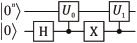
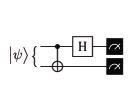
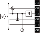
Concrete circuit representations of these measurement operators are given in Table 1. A nice property of these measurement operators is that each of them contains at most n1n-1 CNOT gates, which is suitable for the NISQ devices. We refer to the present method as the extended Bell measurements (XBMs) because the measurement operators MRe(b,c)M^{(b,c)}_{\rm Re} and MIm(b,c)M^{(b,c)}_{\rm Im} are similar to those for the Bell measurements except for the number of CNOT gates.
(a)
(b)

Figure 1: Typical circuits for (a) standard Bell measurements, and (b) extended Bell measurements.

In Fig.1, typical circuits for a standard Bell measurements and the extended Bell measurements are shown.

Simultaneous Measurements (Lines 3–4 of Eq. (2.2))

We proved the following theorem.

Theorem 1

If bc=bcb\oplus c=b^{\prime}\oplus c^{\prime} and bcb^{\prime}\neq c^{\prime}, then MRe(b,c)=MRe(b,c)M^{(b,c)}_{\rm Re}=M^{(b^{\prime},c^{\prime})}_{\rm Re} and MIm(b,c)=MIm(b,c)M^{(b,c)}_{\rm Im}=M^{(b^{\prime},c^{\prime})}_{\rm Im}.

The proof is given in Appendix A.2. The above theorem states that the number of distinct measurement operators can be drastically reduced. In addition, the superscript ()(b,c)(\bullet)^{(b,c)} can be replaced with ()(bc)(\bullet)^{(b\oplus c)} because each distinct measurement operator is identified by bcb\oplus c. Reformulation leads to the fourth line of Eq. (2.2).

Operator Selecting Model (Lines 4–5 of Eq. (2.2))

The fourth line of Eq. (2.2) does not seem to express an expectation value because it does not take the form iaiP(a^=ai)\sum_{i}a_{i}P(\hat{a}=a_{i}). Here, we introduce an operator selecting model p(l,s)p(l,s) that represents the probability of selecting the measurement operator Ms(l)M^{(l)}_{s}, where l𝒮(A)l\in\mathcal{S}(A) and s{Re,Im}s\in\{{\rm Re},{\rm Im}\}. Here, 𝒮(A)\mathcal{S}(A) is a set of bcb\oplus c where AbcA_{bc} has non-zero components, as defined in Table 1. Introducing p(l,s)p(l,s), φ|A|φ\langle\varphi|A|\varphi\rangle is eventually represented as on the rightmost side of Eq. (2.2) and takes the form iaiP(a^=ai)\sum_{i}a_{i}P(\hat{a}=a_{i}). Although the concrete description of p(l,s)p(l,s) is arbitrary the appropriate definition of p(l,s)p(l,s) reduces the variance of the expectation estimation.

When we regard Eq. (2.2) as expressing the expectation value in a stochastic process, an event is selecting a measurement operator Ms(l)M^{(l)}_{s} with probability p(l,s)p(l,s) followed by measuring a bit-string bb of a state Ms(l)|φM^{(l)}_{s}|\varphi\rangle in the computational basis, and then obtaining a corresponding outcome. Denoting a complex random variable corresponding to such an event as a^\hat{a}, we have

𝔼l,s,bp(l,s,b)[a^]=φ|A|φ.\displaystyle{\mathbb{E}}_{l,s,b\sim p(l,s,b)}[\hat{a}]=\langle\varphi|A|\varphi\rangle. (9)

In the following, we simply express 𝔼l,s,bp(l,s,b)[a^]{\mathbb{E}}_{l,s,b\sim p(l,s,b)}[\hat{a}] as 𝔼p[a^]{\mathbb{E}}_{p}[\hat{a}].

Significance of Eq. (2.2)

There are three important aspects to the expression in Eq. (2.2).

  1. 1.

    There are fewer distinct measurement operators.

  2. 2.

    Each measurement operator has a simple explicit expression.

  3. 3.

    There are fewer CNOT gates in each measurement operator.

Equation (2.2) contains only |𝒮(A)×{Re,Im}||\mathcal{S}(A)\times\{{\rm Re},{\rm Im}\}| measurement operators, II, {MRe(l)}l𝒮(A){0n}\{M^{(l)}_{\rm Re}\}_{l\in\mathcal{S}(A){\color[rgb]{0,0,0}\setminus\{0^{n}\}}}, and {MIm(l)}l𝒮(A){0n}\{M^{(l)}_{\rm Im}\}_{l\in\mathcal{S}(A){\color[rgb]{0,0,0}\setminus\{0^{n}\}}}. The number of distinct measurement operators depends on the structure of AA, which is discussed further in Sec. 3. A simple explicit expression of each measurement operator is beneficial from the viewpoint of time complexity for circuit construction. The number of CNOT gates included in each measurement operator is at most n1n-1, which is suitable for the NISQ device because most of the real-device error comes from two-qubit entangling gates. In summary, qualitatively speaking, the construction of measurement operators is fast and the evaluation error on a real quantum computer using these operators is expected to be small. Further details of the complexity analyses are given in Sec. 3.

2.3 Upper Bound of Variance

An upper bound of the variance of a^\hat{a} associated with the XBM can be easily calculated as

Varp[a^]\displaystyle{\rm Var}_{p}[\hat{a}] =𝔼p[|a^|2]|𝔼p[a^]|2\displaystyle={\mathbb{E}}_{p}[|\hat{a}|^{2}]-|{\mathbb{E}}_{p}[\hat{a}]|^{2}
𝔼p[|a^|2]\displaystyle\leq{\mathbb{E}}_{p}[|\hat{a}|^{2}]
=l,s,b|a(l,s,b)|2p(l,s,b),\displaystyle=\sum_{l,s,b}|a(l,s,b)|^{2}p(l,s,b), (10)

which depends on the operator selecting model p(l,s)p(l,s). A simple choice of p(l,s)p(l,s) is a uniform distribution over ll and ss whereas a more sophisticated choice can reduce the variance of a^\hat{a} (see Appendix B for details).

Here, we assume that |A|max2=O(tr(A2)/q)|A|^{2}_{\max}=O({\rm tr}(A^{2})/q) where |A|max:=maxb,c{|Abc|}|A|_{\max}:=\max_{b,c}\{|A_{bc}|\} is the maximum norm of AA and qq the number of non-zero components of AA, respectively. Under this assumption, no matter which operator selecting model is used, the upper bound of the variance of a^\hat{a} can be roughly estimated as

Varp[a^]m2|A|max2=O(m2qtr(A2))\displaystyle{\color[rgb]{0,0,0}{\rm Var}_{p}[\hat{a}]\leq m^{2}|A|^{2}_{\max}=O\Bigg(\frac{m^{2}}{q}{\rm tr}(A^{2})\Bigg)} (11)

where

m:=|𝒮(A)×{Re,Im}|\displaystyle{\color[rgb]{0,0,0}m:=|\mathcal{S}(A)\times\{{\rm Re},{\rm Im}\}|} (12)

is the number of distinct measurement operators (see Appendix C.2 for details).

2.4 Relationship with the Classical Shadow

Our method is closely related to the classical shadow with random Clifford measurements [31]. The main differences are the unitary ensemble and the operator selecting model. The random Clifford circuits are used in the classical shadow whereas mm distinct measurement operators are used in the XBM. In addition, only the uniform operator selecting model is considered in the original classical shadow whereas an arbitrary operator selecting model is considered in the XBM.

Additionally, the number of two-qubit entangling gates in each measurement operator is different. The classical shadow with random Clifford measurements requires O(n2/log(n))O(n^{2}/\log(n)) two-qubit entangling gates for each measurement operator whereas the XBM requires at most n1n-1 CNOT gates for each.

The upper bound of the variance associated with the classical shadow with the random Clifford measurements is O(tr(A2))O({\rm tr}(A^{2})) [31]. Hence, when m2qm^{2}\ll q, our method has an upper bound tighter than that of the classical shadow. An example of this case is that non-zero components of AA are densely filled in the tight bandwidth. When the bandwidth of AA is k=O(nc)k=O(n^{c}), and the non-zero components are densely filled in the band,

Varp[a^]=O(nc+12ntr(A2))\displaystyle{\rm Var}_{p}\big[\hat{a}\big]=O\Bigg(\frac{n^{c+1}}{2^{n}}{\rm tr}(A^{2})\Bigg) (13)

(see Appendix C.2 for other cases). Such a matrix frequently appear in the case of the FEM as mentioned in the introduction. In this case, the adoption of our method exponentially improves the variance relative to the classical shadow.

The relationship between the XBM and classical shadow is further discussed in Appendix D, which gives the explicit form of the classical shadow associated with the XBM method.

3 Algorithm and Complexity

input : Non-zero matrix elements and corresponding indices, {b,c,Abc|Abc0}\{b,c,A_{bc}|A_{bc}\neq 0\}
output : Measurement operators Ms(l)M^{(l)}_{s} and outcomes α(l,s,b)\alpha(l,s,b)
initialize : Ms(l)NoneM^{(l)}_{s}\leftarrow\texttt{None} and α(l,s,b)0\alpha(l,s,b)\leftarrow 0 for all l,s,bl,s,b
for (b,c){(b,c)|Abc0}(b,c)\in\{(b,c)|A_{bc}\neq 0\} do
lbcl\leftarrow b\oplus c
if l0nl\neq 0^{n} then
 j0(l)max{j|lj=1}j^{(l)}_{0}\leftarrow\max\{j|l_{j}=1\}
end if
 /* Compute and store measurement operators */
 if Measurement operators MRe(l)M^{(l)}_{\rm Re} and MIm(l)M^{(l)}_{\rm Im} have not yet been computed then
 if l=0nl=0^{n} then
    MRe(l)IM^{(l)}_{\rm Re}\leftarrow I else
    MRe(l),MIm(l)M^{(l)}_{\rm Re},\,M^{(l)}_{\rm Im}\leftarrow (see Table 1)
end if
      end if
 /* Compute and store outcomes */
 if b=cb=c then
 α(l,Re,b)α(l,Re,b)+Abc\alpha(l,{\rm Re},b)\leftarrow\alpha(l,{\rm Re},b)+A_{bc}
else if b<cb<c then
 b¯b2j0(l)\bar{b}\leftarrow b\oplus 2^{j^{(l)}_{0}}
α(l,Re,b)α(l,Re,b)+Abc/2\alpha(l,{\rm Re},b)\leftarrow\alpha(l,{\rm Re},b)+A_{bc}/2
α(l,Re,b¯)α(l,Re,b¯)Abc/2\alpha(l,{\rm Re},\bar{b})\leftarrow\alpha(l,{\rm Re},\bar{b})-A_{bc}/2
α(l,Im,b)α(l,Im,b)+iAbc/2\alpha(l,{\rm Im},b)\leftarrow\alpha(l,{\rm Im},b)+{\rm i}A_{bc}/2
α(l,Im,b¯)α(l,Im,b¯)iAbc/2\alpha(l,{\rm Im},\bar{b})\leftarrow\alpha(l,{\rm Im},\bar{b})-{\rm i}A_{bc}/2
else if b>cb>c then
 c¯c2j0(l)\bar{c}\leftarrow c\oplus 2^{j^{(l)}_{0}}
α(l,Re,c)α(l,Re,c)+Abc/2\alpha(l,{\rm Re},c)\leftarrow\alpha(l,{\rm Re},c)+A_{bc}/2
α(l,Re,c¯)α(l,Re,c¯)Abc/2\alpha(l,{\rm Re},\bar{c})\leftarrow\alpha(l,{\rm Re},\bar{c})-A_{bc}/2
α(l,Im,c)α(l,Im,c)iAbc/2\alpha(l,{\rm Im},c)\leftarrow\alpha(l,{\rm Im},c)-{\rm i}A_{bc}/2
α(l,Im,c¯)α(l,Im,c¯)+iAbc/2\alpha(l,{\rm Im},\bar{c})\leftarrow\alpha(l,{\rm Im},\bar{c})+{\rm i}A_{bc}/2
end if
   end for
Algorithm 1 Algorithm for term grouping in the XBM method
input : Number of shots NN, operator selecting model p(l,s)p(l,s), measurement operators {Ms(l)}\{M^{(l)}_{s}\}, quantum state |φ|\varphi\big>, outcomes {α(l,s,b)}\{\alpha(l,s,b)\}
output : Expectation value xx
for i=1i=1 to NN do
/* Pick a measurement operator */
 l,sp(l,s)l,s\sim p(l,s) ;
 // Classical computing
 MMs(l)M\leftarrow M^{(l)}_{s} ;
 // Access to the classical memory
 /* Measure a bit string and update xx */
 b|b|M|φ|2b\sim|\langle b|M|\varphi\rangle|^{2} ;
 // Quantum computing
 xiα(l,s,b)x_{i}\leftarrow\alpha(l,s,b) ;
 // Access to the classical memory and classical computing
   end for
xixi/Nx\leftarrow\sum_{i}x_{i}/N ;
// Take arithmetic mean
Algorithm 2 Algorithm for calculating an expectation value in the XBM method. Note that median-of-means or others can be used instead of the arithmetic mean in the last line.

The algorithms for term grouping and calculating an expectation value using the XBM method are presented as Algorithms 1 and 2, respectively. These algorithms follow the equations described in Eq. (2.2) (see Appendix A for details). The greatest advantage of the proposed method, the XBM method, is that the number of unique circuits required to estimate ψ0|A|ψ1\big<\psi_{0}\big|A\big|\psi_{1}\big> can be rapidly reduced. In this section, the reduction ratio of the number of unique circuits and the computational cost of the XBM method are discussed.

3.1 Number of Distinct Operators

In this paper, an ss-sparse matrix and band matrix with bandwidth kk are defined as follows.

Definition 1 (ss-sparse matrix AA [35])

A2n×2nA\in{\mathbb{C}}^{2^{n}\times 2^{n}} is ss-sparse if each column has at most ss nonzero entries.

Definition 2 (band matrix AA)

A2n×2nA\in{\mathbb{C}}^{2^{n}\times 2^{n}} is a band matrix with bandwidth kk if Aij=0A_{ij}=0 for all i,ji,j such that |ij|>k|i-j|>k.

According to these definitions, the following theorems hold.

Theorem 2 (ss-sparse matrix AA)

Let A2n×2nA\in{\mathbb{C}}^{2^{n}\times 2^{n}} and |ψ0,|ψ12n\big|\psi_{0}\big>,\big|\psi_{1}\big>\in{\mathbb{C}}^{2^{n}}. When AA is an ss-sparse matrix, there exists an algorithm such that the number of quantum circuits required to evaluate ψ0|A|ψ1\big<\psi_{0}\big|A\big|\psi_{1}\big> is 2n+12^{n+1} in the worst case.

Theorem 3 (band matrix AA)

Let A2n×2nA\in{\mathbb{C}}^{2^{n}\times 2^{n}} and |ψ0,|ψ12n\big|\psi_{0}\big>,\big|\psi_{1}\big>\in{\mathbb{C}}^{2^{n}}. When the bandwidth of AA is k>0k>0, there exists an algorithm such that the number of quantum circuits required to evaluate ψ0|A|ψ1\big<\psi_{0}\big|A\big|\psi_{1}\big> is 2((nr)k+2r)2((n-r)k+2^{r}) in the worst case where r=log2kr=\lceil\log_{2}k\rceil.

Here, we define the upper bound of the number of the unique circuits for an nn-qubit system with bandwidth kk as

m¯(n,k)\displaystyle\overline{m}(n,k) :={2((nr)k+2r)k>01k=0\displaystyle:=\left\{\begin{array}[]{ll}2((n-r)k+2^{r})&k>0\\[14.22636pt] 1&k=0\end{array}\right.

where r:=log2kr:=\lceil\log_{2}k\rceil. Note that when evaluating φ|A|φ\langle\varphi|A|\varphi\rangle whose AA has non-zero diagonal components, the upper bound can be reduced to 2((nr)k+2r)12((n-r)k+2^{r})-1 for k>1k>1 (see Appendix E.2).

The proofs are given in Appendix E. Note that a fully dense matrix can be viewed as a 2n2^{n}-sparse matrix or a band matrix with bandwidth k=2n1k=2^{n}-1.

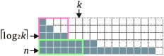
Unfortunately, we find that the evaluation of the number of circuits in Algorithm 1 is tight; i.e., there exists an ss-sparse matrix that requires 2n+12^{n+1} unique circuits, which is the same as the case for the fully dense matrix. However, if AA is a band matrix, then at least the number of unique circuits required to estimate ψ0|A|ψ1\big<\psi_{0}\big|A\big|\psi_{1}\big> can be reduced to 2((nr)k+2r)2((n-r)k+2^{r}), where kk is the bandwidth and r=log2kr=\lceil\log_{2}k\rceil. When AA is sufficiently tight (i.e., bandwidth k=O(nc)k=O(n^{c})), 2((nr)k+2r)=O(nc+1)2((n-r)k+2^{r})=O(n^{c+1}). Note that the number of unique Pauli strings required to evaluate ψ0|A|ψ1\big<\psi_{0}\big|A\big|\psi_{1}\big> using naïve Pauli measurements is 2n+1((nr)k+2r)2^{n+1}((n-r)k+2^{r}) (see Sec. E.4). The XBM thus outperforms the naïve Pauli measurements in terms of the number of unique circuits required to evaluate ψ0|A|ψ1\big<\psi_{0}\big|A\big|\psi_{1}\big>. This exponential improvement is due to the difference in the basis of AA, but the number of unique circuits when using the XBM method does not appreciably increase even if AA is represented in the Pauli basis (see Sec. E.5).

As mentioned before, our method is the generalization of [7]. In their formulation, both φ|A2|φ=φ|(B+C(0)+C(1))|φ\langle\varphi|A^{2}|\varphi\rangle=\langle\varphi|(B+C^{(0)}+C^{(1)})|\varphi\rangle and b|A|φ\langle b|A|\varphi\rangle are calculated to solve the one-dimensional Poisson equation, and the numbers of unique circuits required to evaluate φ|A2|φ=φ|(B+C(0)+C(1))|φ\langle\varphi|A^{2}|\varphi\rangle=\langle\varphi|(B+C^{(0)}+C^{(1)})|\varphi\rangle and b|A|φ\langle b|A|\varphi\rangle are 4n+14n+1 and 2n+12n+1, respectively, where the bandwidth of BB, C(0)C^{(0)}, C(1)C^{(1)} and AA are 22, 00, 00 and 11, respectively. This is consistent with m¯(n,k=2)+m¯(n,k=0)+m¯(n,k=0)=4n+1+1=4n+2\overline{m}(n,k=2)+\overline{m}(n,k=0)+\overline{m}(n,k=0)=4n+1+1=4n+2 and m¯(n,k=1)=2n+2\overline{m}(n,k=1)=2n+2 (see Eq. (3.1)), where the +1+1 difference comes from the counting of an unnecessary term, Im(φ|bb|φ)=0{\rm Im}\big(\langle\varphi|b\rangle\langle b|\varphi\rangle\big)=0.

3.2 Time Complexity for Term Grouping

We assume that data {(b,c,Abc)|Abc0}\{(b,c,A_{bc})|A_{bc}\neq 0\} are stored in the memory of the classical computer, where AbcA_{bc} is the (b,c)(b,c) component of the matrix AA. For each (b,c){(b,c)|Abc0}:=(b,c)\in\{(b,c)|A_{bc}\neq 0\}:=\mathcal{B}, bit strings to be measured are calculated from bb and j0(bc)=max{j|(bc)j=1}j^{(b\oplus c)}_{0}=\max\{j|(b\oplus c)_{j}=1\} for bcb\neq c. The computational cost of calculating j0(bc)j^{(b\oplus c)}_{0} with classical computers is O(n)O(n), and the total time complexity for term grouping is thus O(nd)O(nd), where dd is the size of \mathcal{B}, which is the number of non-zero elements of AA.

Note that in Algorithm 1, measurement operators Ms(l)M^{(l)}_{s} are simultaneously calculated with term grouping. Each measurement circuit can be built in O(n)O(n) time (see definition of Ms(l)M^{(l)}_{s} in Table 1), and its calculation is only carried out when Ms(l)M^{(l)}_{s} is not yet calculated. Therefore, the total time complexity of building measurement circuits is O(nm)O(nm) where mdm\leq d is the number of distinct bcb\oplus c values among (b,c)(b,c) pairs with non-zero AbcA_{bc} values, which does not affect the total time complexity of term grouping.

3.3 Gate Counts for Measurement Circuits

As described in Table 1, the maximum number of gate counts is n+1n+1 for each unique circuit; i.e., there are n1n-1 CNOT gates, one Hadamard gate and one phase gate. Hence, the gate count for each measurement circuit is O(n)O(n).

4 Experiments

We implement our model with Qiskit version 0.25.0 [34]. All experiments are carried out on a single Intel(R) Core(TM) i9-9900X CPU @ 3.50GHz and ibm_kawasaki of an IBM-Q system. To compare with the existing methods, QWC (qubit–wise commuting) [27, 28, 21] and GC (general commuting) [24] are conducted with the same machine. The Python function, group_into_tensor_product_basis_sets, implemented in OpenFermion [36], is used for QWC whereas Python code provided by one of the authors of [24] is used for GC. In GC, the Bron-Kerbosch algorithm [37] is used to solve the minimum clique covering problem.

In our method, the XBM method, Re(φ|bc|φ){\rm Re}(\big<\varphi\big|b\big>\big<c\big|\varphi\big>) and Im(φ|bc|φ){\rm Im}(\big<\varphi\big|b\big>\big<c\big|\varphi\big>) can be separately evaluated. To take this advantage, we consider the two following cases in which Im(φ|bc|φ){\rm Im}(\big<\varphi\big|b\big>\big<c\big|\varphi\big>) does not need to be estimated.

  1. 1.

    A2n×2nA\in{\mathbb{R}}^{2^{n}\times 2^{n}} and only Re(ψ0|A|ψ1){\rm Re}(\big<\psi_{0}\big|A\big|\psi_{1}\big>) is required. For example, AA is real symmetric matrix and |ψ0=|ψ1\big|\psi_{0}\big>=\big|\psi_{1}\big>.

  2. 2.

    ϕ0,ϕ1\exists\phi_{0},\phi_{1} s.t. eiϕ0|ψ0,eiϕ1|ψ12ne^{{\rm i}\phi_{0}}\big|\psi_{0}\big>,e^{{\rm i}\phi_{1}}\big|\psi_{1}\big>\in{\mathbb{R}}^{2^{n}}

In these cases, only Re(φ|bc|φ){\rm Re}(\big<\varphi\big|b\big>\big<c\big|\varphi\big>) needs to be estimated because

Re(φ|A|φ)=b,cRe(Abc)Re(φ|bc|φ)\displaystyle{\rm Re}\Big(\big<\varphi\big|A\big|\varphi\big>\Big)=\sum_{b,c}{\rm Re}\Big(A_{bc}\Big){\rm Re}\Big(\big<\varphi\big|b\big>\big<c\big|\varphi\big>\Big)
b,cIm(Abc)Im(φ|bc|φ)\displaystyle\hskip 36.98857pt-\sum_{b,c}{\rm Im}\Big(A_{bc}\Big){\rm Im}\Big(\big<\varphi\big|b\big>\big<c\big|\varphi\big>\Big)

and

Im(φ|A|φ)=b,cIm(Abc)Re(φ|bc|φ)\displaystyle{\rm Im}\Big(\big<\varphi\big|A\big|\varphi\big>\Big)=\sum_{b,c}{\rm Im}\Big(A_{bc}\Big){\rm Re}\Big(\big<\varphi\big|b\big>\big<c\big|\varphi\big>\Big)
+b,cRe(Abc)Im(φ|bc|φ).\displaystyle\hskip 36.98857pt+\sum_{b,c}{\rm Re}\Big(A_{bc}\Big){\rm Im}\Big(\big<\varphi\big|b\big>\big<c\big|\varphi\big>\Big).

The computational cost is reduced by half in these cases and we thus refer these to these cases by “XBM (half)” in the following. Note that in the case that A2n×2nA\in{\mathbb{C}}^{2^{n}\times 2^{n}} and |ψ0,|ψ12n\big|\psi_{0}\big>,\big|\psi_{1}\big>\in{\mathbb{C}}^{2^{n}}, even if |ψ0=|ψ1\big|\psi_{0}\big>=\big|\psi_{1}\big> and AA is an Hermitian matrix, which is the case that ψ0|A|ψ1\big<\psi_{0}\big|A\big|\psi_{1}\big>\in{\mathbb{R}}, both Re(φ|bc|φ){\rm Re}(\big<\varphi\big|b\big>\big<c\big|\varphi\big>) and Im(φ|bc|φ){\rm Im}(\big<\varphi\big|b\big>\big<c\big|\varphi\big>) have to be evaluated.

2|01|A2\big|0\big>\big<1\big|\otimes A (Eq. (A.1)) is used instead of AA when evaluating the case that |ψ0|ψ1\big|\psi_{0}\big>\neq\big|\psi_{1}\big>. In QWC and GC, the matrix AA is converted to the sum of the Pauli bases before adopting the term grouping algorithms.

4.1 Term Grouping

4.1.1 Setups

We first show that the present method is more efficient in terms of both the number of unique circuits and the computational cost for term grouping than existing methods. We conduct the following three experiments:

  1. 1.

    We compare the number of unique circuits and time required for term grouping between different methods when |ψ0=|ψ1\big|\psi_{0}\big>=\big|\psi_{1}\big>.

  2. 2.

    We repeat the first experiment but for |ψ0|ψ1\big|\psi_{0}\big>\neq\big|\psi_{1}\big>.

  3. 3.

    We estimate the number of unique circuits for the XBM method when the non-zero elements of AA are randomly placed.

In the first and second experiments, all components of A2n×2nA\in{\mathbb{C}}^{2^{n}\times 2^{n}} are randomly set to non-zero values. AA is then restricted to be a band matrix by setting Abc=0A_{bc}=0 for |bc|>k|b-c|>k, where k=0,1,,2n1k=0,1,\cdots,2^{n-1}. In the third experiment, we observe the term groupings while changing the number of non-zero elements, dd, that are randomly placed in AA. The number of unique circuits is obtained 10 times for each value of dd. The mean and standard deviation are then calculated.

4.1.2 Results
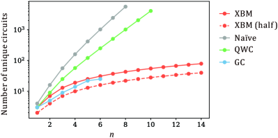
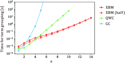
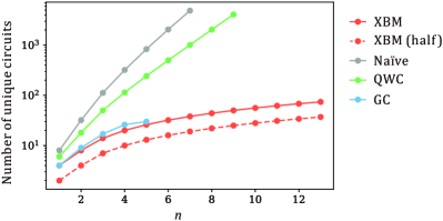
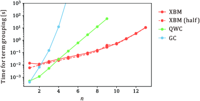
Figure 2: Number of unique circuits in estimating ψ0|A|ψ1\big<\psi_{0}\big|A\big|\psi_{1}\big> and the time required for term grouping when the bandwidth of AA is k=3k=3: (a)(b) |ψ0=|ψ1\big|\psi_{0}\big>=\big|\psi_{1}\big>; (c)(d) |ψ0|ψ1\big|\psi_{0}\big>\neq\big|\psi_{1}\big>. XBM: present method, XBM (half): present method but only evaluating the real part of φ|bc|φ\langle\varphi|b\rangle\langle c|\varphi\rangle, Naïve: Pauli measurements without term grouping, QWC: Pauli measurements with grouping associated with the qubit-wise commutativity [27, 28, 21], GC: Pauli measurements with grouping associated with the general commutativity [24].
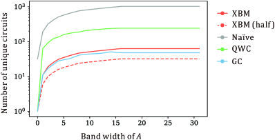
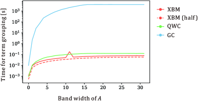
Figure 3: Number of unique circuits in estimating ψ0|A|ψ0\big<\psi_{0}\big|A\big|\psi_{0}\big> and the time required for term grouping with respect to the bandwidth of AA, for a five-qubit system. XBM: present method, XBM (half): present method but only evaluating the real part of φ|bc|φ\langle\varphi|b\rangle\langle c|\varphi\rangle, Naïve: Pauli measurements without term grouping, QWC: Pauli measurements with grouping associated with the qubit-wise commutativity [27, 28, 21], GC: Pauli measurements with grouping associated with the general commutativity [24].
Experiment 1

Figure 2 shows the dependency of the number of unique circuits on nn, in the case that |ψ0=|ψ1\big|\psi_{0}\big>=\big|\psi_{1}\big> and the bandwidth k=3k=3. The XBM and GC results have similar tendencies that are much better than the tendencies of Naïve and QWC in terms of the reduction ratio of the unique circuits. When the imaginary part of φ|bc|φ\big<\varphi|b\big>\big<c\big|\varphi\big> is not required, as in the case of XBM (half), the number of unique circuits is lower for the XBM method than for the GC method.

Figure 2 shows the dependency of the computational time for term grouping on nn when the bandwidth k=3k=3. Obviously, the XBM method is much faster than all other methods for large nn. This is because GC and QWC methods heuristically solve a minimum clique cover problem that is NP-hard, whereas the XBM method analytically groups the terms as shown in Sec. 2. Note that this qualitative tendency of the comparison results does not change for any bandwidth as shown in Fig. 3 and Fig. 3.

Experiment 2

Figures 2 and 2 show the results for the case that |ψ0|ψ1\big|\psi_{0}\big>\neq\big|\psi_{1}\big>. In this case, regardless of whether the imaginary part of φ|bc|φ\big<\varphi\big|b\big>\big<c\big|\varphi\big> is required, the number of unique circuits is lower for the XBM method than for all other methods. This is because the number of unique circuits for |01|2A\big|0\big>\big<1\big|\otimes 2A is the same as that for AA for the XBM method, but not for the other methods. The tendency of the time required for term grouping against nn in the case that |ψ0|ψ1\big|\psi_{0}\big>\neq\big|\psi_{1}\big> is the same as that in the case that |ψ0=|ψ1\big|\psi_{0}\big>=\big|\psi_{1}\big>.


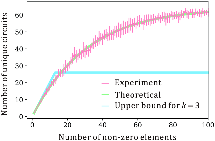
Figure 4: Results when the non-zero elements of AA are randomly placed for the five-qubit system. Red and green lines are the experimental and analytic results of the XBM, respectively. The blue line is the upper bound when all non-zero elements are placed in a k=3k=3 band, min(d,m¯(5,3))=min(d,2((5log23)3+2log23))\min(d,\overline{m}(5,3))=\min(d,2((5-\lceil\log_{2}3\rceil)\cdot 3+2^{\lceil\log_{2}3\rceil}))
Experiment 3

The third experiment is carried out to show that the XBM method is more efficient in terms of the number of unique circuits when AA is a band-matrix. Figure 4 shows the results of the number of unique circuits for the XBM method when the non-zero elements of AA are randomly placed; this case is referred to as random-A. The upper bound of the number of unique circuits when AA is a band-matrix with a bandwidth k=3k=3 is also shown in the figure (blue line); this case is referred to as band-A.

The number of unique circuits required to evaluate random-A is analytically derived as follows. Let AA have dd non-zero elements at random. Here, we consider a box that contains a total of N2N^{2} balls of NN types, where N=2nN=2^{n}. In fact, the number of unique circuits is twice the expectation number of ball types when one samples dd balls from the box. The probability that the balls are of type kk when dd balls are sampled from a box containing a total of N2N^{2} balls of NN types, P(k,d,N)P(k;d,N), is

P(k,d,N)=𝔑(k,d,N)CdN2\displaystyle{P(k;d,N)=\frac{\mathfrak{N}(k,d,N)}{{}_{N^{2}}{\rm C}_{d}}}

where

𝔑(k,d,N)=CkNCdkN\displaystyle{\mathfrak{N}(k,d,N)={}_{N}{\rm C}_{k}\ {}_{kN}{\rm C}_{d}\hskip 56.9055pt}
i=1k1CkNCikCiN𝔑(i,d,N).\displaystyle{\hskip 56.9055pt-\sum^{k-1}_{i=1}\frac{{}_{N}{\rm C}_{k}\ {}_{k}{\rm C}_{i}}{{}_{N}{\rm C}_{i}}\mathfrak{N}(i,d,N).}

The expectation value is then given as

E(d,N)=k=1dkP(k,d,N).\displaystyle{E(d,N)=\sum^{d}_{k=1}kP(k;d,N).}

The green line in Fig. 4 denotes the expectation value E(d,N=25)E(d,N=2^{5}) and is consistent with the red line, which is the mean of the experimental results. The figure shows that the number of unique circuits for random-A is much larger than that for band-A when the number of nonzero elements of AA is sufficiently large. For example, when d=50d=50, the expectation number of unique circuits for random-A is approximately 52. Meanwhile, the number of unique circuits is at most 2626 when all 50 non-zero elements are put into a bandwidth k=3k=3. This indicates that adoption of the XBM method can reduce the number of unique circuits more efficiently when the bandwidth of AA is narrower.

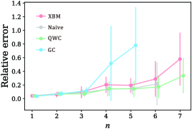
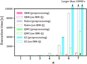
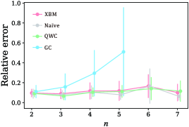
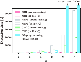
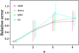
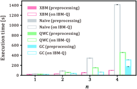
Figure 5: Results of the real device evaluation of ψ0|A|ψ1\big<\psi_{0}\big|A\big|\psi_{1}\big>. (a)(b) |ψ0=|ψ1\big|\psi_{0}\big>=\big|\psi_{1}\big>; (c)(d) |ψ0=|ψ1\big|\psi_{0}\big>=\big|\psi_{1}\big> and k=3k=3; (e)(f) |ψ0|ψ1\big|\psi_{0}\big>\neq\big|\psi_{1}\big>. XBM: present method, Naïve: Pauli measurements without term grouping, QWC: Pauli measurements with grouping associated with the qubit-wise commutativity [27, 28, 21], GC: Pauli measurements with grouping associated with the general commutativity [24]. method (preprocessing) and method (on IBM-Q) denote the execution time of classical preprocessing required before quantum processing and of quantum processing on the IBM-Q system, respectively.

4.2 Real-device Experiments

4.2.1 Setups

In real-device experiments, we use the uniform operator selecting model p(l,s)=1/mp(l,s)=1/m. For simplicity, all measurement operators are used at once instead of sampling ll and ss. We set the number of shots for each measurement operator at 8192, which is the maximum number for the IBM-Q system. We use the ibm_kawasaki backend for all real-device experiments because its CNOT error and readout error are smaller than those of other backends. Both the elapsed wall time for preprocessing and execution time on the IBM-Q system are recorded. Here, preprocessing includes term grouping, calculating the coefficients of Pauli bases, building measurement circuits, and all other calculations conducted on a classical computer before carrying out quantum computing.

We conduct four real device experiments.

  1. 1.

    We compare the relative errors of ψ0|A|ψ1\big<\psi_{0}\big|A\big|\psi_{1}\big> and execution time for each method when |ψ0=|ψ1\big|\psi_{0}\big>=\big|\psi_{1}\big>.

  2. 2.

    We evaluate the relative errors of φ|Abc|φ\big<\varphi\big|A_{bc}\big|\varphi\big> where AbcA_{bc} has only one non-zero element in the bbth row and ccth column.

  3. 3.

    We compare the relative errors of ψ0|A|ψ1\big<\psi_{0}\big|A\big|\psi_{1}\big> and execution time for each method when AA is a band matrix and |ψ0=|ψ1\big|\psi_{0}\big>=\big|\psi_{1}\big>.

  4. 4.

    We repeat the first experiment, but |ψ0|ψ1\big|\psi_{0}\big>\neq\big|\psi_{1}\big>.

Here, we define the relative errors as

|ψ0|A|ψ1realdeviceψ0|A|ψ1GT||ψ0|A|ψ1GT|\displaystyle{\frac{\Big|\big<\psi_{0}\big|A\big|\psi_{1}\big>_{\rm real\ device}-\big<\psi_{0}\big|A\big|\psi_{1}\big>_{\rm GT}\Big|}{\Big|\big<\psi_{0}\big|A\big|\psi_{1}\big>_{\rm GT}\Big|}}

where ()realdevice(\bullet)_{\rm real\ device} and ()GT(\bullet)_{\rm GT} are the evaluation value of ()(\bullet) on the real device and the ground truth of ()(\bullet), respectively.

In the first, third and fourth experiments, all the components of AA are randomly set as Re(Abc),Im(Abc)[100,100]{\rm Re}(A_{bc}),{\rm Im}(A_{bc})\in[-100,100]. In preparing |ψ0\big|\psi_{0}\big> and |ψ1\big|\psi_{1}\big>, RxR_{x}, RyR_{y} and RzR_{z} gates are randomly set for each qubit. The experiments are carried out 10 times for each condition, and the mean and standard deviation of the results are calculated.

In the second experiment, only one component, AbcA_{bc}, is set to be non-zero (i.e., Re(Abc),Im(Abc)[100,100]{\rm Re}(A_{bc}),{\rm Im}(A_{bc})\in[-100,100]), whereas all other components are set to zero. Unlike the case in the other experiments, |φ\big|\varphi\big> is prepared by acting on all qubits with Hadamard gates to mitigate the effect of the randomness of the |φ\big|\varphi\big> preparation. This experiment is repeated for b=0,1,,2n1b=0,1,\cdots,2^{n}-1 and c=0,1,,2n1c=0,1,\cdots,2^{n}-1. As a result, the relative errors for all components of AA are obtained. Only XBM and Naïve experiments are carried out here. The experiments are carried out 10 times for each (b,c)(b,c), and the mean results are calculated.

4.2.2 Results

Experiment 1

As shown in Fig. 5, the relative errors of the XBM method are much better than those of the GC method but worse than those of the Naïve and QWC methods for n4n\geq 4 when |ψ0=|ψ1\big|\psi_{0}\big>=\big|\psi_{1}\big>. This trend can be explained by the circuit complexity. The XBM method uses multiple CNOT gates whereas the Naïve and QWC methods do not, and the circuit for the GC method is much more complex than the circuits of the other methods. Although the XBM method is slightly inferior in terms of the relative error compared with the Naïve and QWC methods, the total execution time for the XBM method is much shorter than the times for the other methods (Fig. 5). The execution time on a real device for the XBM method is slightly longer than that for the GC method, which depends on the number of unique circuits. However, the total execution time for the XBM method is much shorter than that for the GC method because the XBM method performs term grouping much more rapidly than the GC method. In the case of the XBM method, the execution time for term grouping is negligible compared with the execution time on the IBM-Q system. In summary, the proposed method, namely the XBM method, can evaluate ψ0|A|ψ0\big<\psi_{0}\big|A\big|\psi_{0}\big> with slightly worse accuracy than the Naïve and QWC methods but in much less time.
Refer to caption
Refer to caption
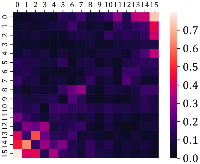
Figure 6: Element-wise relative errors of φ|Arc|φ\big<\varphi\big|A_{rc}\big|\varphi\big> for a four-qubit system evaluated on a real device: (a) XBM method; (b) Naïve method.
Experiment 2

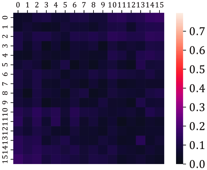
Figure 6 compares the elementwise relative error between the XBM and Naïve methods. In the case of the XBM method, the relative errors are larger for the anti-diagonal components than for the other components, whereas all components have similar relative errors in the case of the Naïve method. This result is consistent with that of the XBM method using the most CNOT gates in the evaluation of anti-diagonal components. Note that the number of CNOT gates required for the XBM method to evaluate the (b,c)(b,c) component of AA is

max(0,i=02n1bici1).\max\Bigg(0,\sum^{2^{n}-1}_{i=0}b_{i}\oplus c_{i}-1\Bigg).

This indicates that the XBM method can evaluate ψ0|A|ψ0\big<\psi_{0}\big|A\big|\psi_{0}\big> with much smaller error when AA is a band matrix.

Experiment 3

Figure 5 shows that the relative errors of the XBM, Naïve and QWC methods are small in the case that AA is a band matrix; the errors approximately range 0.10.150.1-0.15 and they are all comparable for at least n7n\leq 7. Meanwhile, the XBM method can evaluate ψ0|A|ψ0\big<\psi_{0}\big|A\big|\psi_{0}\big> much more rapidly than the Naïve and QWC methods (Fig. 5). It is thus concluded that the XBM method can evaluate ψ0|A|ψ0\big<\psi_{0}\big|A\big|\psi_{0}\big> with the same accuracy as the Naïve and QWC methods and in a much shorter time when AA is a band matrix.

Experiment 4

Figures 5 and 5 show the results for the case that |ψ0|ψ1\big|\psi_{0}\big>\neq\big|\psi_{1}\big>. As shown in Fig. 5, although the XBM method can evaluate ψ0|A|ψ1\big<\psi_{0}\big|A\big|\psi_{1}\big> much more rapidly than all the other methods (Fig. 5), the relative errors are much larger than in the case that |ψ0=|ψ1\big|\psi_{0}\big>=\big|\psi_{1}\big> for all methods. This is because in the case that |ψ0|ψ1\big|\psi_{0}\big>\neq\big|\psi_{1}\big>, |ψ0,ψ1=(|0|ψ0+|1|ψ1)/2\big|\psi_{0},\psi_{1}\big>=\big(\big|0\big>\big|\psi_{0}\big>+\big|1\big>\big|\psi_{1}\big>\big)/\sqrt{2} is used to evaluate ψ0|A|ψ1\big<\psi_{0}\big|A\big|\psi_{1}\big>, which requires a large number of two-qubit entangling gates as shown in Fig. S.1. As pointed out above, the evaluation error increases with the number of two-qubit entangling gates, such as CNOT gates. Hence, to suppress the error in the case that |ψ0|ψ1\big|\psi_{0}\big>\neq\big|\psi_{1}\big>, reducing the two-qubit entangling gate error or adopting an alternative approach is required.

5 Conclusions

We proposed a method of evaluating ψ0|A|ψ1\big<\psi_{0}\big|A\big|\psi_{1}\big> where A2n×2nA\in{\mathbb{C}}^{2^{n}\times 2^{n}} and |ψ0,|ψ12n\big|\psi_{0}\big>,\big|\psi_{1}\big>\in{\mathbb{C}}^{2^{n}}. Using our method of XBMs, the number of unique circuits required to estimate the expectation value can be reduced to 2(2r+k(nr))2(2^{r}+k(n-r)) in the worst case, where kk is the bandwidth of AA and r:=log2kr:=\lceil\log_{2}k\rceil. The greatest advantage of the XBM method over existing methods is the computational time required to prepare the simultaneous measurements. The time complexity of the XBM method including term grouping and building the measurement circuits is O(nd)O(nd), where dd is the number of non-zero elements of AA and the gate counts for the measurement operators are O(n)O(n) for each unique circuit. In addition, when non-zero elements of AA are densely filled in the bandwidth kk, the variance of the expectation evaluation is O((nc+1/2n)tr(A2))O((n^{c+1}/2^{n}){\rm tr}(A^{2})), which is smaller than that of existing methods. The real device experiments show that although there is a trade-off between accuracy and speed, the XBM method has an appreciable advantage over existing methods in terms of the computational cost, especially when AA is a band matrix.

6 Acknowledgement

This work is partly supported by UTokyo Quantum Initiative. We thank Prof. Imoto for insightful comments.

References

  • Peruzzo et al. [2014] Peruzzo, A. et al. A variational eigenvalue solver on a photonic quantum processor. Nature communications, 5(1):1–7, 2014. doi: 10.1038/ncomms5213.
  • Cerezo et al. [2021] Cerezo, M. et al. Variational quantum algorithms. Nature Reviews Physics, 3(9):625–644, 2021. doi: 10.1038/s42254-021-00348-9.
  • Preskill [2018] Preskill, J. Quantum computing in the NISQ era and beyond. Quantum, 2:79, 2018. doi: 10.22331/q-2018-08-06-79.
  • Huang et al. [2021a] Huang, H.Y., Bharti, K. and Rebentrost, P. Near-term quantum algorithms for linear systems of equations with regression loss functions. New Journal of Physics, 23(11):113021, nov 2021a. doi: 10.1088/1367-2630/ac325f.
  • Bravo-Prieto et al. [2019] Bravo-Prieto, C., LaRose, R., Cerezo, M., Subasi, Y., Cincio, L. and Coles, P.J. Variational quantum linear solver. arXiv preprint arXiv:1909.05820, 2019. doi: 10.48550/arXiv.1909.05820.
  • Xu et al. [2021] Xu, X., Sun, J., Endo, S., Li, Y., Benjamin, S.C. and Yuan, X. Variational algorithms for linear algebra. Science Bulletin, 66(21):2181–2188, 2021. doi: 10.1016/j.scib.2021.06.023.
  • Liu et al. [2021] Liu, H.L. et al. Variational quantum algorithm for the poisson equation. Physical Review A, 104(2):022418, 2021. doi: 10.1103/physreva.104.022418.
  • Sato et al. [2021] Sato, Y., Kondo, R., Koide, S., Takamatsu, H. and Imoto, N. Variational quantum algorithm based on the minimum potential energy for solving the poisson equation. Physical Review A, 104(5):052409, 2021. doi: 10.1103/physreva.104.052409.
  • Farhi et al. [2014] Farhi, E., Goldstone, J. and Gutmann, S. A quantum approximate optimization algorithm. arXiv preprint arXiv:1411.4028, 2014. doi: 10.48550/arXiv.1411.4028.
  • Zhou et al. [2020] Zhou, L., Wang, S.T., Choi, S., Pichler, H. and Lukin, M.D. Quantum approximate optimization algorithm: Performance, mechanism, and implementation on near-term devices. Physical Review X, 10(2):021067, 2020. doi: 10.1103/PhysRevX.10.021067.
  • Harrigan et al. [2021] Harrigan, M.P. et al. Quantum approximate optimization of non-planar graph problems on a planar superconducting processor. Nature Physics, 17(3):332–336, 2021. doi: 10.1038/s41567-020-01105-y.
  • Romero et al. [2017] Romero, J., Olson, J.P. and Aspuru-Guzik, A. Quantum autoencoders for efficient compression of quantum data. Quantum Science and Technology, 2(4):045001, 2017. doi: 10.1088/2058-9565/aa8072.
  • Verdon et al. [2017] Verdon, G., Broughton, M. and Biamonte, J. A quantum algorithm to train neural networks using low-depth circuits. arXiv preprint arXiv:1712.05304, 2017. doi: 10.48550/arXiv.1712.05304.
  • Schuld and Killoran [2019] Schuld, M. and Killoran, N. Quantum machine learning in feature hilbert spaces. Physical review letters, 122(4):040504, 2019. doi: 10.1103/physrevlett.122.040504.
  • Benedetti et al. [2019] Benedetti, M., Garcia-Pintos, D., Perdomo, O., Leyton-Ortega, V., Nam, Y. and Perdomo-Ortiz, A. A generative modeling approach for benchmarking and training shallow quantum circuits. npj Quantum Information, 5(1):1–9, 2019. doi: 10.1038/s41534-019-0157-8.
  • Havlíček et al. [2019] Havlíček, V. et al. Supervised learning with quantum-enhanced feature spaces. Nature, 567(7747):209–212, 2019. doi: 10.1038/s41586-019-0980-2.
  • Schuld et al. [2020] Schuld, M., Bocharov, A., Svore, K.M. and Wiebe, N. Circuit-centric quantum classifiers. Physical Review A, 101(3):032308, 2020. doi: 10.1103/physreva.101.032308.
  • Romero and Aspuru-Guzik [2021] Romero, J. and Aspuru-Guzik, A. Variational quantum generators: Generative adversarial quantum machine learning for continuous distributions. Advanced Quantum Technologies, 4(1):2000003, 2021. doi: 10.1002/qute.202000003.
  • Wecker et al. [2015] Wecker, D., Hastings, M.B. and Troyer, M. Progress towards practical quantum variational algorithms. Physical Review A, 92(4):042303, 2015. doi: 10.1103/physreva.92.042303.
  • Jena et al. [2019] Jena, A., Genin, S. and Mosca, M. Pauli partitioning with respect to gate sets. arXiv preprint arXiv:1907.07859, 2019. doi: 10.48550/arXiv.1907.07859.
  • Verteletskyi et al. [2020] Verteletskyi, V., Yen, T.C. and Izmaylov, A.F. Measurement optimization in the variational quantum eigensolver using a minimum clique cover. The Journal of chemical physics, 152(12):124114, 2020. doi: 10.1063/1.5141458.
  • Izmaylov et al. [2020] Izmaylov, A.F., Yen, T.C., Lang, R.A. and Verteletskyi, V. Unitary partitioning approach to the measurement problem in the variational quantum eigensolver method. Journal of chemical theory and computation, 16(1):190–195, 2020. doi: 10.1021/acs.jctc.9b00791.
  • Zhao et al. [2020] Zhao, A., Tranter, A., Kirby, W.M., Ung, S.F., Miyake, A. and Love, P.J. Measurement reduction in variational quantum algorithms. Physical Review A, 101(6):062322, 2020. doi: 10.1103/PhysRevA.101.062322.
  • Gokhale et al. [2020] Gokhale, P. et al. O(N3)O(N^{3}) measurement cost for variational quantum eigensolver on molecular hamiltonians. IEEE Transactions on Quantum Engineering, 1:1–24, 2020. doi: 10.1109/tqe.2020.3035814.
  • Crawford et al. [2021] Crawford, O., van Straaten, B., Wang, D., Parks, T., Campbell, E. and Brierley, S. Efficient quantum measurement of pauli operators in the presence of finite sampling error. Quantum, 5:385, 2021. doi: 10.22331/q-2021-01-20-385.
  • Hamamura and Imamichi [2020] Hamamura, I. and Imamichi, T. Efficient evaluation of quantum observables using entangled measurements. npj Quantum Information, 6(1):1–8, 2020. doi: 10.1038/s41534-020-0284-2.
  • McClean et al. [2016] McClean, J.R., Romero, J., Babbush, R. and Aspuru-Guzik, A. The theory of variational hybrid quantum-classical algorithms. New Journal of Physics, 18(2):023023, 2016. doi: 10.1088/1367-2630/18/2/023023.
  • Kandala et al. [2017] Kandala, A. et al. Hardware-efficient variational quantum eigensolver for small molecules and quantum magnets. Nature, 549(7671):242–246, 2017. doi: 10.1038/nature23879.
  • Jacob and Ted [2007] Jacob, F. and Ted, B. A first course in finite elements. Wiley, 2007. doi: 10.1002/9780470510858.
  • Kirby and Love [2021] Kirby, W.M. and Love, P.J. Variational quantum eigensolvers for sparse hamiltonians. Physical review letters, 127(11):110503, 2021. doi: 10.1103/physrevlett.127.110503.
  • Huang et al. [2020] Huang, H.Y., Kueng, R. and Preskill, J. Predicting many properties of a quantum system from very few measurements. Nature Physics, 16(10):1050–1057, 2020. doi: 10.1038/s41567-020-0932-7.
  • Hadfield et al. [2022] Hadfield, C., Bravyi, S., Raymond, R. and Mezzacapo, A. Measurements of quantum hamiltonians with locally-biased classical shadows. Communications in Mathematical Physics, 2022. doi: 10.1007/s00220-022-04343-8.
  • Huang et al. [2021b] Huang, H.Y., Kueng, R. and Preskill, J. Efficient estimation of pauli observables by derandomization. Physical Review Letters, 127(3):030503, 2021b. doi: 10.1103/physrevlett.127.030503.
  • Abraham et al. [2019] Abraham, H. et al. Qiskit: An open-source framework for quantum computing, 2019. doi: 10.5281/zenodo.2562110.
  • de Wolf [2019] de Wolf, R. Quantum computing: Lecture notes. arXiv preprint arXiv:1907.09415, 2019. doi: 10.48550/arXiv.1907.09415.
  • McClean et al. [2020] McClean, J.R. et al. Openfermion: the electronic structure package for quantum computers. Quantum Science and Technology, 5(3):034014, 2020. doi: 10.1088/2058-9565/ab8ebc.
  • Bron and Kerbosch [1973] Bron, C. and Kerbosch, J. Algorithm 457: finding all cliques of an undirected graph. Communications of the ACM, 16(9):575–577, 1973. doi: 10.1145/362342.362367.

Appendix A Derivation of Eq. (2.2)

A.1 Deriving Measurement Operators

Let A2n×2nA^{\prime}\in{\mathbb{C}}^{2^{n}\times 2^{n}} be an arbitrary complex matrix and |ψ0,|ψ12n\big|\psi_{0}\big>,\big|\psi_{1}\big>\in{\mathbb{C}^{2^{n}}} be arbitrary nn qubits quantum states. The expectation value ψ0|A|ψ1\big<\psi_{0}\big|A^{\prime}\big|\psi_{1}\big> can be written as

ψ0|A|ψ1\displaystyle\big<\psi_{0}\big|A^{\prime}\big|\psi_{1}\big> =φ|A|φ,\displaystyle=\big<\varphi\big|A\big|\varphi\big>, (S.1)

where

A\displaystyle A :={Aif|ψ0=|ψ1[𝟎2A𝟎𝟎]else\displaystyle:=\left\{\begin{array}[]{ll}A^{\prime}&{\rm if}\ \ \ \big|\psi_{0}\big>=\big|\psi_{1}\big>\\[14.22636pt] \begin{bmatrix}{\bf 0}&2A^{\prime}\\ {\bf 0}&{\bf 0}\end{bmatrix}&{\rm else}\end{array}\right.

and

|φ\displaystyle\big|\varphi\big> :={|ψ0=|ψ1if|ψ0=|ψ1|0|ψ0+|1|ψ12else.\displaystyle:=\left\{\begin{array}[]{ll}\big|\psi_{0}\big>=\big|\psi_{1}\big>&{\rm if}\ \ \ \big|\psi_{0}\big>=\big|\psi_{1}\big>\\[14.22636pt] \displaystyle{\frac{\big|0\big>\big|\psi_{0}\big>+\big|1\big>\big|\psi_{1}\big>}{\sqrt{2}}}&{\rm else}\end{array}\right..

Note that the state (|0|ψ0+|1|ψ1)/2\Big(\big|0\big>\big|\psi_{0}\big>+\big|1\big>\big|\psi_{1}\big>\Big)/\sqrt{2} can be prepared using the circuit described in Fig. S.1 [7]. AA is now expressed as

A=2n1b=02n1c~=0Abc|bc|\displaystyle A=\sum^{2^{n}-1}_{b=0}\sum^{2^{n}-1}_{\tilde{c}=0}A_{bc}\big|b\big>\big<c\big| (S.6)

where

c\displaystyle c :={c~if|ψ0=|ψ1c~+2nelse.\displaystyle:=\left\{\begin{array}[]{ll}\tilde{c}&{\rm if}\ \ \ \big|\psi_{0}\big>=\big|\psi_{1}\big>\\[14.22636pt] \tilde{c}+2^{n}&{\rm else}\end{array}\right..

Using this representation, ψ0|A|ψ1\big<\psi_{0}\big|A^{\prime}\big|\psi_{1}\big> is reformulated as

ψ0|A|ψ1=b=02n1c~=02n1Abcφ|bc|φ.\displaystyle\big<\psi_{0}\big|A^{\prime}\big|\psi_{1}\big>=\sum^{2^{n}-1}_{b=0}\sum^{2^{n}-1}_{\tilde{c}=0}A_{bc}\big<\varphi\big|b\big>\big<c\big|\varphi\big>. (S.9)
Figure S.1: Circuit for preparing 12(|0|ψ0+|1|ψ1)\frac{1}{\sqrt{2}}\Big(\big|0\big>\big|\psi_{0}\big>+\big|1\big>\big|\psi_{1}\big>\Big) [7], where Ui:|0n|ψiU_{i}:\big|0^{n}\big>\mapsto\big|\psi_{i}\big> for i=0,1i=0,1. Note that the most significant bit is illustrated at the bottom of the circuit diagram.

Unlike existing Pauli-measurement-based methods, Pauli bases are not used to represent AA in the method proposed in this study. This raises the problem that obtaining the value of φ|bc|φ\big<\varphi\big|b\big>\big<c\big|\varphi\big> by measurement is no longer straightforward, but there is the advantage that corresponding coefficients AbcA_{bc} can be immediately determined. Meanwhile, in the case of Pauli-measurement-based methods, the calculation of Tr(A𝐏i)/2n{\rm Tr}\big(A^{\dagger}{\bf P}_{i}\big)/2^{n} for each Pauli base 𝐏i{\bf P}_{i} is required.

The purpose of the present method is to evaluate φ|bc|φ\big<\varphi\big|b\big>\big<c\big|\varphi\big> for b,c=0,1,,2n1b,c=0,1,\cdots,2^{n}-1 by measurement. Let |d±(b,c)\big|d_{\pm}^{(b,c)}\big> and |e±(b,c)\big|e_{\pm}^{(b,c)}\big> be defined as

|d±(b,c)\displaystyle\big|d_{\pm}^{(b,c)}\big> :=12(|b±|c)\displaystyle:=\frac{1}{\sqrt{2}}\Big(\big|b\big>\pm\big|c\big>\Big) (S.10)
|e±(b,c)\displaystyle\big|e_{\pm}^{(b,c)}\big> :=12(|b±i|c).\displaystyle:=\frac{1}{\sqrt{2}}\Big(\big|b\big>\pm{\rm i}\big|c\big>\Big). (S.11)

Using these definitions, the real and imaginary parts of φ|bc|φ\big<\varphi\big|b\big>\big<c\big|\varphi\big> can be expressed as

Re(φ|bc|φ)\displaystyle{\rm Re}\Big(\big<\varphi\big|b\big>\big<c\big|\varphi\big>\Big) =12(|D+(b,c)|2|D(b,c)|2)\displaystyle=\frac{1}{2}\Big(\big|D_{+}^{(b,c)}\big|^{2}-\big|D_{-}^{(b,c)}\big|^{2}\Big) (S.12)
Im(φ|bc|φ)\displaystyle{\rm Im}\Big(\big<\varphi\big|b\big>\big<c\big|\varphi\big>\Big) =12(|E+(b,c)|2|E(b,c)|2)\displaystyle=\frac{1}{2}\Big(\big|E_{+}^{(b,c)}\big|^{2}-\big|E_{-}^{(b,c)}\big|^{2}\Big) (S.13)

where

D±(b,c)\displaystyle D_{\pm}^{(b,c)} :=d±(b,c)|φ\displaystyle:=\big<d_{\pm}^{(b,c)}\big|\varphi\big>\in{\mathbb{C}} (S.14)
E±(b,c)\displaystyle E_{\pm}^{(b,c)} :=e±(b,c)|φ.\displaystyle:=\big<e_{\pm}^{(b,c)}\big|\varphi\big>\in{\mathbb{C}}. (S.15)

Equations (S.12)-(S.15) suggest that the real and imaginary parts of φ|bc|φ\big<\varphi\big|b\big>\big<c\big|\varphi\big> can be evaluated using the probabilities of |φ\big|\varphi\big> evaluated on the basis of |d±(b,c)\big|d_{\pm}^{(b,c)}\big> and |e±(b,c)\big|e_{\pm}^{(b,c)}\big>, respectively. Such basis transformations can be achieved by applying the inverse of the preparation unitaries of |d±(b,c)\big|d_{\pm}^{(b,c)}\big> and |e±(b,c)\big|e_{\pm}^{(b,c)}\big> to |φ\big|\varphi\big>, respectively. Hence, in the following, we focus on how to obtain |d±(b,c)\big|d_{\pm}^{(b,c)}\big> and |e±(b,c)\big|e_{\pm}^{(b,c)}\big> from |b\big|b\big> and |c\big|c\big>.

Let |b\big|b\big> and |c\big|c\big> be denoted by bit strings as

|b\displaystyle\big|b\big> =|bn1b1b0,\displaystyle=\big|b_{n-1}\cdots b_{1}b_{0}\big>, (S.16)
|c\displaystyle\big|c\big> =|cn1c1c0,\displaystyle=\big|c_{n-1}\cdots c_{1}c_{0}\big>, (S.17)

where b=i=0n1bi2ib=\sum^{n-1}_{i=0}b_{i}2^{i}, c=i=0n1ci2ic=\sum^{n-1}_{i=0}c_{i}2^{i}, and bi,ci{0,1}b_{i},c_{i}\in\{0,1\}. We define two sets of indices as

𝒯(b,c)\displaystyle\mathcal{T}^{(b,c)} :={j|bjcj,j0,1,,n1},\displaystyle:=\big\{j|b_{j}\neq c_{j},\ j\in{0,1,\cdots,n-1}\big\}, (S.18)
𝒯0(b)\displaystyle\mathcal{T}_{0}^{(b)} :={j|bj=0,j0,1,,n1}.\displaystyle:=\big\{j|b_{j}=0,\ j\in{0,1,\cdots,n-1}\big\}. (S.19)

We then denote an important index by

j0(b,c)𝒯(b,c)𝒯0(b).\displaystyle j^{(b,c)}_{0}\in\mathcal{T}^{(b,c)}\cap\mathcal{T}^{(b)}_{0}. (S.20)

Note that any element of 𝒯(b,c)𝒯0(b)\mathcal{T}^{(b,c)}\cap\mathcal{T}^{(b)}_{0} can be used for j0(b,c)j^{(b,c)}_{0} in the following. If 𝒯(b,c)𝒯0(b)=\mathcal{T}^{(b,c)}\cap\mathcal{T}_{0}^{(b)}=\emptyset, 𝒯(c,b)𝒯0(c)\mathcal{T}^{(c,b)}\cap\mathcal{T}_{0}^{(c)} is used instead through the relationships

Re(φ|bc|φ)\displaystyle{\rm Re}\Big(\big<\varphi\big|b\big>\big<c\big|\varphi\big>\Big) =Re(φ|cb|φ)\displaystyle={\rm Re}\Big(\big<\varphi\big|c\big>\big<b\big|\varphi\big>\Big) (S.21)
Im(φ|bc|φ)\displaystyle{\rm Im}\Big(\big<\varphi\big|b\big>\big<c\big|\varphi\big>\Big) =Im(φ|cb|φ).\displaystyle=-{\rm Im}\Big(\big<\varphi\big|c\big>\big<b\big|\varphi\big>\Big). (S.22)

That is, if there exists jj such that bjcjb_{j}\neq c_{j} but bj0b_{j}\neq 0, bb and cc are exchanged using Eqs. (S.21) and (S.22). Applying the Hadamard gate to |b\big|b\big> on the j0(b,c)j^{(b,c)}_{0}th qubit yields

H(j0(b,c))|b\displaystyle{\rm H}(j_{0}^{(b,c)})\big|b\big> =12|bn1bj0(b,c)+1(|0+|1)|bj0(b,c)1b1b0\displaystyle=\frac{1}{\sqrt{2}}\big|b_{n-1}\cdots b_{j_{0}^{(b,c)}+1}\big>\Big(\big|0\big>+\big|1\big>\Big)\big|b_{j^{(b,c)}_{0}-1}\cdots b_{1}b_{0}\big>
=12(|b+|bn1bj0(b,c)+1cj0(b,c)bj0(b,c)1b1b0),\displaystyle=\frac{1}{\sqrt{2}}\Big(\big|b\big>+\big|b_{n-1}\cdots b_{j^{(b,c)}_{0}+1}c_{j^{(b,c)}_{0}}b_{j^{(b,c)}_{0}-1}\cdots b_{1}b_{0}\big>\Big), (S.23)

where cj0(b,c)=1c_{j_{0}^{(b,c)}}=1 and H(j){\rm H}(j) denotes the Hadamard gate acting on the jjth qubit. To convert |bn1bj0(b,c)+1cj0(b,c)bj0(b,c)1b1b0\big|b_{n-1}\cdots b_{j_{0}^{(b,c)}+1}c_{j^{(b,c)}_{0}}b_{j^{(b,c)}_{0}-1}\cdots b_{1}b_{0}\big> to |c\big|c\big>, multiple CNOT gates are used:

k𝒯~(b,c)CNOT(j0(b,c),k)H(j0(b,c))|b=12(|b+|c)\displaystyle\prod_{k\in\widetilde{\mathcal{T}}^{(b,c)}}{\rm CNOT}(j^{(b,c)}_{0},k){\rm H}(j_{0}^{(b,c)})\big|b\big>=\frac{1}{\sqrt{2}}\Big(\big|b\big>+\big|c\big>\Big) =|d+(b,c)\displaystyle=\big|d^{(b,c)}_{+}\big> (S.24)

where

𝒯~(b,c):=𝒯(b,c){j0(b,c)}\displaystyle\widetilde{\mathcal{T}}^{(b,c)}:=\mathcal{T}^{(b,c)}\setminus\{j_{0}^{(b,c)}\} (S.25)

and CNOT(j,k){\rm CNOT}(j,k) denotes the CNOT gate whose control and target bits are the jjth and kkth qubits, respectively. When 𝒯~(b,c)=\widetilde{\mathcal{T}}^{(b,c)}=\emptyset, the CNOT gate is not used. We now express |d(b,c)±\big|d^{(b,c)}_{\pm}\big> as

|d±(b,c)\displaystyle\big|d_{\pm}^{(b,c)}\big> =MRe(b,c)|β±(b,c)\displaystyle=M_{\rm Re}^{(b,c)\dagger}\big|\beta_{\pm}^{(b,c)}\big> (S.26)

where

|β+(b,c)\displaystyle\big|\beta_{+}^{(b,c)}\big> :=|b\displaystyle:=\big|b\big> (S.27)
|β(b,c)\displaystyle\big|\beta_{-}^{(b,c)}\big> :=X(j0(b,c))|b=|b2j0(b,c).\displaystyle:={\rm X}(j_{0}^{(b,c)})\big|b\big>=\big|b\oplus 2^{j^{(b,c)}_{0}}\big>. (S.28)

X(j){\rm X}(j) indicates the X gate acting on the jjth qubit, \oplus is a bit-wise exclusive OR operation, and

MRe(b,c):=k𝒯~(b,c)CNOT(j0(b,c),k)H(j0(b,c)).\displaystyle M^{(b,c)\dagger}_{\rm Re}:=\prod_{k\in\widetilde{\mathcal{T}}^{(b,c)}}{\rm CNOT}(j_{0}^{(b,c)},k){\rm H}(j_{0}^{(b,c)}). (S.29)

Using the measurement operator MRe(b,c)M_{\rm Re}^{(b,c)}, |D±(b,c)|2\big|D_{\pm}^{(b,c)}\big|^{2} can be written as

|D±(b,c)|2\displaystyle\big|D_{\pm}^{(b,c)}\big|^{2} =|β(b,c)±|MRe(b,c)|φ|2.\displaystyle=\Big|\big<\beta^{(b,c)}_{\pm}\big|M_{\rm Re}^{(b,c)}\big|\varphi\big>\Big|^{2}. (S.30)

This value is equivalent to the probabilities of outcomes β±(b,c)\beta^{(b,c)}_{\pm} when measuring MRe(b,c)|φM^{(b,c)}_{\rm Re}\big|\varphi\big>.

In the same sense, we define MIm(b,c)M^{(b,c)}_{\rm Im} by

MIm(b,c):=S(j0(b,c))k𝒯~(b,c)CNOT(j0(b,c),k)H(j0(b,c))\displaystyle M^{(b,c)\dagger}_{\rm Im}:={\rm S}(j^{(b,c)}_{0})\prod_{k\in\widetilde{\mathcal{T}}^{(b,c)}}{\rm CNOT}(j_{0}^{(b,c)},k){\rm H}(j^{(b,c)}_{0}) (S.31)

where S(j){\rm S}(j) denotes the phase gate acting on the jjth qubit. Then,

|e±(b,c)\displaystyle\big|e_{\pm}^{(b,c)}\big> =M(b,c)Im|β(b,c)±\displaystyle=M^{(b,c)\dagger}_{\rm Im}\big|\beta^{(b,c)}_{\pm}\big> (S.32)

and

|E±(b,c)|2\displaystyle\big|E_{\pm}^{(b,c)}\big|^{2} =|β(b,c)±|M(b,c)Im|φ|2.\displaystyle=\Big|\big<\beta^{(b,c)}_{\pm}\big|M^{(b,c)}_{\rm Im}\big|\varphi\big>\Big|^{2}. (S.33)

A.2 Reducing the Number of Circuits

To obtain the expectation value, ψ0|A|ψ1\big<\psi_{0}\big|A^{\prime}\big|\psi_{1}\big>, we need to measure the numerous circuits MRe(0,0)|φ,MRe(0,1)|φ,,MIm(0,0)|φ,MIm(0,1)|φ,M^{(0,0)}_{\rm Re}\big|\varphi\big>,M^{(0,1)}_{\rm Re}\big|\varphi\big>,\ldots,M^{(0,0)}_{\rm Im}\big|\varphi\big>,M^{(0,1)}_{\rm Im}\big|\varphi\big>,\ldots, which requires large computational resources. Fortunately, some of these circuits can be swapped with each other. In brief, the following lemma holds.

Lemma 1

If bc=bcb\oplus c=b^{\prime}\oplus c^{\prime}, then any pair in {|d+(b,c)d+(b,c)|,|d(b,c)d(b,c)|,|d+(b,c)d+(b,c)|,|d(b,c)d(b,c)|}\big\{|d^{(b,c)}_{+}\rangle\langle d^{(b,c)}_{+}|,|d^{(b,c)}_{-}\rangle\langle d^{(b,c)}_{-}|,|d^{(b^{\prime},c^{\prime})}_{+}\rangle\langle d^{(b^{\prime},c^{\prime})}_{+}|,|d^{(b^{\prime},c^{\prime})}_{-}\rangle\langle d^{(b^{\prime},c^{\prime})}_{-}|\big\} is simultaneously diagonalizable. In the same way, if bc=bcb\oplus c=b^{\prime}\oplus c^{\prime}, then any pair in {|e+(b,c)e+(b,c)|,|e(b,c)e(b,c)|,|e+(b,c)e+(b,c)|,|e(b,c)e(b,c)|}\big\{|e^{(b,c)}_{+}\rangle\langle e^{(b,c)}_{+}|,|e^{(b,c)}_{-}\rangle\langle e^{(b,c)}_{-}|,|e^{(b^{\prime},c^{\prime})}_{+}\rangle\langle e^{(b^{\prime},c^{\prime})}_{+}|,|e^{(b^{\prime},c^{\prime})}_{-}\rangle\langle e^{(b^{\prime},c^{\prime})}_{-}|\big\} is simultaneously diagonalizable.

It is easily confirmed that |d±(b,c)d±(b,c)||d^{(b,c)}_{\pm}\rangle\langle d^{(b,c)}_{\pm}| is Hermitian for all bb and cc. We show that any pair in {|d+(b,c)d+(b,c)|,|d(b,c)d(b,c)|,|d+(b,c)d+(b,c)|,|d(b,c)d(b,c)|}\big\{|d^{(b,c)}_{+}\rangle\langle d^{(b,c)}_{+}|,|d^{(b,c)}_{-}\rangle\langle d^{(b,c)}_{-}|,|d^{(b^{\prime},c^{\prime})}_{+}\rangle\langle d^{(b^{\prime},c^{\prime})}_{+}|,|d^{(b^{\prime},c^{\prime})}_{-}\rangle\langle d^{(b^{\prime},c^{\prime})}_{-}|\big\} commutes. When bc=bcb\oplus c=b^{\prime}\oplus c^{\prime}, the following holds.

b=c\displaystyle b=c\ \ \ b=bcc=0c=c\displaystyle\Rightarrow\ \ \ b^{\prime}=b\oplus c\oplus c^{\prime}=0\oplus c^{\prime}=c^{\prime}
b=c\displaystyle b^{\prime}=c^{\prime}\ \ \ b=bcc=0c=c\displaystyle\Rightarrow\ \ \ b=b^{\prime}\oplus c^{\prime}\oplus c=0\oplus c=c
b=c\displaystyle b=c^{\prime}\ \ \ b=bcc=0c=c\displaystyle\Rightarrow\ \ \ b^{\prime}=b\oplus c\oplus c^{\prime}=0\oplus c=c
b=c\displaystyle b^{\prime}=c\ \ \ b=bcc=0c=c\displaystyle\Rightarrow\ \ \ b=b^{\prime}\oplus c^{\prime}\oplus c=0\oplus c^{\prime}=c^{\prime}

That is,

bc=bcb=cb=candb=cb=c.\displaystyle b\oplus c=b^{\prime}\oplus c^{\prime}\ \ \ \Rightarrow\ \ \ b=c\Leftrightarrow b^{\prime}={c^{\prime}}\ \ \ {\rm and}\ \ \ b=c^{\prime}\Leftrightarrow b^{\prime}=c.

From this property, we need to check if [|bc|,|bc|]=0\Big[|b\rangle\langle c|,|b^{\prime}\rangle\langle c^{\prime}|\Big]=0 or not, where [A,B]=ABBA[A,B]=AB-BA is a commutator, only in the cases of (i) bbb\neq b^{\prime} and ccc\neq c^{\prime} and (ii) b=bb=b^{\prime} and c=cc=c^{\prime}. In the same sense, we need to check if [|bc|,|cb|]=0\Big[|b\rangle\langle c|,|c^{\prime}\rangle\langle b^{\prime}|\Big]=0 or not only in the cases of (i) bcb\neq c^{\prime} and cbc\neq b^{\prime}, (ii) b=cb=c^{\prime} and c=bc=b^{\prime}. These checks are easily carried out and the result is that

bc=bc[|bc|,|bc|]=[|bc|,|cb|]=0.\displaystyle b\oplus c=b^{\prime}\oplus c^{\prime}\ \ \ \Rightarrow\ \ \ \Big[|b\rangle\langle c|,|b^{\prime}\rangle\langle c^{\prime}|\Big]=\Big[|b\rangle\langle c|,|c^{\prime}\rangle\langle b^{\prime}|\Big]=0.

As a consequence, because |d±(b,c)=(|b±|c)/2|d^{(b,c)}_{\pm}\rangle=(|b\rangle\pm|c\rangle)/\sqrt{2},

bc=bc[A,B]=0\displaystyle b\oplus c=b^{\prime}\oplus c^{\prime}\ \ \ \Rightarrow\ \ \ [A,B]=0
whereA,B{|d+(b,c)d+(b,c)|,|d(b,c)d(b,c)|,|d+(b,c)d+(b,c)|,|d(b,c)d(b,c)|}\displaystyle\ \ \ {\rm where}\ \ \ A,B\in\Big\{|d^{(b,c)}_{+}\rangle\langle d^{(b,c)}_{+}|,|d^{(b,c)}_{-}\rangle\langle d^{(b,c)}_{-}|,|d^{(b^{\prime},c^{\prime})}_{+}\rangle\langle d^{(b^{\prime},c^{\prime})}_{+}|,|d^{(b^{\prime},c^{\prime})}_{-}\rangle\langle d^{(b^{\prime},c^{\prime})}_{-}|\Big\}

Any pair in {|d+(b,c)d+(b,c)|,|d(b,c)d(b,c)|,|d+(b,c)d+(b,c)|,|d(b,c)d(b,c)|}\big\{|d^{(b,c)}_{+}\rangle\langle d^{(b,c)}_{+}|,|d^{(b,c)}_{-}\rangle\langle d^{(b,c)}_{-}|,|d^{(b^{\prime},c^{\prime})}_{+}\rangle\langle d^{(b^{\prime},c^{\prime})}_{+}|,|d^{(b^{\prime},c^{\prime})}_{-}\rangle\langle d^{(b^{\prime},c^{\prime})}_{-}|\big\} is Hermitian and commutes, and is therefore simultaneously diagonalizable. In the same way, it can be shown that {|e+(b,c)e+(b,c)|,|e(b,c)e(b,c)|,|e+(b,c)e+(b,c)|,|e(b,c)e(b,c)|}\big\{|e^{(b,c)}_{+}\rangle\langle e^{(b,c)}_{+}|,|e^{(b,c)}_{-}\rangle\langle e^{(b,c)}_{-}|,|e^{(b^{\prime},c^{\prime})}_{+}\rangle\langle e^{(b^{\prime},c^{\prime})}_{+}|,|e^{(b^{\prime},c^{\prime})}_{-}\rangle\langle e^{(b^{\prime},c^{\prime})}_{-}|\big\} are simultaneously diagonalizable. \Box

Lemma 1 states that there exists an unitary that simultaneously diagonalizes |d±(b,c)d±(b,c)||d^{(b,c)}_{\pm}\rangle\langle d^{(b,c)}_{\pm}| and |d±(b,c)d±(b,c)||d^{(b^{\prime},c^{\prime})}_{\pm}\rangle\langle d^{(b^{\prime},c^{\prime})}_{\pm}| when bc=bcb\oplus c=b^{\prime}\oplus c^{\prime}. This could appreciably reduce the number of unique circuits required to estimate the expectation value. However, lemma 1 does not state that which unitary can do. In the following, we prove that MRe(b,c)M^{(b,c)}_{\rm Re} can simultaneously diagonalize |d±(b,c)d±(b,c)||d^{(b,c)}_{\pm}\rangle\langle d^{(b,c)}_{\pm}| and |d±(b,c)d±(b,c)||d^{(b^{\prime},c^{\prime})}_{\pm}\rangle\langle d^{(b^{\prime},c^{\prime})}_{\pm}| when bc=bcb\oplus c=b^{\prime}\oplus c^{\prime}. In the same sense, we can show that MIm(b,c)M^{(b,c)}_{\rm Im} can simultaneously diagonalize |e±(b,c)e±(b,c)||e^{(b,c)}_{\pm}\rangle\langle e^{(b,c)}_{\pm}| and |e±(b,c)e±(b,c)||e^{(b^{\prime},c^{\prime})}_{\pm}\rangle\langle e^{(b^{\prime},c^{\prime})}_{\pm}| when bc=bcb\oplus c=b^{\prime}\oplus c^{\prime}.

Before proving the general case, let us consider an example. Consider the example of Eq. (S.12); i.e.,

Re(φ|011101|φ)=12(|D+(011,101)|2|D(011,101)|2).\displaystyle{{\rm Re}\Big(\big<\varphi\big|011\big>\big<101\big|\varphi\big>\Big)=\frac{1}{2}\Big(\big|D^{(011,101)}_{+}\big|^{2}-\big|D^{(011,101)}_{-}\big|^{2}\Big).}

In this case, because b=011b=011 and c=101c=101,

𝒯(b,c)𝒯0(b)={1,2}{2}={2}\displaystyle{\mathcal{T}^{(b,c)}\cap\mathcal{T}^{(b)}_{0}=\{1,2\}\cap\{2\}=\{2\}}

yielding

j0(b,c)=2j^{(b,c)}_{0}=2

as in Eq. (S.20). The bit strings used are

β+(b,c)=b=011andβ(b,c)=X(2)b=111.\beta^{(b,c)}_{+}=b=011\ \ \ {\rm and}\ \ \ \beta^{(b,c)}_{-}={\rm X}(2)b=111.

Hence, from Eq. (S.30),

|D(011,101)+|2=|011|M(011,101)Re|φ|2and|D(011,101)|2=|111|M(011,101)Re|φ|2,\displaystyle{\big|D^{(011,101)}_{+}\big|^{2}=\Big|\big<011\big|M^{(011,101)}_{\rm Re}\big|\varphi\big>\Big|^{2}\ \ \ {\rm and}\ \ \ \big|D^{(011,101)}_{-}\big|^{2}=\Big|\big<111\big|M^{(011,101)}_{\rm Re}\big|\varphi\big>\Big|^{2},}

where

MRe(011,101)=H(2)CNOT(2,1).\displaystyle{M^{(011,101)}_{\rm Re}={\rm H}(2){\rm CNOT}(2,1).}

We easily find that these values are equivalent to |D(101,011)±|2=|β(101,011)±|M(101,011)Re|φ|2\big|D^{(101,011)}_{\pm}\big|^{2}=\Big|\big<\beta^{(101,011)}_{\pm}\big|M^{(101,011)}_{\rm Re}\big|\varphi\big>\Big|^{2}, in which MRe(101,011)=H(1)CNOT(1,2)M^{(101,011)}_{\rm Re}={\rm H}(1){\rm CNOT}(1,2). This means that MRe(011,101)M^{(011,101)}_{\rm Re} is no longer required to evaluate Re(φ|011101|φ){\rm Re}\Big(\big<\varphi\big|011\big>\big<101\big|\varphi\big>\Big) because MRe(101,011)M^{(101,011)}_{\rm Re} can be used instead.

Here, the above example is generalized.

Theorem 1

(reprint) If bc=bcb\oplus c=b^{\prime}\oplus c^{\prime} and bcb^{\prime}\neq c^{\prime}, then MRe(b,c)=MRe(b,c)M^{(b,c)}_{\rm Re}=M^{(b^{\prime},c^{\prime})}_{\rm Re} and MIm(b,c)=MIm(b,c)M^{(b,c)}_{\rm Im}=M^{(b^{\prime},c^{\prime})}_{\rm Im}.

First of all, Eq. (S.21) and (S.22) guarantee that φ|bc|φ\big<\varphi\big|b\big>\big<c\big|\varphi\big> can be evaluated with φ|cb|φ\big<\varphi\big|c\big>\big<b\big|\varphi\big> instead. We can therefore restrict the following discussion to the case that b<cb<c. The index j0(b,c)j^{(b,c)}_{0} is then redefined as

j0(b,c)=maxj𝒯(b,c)𝒯0(b),\displaystyle j^{(b,c)}_{0}=\mathop{{\rm max}}_{j}\mathcal{T}^{(b,c)}\cap\mathcal{T}^{(b)}_{0}, (S.34)

which satisfies Eq. (S.20). We also consider pairs of all (b,c)(b,c) and (b,c)(b^{\prime},c^{\prime}) that satisfy bc=bcb\oplus c=b^{\prime}\oplus c^{\prime}. These conditions give the equality

s{Re,Im},Ms(b,c)=Ms(b,c)forbc=bcandb<c.\displaystyle\forall s\in\{{\rm Re},{\rm Im}\},\ \ \ M^{(b^{\prime},c^{\prime})}_{s}=M^{(b,c)}_{s}\ \ \ {\rm for\ \ \ }b\oplus c=b^{\prime}\oplus c^{\prime}\ {\rm and}\ b^{\prime}<c^{\prime}. (S.35)

Equation (S.35) is proved as follows. The bit-wise exclusive OR operation, bcb\oplus c, returns bit strings that are composed of values of 11 when bjcjb_{j}\neq c_{j} and 00 otherwise; e.g., 011101=110011\oplus 101=110. Therefore, the relationship bc=bcb\oplus c=b^{\prime}\oplus c^{\prime} yields 𝒯(b,c)=𝒯(b,c)\mathcal{T}^{(b,c)}=\mathcal{T}^{(b^{\prime},c^{\prime})}, given Eq. (S.18), and obviously

j=maxj𝒯(b,c)=maxj𝒯(b,c).\displaystyle j^{*}=\mathop{{\rm max}}_{j}\mathcal{T}^{(b,c)}=\mathop{{\rm max}}_{j}\mathcal{T}^{(b^{\prime},c^{\prime})}. (S.36)

Furthermore, the conditions b<cb<c and b<cb^{\prime}<c^{\prime} provide (bj,cj)=(bj,cj)=(0,1)(b_{j^{*}},c_{j^{*}})=(b^{\prime}_{j^{*}},c^{\prime}_{j^{*}})=(0,1), and thus j𝒯0(b)j^{*}\in\mathcal{T}^{(b)}_{0} and j𝒯0(b)j^{*}\in\mathcal{T}^{(b^{\prime})}_{0}. Consequently, we obtain j0(b,c)=j0(b,c)j^{(b,c)}_{0}=j^{(b^{\prime},c^{\prime})}_{0}. The measurement operators Ms(b,c)M^{(b,c)}_{s} depend only on j0(b,c)j^{(b,c)}_{0} and 𝒯(b,c)\mathcal{T}^{(b,c)} (see Eqs. (S.29) and (S.31)), resulting in Eq. (S.35). In the case that b>cb^{\prime}>c^{\prime}, as discussed above, the symmetry with respect to the exchange of bb and cc provides

s{Re,Im},Ms(b,c)=Ms(c,b)forbc=bcandb>c.\displaystyle\forall s\in\{{\rm Re},{\rm Im}\},\ \ \ M^{(b^{\prime},c^{\prime})}_{s}=M^{(c,b)}_{s}\ \ \ {\rm for\ \ \ }b\oplus c=b^{\prime}\oplus c^{\prime}\ {\rm and}\ b^{\prime}>c^{\prime}. (S.37)

\Box

In short, by combining the properties of Eqs. (S.21) and (S.22) and Eqs.(S.35) and (S.37), all φ|bc|φ\big<\varphi\big|b^{\prime}\big>\big<c^{\prime}\big|\varphi\big> that satisfy bc=bcb^{\prime}\oplus c^{\prime}=b\oplus c can be evaluated using the same measurement operator Ms(b,c)M^{(b,c)}_{s}.

A.3 Closed-form Expression of φ|A|φ\langle\varphi|A|\varphi\rangle

Combining the equations derived in the previous subsections, φ|A|φ\langle\varphi|A|\varphi\rangle can be written as

φ|A|φ\displaystyle\langle\varphi|A|\varphi\rangle =bAbbφ|bb|φ\displaystyle=\sum_{b}A_{bb}\langle\varphi|b\rangle\langle b|\varphi\rangle
+bc>bAbcRe(φ|bc|φ)+bc<bAbcRe(φ|bc|φ)\displaystyle\hskip 28.45274pt+\sum_{b}\sum_{c>b}A_{bc}{\rm Re}\big(\langle\varphi|b\rangle\langle c|\varphi\rangle\big)+\sum_{b}\sum_{c<b}A_{bc}{\rm Re}\big(\langle\varphi|b\rangle\langle c|\varphi\rangle\big)
+bc>biAbcIm(φ|bc|φ)+bc<biAbcIm(φ|bc|φ)\displaystyle\hskip 28.45274pt+\sum_{b}\sum_{c>b}{\rm i}A_{bc}{\rm Im}\big(\langle\varphi|b\rangle\langle c|\varphi\rangle\big)+\sum_{b}\sum_{c<b}{\rm i}A_{bc}{\rm Im}\big(\langle\varphi|b\rangle\langle c|\varphi\rangle\big)
=bAbbφ|bb|φ\displaystyle=\sum_{b}A_{bb}\langle\varphi|b\rangle\langle b|\varphi\rangle
+bc>b[(Abc+Acb)Re(φ|bc|φ)+i(AbcAcb)Im(φ|bc|φ)]\displaystyle\hskip 28.45274pt+\sum_{b}\sum_{c>b}\Bigg[\big(A_{bc}+A_{cb}\big){\rm Re}\big(\langle\varphi|b\rangle\langle c|\varphi\rangle\big)+{\rm i}\big(A_{bc}-A_{cb}\big){\rm Im}\big(\langle\varphi|b\rangle\langle c|\varphi\rangle\big)\Bigg]
=bAbbφ|bb|φ+bc>b[2A(bc)Re(φ|bc|φ)+2iA[bc]Im(φ|bc|φ)]\displaystyle=\sum_{b}A_{bb}\langle\varphi|b\rangle\langle b|\varphi\rangle+\sum_{b}\sum_{c>b}\Bigg[2A_{(bc)}{\rm Re}\big(\langle\varphi|b\rangle\langle c|\varphi\rangle\big)+2{\rm i}A_{[bc]}{\rm Im}\big(\langle\varphi|b\rangle\langle c|\varphi\rangle\big)\Bigg]
=bAbb|b|φ|2\displaystyle=\sum_{b}A_{bb}|\langle b|\varphi\rangle|^{2}
+bc>bA(bc)(|b|MRe(b,c)|φ|2|b2j0(b,c)|MRe(b,c)|φ|2)\displaystyle{\hskip 28.45274pt}+\sum_{b}\sum_{c>b}A_{(bc)}\Big(|\langle b|M^{(b,c)}_{\rm Re}|\varphi\rangle|^{2}-|\langle b\oplus 2^{j^{(b,c)}_{0}}|M^{(b,c)}_{\rm Re}|\varphi\rangle|^{2}\Big)
+bc>biA[bc](|b|MIm(b,c)|φ|2|b2j0(b,c)|MIm(b,c)|φ|2)\displaystyle{\hskip 28.45274pt}+\sum_{b}\sum_{c>b}{\rm i}A_{[bc]}\Big(|\langle b|M^{(b,c)}_{\rm Im}|\varphi\rangle|^{2}-|\langle b\oplus 2^{j^{(b,c)}_{0}}|M^{(b,c)}_{\rm Im}|\varphi\rangle|^{2}\Big) (S.38)

Here, we introduce

l:=bc.\displaystyle l:=b\oplus c. (S.39)

Using this notation, j0(b,c)j^{(b,c)}_{0} can be rewritten as

j0(b,c)\displaystyle j^{(b,c)}_{0} =max{j|bj=0,cj=1}\displaystyle=\max\{j|b_{j}=0,c_{j}=1\}
=max{j|bj=0,(lb)j=1}\displaystyle=\max\{j|b_{j}=0,(l\oplus b)_{j}=1\}
={max{j|lj=1}forc>bmax{j|bj=0,(lb)j=1}forc<b.\displaystyle=\left\{\begin{array}[]{ll}\max\{j|l_{j}=1\}&{\rm for}\ \ \ c>b\\ \max\{j|b_{j}=0,(l\oplus b)_{j}=1\}&{\rm for}\ \ \ c<b\end{array}\right..

Note that c=lbc=l\oplus b. Because c>bc>b throughout Eq. (A.3), j0(b,c)j^{(b,c)}_{0} can be rewritten as

j0(l):=max{j|lj=1}.\displaystyle j^{(l)}_{0}:=\max\{j|l_{j}=1\}. (S.42)

In addition, because Ms(b,c)=Ms(b,c)M^{(b^{\prime},c^{\prime})}_{s}=M^{(b,c)}_{s} when bc=bc=lb^{\prime}\oplus c^{\prime}=b\oplus c=l, where s{Re,Im}s\in\{{\rm Re},{\rm Im}\}, Ms(b,c)M^{(b,c)}_{s} can be rewritten as

Ms(l):=Ms(b,c).\displaystyle M^{(l)}_{s}:=M^{(b,c)}_{s}. (S.43)

Moreover, the following lemma holds.

Lemma 2

Let j0(l):=max{j|lj=1}j^{(l)}_{0}:=\max\{j|l_{j}=1\} and b¯:=b2j0(l)\bar{b}:=b\oplus 2^{j^{(l)}_{0}}. Then, b¯l<b¯\bar{b}\oplus l<\bar{b} if bl>bb\oplus l>b.

If bj0(l)=1b_{j^{(l)}_{0}}=1, bl<bb\oplus l<b because the operation blb\oplus l changes bj0(l)b_{j^{(l)}_{0}} from 11 to 00, where j0(l)j^{(l)}_{0} is the most significant bit that changes value via the operation blb\oplus l. Therefore, bj0(l)=0b_{j^{(l)}_{0}}=0. This results in (bl)j0(l)=1(b\oplus l)_{j^{(l)}_{0}}=1, (bl2j0(l))j0(l)=0(b\oplus l\oplus 2^{j^{(l)}_{0}})_{j^{(l)}_{0}}=0, and (b2j0(l))j0(l)=1(b\oplus 2^{j^{(l)}_{0}})_{j^{(l)}_{0}}=1. In addition, (bl)>j0(l)=b>j0(l)(b\oplus l)_{>j^{(l)}_{0}}=b_{>j^{(l)}_{0}} because l>j0(l)=0l_{>j^{(l)}_{0}}=0 and x0=xx\oplus 0=x. This means that the magnitude relationships between blb\oplus l and bb is determined by the value of the j0(l)j^{(l)}_{0}th bit, which is the same for the relationship between bl2j0(l)b\oplus l\oplus 2^{j^{(l)}_{0}} and b2j0(l)b\oplus 2^{j^{(l)}_{0}}. Therefore, bl2j0(l)<b2j0(l)b\oplus l\oplus 2^{j^{(l)}_{0}}<b\oplus 2^{j^{(l)}_{0}}. \Box According to Lemma 2,

{l|bl>b}={l|b¯l<b¯}whereb¯:=b2j0(l),\displaystyle\{l|b\oplus l>b\}=\{l|\bar{b}\oplus l<\bar{b}\}\ \ \ {\rm where}\ \ \ \bar{b}:=b\oplus 2^{j^{(l)}_{0}}, (S.44)

and obviously,

{b}={0,1,,2n1}={b¯}.\displaystyle\{b\}=\{0,1,\cdots,2^{n}-1\}=\{\bar{b}\}. (S.45)

Using the above notations and relationships, we have

bc>bA(bc)|b2j0(b,c)|MRe(b,c)|φ|2\displaystyle\sum_{b}\sum_{c>b}A_{(bc)}|\langle b\oplus 2^{j^{(b,c)}_{0}}|M^{(b,c)}_{\rm Re}|\varphi\rangle|^{2} =bl:bl>bA(bbl)|b2j0(l)|MRe(l)|φ|2\displaystyle=\sum_{b}\sum_{l:b\oplus l>b}A_{(b\,b\oplus l)}|\langle b\oplus 2^{j^{(l)}_{0}}|M^{(l)}_{\rm Re}|\varphi\rangle|^{2}
=bl:bl<bA(b2j0(l)bl2j0(l))|b|MRe(l)|φ|2\displaystyle=\sum_{{b}}\sum_{l:{b}\oplus l<{b}}A_{({b}\oplus 2^{j^{(l)}_{0}}\,{b}\oplus l\oplus 2^{j^{(l)}_{0}})}|\langle{b}|M^{(l)}_{\rm Re}|\varphi\rangle|^{2} (S.46)

and

bc>bA[bc]|b2j0(b,c)|MIm(b,c)|φ|2\displaystyle\sum_{b}\sum_{c>b}A_{[bc]}|\langle b\oplus 2^{j^{(b,c)}_{0}}|M^{(b,c)}_{\rm Im}|\varphi\rangle|^{2} =bl:bl>bA[bbl]|b2j0(l)|MIm(l)|φ|2\displaystyle=\sum_{b}\sum_{l:b\oplus l>b}A_{[b\,b\oplus l]}|\langle b\oplus 2^{j^{(l)}_{0}}|M^{(l)}_{\rm Im}|\varphi\rangle|^{2}
=bl:bl<bA[b2j0(l)bl2j0(l)]|b|MIm(l)|φ|2.\displaystyle=\sum_{{b}}\sum_{l:{b}\oplus l<{b}}A_{[{b}\oplus 2^{j^{(l)}_{0}}\,{b}\oplus l\oplus 2^{j^{(l)}_{0}}]}|\langle{b}|M^{(l)}_{\rm Im}|\varphi\rangle|^{2}. (S.47)

Note that all b¯\bar{b} and bb are exchanged. Substituting Eqs. (A.3) and (A.3) into (A.3), we obtain

φ|A|φ\displaystyle\langle\varphi|A|\varphi\rangle =bAbbφ|bb|φ\displaystyle=\sum_{b}A_{bb}\langle\varphi|b\rangle\langle b|\varphi\rangle
+bl𝒮(A){0n}((1)wA(bc)|b|MRe(l)|φ|2+i(1)wA[bc]|b|MIm(l)|φ|2),\displaystyle\hskip 28.45274pt+\sum_{b}\sum_{l\in\mathcal{S}(A){\color[rgb]{0,0,0}\setminus\{0^{n}\}}}\Bigg((-1)^{w}A_{(b^{\prime}c^{\prime})}|\langle b|M^{(l)}_{\rm Re}|\varphi\rangle|^{2}+{\rm i}(-1)^{w}A_{[b^{\prime}c^{\prime}]}|\langle b|M^{(l)}_{\rm Im}|\varphi\rangle|^{2}\Bigg), (S.48)

where

𝒮(A)\displaystyle\mathcal{S}(A) :={l|bl>b}{l|bl<b}{0n}\displaystyle:=\{l|b\oplus l>b\}\cup\{l|b\oplus l<b\}\cup\{0^{n}\}
={bc}\displaystyle=\{b\oplus c\} (S.49)

and

(b,c,w)\displaystyle(b^{\prime},c^{\prime},w) ={(b,bl,0)forb<bl(b2j0(l),bl2j0(l),1)forb>bl.\displaystyle=\left\{\begin{array}[]{ll}(b,b\oplus l,0)&{\rm for}\ \ \ b<b\oplus l\\ (b\oplus 2^{j^{(l)}_{0}},b\oplus l\oplus 2^{j^{(l)}_{0}},1)&{\rm for}\ \ \ b>b\oplus l\end{array}\right..

A.4 Operator Selecting Model

At first glance, the right-hand side of Eq. (A.3) does not seem to express the expectation value because it does not take the form iaiP(a^=ai)\sum_{i}a_{i}P(\hat{a}=a_{i}). Here, we further reformulate Eq. (A.3). During the reformulation, we introduce an operator selecting model that is useful in evaluating the variance of Eq. (A.3).

Consider that the measurement operator Ms(l)M^{(l)}_{s} is selected with probability p(l,s)p(l,s) where l𝒮(A)l\in\mathcal{S}(A), s{Re,Im}s\in\{{\rm Re},{\rm Im}\}, Ms(0n)=IM^{(0^{n})}_{s}=I and p(l=0n)=p(l=0n,s)p(l=0^{n})=p(l=0^{n},s). The values of

p(l,s,b):={p(l,s)|b|φ|2l=0np(l,s)|b|MRe(l)|φ|2l0n,s=Rep(l,s)|b|MIm(l)|φ|2l0n,s=Im\displaystyle p(l,s,b):=\left\{\begin{array}[]{ll}p(l,s)|\langle b|\varphi\rangle|^{2}&l=0^{n}\\ p(l,s)|\langle b|M^{(l)}_{\rm Re}|\varphi\rangle|^{2}&l\neq 0^{n},\ s={\rm Re}\\ p(l,s)|\langle b|M^{(l)}_{\rm Im}|\varphi\rangle|^{2}&l\neq 0^{n},\ s={\rm Im}\end{array}\right.

are probabilities because p(l,s,b)[0,1]p(l,s,b)\in[0,1] and l,s,bp(l,s,b)=1\sum_{l,s,b}p(l,s,b)=1. Note that in this representation,

p(b|l,s):={|b|φ|2l=0n|b|MRe(l)|φ|2l0n,s=Re|b|MIm(l)|φ|2l0n,s=Im.\displaystyle p(b|l,s):=\left\{\begin{array}[]{ll}|\langle b|\varphi\rangle|^{2}&l=0^{n}\\ |\langle b|M^{(l)}_{\rm Re}|\varphi\rangle|^{2}&l\neq 0^{n},\ s={\rm Re}\\ |\langle b|M^{(l)}_{\rm Im}|\varphi\rangle|^{2}&l\neq 0^{n},\ s={\rm Im}\end{array}\right..

Meanwhile, the coefficients

a(l,s,b):={Abbp(l,s)l=0n(1)wA(bc)p(l,s)l0n,s=Rei(1)wA[bc]p(l,s)l0n,s=Im.\displaystyle a(l,s,b):=\left\{\begin{array}[]{ll}\displaystyle{\frac{A_{bb}}{p(l,s)}}&l=0^{n}\\[14.22636pt] \displaystyle{\frac{(-1)^{w}A_{(b^{\prime}c^{\prime})}}{p(l,s)}}&l\neq 0^{n},\ s={\rm Re}\\[14.22636pt] \displaystyle{\frac{{\rm i}(-1)^{w}A_{[b^{\prime}c^{\prime}]}}{p(l,s)}}&l\neq 0^{n},\ s={\rm Im}\end{array}\right..

can be seen as outcomes. With these definitions, Eq. (2.2) can be rewritten as

φ|A|φ=l,s,ba(l,s,b)p(l,s,b),\displaystyle\langle\varphi|A|\varphi\rangle=\sum_{l,s,b}a(l,s,b)\,p(l,s,b), (S.61)

which is mathematically in the form of an expectation value.

Appendix B Derivation of Variance

According to Eq. (2.2), the upper bound of the variance associated with the XBM can be written as

Var[a^]\displaystyle{\rm Var}[\hat{a}] b=02n1|Abbp(l=0n)|2p(l=0n,b)\displaystyle\leq\sum^{2^{n}-1}_{b=0}\Bigg|\frac{A_{bb}}{p(l=0^{n})}\Bigg|^{2}p(l=0^{n},b)
+l𝒮(A){0n}b=02n1(|(1)wA(bc)p(l,s=Re)|2p(l,s=Re,b)+|i(1)wA[bc]p(l,s=Im)|2p(l,s=Im,b)).\displaystyle+\sum_{l\in\mathcal{S}(A){\color[rgb]{0,0,0}\setminus\{0^{n}\}}}\sum^{2^{n}-1}_{b=0}\Bigg(\Bigg|\frac{(-1)^{w}A_{(b^{\prime}c^{\prime})}}{p(l,s={\rm Re})}\Bigg|^{2}p(l,s={\rm Re},b)+\Bigg|\frac{{\rm i}(-1)^{w}A_{[b^{\prime}c^{\prime}]}}{p(l,s={\rm Im})}\Bigg|^{2}p(l,s={\rm Im},b)\Bigg). (S.62)

When we assume

p(l,s)=puniform(l,s)=1m\displaystyle p(l,s)=p_{\rm uniform}(l,s)=\frac{1}{m} (S.63)

where

m:=|𝒮(A)×{Re,Im}|\displaystyle m:=|\mathcal{S}(A)\times\{{\rm Re},{\rm Im}\}| (S.64)

is the number of distinct measurement operators appearing in Eq. (2.2), we obtain

Varpuniform[a^]\displaystyle{\rm Var}_{p_{\rm uniform}}[\hat{a}] m2(b=02n1|Abb|2p(l=0n,b)CLOSE\displaystyle\leq m^{2}\Bigg(\sum^{2^{n}-1}_{b=0}|A_{bb}|^{2}p(l=0^{n},b)
+l𝒮(A){0n}b=02n1(|A(bc)|2p(l,s=Re,b)+|A[bc]|2p(l,s=Im,b)))\displaystyle\hskip 28.45274pt+\sum_{l\in\mathcal{S}(A){\color[rgb]{0,0,0}\setminus\{0^{n}\}}}\sum^{2^{n}-1}_{b=0}\Big(|A_{(b^{\prime}c^{\prime})}|^{2}p(l,s={\rm Re},b)+|A_{[b^{\prime}c^{\prime}]}|^{2}p(l,s={\rm Im},b)\Big)\Bigg)
m2maxb,c{|Abb|2,|A(bc)|2,|A[bc]|2}\displaystyle\leq m^{2}\max_{b,c}\{|A_{bb}|^{2},|A_{(bc)}|^{2},|A_{[bc]}|^{2}\}
=m2maxb,c{|A(bc)|2,|A[bc]|2}.\displaystyle=m^{2}\max_{b,c}\{|A_{(bc)}|^{2},|A_{[bc]}|^{2}\}. (S.65)

Meanwhile, when we assume

p(l,s)=pweighted(l,s):={maxb|Abb|Zl=0nmaxb|A(bc)|Zl0n,s=Remaxb|A[bc]|Zl0n,s=Im,\displaystyle p(l,s)=p_{\rm weighted}(l,s):=\left\{\begin{array}[]{ll}\displaystyle{\frac{\max_{b}|A_{bb}|}{Z}}&l=0^{n}\\[14.22636pt] \displaystyle{\frac{\max_{b}|A_{(b^{\prime}c^{\prime})}|}{Z}}&l\neq 0^{n},\ s={\rm Re}\\[14.22636pt] \displaystyle{\frac{\max_{b}|A_{[b^{\prime}c^{\prime}]}|}{Z}}&l\neq 0^{n},\ s={\rm Im}\end{array}\right.,

where

Z:=maxb|Abb|+l𝒮(A){0n}(maxb|A(b,c)|+maxb|A[b,c]|),\displaystyle Z:=\max_{b}|A_{bb}|+\sum_{l\in\mathcal{S}(A){\color[rgb]{0,0,0}\setminus\{0^{n}\}}}\Big(\max_{b}|A_{(b^{\prime},c^{\prime})}|+\max_{b}|A_{[b^{\prime},c^{\prime}]}|\Big), (S.69)

we obtain

Varpweighted[a^]\displaystyle{\rm Var}_{p_{\rm weighted}}[\hat{a}] |Z|2[b=02n1|Abbmaxb~Ab~b~|2p(l=0n,b)\displaystyle\leq|Z|^{2}\Bigg[\sum^{2^{n}-1}_{b=0}\Bigg|\frac{A_{bb}}{\max_{\tilde{b}}A_{\tilde{b}\tilde{b}}}\Bigg|^{2}p(l=0^{n},b)
+l𝒮(A){0n}b=02n1(|A(bc)maxb~A(b~c~)|2p(l,s=Re,b)+|A[bc]maxb~A[b~c~]|2p(l,s=Im,b))]\displaystyle\hskip 28.45274pt+\sum_{l\in\mathcal{S}(A){\color[rgb]{0,0,0}\setminus\{0^{n}\}}}\sum^{2^{n}-1}_{b=0}\Bigg(\Bigg|\frac{A_{(b^{\prime}c^{\prime})}}{\max_{\tilde{b}^{\prime}}A_{(\tilde{b}^{\prime}\tilde{c}^{\prime})}}\Bigg|^{2}p(l,s={\rm Re},b)+\Bigg|\frac{A_{[b^{\prime}c^{\prime}]}}{\max_{\tilde{b}^{\prime}}A_{[\tilde{b}^{\prime}\tilde{c}^{\prime}]}}\Bigg|^{2}p(l,s={\rm Im},b)\Bigg)\Bigg]
|Z|2max{(Abbmaxb~Ab~b~)2,(A(bc)maxb~,c~A(b~c~))2,(A[bc]maxb~,c~A[b~c~])2}\displaystyle\leq|Z|^{2}\max\Bigg\{\Bigg(\frac{A_{bb}}{\max_{\tilde{b}}A_{\tilde{b}\tilde{b}}}\Bigg)^{2},\ \Bigg(\frac{A_{(bc)}}{\max_{\tilde{b},\tilde{c}}A_{(\tilde{b}\tilde{c})}}\Bigg)^{2},\ \Bigg(\frac{A_{[bc]}}{\max_{\tilde{b},\tilde{c}}A_{[\tilde{b}\tilde{c}]}}\Bigg)^{2}\Bigg\}
|Z|2.\displaystyle\leq|Z|^{2}. (S.70)

Obviously, Varpweighted[a^]Varpuniform[a^]{\rm Var}_{p_{\rm weighted}}[\hat{a}]\leq{\rm Var}_{p_{\rm uniform}}[\hat{a}].

Appendix C Variance Comparison

C.1 Pauli measurements

In [6], AA is expressed as A=i,jAij|ij|A=\sum_{i,j}A_{ij}|i\rangle\langle j|, where |ij||i\rangle\langle j| is expressed using the Pauli basis as

|ij|=ksk(i,j)σk(i,j)2n,sk(i,j){±1,±i},σk(i,j){I,X,Y,Z}n,\displaystyle|i\rangle\langle j|=\sum_{k}\frac{s^{(i,j)}_{k}\sigma^{(i,j)}_{k}}{2^{n}},\ \ \ s^{(i,j)}_{k}\in\{\pm 1,\pm{\rm i}\},\ \ \ \sigma^{(i,j)}_{k}\in\{I,X,Y,Z\}^{\otimes n}, (S.71)

where II, XX, YY, and ZZ are the Pauli matrices. For example,

|010110|=|01||11||00|=XiY2IZ2I+Z2\displaystyle{|010\rangle\langle 110|=|0\rangle\langle 1|\otimes|1\rangle\langle 1|\otimes|0\rangle\langle 0|=\frac{X-{\rm i}Y}{2}\otimes\frac{I-Z}{2}\otimes\frac{I+Z}{2}}
=123(XII+XIZXZIXZZiYIIiYIZ+iYZI+iYZZ).\displaystyle{=\frac{1}{2^{3}}(XII+XIZ-XZI-XZZ-{\rm i}YII-{\rm i}YIZ+{\rm i}YZI+{\rm i}YZZ).}

The expectation value of the Pauli string can be evaluated using the Pauli measurement as

φ|σk(i,j)|φ=b=02n1tk,b(i,j)|b|Uk(i,j)|φ|2,tk,b(i,j){±1},\displaystyle\langle\varphi|\sigma^{(i,j)}_{k}|\varphi\rangle=\sum^{2^{n}-1}_{b=0}t^{(i,j)}_{k,b}\big|\langle b|U^{(i,j)}_{k}|\varphi\rangle\big|^{2},\ \ \ t^{(i,j)}_{k,b}\in\{\pm 1\}, (S.72)

where Uk(i,j)U^{(i,j)}_{k} is an unitary for the Pauli measurement required to estimate φ|σk(i,j)|φ\langle\varphi|\sigma^{(i,j)}_{k}|\varphi\rangle, which consists of the Hadamard and phase gates. Substituting with these equations, φ|A|φ\langle\varphi|A|\varphi\rangle can be written as

φ|A|φ=i,jφ|(Aij|ij|)|φ=i,jkb=02n1Aijsk(i,j)tk,b(i,j)|b|Uk(i,j)|φ|22n\displaystyle\langle\varphi|A|\varphi\rangle=\sum_{i,j}\langle\varphi|\Big(A_{ij}|i\rangle\langle j|\Big)|\varphi\rangle=\sum_{i,j}\sum_{k}\sum^{2^{n}-1}_{b=0}\frac{A_{ij}s^{(i,j)}_{k}t^{(i,j)}_{k,b}\big|\langle b|U^{(i,j)}_{k}|\varphi\rangle\big|^{2}}{2^{n}} (S.73)

Assuming

p(i,j)=|Aij|p,q|Apq|,p(k|i,j)=12n,p(b|i,j,k)=|b|Uk(i,j)|ψ|2,\displaystyle p(i,j)=\frac{|A_{ij}|}{\sum_{p,q}|A_{pq}|},\ \ \ p(k|i,j)=\frac{1}{2^{n}},\ \ \ p(b|i,j,k)=\big|\langle b|U^{(i,j)}_{k}|\psi\rangle\big|^{2}, (S.74)

φ|A|φ\langle\varphi|A|\varphi\rangle can be rewritten as

φ|A|φ=i,jkb=02n1Aijp,q|Apq|sk(i,j)tk,b(i,j)|Aij|p(i,j)p(k|i,j)p(b|i,j,k).\displaystyle\langle\varphi|A|\varphi\rangle=\sum_{i,j}\sum_{k}\sum^{2^{n}-1}_{b=0}\frac{A_{ij}\sum_{p,q}|A_{pq}|s^{(i,j)}_{k}t^{(i,j)}_{k,b}}{|A_{ij}|}p(i,j)p(k|i,j)p(b|i,j,k). (S.75)

Hence, the variance is

Varp[a^]\displaystyle{\rm Var}_{p}[\hat{a}] i,jkb=02n1|Aijp,q|Apq|sk(i,j)tk,b(i,j)|Aij||2p(i,j)p(k|i,j)p(b|i,j,k)\displaystyle\leq\sum_{i,j}\sum_{k}\sum^{2^{n}-1}_{b=0}\left|\frac{A_{ij}\sum_{p,q}|A_{pq}|s^{(i,j)}_{k}t^{(i,j)}_{k,b}}{|A_{ij}|}\right|^{2}p(i,j)p(k|i,j)p(b|i,j,k)
=(p,q|Apq|)2\displaystyle=\Big(\sum_{p,q}|A_{pq}|\Big)^{2} (S.76)

Note that the method proposed in [6] is closely related to the classical shadow with the random Pauli measurements. That is, a classical shadow, ρ^\hat{\rho}, associated with [6] can be expressed as

tr(Aρ^)=sk(i,j)tk,b(i,j)p,q|Apq|Aij|Aij|,\displaystyle{\rm tr}(A\hat{\rho})=s^{(i,j)}_{k}t^{(i,j)}_{k,b}\sum_{p,q}|A_{pq}|\frac{A_{ij}}{|A_{ij}|}, (S.77)

which is a slightly modified version of the classical shadow with the random Pauli measurements. Concretely, [6] modifies the operator selecting model p(i,j)p(k|i,j)p(i,j)p(k|i,j) from a uniform distribution to Eq. (S.74).

It is easily confirmed that

maxb|Abb|+l𝒮(A){0n}(maxb|A(b,c)|+maxb|A[b,c]|)p,q|Apq|\displaystyle\max_{b}|A_{bb}|+\sum_{l\in\mathcal{S}(A){\color[rgb]{0,0,0}\setminus\{0^{n}\}}}\Big(\max_{b}|A_{(b^{\prime},c^{\prime})}|+\max_{b}|A_{[b^{\prime},c^{\prime}]}|\Big)\leq\sum_{p,q}|A_{pq}| (S.78)

because the left-hand side of Eq. (S.78), which is the same as the definition of ZZ (Eq. (S.69)), only sums over some elements of AA whereas the right hand side of Eq. (S.78) sums over all elements of AA. Thus, the upper bound of the variance associated with the XBM is tighter than that of [6] and the classical shadow with the random Pauli measurements.

C.2 Classical Shadow

The classical shadow [31] is expected to evaluate the expectation value from few measurements. In [31], two methods, namely random Pauli measurements and random Clifford measurements, were proposed. With respect to the arbitrary matrix AA, the random Clifford measurements are far more suitable than the random Pauli measurements because the random Clifford measurements do not require the decomposition of AA into the Pauli basis. The upper bound of the variance associated with the random Clifford measurements obeys

Var[a^]shadow9+62ntr(A2)=O(tr(A2)).\displaystyle{\rm Var}\big[\hat{a}\big]_{{\rm shadow}}\leq\sqrt{9+\frac{6}{2^{n}}}{\rm tr}(A^{2})=O\big({\rm tr}(A^{2})\big). (S.79)

In the XBM method, the upper bound of the variance can be written as

Varp[a^]XBM\displaystyle{\rm Var}_{p}\big[\hat{a}\big]_{\rm XBM} m2|A|max2\displaystyle\leq m^{2}|A|_{\max}^{2} (S.80)

for both models of p(l,s)p(l,s) proposed in the main body, where |A|max=maxb,c{|Abc|}|A|_{\max}=\max_{b,c}\big\{|A_{bc}|\big\} is a maximum norm of AA. To compare Eq. (S.79) with Eq. (S.80), we assume

|A|max2=O(tr(A2)q)(assumption)\displaystyle|A|^{2}_{\max}=O\Bigg(\frac{{\rm tr}(A^{2})}{q}\Bigg)\ \ \ ({\rm assumption}) (S.81)

where qq is the number of non-zero elements of AA. This assumption is rephrased as that the square of the maximum value of the elements of AA is the same order as the mean of the square of the non-zero elements of AA, and is valid for such as FEM because the element stiffness of the system is the same order in each element. Under this assumption,

Varp[a^]XBM\displaystyle{\rm Var}_{p}\big[\hat{a}\big]_{\rm XBM} =O(m2qtr(A2))\displaystyle{\color[rgb]{0,0,0}=O\Bigg(\frac{m^{2}}{q}{\rm tr}(A^{2})\Bigg)} (S.82)

This means the variance when using the XBM depends on the ratio of m2m^{2} to qq under the assumption of Eq. (S.81). The range of the number of non-zero elements, qq, is

mq2n(2k+1)k(k+1).\displaystyle m\leq q\leq 2^{n}(2k+1)-k(k+1). (S.83)

The lower bound, q=mq=m, is the case that each group for simultaneous measurement has only one element (Fig. S.2(a)) whereas the upper bound, q=2n(2k+1)k(k+1)q=2^{n}(2k+1)-k(k+1), is the case that all AijA_{ij} for |ij|k|i-j|\leq k have a non-zero value (Fig. S.2(b)).

(a)
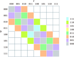
(b)

Figure S.2: Cases for the lower and upper bounds of the number of non-zero elements qq for n=3n=3 qubits and k=2k=2 bandwidth. (a) Lower-bound case q=mq=m. (b) Upper-bound case q=2n(2k+1)k(k+1)q=2^{n}(2k+1)-k(k+1). Components of the same color can be simultaneously evaluated by one measurement operator using the XBM method. The color range is defined by l=bcl=b\oplus c, where bb and cc are the row and column indices of AA.

The worst case for the variance when using the XBM method is q=m=2((nlog2k)k+2log2k)2k(1+nlog2k)q=m=2((n-\lceil\log_{2}k\rceil)k+2^{\lceil\log_{2}k\rceil})\approx 2k(1+n-\log_{2}k). In this case,

m2q={O(nc+1)whenk=O(nc)O(2n)whenk=O(2n).\displaystyle\frac{m^{2}}{q}=\left\{\begin{array}[]{ll}\displaystyle{O(n^{c+1})}&{\rm when}\ \ \ k=O(n^{c})\\[14.22636pt] O(2^{n})&{\rm when}\ \ \ k=O(2^{n})\end{array}\right..

Meanwhile, when q=2n(2k+1)k(k+1)=O(k2n)q=2^{n}(2k+1)-k(k+1)=O(k2^{n}),

m2q={O(nc+12n)whenk=O(nc)O(1)whenk=O(2n).\displaystyle\frac{m^{2}}{q}=\left\{\begin{array}[]{ll}\displaystyle{O\Bigg(\frac{n^{c+1}}{2^{n}}\Bigg)}&{\rm when}\ \ \ k=O(n^{c})\\[14.22636pt] O(1)&{\rm when}\ \ \ k=O(2^{n})\end{array}\right..

In summary,

Varp[a^]XBM={O(nc+1tr(A2))whenk=O(nc)andq=O(m)O(2ntr(A2))whenk=O(2n)andq=O(m)O(nc+12ntr(A2))whenk=O(nc)andq=O(k2n)O(tr(A2))whenk=O(2n)andq=O(k2n).\displaystyle{\color[rgb]{0,0,0}{\rm Var}_{p}\big[\hat{a}\big]_{\rm XBM}}=\left\{\begin{array}[]{ll}O\big(n^{c+1}\,{\rm tr}(A^{2})\big)&{\rm when}\ \ \ k=O(n^{c})\ \ \ {\rm and}\ \ \ q=O(m)\\[14.22636pt] O\big(2^{n}\,{\rm tr}(A^{2})\big)&{\rm when}\ \ \ k=O(2^{n})\ \ \ {\rm and}\ \ \ q=O(m)\\[14.22636pt] \displaystyle{O\Bigg(\frac{n^{c+1}}{2^{n}}\,{\rm tr}(A^{2})\Bigg)}&{\rm when}\ \ \ k=O(n^{c})\ \ \ {\rm and}\ \ \ q=O(k2^{n})\\[14.22636pt] O\big(\,{\rm tr}(A^{2})\big)&{\rm when}\ \ \ k=O(2^{n})\ \ \ {\rm and}\ \ \ q=O(k2^{n})\end{array}\right..

When q=O(m)q=O(m), which is the case shown in Fig. S.2(a), the variance associated with the XBM is worse than that associated with the classical shadow (Eqs. (C.2)1 and (C.2)2). However, when q=O(k2n)q=O(k2^{n}), which is the case shown in Fig. S.2(b), the variance associated with the XBM is at least of the same order as that associated with the classical shadow (Eqs. (C.2)3 and (C.2)4). In particular, when k=O(nc)k=O(n^{c}) and q=O(k2n)q=O(k2^{n}), which is the case that AA is a matrix with a narrow bandwidth whose non-zero elements are densely filled in the band, the variance associated with the XBM is exponentially tighter than that associated with the classical shadow (Eqs. (C.2)3). Such AA frequently appear as the global stiffness matrix in the finite element method as mentioned in the introduction of the main body.

Appendix D Classical Shadow with XBM

The XBM method is closely related to the classical shadow [31]. Let ρ\rho, 𝒰\mathcal{U} and \mathcal{M} be an arbitrary density matrix, unitary ensemble, and quantum channel, respectively. These are defined as

𝒰:={Ms(l)}l𝒮(A),s{Re,Im}\displaystyle\mathcal{U}:=\{M^{(l)}_{s}\}_{l\in\mathcal{S}(A),s\in\{{\rm Re},{\rm Im}\}} (S.92)

and

(ρ)\displaystyle\mathcal{M}(\rho) :=𝔼UP𝒰,bb|ρ|b[U|bb|U]\displaystyle:=\mathbb{E}_{U\sim{\rm P}_{\mathcal{U}},\,b\sim\langle b|\rho|b\rangle}\big[U^{\dagger}|b\rangle\langle b|U\big]
=b[p(l=0n)b|ρ|b|bb|+l𝒮(A){0n}s{Re,Im}p(l,s)b|Ms(l)ρMs(l)|bMs(l)|bb|Ms(l)],\displaystyle=\sum_{b}\Bigg[p(l=0^{n})\langle b|\rho|b\rangle|b\rangle\langle b|+\sum_{l\in\mathcal{S}(A){\color[rgb]{0,0,0}\setminus\{0^{n}\}}}\sum_{s\in\{{\rm Re},{\rm Im}\}}p(l,s)\langle b|M^{(l)}_{s}\rho M^{(l)\dagger}_{s}|b\rangle M^{(l)\dagger}_{s}|b\rangle\langle b|M^{(l)}_{s}\Bigg], (S.93)

respectively, where P𝒰{\rm P}_{\mathcal{U}} is a probability distribution over 𝒰\mathcal{U}. A classical shadow, ρ^:=1(U|bb|U)\hat{\rho}:=\mathcal{M}^{-1}\big(U^{\dagger}|b\rangle\langle b|U\big), UP𝒰U\sim{\rm P}_{\mathcal{U}}, bb|ρ|bb\sim\langle b|\rho|b\rangle, associated with the XBM method is expressed as

ρ^(l,s,b)\displaystyle\hat{\rho}(l,s,b) ={|bb|p(l=0n)forl=0n(1)w|cb|+|bc|2p(l,s=Re)forl0nands=Rei(1)w|cb||bc|2p(l,s=Im)forl0nands=Im\displaystyle=\left\{\begin{array}[]{ll}\displaystyle{\frac{|b\rangle\langle b|}{p(l=0^{n})}}&{\rm for}\ \ \ l=0^{n}\\[14.22636pt] \displaystyle{(-1)^{w}\frac{|c^{\prime}\rangle\langle b^{\prime}|+|b^{\prime}\rangle\langle c^{\prime}|}{2p(l,s={\rm Re})}}&{\rm for}\ \ \ l\neq 0^{n}\ \ \ {\rm and}\ \ \ s={\rm Re}\\[14.22636pt] \displaystyle{{\rm i}(-1)^{w}\frac{|c^{\prime}\rangle\langle b^{\prime}|-|b^{\prime}\rangle\langle c^{\prime}|}{2p(l,s={\rm Im})}}&{\rm for}\ \ \ l\neq 0^{n}\ \ \ {\rm and}\ \ \ s={\rm Im}\end{array}\right.

where (b,c,w)(b^{\prime},c^{\prime},w) are defined in Table 1. The above can be easily derived by replacing AbcA_{bc} with |cb||c\rangle\langle b| because |ψψ|=b,c|cb|ψ|bc|ψ|\psi\rangle\langle\psi|=\sum_{b,c}|c\rangle\langle b|\langle\psi|b\rangle\langle c|\psi\rangle takes the same form as Eq. (1). The simple choice for the operator selecting model is

p(l=0n)=p(l0n,s)=12n+11\displaystyle p(l=0^{n})=p(l\neq 0^{n},s)=\frac{1}{2^{n+1}-1} (S.97)

where 2n+112^{n+1}-1 is the number of unique circuits used to evaluate the expectation value of the dense 2n×2n2^{n}\times 2^{n} matrix. The classical shadow associated with the XBM method satisfies

𝔼l,s,bp(l,s,b)[ρ^(l,s,b)]=ρ\displaystyle\mathbb{E}_{l,s,b\sim p(l,s,b)}[\hat{\rho}(l,s,b)]=\rho (S.98)

and

tr(Aρ^(l,s,b))=a(l,s,b)\displaystyle{\rm tr}(A\hat{\rho}(l,s,b))=a(l,s,b) (S.99)

where a(l,s,b)a(l,s,b) is defined in Eq. (A.4). There is a low requirement of the classical memory to store the classical shadow associated with the XBM method. That is, only the indices {(l,s)}\{(l,s)\} and bit strings measured {b}\{b\} need to be stored.

The measurement operators associated with the XBM method are Clifford circuits, which consist of CNOT, Hadamard and phase gates, and therefore the XBM can be seen as the classical shadow with the random Clifford measurement whose unitary ensemble is a subset of Clifford group Cl(2n){\rm Cl}(2^{n}) (Eq. (S.92)), and the unitary is selected with probability p(l,s)p(l,s) that can be modeled to reduce the variance. From this point of view, our conclusion can be restated that by using an unitary ensemble Eq. (S.92) and appropriate operator selecting model, the expectation value can be evaluated computationally more efficiently than by using random Clifford measurements in a specific condition. Concretely,

  1. 1.

    the number of two-qubit entangling gates in each measurement operator is reduced from O(n2/log(n))O(n^{2}/\log(n)) to O(n)O(n) and

  2. 2.

    the variance reduces from O(tr(A2))O({\rm tr}(A^{2})) to O((nc+1/2n)tr(A2))O((n^{c+1}/2^{n}){\rm tr}(A^{2})) when non-zero elements of AA are densely filled in the bandwidth kk.

Appendix E Proofs

E.1 Colored Matrix


Figure S.3: Schematic illustration of the colored matrix in the case of the three-qubit system. The (b,c)(b,c) component is colored with the bcb\oplus c th color. Components of the same color can be simultaneously measured using the XBM method.

In proving theorems 2 and 3, we introduce a colored matrix (see Fig. S.3) as a visual reference. In the colored matrix, the (b,c)(b,c) component of AA is positioned on the bb th row and cc th column, and each component is colored with the bcb\oplus c th color. Components of the same color are simultaneously measurable using the XBM method. Hence, the number of colors with a non-zero element value is the same as the number of unique circuits used in evaluating ψ0|A|ψ1\big<\psi_{0}\big|A\big|\psi_{1}\big>.

E.2 Proof of Theorem 2

(a)

(b)

(c)
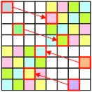
(d)
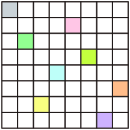
(e)
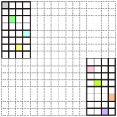
(f)
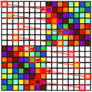
(g)
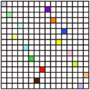
(h)
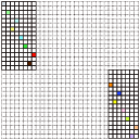
(i)

Figure S.4: Step-by-step algorithm for making a 1-sparse matrix including all colors: (a) the same illustration as in Fig. S.3 for n=2n=2; (b) in the first step, manually obtain a 1-sparse matrix for n=2n=2 including all colors; (c) split the matrix (b) in half and move the halves to the top-left and bottom-right; (d) fill the top-right and bottom-left color, copy the patterns from the top-left and bottom right to the top-right and bottom-left, respectively, and delete the unmarked square’s color; (e) 1-sparse matrix for n=3n=3 including all colors; (g)-(i) repeat (c) to (f) until the matrix has the desired size.

We show that there exists an algorithm that produces a 1-sparse matrix including all colors in the colored matrix defined in Sec. E.1. First, for the two-qubit system, a 1-sparse matrix including all four colors is found manually (Fig. S.4(a) and (b)). Next, a 22×222^{2}\times 2^{2} matrix is split in half and the halves are moved to the top-left and right-bottom of a 23×232^{3}\times 2^{3} matrix as in Fig. S.4(c). The colored patterns are then copied to the top-right and bottom-left as in Fig. S.4(d). Repeating this procedure as in Fig. S.4(e) to (i), a 1-sparse matrix including all colors is obtained for any size 2n×2n2^{n}\times 2^{n}.

\Box

E.3 Proof of Theorem 3


Figure S.5: Schematic illustration of the number of colors of the colored matrix for n=1,2,3,4n=1,2,3,4.

Figure S.6: Schematic illustration of matrix bi(j)b^{(j)}_{i} where the horizontal and vertical correspond to indices ii and jj, respectively. A filled square indicates an entry of 11 whereas a blank indicates an entry of 00. The number of entries included in the n×kn\times k square is equal to j=1ni=1kbi(j)\sum^{n}_{j=1}\sum^{k}_{i=1}b^{(j)}_{i}, which can be decomposed into the red and green square corresponding to j=1log2k2j1\sum^{\lceil\log_{2}k\rceil}_{j=1}2^{j-1} and (nlog2k)k(n-\lceil\log_{2}k\rceil)k, respectively.

The number of colors in a colored matrix of bandwidth kk, which we denote by Nk(n)N^{(n)}_{k}, is counted as in Fig. S.5. From Fig. S.5, Nk(n)N^{(n)}_{k} can be written as

Nk(n)=1+i=1k(ai(n)+bi(n))\displaystyle N^{(n)}_{k}=1+\sum^{k}_{i=1}\Big(a^{(n)}_{i}+b^{(n)}_{i}\Big) (S.100)

where

ai(1)=0,bi(n)={11i2n10else,ai(n)=ai(n1)+bi(n1).\displaystyle a^{(1)}_{i}=0,\hskip 14.22636ptb^{(n)}_{i}=\left\{\begin{array}[]{ll}1&1\leq i\leq 2^{n-1}\\ 0&{\rm else}\end{array}\right.,\hskip 14.22636pta^{(n)}_{i}=a^{(n-1)}_{i}+b^{(n-1)}_{i}.

Solving this recurrence relation, we obtain

Nk(n)=1+j=1ni=1kbi(j)=1+(nlog2k)k+j=1log2k2j1=(nr)k+2r,\displaystyle N^{(n)}_{k}=1+\sum^{n}_{j=1}\sum^{k}_{i=1}b^{(j)}_{i}=1+(n-\lceil\log_{2}k\rceil)k+\sum^{\lceil\log_{2}k\rceil}_{j=1}2^{j-1}=(n-r)k+2^{r}, (S.103)

where r:=log2kr:=\lceil\log_{2}k\rceil (see Fig. S.6).

When both real and imaginary parts of φ|bc|φ\big<\varphi\big|b\big>\big<c\big|\varphi\big> are required, the number of unique circuits is doubled. Hence, the upper bound of the number of unique circuits is 2((nr)k+2r)2((n-r)k+2^{r}). When evaluating ψ0|A|ψ1=φ|A|φ\langle\psi_{0}|A^{\prime}|\psi_{1}\rangle=\langle\varphi|A|\varphi\rangle with |ψ0=|ψ1|\psi_{0}\rangle=|\psi_{1}\rangle, the matrix AA can have non-zero diagonal components. Considering that Im(φ|bb|φ)=Im(|b|φ|2)=0{\rm Im}\big(\big<\varphi\big|b\big>\big<b\big|\varphi\big>\big)={\rm Im}\big(|\big<b\big|\varphi\big>|^{2}\big)=0, the upper bound of the number of unique circuits can be reduced to 2((nr)k+2r)12((n-r)k+2^{r})-1 in this case.

\Box

E.4 Naïve Pauli measurements

When Abc0A_{bc}\neq 0, Tr(A𝐏){\rm Tr}\big(A^{\dagger}{\bf P}\big) takes a non-zero value where 𝐏:=P(bc)n1P(bc)n2P(bc)0{\bf P}:=P_{(b\oplus c)_{n-1}}\otimes P_{(b\oplus c)_{n-2}}\otimes\cdots\otimes P_{(b\oplus c)_{0}}, P0{I,Z}P_{0}\in\{I,Z\}, P1{X,Y}P_{1}\in\{X,Y\}, and II, XX, YY and ZZ are the Pauli matrices. Therefore, for each distinct bcb\oplus c such that Abc0A_{bc}\neq 0, 2n2^{n} Pauli strings are required to express ψ0|A|ψ0=𝐏(Tr(A𝐏)/2n)ψ0|𝐏|ψ0\big<\psi_{0}\big|A\big|\psi_{0}\big>=\sum_{\bf P}\Big({\rm Tr}\big(A^{\dagger}{\bf P}\big)/2^{n}\Big)\big<\psi_{0}\big|{\bf P}\big|\psi_{0}\big>. The number of distinct bcb\oplus c is the same as the number of colors in the colored matrix defined in Sec. E.1, and the number of unique Pauli strings required to express ψ0|A|ψ0\big<\psi_{0}\big|A\big|\psi_{0}\big> is therefore 2n((nr)k+2r)2^{n}((n-r)k+2^{r}). In the case that ψ0|A|ψ1\big<\psi_{0}\big|A\big|\psi_{1}\big>, 𝐏:=PnP(bc)n1P(bc)n2P(bc)0{\bf P}:=P_{n}\otimes P_{(b\oplus c)_{n-1}}\otimes P_{(b\oplus c)_{n-2}}\otimes\cdots\otimes P_{(b\oplus c)_{0}} is used instead where Pn{X,Y}P_{n}\in\{X,Y\} and the number of unique Pauli strings required to express ψ0|A|ψ1\big<\psi_{0}\big|A\big|\psi_{1}\big> is therefore 2n+1((nr)k+2r)2^{n+1}((n-r)k+2^{r}).

E.5 Evaluating Pauli strings by XBM

Consider evaluating an expectation value of one given Pauli string using the XBM method. Let σn1σn2σ1σ0\sigma_{n-1}\sigma_{n-2}\cdots\sigma_{1}\sigma_{0} be a Pauli string where σi{I,X,Y,Z}\sigma_{i}\in\{I,X,Y,Z\}. Converting this Pauli string into a row-column basis gives a matrix AA where Ab,bp0A_{b,b\oplus p}\neq 0 for all b=0,1,,2n1b=0,1,\cdots,2^{n}-1 and pp is a bit string defined as

pi\displaystyle p_{i} :={0ifσi{I,Z}1ifσi{X,Y}.\displaystyle:=\left\{\begin{array}[]{ll}0&{\rm if}\ \ \ \sigma_{i}\in\{I,Z\}\\[14.22636pt] 1&{\rm if}\ \ \ \sigma_{i}\in\{X,Y\}\end{array}\right..

The non-zero elements of AA are simultaneously measurable using the XBM method because the XBM method groups all AbcA_{bc} that satisfy bc=bcb\oplus c=b^{\prime}\oplus c^{\prime}, and b(bp)=pb\oplus(b\oplus p)=p. For example, consider XIYYZXIYYZ. In this case, p=10110p=10110 and non-zero elements of AA are A00000,10110,A00001,10111,,A11111,01001A_{00000,10110},A_{00001,10111},\cdots,A_{11111,01001}. All components of such AA are simultaneously measurable using the XBM method because 0000010110=0000110111==1111101001=10110=p00000\oplus 10110=00001\oplus 10111=\cdots=11111\oplus 01001=10110=p. Therefore, the number of unique circuits to evaluate φ|XIYYZ|φ\big<\varphi\big|XIYYZ\big|\varphi\big> using the XBM method is two (corresponding to the real and imaginary parts).