Balancing Value Underestimation and Overestimation with Realistic Actor-Critic

Abstract

Model-free deep reinforcement learning (RL) has been successfully applied to challenging continuous control domains. However, poor sample efficiency prevents these methods from being widely used in real-world domains. This paper introduces a novel model-free algorithm, Realistic Actor-Critic(RAC), which can be incorporated with any off-policy RL algorithms to improve sample efficiency. RAC employs Universal Value Function Approximators (UVFA) to simultaneously learn a policy family with the same neural network, each with different trade-offs between underestimation and overestimation. To learn such policies, we introduce uncertainty punished Q-learning, which uses uncertainty from the ensembling of multiple critics to build various confidence-bounds of Q-function. We evaluate RAC on the MuJoCo benchmark, achieving 10x sample efficiency and 25% performance improvement on the most challenging Humanoid environment compared to SAC.

1 Introduction

Sample efficiency is one of the main challenges that prevent reinforcement learning(RL) applying to real-world systems [13, 43]. Recently, in continuous control domains, model-free off-policy reinforcement learning(RL) method has achieved a comparable sample efficiency to model-based methods by training accurate value approximations with a high Update-To-Data (UTD) ratio [10]. Quality of value approximation is a key for sample efficiency, stability and final performance as policy optimization relies on gradients of Q-functions to provide the direction of the policy update.

Overestimation bias and accumulation of function approximation errors in temporal difference methods [44, 38, 15] are some of the main factors that plague value approximation. Undesirable overestimation bias may lead to sub-optimal policy updates and divergent behavior.

One way to address above issues is using ensemble methods [28, 15, 29, 10, 27] to introduce underestimation bias which does not tend to be propagated during learning, as actions with low value estimates are avoided by the policy. However, underestimation bias may harm exploration by causing a pessimistic underexploration problem [11]. Both under- and overestimation bias may improve learning performance, depending on the environment [28]. To overcome this problem, carefully adjusted hyperparameters are needed to trade off between under- and overestimation.

In this paper, we propose Realistic Actor-Critic (RAC) to address this under-overestimation trade-off, whose main idea is to learn together diverse policies with respect to various confidence-bounds of Q-functions in the same network. In such a way, policies guided by upper confidence bounds (UCB) generate effective exploratory behaviors without falling in pessimistic underexploration, while other policies benefit from lower-confidence bounds(LCB) to control overestimation bias to provide consistency and stable convergence. We propose to jointly learn such family of policies parameterized with the Universal Value Function Approximators (UVFA) [41]. The best policy can be found by evaluating the learned policies at the evaluation phase. The learning process can be considered as a set of auxiliary tasks [5, 31] that help build shared state representations and sills.

However, learning such policies with diverse behaviors in a single network is challenging. We introduce uncertainty punished Q-learning(UPQ), which calculates uncertainty as punishment to correct value estimations. UPQ provides fine-granular overestimation control to make value approximation smoothly shifts from upper bounds to lower bounds. With UPQ, RAC incorporates various bounds of Q-function into a critic with UVFA to update policies that change smoothly. We propose to learn an ensemble of multiple critics that produces well-calibrated uncertainty estimations (i.e., standard deviation) on unseen samples [29, 36, 2]. We show empirically that RAC controls the std and the mean of value estimate bias to close to zero for most of the training. Benefit from well value estimation, critics are trained with a high UTD ratio to improve sample efficiency significantly.

Empirically, we evaluate RAC combined with SAC [17] and TD3 [15] in continuous control benchmarks (OpenAI Gym [7], MuJoCo [45]). Numerical results suggest RAC outperforms the current state of the art algorithms (MBPO [20], REDQ [10] and TQC [27]). RAC demonstrates 10x sample efficiency and 25% performance improvement on the most challenging Humanoid environment compared to SAC. We perform ablations and isolate the effect of the main components of RAC on performance. Moreover, we perform hyperparameter ablations and demonstrate that RAC is stable in practice.

2 Related work

Underestimation and overestimation of Q-function. The maximization update rule in Q-learning has been shown to suffer from overestimation bias which will seriously hinder learning [44].

Minimization of a value ensemble is a common method to deal with overestimation bias. Clipped double Q-learning (CDQ) [15] takes the minimum value between a pair of critics to limit overestimation. SAC [17] then combined CDQ with entropy maximization to get impressive performance in continuous control tasks. Maxmin Q-learning [28] mitigated the overestimation bias by using a minimization over multiple action-value estimates. But minimize a Q-function set is unable to filter out abnormally small values which causes undesired pessimistic underexploration problem [11]. Using minimization to control overestimation is coarse and wasteful as it ignores all estimates except the minimal one [27].

REDQ [10] proposed in-target minimization which used a minimization across a random subset of Q functions from the ensemble to alleviate the above problems. REDQ [10] showed their method reduces the std of the Q-function bias to close to zero for most of the training. Truncated Quantile Critics (TQC) [27] truncates the right tail of the distributional value ensemble by dropping several of the topmost atoms to control overestimation. Weighted bellman backups [29] and uncertainty weighted actor-critic [49] prevents error propagation [26] in Q-learning by reweighing sample transitions based on uncertainty estimations from the ensembles [29] or Monte Carlo dropout [49, 42]. Different from prior works, our work does not reweight sample transitions but directly adds uncertainty estimations to punish the target value.

Lan et al. [28] showed the effect of underestimation bias on learning efficiency is environment-dependent. It may be hard to choose the right parameters to balance under- and overestimation for completely different environments. Our work proposed to solve this problem by learning an optimistic and pessimistic policy family.

Ensemble methods. In deep learning, ensemble methods often used to solve the two key issues, uncertainty estimations [47, 1] and out-of-distribution robustness [18, 14, 48]. In reinforcement learning, using ensemble to enhance value function estimation was widely studied, such as, averaging a Q-ensemble [3, 37], bootstrapped actor-critic architecture [22, 50], calculate uncertainty to reweight sample transitions [29], minimization over ensemble estimates [28, 10] and update the actor with a value ensemble [27, 10].

A high-level policy can be distilled from a policy ensemble  [8, 4] by density-based selection [40], selection through elimination [40], choosing action that max all Q-functions  [29, 34, 21], Thompson Sampling [34] and sliding-window UCBs [4]. Leveraging uncertainty estimations of the ensemble,  [33, 22, 50] simulated training different policies with a multi-head architecture independently to generate diverse exploratory behaviors.

Ensemble methods were also used to learn joint state presentation to improve sample efficiency. There were two main methods: multi-heads  [33, 22, 50, 16] and UVFA [41, 5, 4]. In this paper, we uses uncertainty estimation to reduce value overestimation bias, a simple max strategy to to get the best policy and learning joint state presentation with UVFA.

Optimistic exploration. Pessimistic initialisation [39] and learning policy that maximizes a lower-confidence bound value could suffer pessimistic underexploration problem [11]. Optimistic exploration is a promising solution to ease the above problem by applying the principle of optimism in the face of uncertainty [6]. Disagreement [36] and EMI [23] considered uncertainty as intrinsic motivation to encourage agent to explore the high uncertainty areas of the environment. Uncertainty punishment proposed in this paper can also be thought of as a special intrinsic motivation. Different with [36, 23] which usually choose the weighting $\geq 0$ to encourage exploration, UPQ using the weighting $\leq 0$ to control value bias.

SUNRISE [29] proposed an optimistic exploration that chooses the action that maximizes an upper-confidence bound (UCB) [9] of Q-functions. OAC [11] proposed an off-policy exploration strategy that is adjusted to a linear fit of UCB to the critic with the maximum KL divergence constraining between the exploration policy and the target policy.

Most importantly, our work provides a unified framework for the under-overestimation trade-off.

3 RAC

We present Realistic Actor-Critic (RAC) which can be used in conjunction with most modern off-policy actor-critic RL algorithms in principle, such as SAC [17] and TD3 [15]. For the exposition, we describe only the SAC version of RAC (RAC-SAC) in the main body. The TD3 version of RAC (RAC-TD3) follows the same principles and is fully described in Appendix A.

3.1 Problem setting and preliminaries

We consider the standard reinforcement learning notation, with states $\mathbf{s}$, actions $\mathbf{a}$, reward $r(\mathbf{s},\mathbf{a})$, and dynamics $p(\mathbf{s^{\prime}}\mid\mathbf{s},\mathbf{a})$. The discounted return $R_{t}={\textstyle\sum_{k=0}^{\infty}}\gamma^{k}r_{k}$ is the total accumulated rewards from timestep $t$, $\gamma\in[0,1]$ is a discount factor determining the priority of short-term rewards. The objective is to find the optimal policy $\pi_{\phi}(\mathbf{s}\mid\mathbf{a})$ with parameters $\phi$, which maximizes the expected return $J(\phi)=\mathbb{E}_{p_{\pi}}\left[R_{t}\right]$.

The maximum entropy objective [51] encourages the robustness to noise and exploration by maximizing a weighted objective of the reward and the policy entropy:

$$\pi^{*}=\arg\max_{\pi}\sum_{t}\mathbb{E}_{\mathbf{s}\sim p,\mathbf{a}\sim\pi}\left[r(\mathbf{s},\mathbf{a})+\alpha\mathcal{H}\left(\pi\left(\cdot\mid\mathbf{s}\right)\right)\right],$$ (1)

where $\alpha$ is the temperature parameter that can be used to determine the relative importance of entropy and reward. Soft Actor-Critic(SAC) [17] seeks to optimize the maximum entropy objective by alternating between a soft policy evaluation and a soft policy improvement. A parameterized soft Q-function $Q_{\theta}\left(\mathbf{s},\mathbf{a}\right)$ , known as the critic in actor-critic methods, is trained by minimizing the soft Bellman residual:

$$\mathcal{L}_{\tt critic}(\theta)=\mathbb{E}_{\tau\sim\mathcal{B}}[\left(Q_{\theta}(\mathbf{s},\mathbf{a})-y\right)^{2}],$$ (2)

$$y=r-\gamma\mathbb{E}_{\mathbf{a^{\prime}}\sim\pi_{\phi}}\big{[}Q_{\bar{\theta}}(\mathbf{s^{\prime}},\mathbf{a^{\prime}})-\alpha\log\pi_{\phi}(\mathbf{a^{\prime}}\mid\mathbf{s^{\prime}})\big{]},$$ (3)

where $\tau=(\mathbf{s},\mathbf{a},r,\mathbf{s^{\prime}})$ is a transition, $\mathcal{B}$ is a replay buffer, $\bar{\theta}$ are the delayed parameters which is updated by exponential moving average $\bar{\theta}\leftarrow\rho\theta+(1-\rho)\bar{\theta}$, $\rho$ is the target smoothing coefficient, $y$ is the target value.

The parameterized policy $\pi_{\phi}$ , known as the actor, is updated by minimizing the following object:

$$\mathcal{L}_{\tt actor}(\phi)=\mathbb{E}_{\mathbf{s}\sim\mathcal{B},\mathbf{a}\sim\pi_{\phi}}\left[\alpha\log\left(\pi_{\phi}\left(\mathbf{a}\mid\mathbf{s}\right)\right)-Q_{\theta}\left(\mathbf{a},\mathbf{s}\right)\right].$$ (4)

SAC uses a automate entropy adjusting mechanism to update $\alpha$ with following objective:

$$\mathcal{L}_{\tt temp}(\alpha)=\mathbb{E}_{\mathbf{s}\sim\mathcal{B},\mathbf{a}\sim\pi_{\phi}}\left[-\alpha\log\pi_{\phi}\left(\mathbf{a}\mid\mathbf{s}\right)-\alpha\overline{\mathcal{H}}\right],$$ (5)

where $\overline{\mathcal{H}}$ is the target entropy.

3.2 Uncertainty punished Q-learning

Uncertainty punished Q-learning(UPQ) is a variant of soft Bellman residual(2). The idea is to maintain an ensemble of $N$ soft Q-functions $Q_{\theta_{i}}(\mathbf{s},\mathbf{a})$, where $\theta_{i}$ denote the parameters of the $i-th$ soft Q-function, which are initialized randomly and independently for inducing an initial diversity in the models [33], but updated with the same target.

Given a transition $\tau_{t}$, UPQ consider following uncertainty punished target $y$:

$$y=r_{t}+\gamma\mathbb{E}_{\mathbf{a^{\prime}}\sim\pi_{\phi}}\left[\bar{Q}_{\bar{\theta}}(\mathbf{s^{\prime}},\mathbf{a^{\prime}})-\beta\hat{s}({Q}_{\bar{\theta}}(\mathbf{s^{\prime}},\mathbf{a^{\prime}}))-\alpha\log\pi_{\phi}\left(\mathbf{a^{\prime}}\mid\mathbf{s^{\prime}}\right)\right],$$ (6)

$$\bar{Q}_{\bar{\theta}}(\mathbf{s^{\prime}},\mathbf{a^{\prime}})=\frac{1}{N}\sum_{i=1}^{N}Q_{\bar{\theta}_{i}}(\mathbf{s^{\prime}},\mathbf{a^{\prime}}),$$ (7)

$$\hat{s}({Q}_{\bar{\theta}}(\mathbf{s^{\prime}},\mathbf{a^{\prime}}))=\sqrt{\frac{1}{N-1}\sum_{i=1}^{N}\left[Q_{\bar{\theta}_{i}}(\mathbf{s^{\prime}},\mathbf{a^{\prime}})-\bar{Q}_{\bar{\theta}}(\mathbf{s^{\prime}},\mathbf{a^{\prime}})\right]^{2}},$$ (8)

where $\bar{Q}_{\bar{\theta}}(\mathbf{s},\mathbf{a})$ is the sample mean of target Q-functions, $\hat{s}({Q}_{\bar{\theta}}(\mathbf{s},\mathbf{a}))$ is the sample standard deviation of target Q-functions with bessel’s correction [46]. UPQ uses $\hat{s}({Q}_{\bar{\theta}}(\mathbf{s},\mathbf{a}))$ as uncertainty estimation to punish value estimation. $\beta\geq 0$ is the weighting of the punishment. Note that we do not propagate gradient through the uncertainty $\hat{s}({Q}_{\bar{\theta}}(\mathbf{s},\mathbf{a}))$.

We write $Q_{\mathbf{s}\mathbf{a}}^{i}$ instead of $Q_{\theta_{i}}(\mathbf{s},\mathbf{a})$, $Q_{\mathbf{s^{\prime}}\mathbf{a^{\prime}}}^{i}$ instead of $Q_{\theta_{i}}(\mathbf{s^{\prime}},\mathbf{a^{\prime}})$ for compactness. Assuming each Q-function has random approximation error $e_{\mathbf{s}\mathbf{a}}^{i}$ [44, 28, 10] which is a random variable belonging to some distribution

$$Q_{\mathbf{s}\mathbf{a}}^{i}=Q_{\mathbf{s}\mathbf{a}}^{*}+e_{\mathbf{s}\mathbf{a}}^{i},$$ (9)

where $Q_{\mathbf{s}\mathbf{a}}^{*}$ is the ground truth of Q-functions. $M$ is the number of actions applicable at state $\mathbf{s^{\prime}}$. Define the estimation bias $Z_{MN}$ for a transition $\tau_{t}$ to be

$$Z_{MN} \stackrel{{\scriptstyle\text{ def }}}{{=}}\left[r+\gamma\max_{\mathbf{a}^{\prime}}(Q_{\mathbf{s}^{\prime}\mathbf{a}^{\prime}}^{mean}-\beta Q_{\mathbf{s}^{\prime}\mathbf{a}^{\prime}}^{std})\right]-\left(r+\gamma\max_{\mathbf{a}^{\prime}}Q_{\mathbf{s}^{\prime}\mathbf{a}^{\prime}}^{*}\right)$$ (10)

$$=\gamma\left[\max_{\mathbf{a}^{\prime}}(Q_{\mathbf{s}^{\prime}\mathbf{a}^{\prime}}^{mean}-\beta Q_{\mathbf{s}^{\prime}\mathbf{a}^{\prime}}^{std})-\max_{\mathbf{a}^{\prime}}Q_{\mathbf{s}^{\prime}\mathbf{a}^{\prime}}^{*}\right],$$ (11)

where

$$Q_{\mathbf{s}^{\prime}\mathbf{a}^{\prime}}^{mean} \approx\frac{1}{N}\sum_{i=1}^{N}Q_{\mathbf{s^{\prime}}\mathbf{a^{\prime}}}^{i}=\frac{1}{N}\sum_{i=1}^{N}(Q_{\mathbf{s^{\prime}}\mathbf{a^{\prime}}}^{*}+e_{\mathbf{s^{\prime}}\mathbf{a^{\prime}}}^{i})=Q_{\mathbf{s^{\prime}}\mathbf{a^{\prime}}}^{*}+\frac{1}{N}\sum_{i=1}^{N}e_{\mathbf{s^{\prime}}\mathbf{a^{\prime}}}^{i}=Q_{\mathbf{s^{\prime}}\mathbf{a^{\prime}}}^{*}+\bar{e}_{\mathbf{s^{\prime}}\mathbf{a^{\prime}}},$$ (12)

$$Q_{\mathbf{s}^{\prime}\mathbf{a}^{\prime}}^{std} \approx\sqrt{\frac{1}{N-1}\sum_{i=1}^{N}\left(Q_{\mathbf{s}^{\prime}\mathbf{a}^{\prime}}^{i}-Q_{\mathbf{s}^{\prime}\mathbf{a}^{\prime}}^{mean}\right)^{2}}=\sqrt{\frac{1}{N-1}\sum_{i=1}^{N}\left(Q_{\mathbf{s^{\prime}}\mathbf{a^{\prime}}}^{*}+e_{\mathbf{s^{\prime}}\mathbf{a^{\prime}}}^{i}-Q_{\mathbf{s^{\prime}}\mathbf{a^{\prime}}}^{*}+\bar{e}_{\mathbf{s^{\prime}}\mathbf{a^{\prime}}}\right)^{2}}$$ (13)

$$=\sqrt{\frac{1}{N-1}\sum_{i=1}^{N}\left(e_{\mathbf{s^{\prime}}\mathbf{a^{\prime}}}^{i}-\bar{e}_{\mathbf{s^{\prime}}\mathbf{a^{\prime}}}\right)^{2}}=\hat{s}(e_{\mathbf{s^{\prime}}\mathbf{a^{\prime}}}).$$ (14)

Then

$$Z_{MN}\approx\gamma\left[\max_{\mathbf{a}^{\prime}}(Q_{\mathbf{s^{\prime}}\mathbf{a^{\prime}}}^{*}+\bar{e}_{\mathbf{s^{\prime}}\mathbf{a^{\prime}}}-\beta\hat{s}(e_{\mathbf{s^{\prime}}\mathbf{a^{\prime}}}))-\max_{\mathbf{a}^{\prime}}Q_{\mathbf{s}^{\prime}\mathbf{a}^{\prime}}^{*}\right].$$ (15)

If one could choose $\beta=\frac{\bar{e}_{\mathbf{s^{\prime}}\mathbf{a^{\prime}}}}{\hat{s}(e_{\mathbf{s^{\prime}}\mathbf{a^{\prime}}})}$, $Q_{\mathbf{s}\mathbf{a}}^{i}$ will be resumed to $Q_{\mathbf{s}\mathbf{a}}^{*}$, then $Z_{MN}$ can be reduced to near 0. However, it’s hard to adjust a suitable constant $\beta$ for various state-action pairs actually. We develop vanilla RAC which uses a constant $\beta$ in section 4.3 to research this problem.

Shifting smoothly between higher and lower bounds. For $\beta$ = 0, the update is simple average Q-learning which causes overestimation bias [10]. As $\beta$ increasing, increasingly penalties $Q_{\mathbf{s}^{\prime}\mathbf{a}^{\prime}}^{std}$ decrease $E[Z_{MN}]$ gradually, and encourage Q-functions transit smoothly from higher-bounds to lower-bounds.

Stable target estimation. Standard deviation and mean of target Q-functions used in UPQ are not sensitive to function approximation errors resulting a stable target estimation.

3.3 Realistic actor-critic agent

Algorithm 1 RAC: SAC version

1:Initialize actor network $\phi$, $N$ critic networks $\theta_{i},i=1,\ldots,N$, temperature network $\psi$, empty replay buffer $\mathcal{B}$, target network $\bar{\theta_{i}}\longleftarrow\theta_{i}$, for $i=1,2,\ldots,N$, uniform distribution $U_{1}$ and $U_{2}$

2:for each iteration do

3:     execute an action $a\sim\pi_{\phi}\left(\cdot\mid s,\beta\right),\beta\sim U_{2}$. Observe reward $r_{t}$, new state $s^{\prime}$

4:     Store transition tuple $\mathcal{B}\leftarrow\mathcal{B}\cup\left\{\left(s,a,r_{t},s^{\prime}\right)\right\}$

5:     for $G$ updates do

6:         Sample random minibatch $\{\tau_{j}\}_{j=1}^{B}\sim\mathcal{B}$, $\{\beta_{m}\}_{m=1}^{B}\sim U_{1}$

7:         Compute the Q target (18)

8:         for $i=1,\ldots,N$ do

9:              Update $\theta_{i}$ by minimize $\mathcal{L}^{\tt RAC}_{\tt critic}$ (17)

10:              Update target networks with $\bar{\theta_{i}}\leftarrow\rho\bar{\theta_{i}}+(1-\rho)\theta_{i}$

11:         end for

12:     end for

13:     Update actor parameters $\phi$ by minimize $\mathcal{L}^{\tt RAC-SAC}_{\tt actor}$ (19)

14:     Update temperature parameters $\psi$ by minimize $\mathcal{L}^{\tt RAC}_{\tt temp}$ (16)

15:end for

We now demonstrate how to use UPQ to incorporate various bounds of value approximations into a full agent that maintains diverse policies, each with a different under-overestimation trade-off. The pseudocode for RAC-SAC is shown in Algorithm 1.

RAC use a UVFA [41] to extend the critic and actor as $Q_{\theta_{i}}(\mathbf{s},\mathbf{a},\beta)$ and $\pi_{\phi}\left(\cdot\mid\mathbf{s^{\prime}},\beta\right)$, $U_{1}$ is a uniform traning distribution $\mathcal{U}[0,a]$, $a$ a is a positive real number, $\beta\sim U_{1}$ that generates various bounds of value approximations.

An independent temperature network $\alpha_{\psi}$ parameterized by $\psi$ is used to accurately adjust the temperature with respect to $\beta$, which can improve the performance of RAC. Then the objective (5) becomes:

$$\mathcal{L}^{\tt RAC}_{\tt temp}(\psi)=\mathbb{E}_{\mathbf{s}\sim\mathcal{B},\mathbf{a}\sim\pi_{\phi},\beta\sim U_{1}}\left[-\alpha_{\psi}(\beta)\log\pi_{\phi}\left(\mathbf{a}\mid\mathbf{s},\beta\right)-\alpha_{\psi}(\beta)\overline{\mathcal{H}}\right].$$ (16)

The extended Q-ensemble use UPQ to simultaneously approximate a soft Q-function family:

$$\mathcal{L}^{\tt RAC}_{\tt critic}(\theta_{i})=\mathbb{E}_{\tau\sim\mathcal{B},\beta\sim U_{1}}[\left(Q_{\theta_{i}}(\mathbf{s},\mathbf{a},\beta)-y\right)^{2}],$$ (17)

$$y=r+\gamma\mathbb{E}_{\mathbf{a^{\prime}}\sim\pi_{\phi}}[\bar{Q}_{\bar{\theta}}(\mathbf{s^{\prime}},\mathbf{a^{\prime}},\beta)-\beta\hat{s}({Q}_{\bar{\theta}}(\mathbf{s^{\prime}},\mathbf{a^{\prime}},\beta))-\alpha_{\psi}(\beta)\log\pi_{\phi}(\mathbf{a^{\prime}}\mid\mathbf{s^{\prime}},\beta)],$$ (18)

where $\bar{Q}_{\bar{\theta}}(\mathbf{s},\mathbf{a},\beta)$ is the sample mean of target Q-functions, $\hat{s}({Q}_{\bar{\theta}}(\mathbf{s},\mathbf{a},\beta))$ is the corrected sample standard deviation of target Q-functions.

The extended policy $\pi_{\phi}$ is updated by minimizing the following object:

$$\mathcal{L}^{\tt RAC-SAC}_{\tt actor}(\phi)=\mathbb{E}_{\mathbf{s}\sim\mathcal{B},\beta\sim U_{1}}\left[\mathbb{E}_{\mathbf{a}\sim\pi_{\phi}}\left[\alpha_{\psi}(\beta)\log\left(\pi_{\phi}\left(\mathbf{a}\mid\mathbf{s},\beta\right)\right)-\bar{Q}_{\theta}\left(\mathbf{a},\mathbf{s},\beta\right)\right]\right],$$ (19)

where $\bar{Q}_{\theta}\left(\mathbf{a},\mathbf{s},\beta\right)$ is the sample mean of Q-functions.

Note that, we find that apply different samples, which are generated by binary masks from the Bernoulli distribution [29, 33], to train each Q-function won’t improve RAC performance in our experiments, therefore RAC does not apply this method.

RAC circumvents direct adjustment of $\beta$. RAC leaners with a distribution of $\beta$ instead of a constant $\beta$. one could evaluate the policy family to find the best $\beta$. We employ a discrete number $H$ of values $\left\{\beta_{i}\right\}_{i=1}^{H}$ (see details in Appendix  A.2) to implement a distributed evaluation for computational efficiency, and apply the max strategy to get best $\beta$.

Optimistic exploration. When interacting with the environment, we propose to sample $\beta$ uniformly from a uniform explore distribution $U_{2}=\mathcal{U}[0,b]$,where $b<a$ is a positive real number, to get optimistic exploratory behaviors to avoid pessimistic underexploration [11]. The diversified policies with respect to different $\beta$ generate varied action sequences to visit unseen state-action pairs following the principle of optimism in the face of uncertainty [11, 29, 9].

Sample efficiency. RAC improves sample efficiency from two aspects: (1) Larger UTD ratio $G$ improves samples utilization. (2) Learning smoothly and diverse policies in the same network build a powerful representation and set of skills that can be quickly transferred to the expected policy. And we find that a smaller replay buffer capacity slightly improves the sample efficiency of RAC in section 4.4.

4 Experiments

We designed our experiments to answer the following questions:

• Can Realistic Actor-Critic outperform state-of-the-art algorithms in continuous control tasks?

• Can uncertainty punished Q-learning(UPQ) improve the quality of value approximation?

• What is the contribution of each technique in Realistic Actor-Critic?

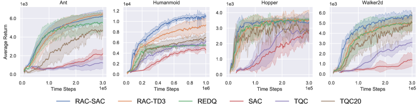
Figure 1: The learning curves on 4 Mujoco environments. The horizontal axis indicates number of time steps. The vertical axis indicates the average undiscounted return. The shaded areas denote one standard deviation.

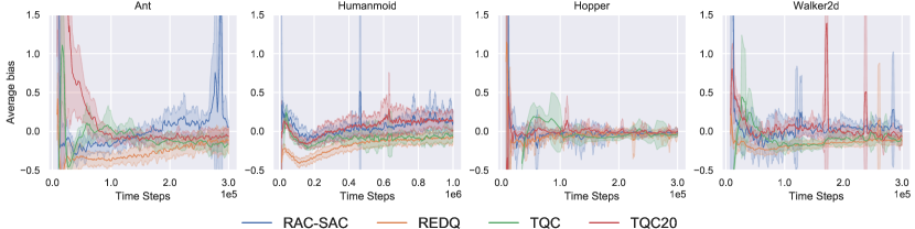
Figure 2: Mean of normalized Q bias of RAC-SAC, REDQ, TQC and TQC20 for mujoco environments.

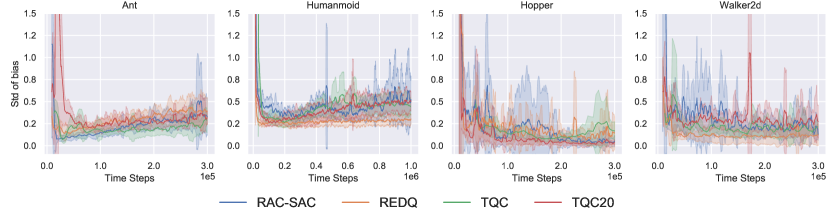
Figure 3: Std of normalized Q bias of RAC-SAC, REDQ, TQC and TQC20 for mujoco environments.

4.1 Setups

We implement RAC with SAC and TD3 as RAC-SAC and RAC-TD3(see more details in Appendix B). We compare to state-of-the-art algorithms: SAC [17], TD3 [15], MBPO [20], REDQ [10] and TQC [27] on 4 challenging continuous control tasks (Walker2d, HalfCheetah, Ant and Humanoid) from MuJoCo environments [45] in the OpenAI gym benchmark [7]. We alse implement TQC20 which is a varient of TQC with UTD $G=20$ for a fair comparison.

The time steps for training instances on Walker2d, Hopper, and Ant are $3\times 10^{5}$, and $1\times 10^{6}$ for Humanoid. All algorithms explore with a stochastic policy but use a deterministic policy for evaluation which is similar to those in SAC. We report the mean and standard deviation across 8 seeds. To analysis the value approximation quality, we calculate the mean and std of normalized values bias as main analysis indicators following REDQ [10](described in Appendix A.3). The average bias lets us know whether $Q_{\theta}$ is overestimated or underestimated, while std measures whether $Q_{\theta}$ is overfitting.

4.2 Comparative evaluation

	RAC-SAC	RAC-TD3	REDQ	MBPO	TQC20	TD3	SAC	TQC
Humanmoid	11107$\pm$475	9321$\pm$1126	5504$\pm$120	5162$\pm$350	7053$\pm$857	7014$\pm$643	7681$\pm$1118	10731$\pm$1296
Ant	6283$\pm$549	6470$\pm$165	5475$\pm$890	5281$\pm$699	4722$\pm$567	6796$\pm$277	6433$\pm$332	6402$\pm$1371
Walker	5860$\pm$440	5114$\pm$489	5034$\pm$711	4864$\pm$488	5109$\pm$696	4419$\pm$1682	5249$\pm$554	5821$\pm$457
Hopper	3421$\pm$483	3495$\pm$672	3563$\pm$94	3280$\pm$455	3208$\pm$538	3433$\pm$321	2815$\pm$585	3011$\pm$866

Table 1: Performance on OpenAI Gym. The best results are indicated in bold. Performances of SAC, TD3 and TQC are obtained with 10x samples at $6\times 10^{6}$ timesteps for Humanmoid and $3\times 10^{6}$ timesteps for other environments.

	RAC-SAC	REDQ	MBPO	TQC	TQC20	REDQ/RAC-SAC	MBPO/RAC-SAC	TQC/RAC-SAC	TQC20/RAC-SAC
Humanmoid at $2000$	63K	109K	154K	145K	147K	1.73	2.44	2.30	2.33
Humanmoid at $5000$	134K	250K	295K	445K	258K	1.87	2.20	3.32	1.93
Humanmoid at $10000$	552K	-	-	3260K	-	-	-	5.91	-
Ant at $1000$	21K	28K	62K	185K	42K	1.33	2.95	8.81	2.00
Ant at $3000$	56K	56K	152K	940K	79K	1.00	2.71	16.79	1.41
Ant at $6000$	248K	-	-	3055K	-	-	-	12.31	-
Walker at $1000$	27K	42K	54K	110K	50K	1.56	2.00	4.07	1.85
Walker at $3000$	53K	79K	86K	270K	89K	1.49	1.62	10.75	1.68
Walker at $5000$	147K	272K	-	960K	270K	1.85	-	6.53	1.84

Table 2: Sample efficiency (SE) [10, 12] is measure by the ratio of the number of samples collected when RAC and some algorithm reach the specified performance. The last 4 rows show how many times REDQ are more sample efficient than other algorithms in reaching that performance. Hopper is not in the comparison object as the performance of algorithms is almost indistinguishable.

OpenAI Gym. Figure 1 and Table 1 shows learning curves and performance comparison. RAC consistently improves the performance of SAC and TD3 across all environments and performs consistently better than other algorithms especially in Humanmoid. Table 1 shows that RAC-SAC can outperform SAC’s performance with about one-tenth of the samples. It is seen that RAC yields a much smaller variance than SAC and TQC which implies that the optimistic exploration helps the agents escape out of bad local optima.

Sample efficiency comparison. Results in table 2 show that the sampling efficiency of RAC exceeds other algorithms. Compared with TQC, RAC-SAC reaches 3000 and 6000 for Ant with 16.79x and 12.31x sample efficiency. RAC-SAC performs 1.5x better than REDQ half-way through training and 1.8x better at the end of training in Walker and Huamnmoid. The sample efficiency of TQC20 is also significantly improved compared to TQC which show that the UTD ratio is indeed a key factor to sample efficiency.

Value approximation analysis. Figure 2 and 3 presents std and mean of normalized Q bias. In Ant and humanmoid, RAC-SAC quickly suppresses overestimation at the beginning of training and reduces the std to a lower level. Different with REDQ which always keeps negative Q bias, RAC-SAC slowly moves Q bias towards from underestimation to overestimation without injuring performance. This abnormal phenomenon indicates that overestimation can still effectively improve the performance of agents in some situation which is consistent with  Lan et al. [28]’s view.

Performance of different confidence bounds. Results in Figure 4 show that Ant is not sensitive to value confidence bounds, while small changes in $\beta$ will have a huge impact on the performance of RAC-SAC at Humanmoid, Walker2d and Hopper. Figure 5 shows the best $\beta$ for different environments and time steps can be completely different, using a constant $\beta$ is unreasonable.

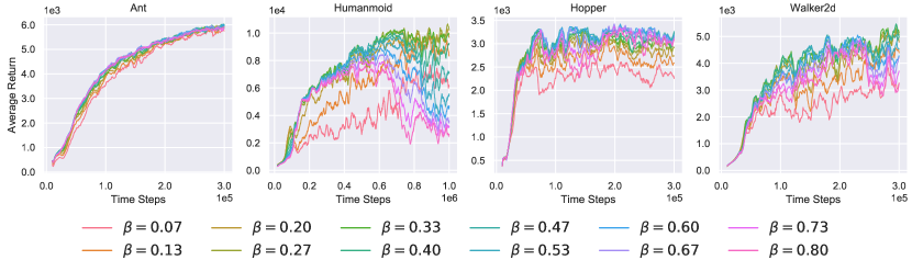
Figure 4: Performance of various value confidence bounds with respect to different $\beta$ during training for RAC-SAC.

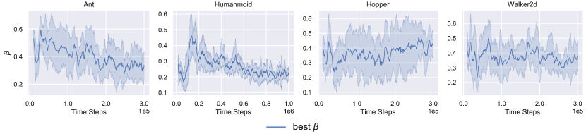
Figure 5: Visualisations of learned best $\beta$ for RAC-SAC. RAC can always auto find the best $\beta$ for different environment to balance between under- and overestimation with simple max strategy.

4.3 Variants of RAC

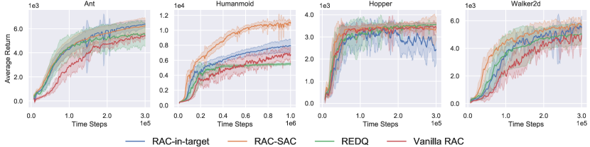
Figure 6: Performance of RAC and its variants.

To study the role of uncertainty punished Q-learning(UPQ), we implement two variants of RAC:

Vanilla RAC. Vanilla RAC uses UPQ with a constant $\beta$ to replace in-target minimization in REDQ resulting in simple vanilla RAC. The pseudocode for vanilla RAC is shown in Algorithm 3. In such a way, we can test whether UPQ improves performance compared to in-target minimization.

RAC with in-target minimization. To study the contribution of UPQ to RAC, we implement a variant of RAC-SAC which uses in-target minimization instead of UPQ to train the Q-ensemble. The pseudocode for vanilla RAC is shown in Algorithm 4.

The implement details can be found in Appendix B.3 and B.4. Results in figure 6 show that the performance of vanilla RAC is just as good as REDQ for most of the training. Compared with RAC-SAC, lower performance of vanilla RAC indicates other components of RAC-SAC are critical to performance.

In Humanmoid, the performance of RAC with in-target minimization is significantly lower than that of RAC-SAC which means UPQ is essential for RAC-SAC.

4.4 Ablation study

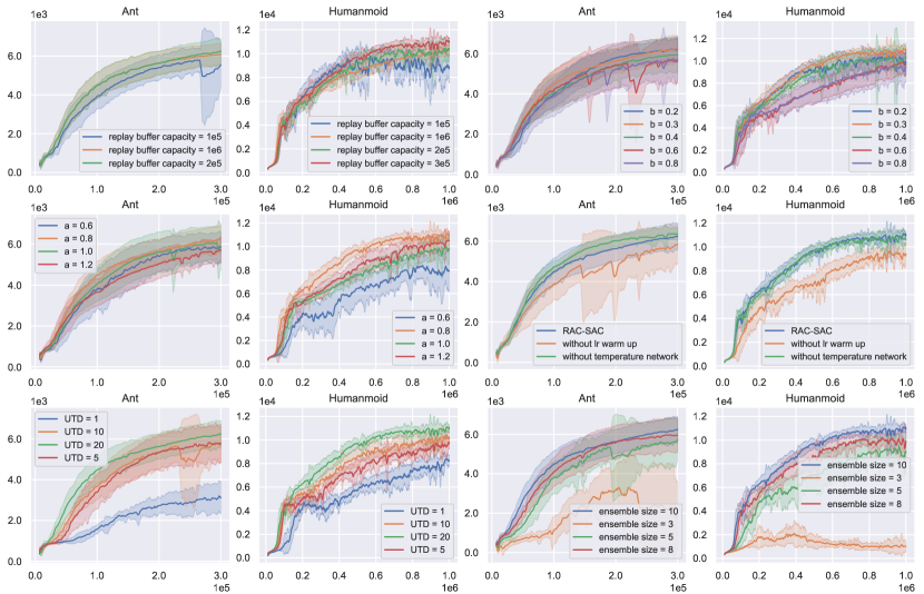
Figure 7: Results of ablations for RAC-SAC. Results are averaged over 8 seeds, ± std is shaded. The horizontal axis indicates number of time steps. The vertical axis indicates the average undiscounted return.

Smaller replay buffer capacity. In this experiment we vary the replay buffer capacity in $\{5\times 10^{4},10^{5},2\times 10^{5},3\times 10^{5},10^{6}\}$. The results in figure 7 show that RAC-SAC can benefit from a smaller capacity, but will be hurt when the capacity is excessively small.

Optimistic exploration. We vary RAC-SAC with $b\in\{0.2,0.3,0.4,0.6,0.8\}$ for exploration distribution $U_{2}[0,b]$. The results in figure 7 show that exploratory policies become more conservative with $b$ increasing, and the performance of RAC-SAC gradually declines. The increasing standard deviation means that more and more agents fall into suboptimal policies. But if $b$ is too small, the lack of exploratory diversity will cause performance degradation.

Training distribution. We vary RAC-SAC with $a\in\{0.4,0.6,0.8,1.0,1.2\}$ for training distribution $U_{1}[0,a]$. The results in figure 7 show that the average bias becomes stable with $a$ increasing. The $Q_{\theta}$ estimates will suffer a large negative bias when $a$ is too large, which make policies too conservative.

Independent temperature network. We implement a variant of RAC-SAC whose temperature is adjusted following rules (5) instead of using a temperature network. Figure 7 shows that an independent temperature network has a relatively small impact on RAC-SAC performance. Figure 11 in Appendix C shows temperatures learned by the temperature network belong to different $\beta$ at some time steps.

Update-To-Data (UTD) ratio. Figure 7 shows performance of RAC-SAC under UTD ratio values $G\in\{1,5,10,20\}$. The results suggest higher UTD values significantly improve the sample efficiency of RAC-SAC, with $G=20$ giving the best result.

Ensemble size. We vary ensemble size $N\in\{3,5,8,10\}$. The results in figure 7 suggest a larger ensemble size can stabilize average bias and decrease std of bias bringing about better performance.

Learning rate warm up. RAC-SAC applies a linear learning rate warm-up strategy (see details in Appendix B) to stable early learning. The results in figure 7 demonstrate that the early learning of RAC-SAC will be unstable without the learning rate warm-up.

5 Conclusion

In this paper, we present RAC to balance value under- and overestimation by involving policies with different value confidence-bonds. RAC is a simple ensemble method, which can be used to improve off-policy reinforcement learning algorithms. Experiments show advantageous properties of RAC: low value approximation error and brilliant sample efficiency. Results on continuous control benchmarks suggest that RAC consistently improves performances of existing off-policy RL algorithms, such as SAC and TD3.

Our results suggest that directly incorporate uncertainty to value functions and learning a powerful policy family can provide a promising avenue for improved sample efficiency and performance, and further exploration of ensemble methods, including high-level policies or more rich policy classes is an exciting avenue for future work.

Appendix:

Balancing Value Underestimation and Overestimation with Realistic Actor-Critic

Appendix A Experiments Setups and methodology

A.1 Reproducing the Baselines

The baseline algorithms are REDQ [10], MBPO [20], SAC [17], TD3 [15] and TQC [27]. All hyper-parameters we used for evaluation are the same as those in the original papers. For MBPO, REDQ, TD3 and TQC, we use the authors’s code. For SAC, we implement it following Haarnoja et al. [17], and results we obtained are similar to previously reported results.

A.2 Evaluation method

For all training instances, the policies are evaluated every $R_{eval}=10^{3}$ time steps. At each evaluation phase, the agent fixes its policy, deterministically interacts with the same environment separate to obtain $10$ episodic rewards. The mean and standard deviation of these $10$ episodic rewards is the performance metrics of the agent at the evaluation phase.

In the case of RAC, we employ a discrete number $H$ of values $\left\{\beta_{i}\right\}_{i=1}^{H}$ to get $H$ policies:

$$\beta_{i}=b/H\cdot i,i=1,\ldots,H.$$ (20)

Each of the $H$ policies fixes its policy as the one at the evaluation phase and deterministically interacts with the environment with the fixed policy to obtain $10$ episodic rewards. The $10$ episodic rewards are averaged for each policy, and then the maximum of the $10$-episode-average rewards of the $H$ policies is taken as the performance at that evaluation phase.

We performed this operation for $8$ different random seeds used in the computational packages(numpy, pytorch) and environments(openai gym), and the mean and standard deviation of the learning curve are obtained from these $8$ simulations.

For all experiments, our learning curves show the total undiscounted return.

A.3 The normalized values bias estimation

Given a state-action pair, the normalized values bias is defined as:

$$\left(\bar{Q}_{\theta}(\mathbf{s},\mathbf{a})-Q^{\pi}(\mathbf{s},\mathbf{a})\right)/\left|E_{\bar{\mathbf{s}},\bar{\mathbf{a}}\sim\pi}\left[Q^{\pi}(\bar{\mathbf{s}},\bar{\mathbf{a}})\right]\right|,$$ (21)

where

• $Q^{\pi}(\mathbf{s},\mathbf{a})$ be the action-value function for policy $\pi$ using the standard infinite-horizon discounted Monte Carlo return definition.

• $\bar{Q}_{\theta}(\mathbf{s},\mathbf{a})$ the estimated Q-value, defined as the mean of $Q_{\theta_{i}}(\mathbf{s},\mathbf{a}),i=1,\ldots,N$.

For RAC, the normalized values bias is defined as:

$$\left(\bar{Q}_{\theta}(\mathbf{s},\mathbf{a},\beta^{*})-Q^{\pi^{*}}(\mathbf{s},\mathbf{a})\right)/\left|E_{\bar{s},\bar{a}\sim\pi^{*}}\left[Q^{\pi^{*}}(\bar{\mathbf{s}},\bar{\mathbf{a}})\right]\right|,$$ (22)

where

• $\pi^{*}$ is the best-performing policy in the evaluation among $H$ policies A.2.

• $Q^{\pi^{*}}(\mathbf{s},\mathbf{a})$ be the action-value function for policy $\pi^{*}$ using the standard infinite-horizon discounted Monte Carlo return definition.

• $\bar{Q}_{\theta}(\mathbf{s},\mathbf{a},\beta^{*})$ the estimated Q-value using $Q_{\theta}$ of $\beta^{*}$ which corresponds to the policy $\pi^{*}$, defined as the mean of $Q_{\theta_{i}}(\mathbf{s},\mathbf{a},\beta^{*}),i=1,\ldots,N$.

To get various target state-action pairs, we first execute the policy in the environment to obtain 100 state-action pairs and then sample the target state-action pair from them without repetition. Starting from the target state-action pair, running the Monte Carlo processes until the max step limit is reached. Table 3 lists common parameters of the normalized values bias estimation.

Table 3: Parameters of the normalized values bias estimation

Parameter		Value
	number of Monte Carlo process	20
	number of target state-action pairs	20
	Max step limit	1500

Appendix B Hyperparameters and implementation details

We implement all RAC algorithms with Pytorch [35] and use Ray[tune] [30] to build and run distributed applications. For all the algorithms and variants, we first obtain $5000$ data points by randomly sampling actions from the action space without making any parameter updates. In order to stabilize early learning of critics, a linear learning rate warm up strategy is applied to critics in the start stage of training for RAC and its variants:

$$l=l_{init}(1-p)+p\cdot l_{target},p=\operatorname{clip}(\frac{t-t_{start}}{t_{target}-t_{start}},0,1),$$ (23)

where $l$ is current learning rate, $l_{init}$ is the initial value of learning rate, $l_{target}$ is the target value of learning rate, $t_{start}$ is the time steps to start adjusting the learning rate, $t_{target}$ is the time steps to arrive at $l_{target}$.

For all RAC algorithms and variants, We parameterize both the actor and critics with feed-forward neural networks with $256$ and $256$ hidden nodes respectively, with rectified linear units (ReLU) [32] between each layer. $\beta$ is log-scaled before input into actors and critics. In order to prevent $\beta$ sample from being zero, a small value $\varepsilon=10^{-7}$ is added to the left side of $U_{1}$ and $U_{2}$ to be $U_{1}[\varepsilon,a]$ and $U_{2}[\varepsilon,b]$. Weights of all networks are initialized with Kaiming Uniform Initialization [19], and biases are zero-initialized. For all environments, we normalize actions to a range of $[-1,1]$.

B.1 RAC-SAC algorithm

Here, the policy is modeled as a Gaussian with mean and covariance given by neural networks to handle continuous action spaces. The way RAC optimize the policy makes use of the reparameterization trick [25, 17], in which a sample from is drawn by computing a deterministic function of the state, policy parameters, and independent noise:

$$\tilde{\mathbf{a}}_{\phi}(\mathbf{s},\beta,\xi)=\tanh\left(\mu_{\phi}(\mathbf{s},\beta)+\sigma_{\phi}(\mathbf{s},\beta)\odot\xi\right),\quad\xi\sim\mathcal{N}(0,I).$$ (24)

The actor network outputs the Gaussian’s means and log-scaled covariance, and the log-scaled covariance is clipped in a range of $[-10,2]$ to avoid extreme values. The actions are bounded to a finite interval by applying an invertible squashing function ($tanh$) to the Gaussian samples, and the log-likelihood of actions is calculated by the Squashed Gaussian Trick [17].

The temperature is parameterized by a one layer feedforward neural network $T_{\psi}$ of $64$ with rectified linear units (ReLU). To prevent temperature be negative, we parameterize temperature as:

$$\alpha_{\psi}(\beta)=e^{T_{\psi}(\operatorname{log}(\beta))+\xi},$$ (25)

where $\xi$ is constant controlling the initial temperature, $\operatorname{log}(\beta)$ is log-scaled $\beta$, $T_{\psi}(\operatorname{log}(\beta))$ is the output of the neural network.

B.2 RAC-TD3 algorithm

We implement RAC-TD3 referring to https://github.com/sfujim/TD3. A final $tanh$ unit following the output of the actor. Different from TD3, we did not use a target network for actor and delayed policy updates. For each update of critics, a small amount of random noise is added to the policy and averaging over mini-batches:

$$y=r+\gamma\left[\bar{Q}_{\bar{\theta}}(\mathbf{s^{\prime}},\mathbf{a^{\prime}},\beta)-\beta\hat{s}({Q}_{\bar{\theta}}(\mathbf{s^{\prime}},\mathbf{a^{\prime}},\beta))\right],$$ (26)

$$\mathbf{a^{\prime}}=\operatorname{clip}(\pi_{\phi}\left(\cdot\mid\mathbf{s^{\prime}},\beta\right)+\epsilon,-1,1),$$ (27)

$$\epsilon\sim\operatorname{clip}(\mathcal{N}(0,\sigma),-c,c).$$ (28)

The extended policy $\pi_{\phi}$ is updated by minimizing the following object:

$$\mathcal{L}^{\tt RAC-TD3}_{\tt actor}(\phi)=\mathbb{E}_{\mathbf{s}\sim\mathcal{B},\beta\sim U_{1}}\left[-\bar{Q}_{\theta}\left(\mathbf{a},\mathbf{s},\beta\right)\right],\mathbf{a}=\pi_{\phi}\left(\cdot\mid\mathbf{s},\beta\right).$$ (29)

The pseudocode for RAC-TD3 is shown in Algorithm 2.

Algorithm 2 RAC: TD3 version

1:Initialize actor network $\phi$, $N$ critic networks $\theta_{i},i=1,\ldots,N$, empty replay buffer $\mathcal{B}$, target network $\bar{\theta_{i}}\longleftarrow\theta_{i}$, for $i=1,2,\ldots,N$, uniform distribution $\mathcal{U}_{1}$ and $U_{2}$

2:for each iteration do

3:     execute an action $\mathbf{a}=\pi_{\phi}\left(\cdot\mid\mathbf{s},\beta\right)+\epsilon,\epsilon\sim\mathcal{N}(0,\sigma),\beta\sim U_{2}$. Observe reward $r$, new state $\mathbf{s^{\prime}}$

4:     Store transition tuple $\mathcal{B}\leftarrow\mathcal{B}\cup\left\{\left(\mathbf{s},\mathbf{a},r,\mathbf{s^{\prime}}\right)\right\}$

5:     for $G$ updates do

6:         Sample random minibatch $\{\tau_{j}\}_{j=1}^{B}\sim\mathcal{B}$, $\{\beta_{m}\}_{m=1}^{B}\sim U_{1}$

7:         Compute the Q target (26)

8:         for $i=1,...,N$ do

9:              Update $\theta_{i}$ by minimize $\mathcal{L}^{\tt RAC}_{\tt critic}$ (17)

10:              Update target networks with $\bar{\theta_{i}}\leftarrow\rho\bar{\theta_{i}}+(1-\rho)\theta_{i}$

11:         end for

12:     end for

13:     Update actor parameters $\phi$ by minimize $\mathcal{L}^{\tt RAC-TD3}_{\tt actor}$ (29)

14:end for

B.3 Vanilla RAC algorithm

For vanilla RAC, UVFA is not needed as $\beta$ is a constant. The actor is updated by minimizing the following object:

$$\mathcal{L}^{\tt{vanillaRAC}}_{\tt actor}(\phi)=\mathbb{E}_{\mathbf{s}\sim\mathcal{B},\mathbf{a}\sim\pi_{\phi}}\left[\alpha\log\left(\pi_{\phi}\left(\mathbf{a}\mid\mathbf{s}\right)\right)-\bar{Q}_{\theta}\left(\mathbf{a},\mathbf{s}\right)\right].$$ (30)

The pseudocode for Vanilla RAC is shown in Algorithm 3. Figture 8, 9, and 10 shows performance and Q bias of Vanilla RAC with different $\beta$.

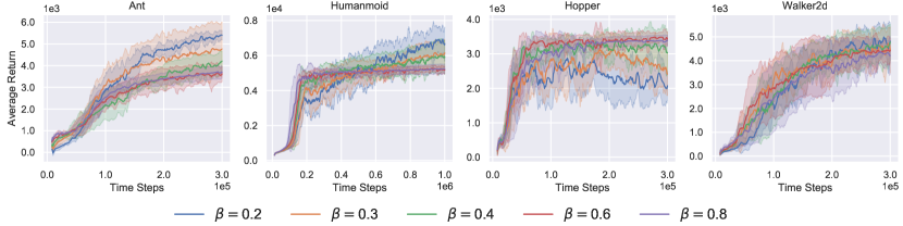
Figure 8: Performance of Vanilla RAC with different $\beta$.

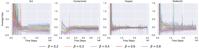
Figure 9: Mean of normalized Q bias for Vanilla RAC with different $\beta$.

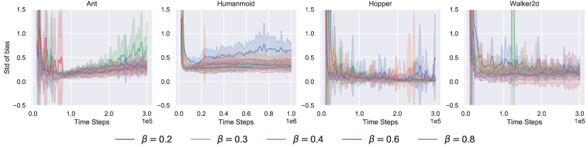
Figure 10: Std of normalized Q bias for Vanilla RAC with different $\beta$.

Algorithm 3 Vanilla RAC

1:Initialize actor network $\phi$, $N$ critic networks $\theta_{i},i=1,\ldots,N$, empty replay buffer $\mathcal{B}$, target network $\bar{\theta_{i}}\longleftarrow\theta_{i}$, for $i=1,2,\ldots,N$

2:for each iteration do

3:     execute an action $\mathbf{a}\sim\pi_{\phi}\left(\cdot\mid s\right)$. Observe reward $r$, new state $\mathbf{s^{\prime}}$

4:     Store transition tuple $\mathcal{B}\leftarrow\mathcal{B}\cup\left\{\left(\mathbf{s},\mathbf{a},r,\mathbf{s^{\prime}}\right)\right\}$

5:     for $G$ updates do

6:         Sample random minibatch $\{\tau_{j}\}_{j=1}^{B}\sim\mathcal{B}$

7:         Compute the Q target (6)

8:         for $i=1,\ldots,N$ do

9:              Update $\theta_{i}$ by minimize $\mathcal{L}_{\tt critic}$ (2)

10:              Update target networks with $\bar{\theta_{i}}\leftarrow\rho\bar{\theta_{i}}+(1-\rho)\theta_{i}$

11:         end for

12:     end for

13:     Update actor parameters $\phi$ by minimize $\mathcal{L}^{\tt vanillaRAC}_{\tt actor}$ (30)

14:     Update temperature $\alpha$ by minimize $\mathcal{L}_{\tt temp}$ (5)

15:end for

B.4 RAC with in-target minimization

We implement RAC with in-target minimization referring to authors’s code https://github.com/watchernyu/REDQ. The critics and actor are extended as $Q_{\theta_{i}}(\mathbf{s},\mathbf{a},k)$ and $\pi_{\phi}\left(\cdot\mid\mathbf{s^{\prime}},k\right)$, $U_{1}$ is a uniform traning distribution $\mathcal{U}[1,a]$, $a>1$, $k\sim U_{1}$ that determine the size of the random subset $\mathcal{M}$. When $k$ is not an integer, the size of $\mathcal{M}$ will be sample beweetn $\operatorname{floor}(k)$ and $\operatorname{floor}(k+1)$ according to the Bernoulli distribution $\mathcal{B}(p)$ with parameter $p=k-\operatorname{floor}(k)$, where $\operatorname{floor}$ is a round-towards-zero operator.

An independent temperature network $\alpha_{\psi}$ parameterized by $\psi$ is updated with the following object:

$$\mathcal{L}^{\tt RAC}_{\tt temp}(\psi)=\mathbb{E}_{\mathbf{s}\sim\mathcal{B},\mathbf{a}\sim\pi_{\phi},k\sim U_{1}}\left[-\alpha_{\psi}(k)\log\pi_{\phi}\left(\mathbf{a}\mid\mathbf{s},k\right)-\alpha_{\psi}(k)\overline{\mathcal{H}}\right].$$ (31)

In-target minimization is used to calculate the target $y$:

$$y=r+\gamma\mathbb{E}_{\mathbf{a^{\prime}}\sim\pi_{\phi}}\left[\min_{i\in\mathcal{M}}Q_{\bar{\theta_{i}}}\left(\mathbf{s^{\prime}},\mathbf{a^{\prime}},k\right)-\alpha_{\psi}(k)\log\pi_{\phi}\left(\mathbf{a^{\prime}}\mid\mathbf{s^{\prime}},k\right)\right],$$ (32)

Then each $Q_{\theta_{i}}(\mathbf{s},\mathbf{a},k)$ is updated with the same target:

$$\mathcal{L}^{\tt RAC}_{\tt critic}(\theta_{i})=\mathbb{E}_{\tau_{t}\sim\mathcal{B},k\sim U_{1}}[\left(Q_{\theta_{i}}(\mathbf{s},\mathbf{a},k)-y\right)^{2}].$$ (33)

The extended policy $\pi_{\phi}$ is updated by minimizing the following object:

$$\mathcal{L}^{\tt RAC}_{\tt actor}(\phi)=\mathbb{E}_{\mathbf{s}\sim\mathcal{B},k\sim U_{1}}\left[\mathbb{E}_{\mathbf{a}\sim\pi_{\phi}}\left[\alpha_{\psi}(k)\log\left(\pi_{\phi}\left(\mathbf{a}\mid\mathbf{s},k\right)\right)-\bar{Q}_{\theta}\left(\mathbf{a},\mathbf{s},k\right)\right]\right].$$ (34)

When interacting with the environment, obtaining exploration behavior by sample $k$ from exploration distribution $U_{2}=\mathcal{U}[1,b]$, $a>b>1$.

The pseudocode for RAC with in-target minimization is shown in Algorithm 4.

Algorithm 4 RAC with in-target minimization

1:Initialize actor network $\phi$, $N$ critic networks $\theta_{i},i=1,\ldots,N$, temperature network $\psi$, empty replay buffer $\mathcal{B}$, target network $\bar{\theta_{i}}\longleftarrow\theta_{i}$, for $i=1,2,\ldots,N$, uniform distribution $U_{1}$ and $U_{2}$

2:for each iteration do

3:     execute an action $\mathbf{a}\sim\pi_{\phi}\left(\cdot\mid\mathbf{s},k\right),k\sim U_{2}$. Observe reward $r$, new state $\mathbf{s^{\prime}}$

4:     Store transition tuple $\mathcal{B}\leftarrow\mathcal{B}\cup\left\{\left(\mathbf{s},\mathbf{a},r,\mathbf{s^{\prime}}\right)\right\}$

5:     for $G$ updates do

6:         Sample random minibatch $\{\tau_{j}\}_{j=1}^{B}\sim\mathcal{B}$, $\{k_{j}\}_{j=1}\sim U_{1}$

7:         Sample a set $\mathcal{M}$ of $k$ distinct indices from $\{1,2,\ldots,N\}$

8:         Compute the Q target (32)

9:         for $i=1,\ldots,N$ do

10:              Update $\theta_{i}$ by minimize $\mathcal{L}^{\tt RAC}_{\tt critic}$ (33)

11:              Update target networks with $\bar{\theta_{i}}\leftarrow\rho\bar{\theta_{i}}+(1-\rho)\theta_{i}$

12:         end for

13:     end for

14:     Update actor parameters $\phi$ by minimize $\mathcal{L}^{\tt RAC-SAC}_{\tt actor}$ (34)

15:     Update temperature parameters $\psi$ by minimize $\mathcal{L}^{\tt RAC}_{\tt temp}$ (31)

16:end for

B.5 Selection of hyperparameters

In order to select the hyperparameters used for RAC for all mojoco environments, which are shown in table 6, we ran a grid search with the ranges shown on table 4, and the combination with the highest cumulative rewards amount environments are selected.

Table 4: Range of hyperparameters sweeps

Hyperparameters		Value
Shared
	Update-To-Data (UTD) ratio ($G$)	{1, 5, 10, 20}
	ensemble size ($N$)	{2, 5, 10}
RAC-SAC
	initial temperature coefficient ($\xi$)	{$-5,-2,0$}
	right side of exploitation distribution $U_{1}$ ($a$)	{$0.6,0.8,1.0,1.2$}
	right side of exploration distribution $U_{2}$ ($b$)	{$0.2,0.3,0.4,0.6,0.8$}
	replay buffer capacity	{$0.5\times 10^{5},10^{5},2\times 10^{5},3\times 10^{5},10^{6}$}
RAC-TD3
	right side of exploitation distribution $U_{1}$ ($a$)	{$0.6,0.8,1.0,1.2$}
	right side of exploration distribution $U_{2}$ ($b$)	{$0.2,0.3,0.4,0.6,0.8$}
	replay buffer capacity	{$0.5\times 10^{5},10^{5},2\times 10^{5},3\times 10^{5},10^{6}$}
Vanilla RAC
	uncertainty punishment ($\beta$)	{$0.2,0.3,0.4,0.6,0.8$}
RAC with in-target minimization
	right side of exploitation distribution $U_{1}$ ($a$)	{$2,2.5,3,4$}
	right side of exploration distribution $U_{2}$ ($b$)	{$1.25,1.5,1.75,2$}

B.6 Hyperparameter setting

Table 5 and 6 lists the hyperparameters for RAC and variants used in experiments.

Table 5: Shared hyperparameters

Hyperparameters		Value
	optimizer	Adam [24]
	actor learning rate	$3\times 10^{-4}$
	temperature learning rate	$3\times 10^{-4}$
	initial critic learning rate ($l_{init}$)	$3\times 10^{-5}$
	target critic learning rate ($l_{target}$)	$3\times 10^{-4}$
	time steps to start learning rate adjusting ($t_{start}$)	5000
	time steps to reach target learning rate ($t_{target}$)	$10^{4}$
	number of hidden layers (for $\phi$ and $\theta_{i}$)	2
	number of hidden units per layer (for $\phi$ and $\theta_{i}$)	256
	number of hidden layers (for $T_{\psi}$)	1
	number of hidden units per layer (for $T_{\psi}$)	64
	discount ($\gamma$)	0.99
	nonlinearity	ReLU
	evaluation frequence	$10^{3}$
	minibatch size	256
	target smoothing coefficient ($\rho$)	0.005
	Update-To-Data (UTD) ratio ($G$)	20
	ensemble size ($N$)	10
	number of evaluation episodes	10
	initial random time steps	5000
	frequence of delayed policy updates	1
	log-scaled covariance clip range	$[-10,2]$
	number of discrete policies for evaluation ($H$)	12

Table 6: Specific Hyperparameters

Hyperparameters		Value
RAC-SAC
	initial temperature coefficient ($\xi$)	$-5$
	exploitation distribution $U_{1}$	$\mathcal{U}[10^{-7},0.8]$
	exploration distribution $U_{2}$	$\mathcal{U}[10^{-7},0.3]$
RAC-TD3
	exploration noisy	$\mathcal{N}(0,0.1)$
	policy noisy ($\sigma$)	$0.2$
	policy noisy clip ($c$)	$0.5$
	traning distribution $U_{1}$	$\mathcal{U}[10^{-7},0.8]$
	exploration distribution $U_{2}$	$\mathcal{U}[10^{-7},0.3]$
Vanilla RAC
	initial temperature	$\exp(-3)$
	uncertainty punishment ($\beta$)	0.3
RAC with in-target minimization
	initial temperature coefficient ($\xi$)	$-5$
	exploitation distribution $U_{1}$	$\mathcal{U}[1,1.5]$
	exploration distribution $U_{2}$	$\mathcal{U}[1,2.0]$

Table 7: Environment dependent hyperparameters

Hyperparameters		Humanmoid	Walker	Ant	Hopper
RAC-SAC
	replay buffer capacity	$3\times 10^{5}$	$10^{5}$	$2\times 10^{5}$	$1\times 10^{6}$
RAC-TD3
	replay buffer capacity	$3\times 10^{5}$	$10^{5}$	$2\times 10^{5}$	$1\times 10^{6}$
Vanilla RAC
	replay buffer capacity	$10^{6}$	$10^{6}$	$10^{6}$	$10^{6}$
	uncertainty punishment ($\beta$)	0.2	0.3	0.2	0.2
RAC with in-target minimization
	replay buffer capacity	$3\times 10^{5}$	$10^{5}$	$2\times 10^{5}$	$1\times 10^{6}$

Appendix C Visualisations of learned temperatures

The figure 11 shows the visualization of learned temperatures with respect to different $\beta$ during training. The figure demonstrates that learned temperatures are quite different, it is difficult to take into account the temperature of different $\beta$ with a single temperature.

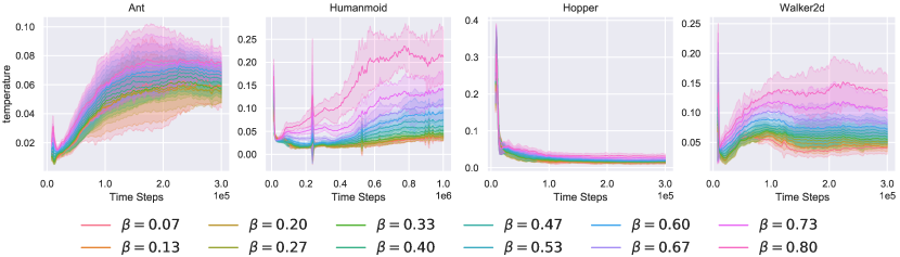
Figure 11: Visualisations of learned temperatures for RAC-SAC with different $\beta$.

References

- Abdar et al. [2021] Abdar, Moloud, Pourpanah, Farhad, Hussain, Sadiq, Rezazadegan, Dana, Liu, Li, Ghavamzadeh, Mohammad, Fieguth, Paul, Cao, Xiaochun, Khosravi, Abbas, Acharya, U Rajendra, et al. A review of uncertainty quantification in deep learning: Techniques, applications and challenges. Information Fusion, 2021.
- Amos et al. [2018] Amos, Brandon, Dinh, Laurent, Cabi, Serkan, Rothörl, Thomas, Colmenarejo, Sergio Gómez, Muldal, Alistair, Erez, Tom, Tassa, Yuval, de Freitas, Nando, and Denil, Misha. Learning awareness models. arXiv preprint arXiv:1804.06318, 2018.
- Anschel et al. [2017] Anschel, Oron, Baram, Nir, and Shimkin, Nahum. Averaged-dqn: Variance reduction and stabilization for deep reinforcement learning. In International Conference on Machine Learning, pp. 176–185. PMLR, 2017.
- Badia et al. [2020a] Badia, Adrià Puigdomènech, Piot, Bilal, Kapturowski, Steven, Sprechmann, Pablo, Vitvitskyi, Alex, Guo, Zhaohan Daniel, and Blundell, Charles. Agent57: Outperforming the atari human benchmark. In International Conference on Machine Learning, pp. 507–517. PMLR, 2020a.
- Badia et al. [2020b] Badia, Adrià Puigdomènech, Sprechmann, Pablo, Vitvitskyi, Alex, Guo, Daniel, Piot, Bilal, Kapturowski, Steven, Tieleman, Olivier, Arjovsky, Martín, Pritzel, Alexander, Bolt, Andew, et al. Never give up: Learning directed exploration strategies. arXiv preprint arXiv:2002.06038, 2020b.
- Brafman & Tennenholtz [2002] Brafman, Ronen I and Tennenholtz, Moshe. R-max-a general polynomial time algorithm for near-optimal reinforcement learning. Journal of Machine Learning Research, 3(Oct):213–231, 2002.
- Brockman et al. [2016] Brockman, Greg, Cheung, Vicki, Pettersson, Ludwig, Schneider, Jonas, Schulman, John, Tang, Jie, and Zaremba, Wojciech. Openai gym. arXiv preprint arXiv:1606.01540, 2016.
- Chen & Peng [2019] Chen, Gang and Peng, Yiming. Off-policy actor-critic in an ensemble: Achieving maximum general entropy and effective environment exploration in deep reinforcement learning. arXiv preprint arXiv:1902.05551, 2019.
- Chen et al. [2017] Chen, Richard Y, Sidor, Szymon, Abbeel, Pieter, and Schulman, John. Ucb exploration via q-ensembles. arXiv preprint arXiv:1706.01502, 2017.
- Chen et al. [2021] Chen, Xinyue, Wang, Che, Zhou, Zijian, and Ross, Keith. Randomized ensembled double q-learning: Learning fast without a model. arXiv preprint arXiv:2101.05982, 2021.
- Ciosek et al. [2019] Ciosek, Kamil, Vuong, Quan, Loftin, Robert, and Hofmann, Katja. Better exploration with optimistic actor-critic. arXiv preprint arXiv:1910.12807, 2019.
- Dorner [2021] Dorner, Florian E. Measuring progress in deep reinforcement learning sample efficiency. arXiv preprint arXiv:2102.04881, 2021.
- Dulac-Arnold et al. [2020] Dulac-Arnold, Gabriel, Levine, Nir, Mankowitz, Daniel J, Li, Jerry, Paduraru, Cosmin, Gowal, Sven, and Hester, Todd. An empirical investigation of the challenges of real-world reinforcement learning. arXiv preprint arXiv:2003.11881, 2020.
- Dusenberry et al. [2020] Dusenberry, Michael, Jerfel, Ghassen, Wen, Yeming, Ma, Yian, Snoek, Jasper, Heller, Katherine, Lakshminarayanan, Balaji, and Tran, Dustin. Efficient and scalable bayesian neural nets with rank-1 factors. In International conference on machine learning, pp. 2782–2792. PMLR, 2020.
- Fujimoto et al. [2018] Fujimoto, Scott, Hoof, Herke, and Meger, David. Addressing function approximation error in actor-critic methods. In International Conference on Machine Learning, pp. 1587–1596. PMLR, 2018.
- Goyal et al. [2019] Goyal, Anirudh, Sodhani, Shagun, Binas, Jonathan, Peng, Xue Bin, Levine, Sergey, and Bengio, Yoshua. Reinforcement learning with competitive ensembles of information-constrained primitives. arXiv preprint arXiv:1906.10667, 2019.
- Haarnoja et al. [2018] Haarnoja, Tuomas, Zhou, Aurick, Hartikainen, Kristian, Tucker, George, Ha, Sehoon, Tan, Jie, Kumar, Vikash, Zhu, Henry, Gupta, Abhishek, Abbeel, Pieter, et al. Soft actor-critic algorithms and applications. arXiv preprint arXiv:1812.05905, 2018.
- Havasi et al. [2020] Havasi, Marton, Jenatton, Rodolphe, Fort, Stanislav, Liu, Jeremiah Zhe, Snoek, Jasper, Lakshminarayanan, Balaji, Dai, Andrew M, and Tran, Dustin. Training independent subnetworks for robust prediction. arXiv preprint arXiv:2010.06610, 2020.
- He et al. [2015] He, Kaiming, Zhang, Xiangyu, Ren, Shaoqing, and Sun, Jian. Delving deep into rectifiers: Surpassing human-level performance on imagenet classification. In Proceedings of the IEEE international conference on computer vision, pp. 1026–1034, 2015.
- Janner et al. [2019] Janner, Michael, Fu, Justin, Zhang, Marvin, and Levine, Sergey. When to trust your model: Model-based policy optimization. arXiv preprint arXiv:1906.08253, 2019.
- Jung et al. [2020] Jung, Whiyoung, Park, Giseung, and Sung, Youngchul. Population-guided parallel policy search for reinforcement learning. arXiv preprint arXiv:2001.02907, 2020.
- Kalweit & Boedecker [2017] Kalweit, Gabriel and Boedecker, Joschka. Uncertainty-driven imagination for continuous deep reinforcement learning. In Conference on Robot Learning, pp. 195–206. PMLR, 2017.
- Kim et al. [2018] Kim, Hyoungseok, Kim, Jaekyeom, Jeong, Yeonwoo, Levine, Sergey, and Song, Hyun Oh. Emi: Exploration with mutual information. arXiv preprint arXiv:1810.01176, 2018.
- Kingma & Ba [2014] Kingma, Diederik P and Ba, Jimmy. Adam: A method for stochastic optimization. arXiv preprint arXiv:1412.6980, 2014.
- Kingma & Welling [2013] Kingma, Diederik P and Welling, Max. Auto-encoding variational bayes. arXiv preprint arXiv:1312.6114, 2013.
- Kumar et al. [2020] Kumar, Aviral, Gupta, Abhishek, and Levine, Sergey. Discor: Corrective feedback in reinforcement learning via distribution correction. arXiv preprint arXiv:2003.07305, 2020.
- Kuznetsov et al. [2020] Kuznetsov, Arsenii, Shvechikov, Pavel, Grishin, Alexander, and Vetrov, Dmitry. Controlling overestimation bias with truncated mixture of continuous distributional quantile critics. In International Conference on Machine Learning, pp. 5556–5566. PMLR, 2020.
- Lan et al. [2020] Lan, Qingfeng, Pan, Yangchen, Fyshe, Alona, and White, Martha. Maxmin q-learning: Controlling the estimation bias of q-learning. arXiv preprint arXiv:2002.06487, 2020.
- Lee et al. [2020] Lee, Kimin, Laskin, Michael, Srinivas, Aravind, and Abbeel, Pieter. Sunrise: A simple unified framework for ensemble learning in deep reinforcement learning. arXiv preprint arXiv:2007.04938, 2020.
- Liaw et al. [2018] Liaw, Richard, Liang, Eric, Nishihara, Robert, Moritz, Philipp, Gonzalez, Joseph E, and Stoica, Ion. Tune: A research platform for distributed model selection and training. arXiv preprint arXiv:1807.05118, 2018.
- Lyle et al. [2021] Lyle, Clare, Rowland, Mark, Ostrovski, Georg, and Dabney, Will. On the effect of auxiliary tasks on representation dynamics. In International Conference on Artificial Intelligence and Statistics, pp. 1–9. PMLR, 2021.
- Nair & Hinton [2010] Nair, Vinod and Hinton, Geoffrey E. Rectified linear units improve restricted boltzmann machines. In Icml, 2010.
- Osband et al. [2016] Osband, Ian, Blundell, Charles, Pritzel, Alexander, and Van Roy, Benjamin. Deep exploration via bootstrapped dqn. arXiv preprint arXiv:1602.04621, 2016.
- Parker-Holder et al. [2020] Parker-Holder, Jack, Pacchiano, Aldo, Choromanski, Krzysztof, and Roberts, Stephen. Effective diversity in population-based reinforcement learning. arXiv preprint arXiv:2002.00632, 2020.
- Paszke et al. [2019] Paszke, Adam, Gross, Sam, Massa, Francisco, Lerer, Adam, Bradbury, James, Chanan, Gregory, Killeen, Trevor, Lin, Zeming, Gimelshein, Natalia, Antiga, Luca, et al. Pytorch: An imperative style, high-performance deep learning library. arXiv preprint arXiv:1912.01703, 2019.
- Pathak et al. [2019] Pathak, Deepak, Gandhi, Dhiraj, and Gupta, Abhinav. Self-supervised exploration via disagreement. In International Conference on Machine Learning, pp. 5062–5071. PMLR, 2019.
- Peer et al. [2021] Peer, Oren, Tessler, Chen, Merlis, Nadav, and Meir, Ron. Ensemble bootstrapping for q-learning. arXiv preprint arXiv:2103.00445, 2021.
- Pendrith et al. [1997] Pendrith, Mark D, Ryan, Malcolm RK, et al. Estimator variance in reinforcement learning: Theoretical problems and practical solutions. University of New South Wales, School of Computer Science and Engineering, 1997.
- Rashid et al. [2020] Rashid, Tabish, Peng, Bei, Boehmer, Wendelin, and Whiteson, Shimon. Optimistic exploration even with a pessimistic initialisation. arXiv preprint arXiv:2002.12174, 2020.
- Saphal et al. [2020] Saphal, Rohan, Ravindran, Balaraman, Mudigere, Dheevatsa, Avancha, Sasikanth, and Kaul, Bharat. Seerl: Sample efficient ensemble reinforcement learning. arXiv preprint arXiv:2001.05209, 2020.
- Schaul et al. [2015] Schaul, Tom, Horgan, Daniel, Gregor, Karol, and Silver, David. Universal value function approximators. In International conference on machine learning, pp. 1312–1320. PMLR, 2015.
- Srivastava et al. [2014] Srivastava, Nitish, Hinton, Geoffrey, Krizhevsky, Alex, Sutskever, Ilya, and Salakhutdinov, Ruslan. Dropout: a simple way to prevent neural networks from overfitting. The journal of machine learning research, 15(1):1929–1958, 2014.
- Sutton & Barto [2018] Sutton, Richard S and Barto, Andrew G. Reinforcement learning: An introduction. MIT press, 2018.
- Thrun & Schwartz [1993] Thrun, Sebastian and Schwartz, Anton. Issues in using function approximation for reinforcement learning. In Proceedings of the Fourth Connectionist Models Summer School, pp. 255–263. Hillsdale, NJ, 1993.
- Todorov et al. [2012] Todorov, Emanuel, Erez, Tom, and Tassa, Yuval. Mujoco: A physics engine for model-based control. In 2012 IEEE/RSJ International Conference on Intelligent Robots and Systems, pp. 5026–5033. IEEE, 2012.
- Warwick & Lininger [1975] Warwick, Donald P and Lininger, Charles A. The sample survey: Theory and practice. McGraw-Hill, 1975.
- Wen et al. [2020] Wen, Yeming, Tran, Dustin, and Ba, Jimmy. Batchensemble: an alternative approach to efficient ensemble and lifelong learning. arXiv preprint arXiv:2002.06715, 2020.
- Wenzel et al. [2020] Wenzel, Florian, Snoek, Jasper, Tran, Dustin, and Jenatton, Rodolphe. Hyperparameter ensembles for robustness and uncertainty quantification. arXiv preprint arXiv:2006.13570, 2020.
- Wu et al. [2021] Wu, Yue, Zhai, Shuangfei, Srivastava, Nitish, Susskind, Joshua, Zhang, Jian, Salakhutdinov, Ruslan, and Goh, Hanlin. Uncertainty weighted actor-critic for offline reinforcement learning. arXiv preprint arXiv:2105.08140, 2021.
- Zheng12 et al. [2018] Zheng12, Zhuobin, Yuan, Chun, Lin12, Zhihui, and Cheng12, Yangyang. Self-adaptive double bootstrapped ddpg. International Joint Conference on Artificial Intelligence, 2018.
- Ziebart [2010] Ziebart, Brian D. Modeling purposeful adaptive behavior with the principle of maximum causal entropy. Carnegie Mellon University, 2010.