Coordinated Beamforming in Quantized Massive MIMO Systems with Per-Antenna Constraints

Abstract

In this work, we present a solution for coordinated beamforming for large-scale downlink (DL) communication systems with low-resolution data converters when employing a per-antenna power constraint that limits the maximum antenna power to alleviate hardware cost. To this end, we formulate and solve the antenna power minimax problem for the coarsely quantized DL system with target signal-to-interference-plus-noise ratio requirements. We show that the associated Lagrangian dual with uncertain noise covariance matrices achieves zero duality gap and that the dual solution can be used to obtain the primal DL solution. Using strong duality, we propose an iterative algorithm to determine the optimal dual solution, which is used to compute the optimal DL beamformer. We further update the noise covariance matrices using the optimal DL solution with an associated subgradient and perform projection onto the feasible domain. Through simulation, we evaluate the proposed method in maximum antenna power consumption and peak-to-average power ratio which are directly related to hardware efficiency.

I Introduction

Massive multiple-input-multiple-output (MIMO) systems have drawn attention for fifth-generation wireless communication systems [1]. However, a large number of analog-to-digital converters (ADCs) and digital-to-analog converters (DACs) connected to the antennas require prohibitively high power consumption. Accordingly, employing low-resolution quantizers has gathered momentum as a power-efficient solution [2, 3, 4, 5, 6, 7, 8, 9, 10, 11]. The design of multicell systems should take into account intra-cell and inter-cell interferers as well as the quantization error. Moreover, for a realistic deployment, a per-antenna power constraint that limits the power of each antenna is desirable by allowing the system to operate with more energy-efficient power amplifiers [12, 13].

In recent years, low-resolution converters have been introduced in many communication systems and their corresponding algorithms [2, 3, 4, 5, 8, 7, 9, 10, 11]. The authors in [4] employed artificial noise to precisely learn the likelihood probabilities for maximum likelihood detection under one-bit ADCs. In [5], computation of soft metrics with one-bit observations and its application to channel coding were presented. A hybrid MIMO architecture with resolution-adaptive ADCs for millimeter wave communication was developed in [6]. Linear estimation and model-based deep neural networks approach were combined in [9] for data detection with one-bit ADCs. Considering different traffic load requirements of IoT devices, the authors in [10] developed a grant-free access scheme for massive MIMO systems with mixed-ADC access points (APs).

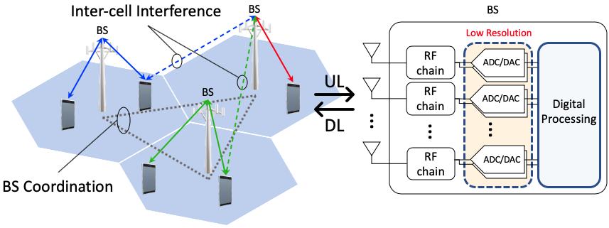
Figure 1: Multicell multiuser-MIMO configuration with low-resolution ADCs and DACs at the base station (BS).

Coordinated multipoint (CoMP) has been explored to increase throughput, coverage and reliability [14, 15, 13, 8]. In [14], CoMP beamforming (BF) and power control (PC) in uplink (UL) were presented. Considering downlink (DL) as a virtual UL, UL-DL CoMP BF and PC were further proposed in [15] in a distributed manner using local measurements. The authors in [13] showed Lagrangian-based duality for multiuser MIMO systems and proposed a distributed method to lower computational load on users and BSs. CoMP BF and PC were also studied for coarsely quanitized massive MIMO systems, and their closed-form solution and extension to a wideband scenario were investigated [8]. The synergy between massive MIMO and CoMP is studied with higher throughput [16].

In this paper, we design CoMP-based BF with the per-antenna power constraint in coarsely quantized large-scale MIMO systems. We first formulate the DL antenna power minimax problem with individual signal-to-interference-plus-noise-ratio (SINR) constraints. We then derive the Lagrangian dual of the DL problem which can be considered as a virtual UL problem with uncertain noise covariance matrices. By transforming the DL problem to a strictly feasible second-order cone program (SOCP), we derive strong duality between the DL problem and its dual. Leveraging strong duality, we propose an iterative algorithm to solve the dual in a distributed manner for fixed noise covariance matrices. The solutions of the dual are used to obtain an optimal DL BF. The optimal DL solutions update the noise covariance matrices which are then projected onto the feasible constraint set.

Notation: $\bf{A}$ is a matrix and $\bf{a}$ is a column vector. $\mathbf{A}^{H}$ and $\mathbf{A}^{T}$ denote conjugate transpose and transpose. $[{\bf A}]_{i,:}$ and $\mathbf{a}_{i}$ indicate the $i$th row and column vectors of $\bf A$. We denote $a_{i,j}$ as the $\{i,j\}$th element of $\bf A$ and $a_{i}$ as the $i$th element of $\bf a$. $\mathcal{CN}(\mu,\sigma^{2})$ is a complex Gaussian distribution with mean $\mu$ and variance $\sigma^{2}$. The diagonal matrix $\rm diag(\bf A)$ has $\{a_{i,i}\}$ as its diagonal entries, and $\rm diag(\bf a)$ or $\rm diag({\bf a}^{T})$ has $\{a_{i}\}$ as its diagonal entries. A block diagonal matrix is presented as ${\rm blkdiag}({\bf A}_{1},\dots,{\bf A}_{N})$. ${\bf I}_{N}$ is a $N\times N$ identity matrix and ${\bf 1}_{N}$ is a $N\times 1$ ones vector. $\otimes$ represents Kronecker product.

II System Model

We consider a multicell multiuser-MIMO network with $N_{c}$ cells, $N_{u}$ single-antenna users per cell. BS_i represents the BS with $N_{b}$ antennas in cell $i$ that serves $N_{u}$ dedicated users. We assume that the BSs distributed over $N_{c}$ cells cooperate and employ low-resolution DACs.

II-A DL System Models with Low-Resolution DACs

Let ${\bf s}_{i}\!\in\!\mbox{$\mathbb{C}$}^{N_{u}}$ denote the symbols for $N_{u}$ users in cell $i$ and ${\bf W}_{i}\!=\!\left[{\bf w}_{i,1},\ldots,{\bf w}_{i,N_{c}}\right]\!\in\!\mbox{$\mathbb{C}$}^{N_{b}\times N_{u}}$ collects the associated precoders. We define the precoded signals as ${\bf x}_{i}={\bf W}_{i}{\bf s}_{i}$. Upon generating ${\bf x}_{i}$, the signal is treated by the low-resolution DACs with $b$ quantization bits. For analytic tractability, we adopt the AQNM [8, 17] that delivers a linear approximation of the quantization process derived from assuming a scalar minimum-mean-squared-error (MMSE) quantizer. Under the AQNM, the quantized signal is modeled as

$${\bf x}_{{\rm q},i}=\alpha{\bf x}_{i}+{\bf q}_{i}$$ (1)

where ${\bf q}_{i}\sim\mbox{$\mathcal{C}$}\mbox{$\mathcal{N}$}({\bf 0},{\bf C}_{{\bf q}_{i}{\bf q}_{i}})$ is the quantization noise vector at BS_i with its covariance matrix of [8]

$${\bf C}_{{\bf q}_{i}{\bf q}_{i}}=\alpha\beta{\rm diag}\big{(}{\bf W}_{i}{\bf W}_{i}^{H}\big{)}.$$ (2)

The quantization gain $\alpha$ is defined as $\alpha\!=\!1-\beta$ where $\beta$’s are listed in Table 1 in [18] for $b\leq 5$ assuming ${\bf s}_{i}\!\sim\!\mathcal{CN}({\bf 0}_{N_{u}},{\bf I}_{N_{u}}),\forall i\in\{1,\ldots,N_{c}\}$.

Due to the broadcast channel, users in cell $i$ receive signals from all BSs. By defining ${\bf H}_{i,j}$ as the channel between BS_i and users in cell $j$, the received signal at user $u$ in cell $i$ is

$$y_{i,u}\!=\!\ \alpha{\bf h}_{i,i,u}^{H}\!{\bf w}_{i,u}{s}_{i,u}$$

$$+\alpha\!\!\!\!\!\!\sum_{(j,v)\neq(i,u)}^{(N_{c},N_{u})}\!\!\!\!{\bf h}_{j,i,v}^{H}\!{\bf w}_{j,v}{s}_{j,v}\!+\!\sum_{j=1}^{N_{c}}{\bf h}_{j,i,u}^{H}{\bf q}_{j}\!+\!n_{i,u}$$ (3)

where the DL channel between BS_j and user $u$ in cell $i$ is ${\bf h}^{H}_{j,i,u}$, and $n_{i,u}\sim\mathcal{CN}(0,1)$. Based on (2) and (3) the DL SINR for user $u$ in cell $i$ is expressed as

$$\Gamma_{i,u}=\frac{\alpha^{2}|{\bf h}_{i,i,u}^{H}{\bf w}_{i,u}|^{2}}{\alpha^{2}\sum_{(j,v)\neq(i,u)}^{N_{c},N_{u}}\!|{\bf h}_{j,i,u}^{H}{\bf w}_{j,v}|^{2}+{\rm Q}_{i,u}+\!\sigma^{2}}$$ (4)

with the quantization noise terms of

$${\rm Q}_{i,u}=\sum_{j=1}^{N_{c}}{\bf h}_{j,i,u}^{H}{\bf C}_{{\bf q}_{j},{\bf q}_{j}}{\bf h}_{j,i,u}.$$ (5)

Finally, the DL transmit power minimization problem with per-antenna power constraints is formulated as

$$\mathop{{\text{minimize}}}_{{\bf w}_{i,u},\ p_{\rm 0}} \;\;p_{\rm 0}$$ (6)

subject to $$\;\;\Gamma_{i,u}\geq\gamma_{i,u}$$ (7)

$$\ \Big{[}\mbox{$\mathbb{E}$}[{\bf x}_{{\rm q},i}{\bf x}_{{\rm q},i}^{H}]\Big{]}_{m,m}\leq p_{\rm 0}$$ (8)

$$\;\;\forall i,u,m.$$

Since directly solving the above problem is difficult, we first derive a Lagrangian dual and solve the problem in the dual space with a more efficient solver.

II-B Lagrangian Dual Problem

Let us collect Lagrangian multipliers as ${\boldsymbol{\Lambda}}={\rm blkdiag}\big{(}{\boldsymbol{\Lambda}}_{1},\dots,{\boldsymbol{\Lambda}}_{N_{c}}\big{)}$ where ${\boldsymbol{\Lambda}}_{i}={\rm diag}\big{(}\lambda_{i,1},\dots,\lambda_{i,N_{u}}\big{)}$. In Theorem 1, a virtual UL problem is derived as a dual problem of (6).

Theorem 1 (Duality).

The Lagrangian dual problem of the DL problem in (6) is equivalent to

$$\max_{{\bf D}_{i}}\min_{\lambda_{i,u}} \;\;\sum_{i,u}^{N_{c},N_{u}}\lambda_{i,u}\sigma^{2}$$ (9)

subject to $$\;\;\max_{{\bf f}_{i,u}}\hat{\Gamma}_{i,u}\geq\gamma_{i,u},$$ (10)

$$\;\;{\bf D}_{i}\succeq 0,\ {\bf D}_{i}\in\mbox{$\mathbb{R}$}^{N_{b}\times N_{b}}:\text{\rm diagonal},$$ (11)

$$\;\;{\rm tr}({\bf D}_{i})\leq N_{b}\quad\forall i,u$$ (12)

with UL SINR of

$$\hat{\Gamma}_{i,u}\!=\!\frac{\alpha^{2}\lambda_{i,u}|{\bf f}_{i,u}^{H}{\bf h}_{i,i,u}|^{2}}{{\bf f}_{i,u}^{H}{\bf Z}_{i,u}{\bf f}_{i,u}}$$ (13)

where

$${\bf Z}_{i,u}= \alpha^{2}\!\!\!\!\!\!\!\sum_{(j,v)\neq(i,u)}\!\!\!\!\!\!\!\lambda_{j,v}{\bf h}_{i,j,v}{\bf h}_{i,j,v}^{H}$$

$$+\alpha^{2}{{\bf D}_{i}}+\alpha\beta{\rm diag}({\bf H}_{i}{\boldsymbol{\Lambda}}{\bf H}_{i}^{H}\!+\!{\bf D}_{i}).$$ (14)

Proof.

Considering ${\bf f}_{i,u}$ as a combiner for user $u$ in cell $i$, we let ${\bf f}_{i,u}$ be the MMSE equalizer as

$${\bf f}_{i,u}= {\bf Z}_{i,u}^{-1}{\bf h}_{i,i,u}.$$ (15)

With the MMSE combiner that maximizes $\hat{\Gamma}_{i,u}$, (10) is simplified as

$$\max_{{{\bf D}}_{i}}\min_{\lambda_{i,u}} \;\;\sum_{i,u}^{N_{c},N_{u}}\lambda_{i,u}\sigma^{2}$$ (16)

subject to $$\;\;{\bf K}_{i}({\boldsymbol{\Lambda}})\preceq\alpha\left(1+\frac{1}{\gamma_{i,u}}\right)\lambda_{i,u}{\bf h}_{i,i,u}{\bf h}_{i,i,u}^{H},$$ (17)

$$\;\;{\bf D}_{i}\succeq 0,\ {\bf D}_{i}\in\mbox{$\mathbb{R}$}^{N_{b}\times N_{b}}:\text{\rm diagonal},$$

$$\;\;{\rm tr}({\bf D}_{i})\leq N_{b}\quad\forall i,u$$

where

$${\bf K}_{i}({\boldsymbol{\Lambda}})\!=\!{\bf D}_{i}\!+\!\alpha\!\sum_{j,v}\!\lambda_{j,v}{\bf h}_{i,j,v}{\bf h}_{i,j,v}^{H}\!+\!\beta{\rm diag}\Big{(}{\bf H}_{i}{\boldsymbol{\Lambda}}{\bf H}_{i}^{H}\Big{)},$$ (18)

which is the covariance matrix of the received signal at BS_i.

Now, we show that (16) is equivalent to the Lagrangian dual of (6). The per-antenna constraint in (8) is rewritten as

$$\Big{[}\mbox{$\mathbb{E}$}[{\bf x}_{{\rm q},i}{\bf x}_{{\rm q},i}^{H}]\Big{]}_{m,m}=\left[\alpha{\bf W}_{i}{\bf W}_{i}^{H}\right]_{m,m}.$$ (19)

We replace the objective function in (6) with $N_{c}N_{b}p_{\rm 0}$ that does not affect the problem. With Lagrangian multipliers $\lambda_{i,u}$ and $\mu_{i,m}$, the Lagrangian of (6) is then given as

$${\mbox{$\mathcal{L}$}}\!=\! \,N_{c}N_{b}p_{\rm 0}\!-\!\!\sum_{i,u}\!\lambda_{i,u}\Bigg{(}\!\frac{\alpha^{2}|{\bf w}_{i,u}^{H}{\bf h}_{i,i,u}|^{2}}{\gamma_{i,u}}\!-\alpha^{2}\!\!\!\!\!\!\!\!\sum_{(j,v)\neq(i,u)}^{N_{c},N_{u}}\!\!\!\!\!\!\!|{\bf h}_{j,i,u}^{H}{\bf w}_{j,v}|^{2}$$

$$\!-\!{\rm Q}_{i,u}\!-\!\sigma^{2}\!\Bigg{)}+\sum_{i,m}\mu_{i,m}\left(\left[\alpha{\bf W}_{i}{\bf W}_{i}^{H}\right]_{m,m}-p_{\rm 0}\right).$$ (20)

First, from the proof of Theorem 2 in [8], we have $\sum_{i,u}\lambda_{i,u}{\rm Q}_{i,u}$ in (20) rewritten as

$$\sum_{i,u}\lambda_{i,u}{\rm Q}_{i,u}=\alpha\beta\sum_{i,u}\!{\bf w}_{i,u}^{H}{\rm diag}\left({\bf H}_{i}{\boldsymbol{\Lambda}}{\bf H}_{i}^{H}\!\right)\!{\bf w}_{i,u}.$$ (21)

Next, we let ${\bf D}_{i}={\rm diag}(\mu_{i,1},\dots,\mu_{i,N_{b}})$. We can cast $\sum_{i,m}\mu_{i,m}\left[\alpha{\bf W}_{i}{\bf W}_{i}^{H}\right]_{m,m}$ in (20) to

$$\sum_{i,m}\mu_{i,m}\bigg{[}\sum_{u}{\bf w}_{i,u}{\bf w}_{i,u}^{H}\bigg{]}_{m,m}\! =\sum_{i,m}\sum_{u}w^{*}_{i,u,m}\mu_{i,m}w_{i,u,m}$$

$$=\sum_{i,u}{\bf w}^{H}_{i,u}{\bf D}_{i}{\bf w}_{i,u}$$ (22)

where $w_{i,u,m}$ denotes $m$th element of ${\bf w}_{i,u}$. Lastly, $\sum_{i,m}\mu_{i,m}p_{\rm 0}$ can be rewritten as

$$p_{\rm 0}\sum_{i,m}\mu_{i,m}=p_{\rm 0}\sum_{i=1}^{N_{c}}{\rm tr}({\bf D}_{i}).$$ (23)

Applying (21), (22), and (23) to the Lagrangian in (20), we finally have the reformed Lagrangian as

$${\mbox{$\mathcal{L}$}}\!=\! \sum_{i,u}\lambda_{i,u}\sigma^{2}\!-\!p_{\rm 0}\!\sum_{i}\!\big{[}{\rm tr}({\bf D}_{i})\!-\!N_{b}\big{]}\!$$ (24)

$$+\!\sum_{i,u}\!{\bf w}_{i,u}^{H}\!\bigg{(}\alpha{\bf D}_{i}\!-\!\alpha^{2}\!\left(\!1\!+\!\frac{1}{\gamma_{i,u}}\!\right)\!\lambda_{i,u}{\bf h}_{i,i,u}{\bf h}_{i,i,u}^{H}$$

$$+\alpha^{2}\!\sum_{j,v}\lambda_{j,v}{\bf h}_{i,j,v}{\bf h}_{i,j,v}^{H}\!+\!\alpha\beta{\rm diag}\!\left({\bf H}_{i}\,{\boldsymbol{\Lambda}}\,{\bf H}_{i}^{H}\!\right)\!\bigg{)}{\bf w}_{i,u}.$$

Let the dual objective function be $g({\bf D}_{i},\lambda_{i,u})=\min_{{\bf w}_{i,u},p_{\rm 0}}\mathcal{L}$. We then need ${\rm tr}({\bf D}_{i})\leq N_{b}$ and ${\bf K}_{i}({\boldsymbol{\Lambda}})\succeq\alpha\big{(}1+1/{\gamma_{i,u}}\big{)}\lambda_{i,u}{\bf h}_{i,i,u}{\bf h}_{i,i,u}^{H}$, where ${\bf K}_{i}({\boldsymbol{\Lambda}})$ is in (18). Consequently, the Lagrangian dual problem of (6) becomes

$$\max_{{{\bf D}}_{i}}\max_{\lambda_{i,u}} \;\;\sum_{i,u}^{N_{c},N_{u}}\lambda_{i,u}\sigma^{2}$$ (25)

subject to $$\;\;{\bf K}_{i}({\boldsymbol{\Lambda}})\succeq\alpha\bigg{(}1+\frac{1}{\gamma_{i,u}}\bigg{)}\lambda_{i,u}{\bf h}_{i,i,u}{\bf h}_{i,i,u}^{H},$$ (26)

$$\;\;{\bf D}_{i}\succeq 0,\ {\bf D}_{i}\in\mbox{$\mathbb{R}$}^{N_{b}\times N_{b}}:\text{\rm diagonal},$$

$$\;\;{\rm tr}({\bf D}_{i})\leq N_{b}\quad\forall i,u$$

We note that the differences between the problem in (16) and in (25) are the reversed objectives with respect to $\lambda_{i,u}$ (i.e., $\min$ vs. $\max$) and reversed SINR inequalities in (17) and (26). Since the problems in (16) and (25) have optimal solutions when the SINR constraints are active, the solutions for the problems are indeed equivalent to each other with the active SINR constraints. ∎

We remark that $\hat{\Gamma}_{i,u}$ in (13) can be interpreted as the SINR of user $u$ in cell $i$ for the UL system with low-resolution ADCs, i.e., ${\bf f}_{i,u}$ is a combiner for user $u$ in cell $i$, $\lambda_{i,u}$ is transmit power for user $u$ in cell $i$, ${\bf C}_{i}$ is an aggregated quantization noise of BS_i after quantization, and ${\bf D}_{i}$ is a diagonal matrix of noise variances at the antennas of BS_i with uncertain noise covariance in UL direction. Accordingly, the Lagrangian dual problem is considered to be an antenna power minimax problem with noise variance constraints for a virtual UL system with low-resolution ADCs at the BSs.

Corollary 1 (Strong Duality).

Zero duality gap exists between the DL formulation and its associated dual.

Proof.

The primal DL problem is rewritten as

$$\min_{{{\bf W}},P_{o}}p_{o}$$ (27)

$${\rm s.t.}\ \Gamma_{i,u}\geq\gamma_{i,u},\quad\forall i,u$$ (28)

$$\left[\alpha{\bf W}_{i}{\bf W}_{i}^{H}\right]_{m,m}\leq p_{o}$$ (29)

Let ${\bf W}_{\rm BD}\!=\!{\rm blkdiag}({\bf W}_{1},\dots,{\bf W}_{N_{c}})$, $\tilde{{\bf W}}_{\rm BD}\!=\!{\rm blkdiag}(({\bf I}_{N_{b}}\otimes{\bf W}_{1}),\dots,({\bf I}_{N_{b}}\otimes{\bf W}_{N_{c}}))$, ${\bf E}_{j,i,u}\!=\!{\rm diag}({\bf h}_{j,i,u}{\bf h}_{j,i,u}^{H})$, and $\mbox{$\mathbb{E}$}_{i,u}\!=\!{\rm vec}({\bf E}^{1/2}_{1,i,u},\ldots,{\bf E}^{1/2}_{N_{c},i,u})$. The SINR constraints in (28) can be rewritten as

$$\alpha^{2}\bigg{(}1+\frac{1}{\gamma_{i,u}}\bigg{)}|{\bf w}_{i,u}^{H}{\bf h}_{i,i,u}|^{2}$$ (30)

$$\geq\left\|\begin{matrix}\alpha{\bf W}_{\rm BD}^{H}{\rm vec}({\bf h}_{1,i,u},\dots,{\bf h}_{N_{c},i,u})\\ \sqrt{\alpha\beta}\tilde{{\bf W}}_{\rm BD}\mbox{$\mathbb{E}$}_{i,u}\\ \sigma\end{matrix}\right\|^{2}$$ (31)

for all $i$, $u$, and $k$. In addition, the per-antenna constraint in (29) is rewritten as

$$\left[\alpha{\bf W}_{i}{\bf W}_{i}^{H}\right]_{m,m}=\alpha\|{\bf e}_{m}^{H}{\bf W}_{i}\|^{2}$$ (32)

for all $m$ which is a convex constraint. Accordingly, we eventually have the standard SOCP form. Next, (6) is strictly feasible because, for a given solution ${\bf W}$, it can be scaled by a factor of $c>1$ satisfying the constraints. Thus, strong duality holds between (6) and (9). ∎

Corollary 2.

An optimal DL precoder forms a linear relationship with the UL MMSE receiver, i.e., ${\bf w}_{i,u}=\sqrt{{\tau}_{i,u}}{\bf f}_{i,u}\;\forall i,u$. Here, ${\tau}_{i,u}$ is derived from solving ${\boldsymbol{\tau}}={\boldsymbol{\Sigma}}^{-1}{\bf 1}$, where ${\bf 1}$ is a $N_{u}N_{c}\times 1$ column vector, ${\boldsymbol{\tau}}=[{\boldsymbol{\tau}}_{1}^{T},{\boldsymbol{\tau}}_{2}^{T},\cdots,{\boldsymbol{\tau}}_{N_{c}}^{T}]^{T}$ and ${\boldsymbol{\tau}}_{i}^{T}=[{\tau}_{i,1},{\tau}_{i,2},\cdots,{\tau}_{i,N_{u}}]^{T}$, and ${\boldsymbol{\Sigma}}$ is defined as

$${\boldsymbol{\Sigma}}=\begin{pmatrix}{\boldsymbol{\Sigma}}_{1,1}&{\boldsymbol{\Sigma}}_{1,2}&\cdots&{\boldsymbol{\Sigma}}_{1,N_{c}}\\ {\boldsymbol{\Sigma}}_{2,1}&{\boldsymbol{\Sigma}}_{2,2}&\cdots&{\boldsymbol{\Sigma}}_{2,N_{c}}\\ \vdots&\vdots&\ddots&\vdots\\ {\boldsymbol{\Sigma}}_{N_{c},1}&{\boldsymbol{\Sigma}}_{N_{c},2}&\cdots&{\boldsymbol{\Sigma}}_{N_{c},N_{c}}\end{pmatrix},$$ (33)

and

$$[{\boldsymbol{\Sigma}}_{i,j}]_{u,v}$$

$$=\begin{cases}\frac{\alpha^{2}}{\gamma_{i,u}}|{\bf h}_{i,i,u}^{H}{\bf f}_{i,u}|^{2}\!-\alpha(1\!-\!\alpha){\bf f}_{i,u}^{H}{\rm diag}\big{(}{\bf h}_{i,i,u}{\bf h}_{i,i,u}^{H}\!\big{)}{\bf f}_{i,u}\\ \text{if }i=j\text{, }u=v,\\ -\alpha^{2}|{\bf h}_{j,i,u}^{H}{\bf f}_{j,v}|^{2}\!-\alpha(1\!-\!\alpha){\bf f}_{j,v}^{H}{\rm diag}\big{(}{\bf h}_{j,i,u}{\bf h}_{j,i,u}^{H}\!\big{)}{\bf f}_{j,v}\\ \text{otherwise.}\end{cases}$$

Proof.

Starting from the Lagrangian in (24), we find the derivative of the Lagrangian regarding ${\bf w}_{i,u}$ as

$$2\bigg{(}\alpha{\bf D}_{i}\!-\!\alpha^{2}\!\left(\!1\!+\!\frac{1}{\gamma_{i,u}}\!\right)\!\lambda_{i,u}{\bf h}_{i,i,u}{\bf h}_{i,i,u}^{H}$$ (34)

$$+\alpha^{2}\!\sum_{j,v}\lambda_{j,v}{\bf h}_{i,j,v}{\bf h}_{i,j,v}^{H}+\!\alpha(1-\alpha){\rm diag}\!\left({\bf H}_{i}\,{\boldsymbol{\Lambda}}\,{\bf H}_{i}^{H}\!\right)\!\bigg{)}{\bf w}_{i,u}.$$

We then set the derivative to zero, and solve it for ${\bf w}_{i,u}$ as

$${\bf w}_{i,u}=\bigg{(}\!\alpha^{2}\!\!\!\!\!\sum_{(j,v)\neq(i,u)}\!\!\!\lambda_{j,v}{\bf h}_{i,j,v}{\bf h}_{i,j,v}^{H}\!$$

$$+\!\alpha(1\!-\!\alpha){\rm diag}\!\left({\bf H}_{i}{\boldsymbol{\Lambda}}{\bf H}_{i}^{H}\!\right)\!+\!\alpha{\bf D}_{i}\!\bigg{)}^{\!-1}\!\!\frac{\alpha^{2}}{\gamma_{i,u}}\!\lambda_{i,u}{\bf h}_{i,i,u}{\bf h}_{i,i,u}^{H}{\bf w}_{i,u}$$

$$=\frac{\alpha^{2}}{\gamma_{i,u}}\lambda_{i,u}{\bf h}_{i,i,u}^{H}{\bf w}_{i,u}{\bf f}_{i,u}$$

where ${\bf f}_{i,u}$ is in (15) and the last equality is valid because ${\bf h}_{i,i,u}^{H}{\bf w}_{i,u}$ is a scalar. Accordingly, we can justify the form of ${\bf w}_{i,u}=\sqrt{\tau_{i,u}}{\bf f}_{i,u}$ with properly designed $\tau_{i,u}$.

To satisfy the KKT stationarity condition with the DL constraint in (7), $\Gamma_{i,u}$ has to meet the target SINR constraint with equality. Since the DL precoder is deeply embedded in the quantization noise term, i.e., ${\rm Q}_{i,u}$, in the DL SINR expression, we first simplify ${\rm Q}_{i,u}$. Let us define $\mu_{i^{\prime},u^{\prime}}$ where $\mu_{i^{\prime},u^{\prime}}=1$ if $i^{\prime}=i$ and $u^{\prime}=u$, and $\mu_{i^{\prime},u^{\prime}}=0$ otherwise. To compose the DL constraint in a tractable form, we can rewrite the quantization error term in (4) as

$${\rm Q}_{i,u} \stackrel{{\scriptstyle(a)}}{{=}}\!\alpha\beta\sum_{j=1}^{N_{c}}{\bf h}_{j,i,u}^{H}{\rm diag}\big{(}\mbox{${\bf{W}}$}_{j}\mbox{${\bf{W}}$}_{j}^{H}\big{)}{\bf h}_{j,i,u}\!$$

$$=\alpha\beta\sum_{i^{\prime},u^{\prime},j}\mu_{i^{\prime},u^{\prime}}{\bf h}_{j,i^{\prime},u^{\prime}}^{H}{\rm diag}\big{(}\mbox{${\bf{W}}$}_{j}\mbox{${\bf{W}}$}_{j}^{H}\big{)}{\bf h}_{j,i^{\prime},u^{\prime}}$$

$$=\alpha\beta\sum_{j,v}{\bf w}_{j,v}^{H}{\rm diag}\left({\bf H}_{j}\,\mbox{${\bf{M}}$}\,{\bf H}_{j}^{H}\right)\!{\bf w}_{j,v}$$

$$\stackrel{{\scriptstyle(b)}}{{=}}\alpha\beta\sum_{j,v}{\bf w}_{j,v}^{H}{\rm diag}\left({\bf h}_{j,i,u}{\bf h}_{j,i,u}^{H}\!{}^{H}\!\right)\!{\bf w}_{j,v}^{H},$$ (35)

where $(a)$ is obtained by plugging (2) into (5). We define ${\bf M}_{i}\!=\!{\rm diag}(\mu_{i,1},\dots,\mu_{i,N_{u}})$ and ${{\bf M}}\!=\!{\rm blkdiag}({{\bf M}}_{1},\dots,{{\bf M}}_{N_{c}})$. By the definition of ${\bf M}$, $(b)$ is from ${\bf H}_{j}\,\mbox{${\bf{M}}$}\,{\bf H}_{j}^{H}={\bf h}_{j,i,u}{\bf h}_{j,i,u}^{H}$.

Accordingly, we can create the DL SINR constraints with equality as follows:

$$\sigma^{2} =\frac{\alpha^{2}}{\gamma_{i,u}}|{\bf h}_{i,i,u}^{H}{\bf w}_{i,u}|^{2}-\alpha^{2}\!\!\!\!\sum_{(j,v)\neq(i,u)}^{N_{c},N_{u}}\!|{\bf h}_{j,i,u}^{H}{\bf w}_{j,v}|^{2}-{\rm Q}_{i,u}$$

$$\stackrel{{\scriptstyle(a)}}{{=}}\frac{\alpha^{2}}{\gamma_{i,u}}|{\bf h}_{i,i,u}^{H}{\bf f}_{i,u}|^{2}\tau_{i,u}-\alpha^{2}\!\!\!\!\!\!\!\sum_{(j,v)\neq(i,u)}\!\!\!\!\!{|{\bf h}_{j,i,u}{\bf f}_{j,v}^{H}|^{2}}\tau_{j,v}\!$$

$$\quad-\!\alpha\beta\!\sum_{j,v}\!{\bf w}_{j,v}^{H}{\rm diag}\!\left({\bf h}_{j,i,u}{\bf h}_{j,i,u}^{H}\!{}^{H}\right)\!{\bf w}_{j,v}^{H},$$ (36)

for all $i$, $u$ where $(a)$ is from (35) and ${\bf w}_{i,u}=\sqrt{\tau_{i,u}}{\bf f}_{i,u}$. Combining (36) for all $i,u$ gives a system of linear equations as $\sigma^{2}{\bf 1}={\boldsymbol{\Sigma}}{\boldsymbol{\tau}}$, thereby having $\tau_{i,u}$ through ${\boldsymbol{\tau}}=\sigma^{2}{\boldsymbol{\Sigma}}^{-1}{\bf 1}$. ∎

II-C Distributed Iterative Algorithm

In this subsection, we characterize solutions by exploiting strong duality and further adopt the fixed-point iteration with a subgradient projection method [13].

Corollary 3.

For a fixed ${\bf D}_{i}$, the optimal power for the uplink total power minimization problem in (9) is given as

$$\lambda_{i,u}=\frac{1}{\alpha\left(1+\frac{1}{\gamma_{i,u}}\right){\bf h}_{i,i,u}^{H}{\bf K}_{i}^{-1}({\boldsymbol{\Lambda}}){\bf h}_{i,i,u}},$$ (37)

where ${\bf K}_{i}({\boldsymbol{\Lambda}})$ is defined in (18).

Proof.

Setting (34) to zero and solving it for $\lambda_{i,u}$ produce (37). The solution of $\lambda_{i,u}$ then satisfies the stationary condition, and we further observe that the UL SINR constraint in (8) is active at the solution satisfying the complementary slackness condition. Therefore, (37) is optimal solution of the virtual UL problem. ∎

The UL power control solution from Corollary 3 is fundamentally designed for the subproblem of (9) written as

$$f\!\left({\bf D}_{i}\right)= \min_{\lambda_{i,u}}\;\;\sum_{i,u}^{N_{c},N_{u}}\lambda_{i,u}\sigma^{2}$$ (38)

$${\text{ \rm subject to}}\;\;\max_{{\bf f}_{i,u}}\hat{\Gamma}_{i,u}\geq\gamma_{i,u}\;\;\forall i,u,$$

which is the inner optimization on $\lambda_{i,u}$ of $g({\bf D}_{i},\lambda_{i,u})$ when MMSE filter in (15) is used for ${\bf f}_{i,u}$. However, the solutions do not guarantee a global optimum over the entire feasible candidates of ${\bf D}_{i}$ in (11)-(12). Therefore, as a second stage, the external loop on ${\bf D}_{i}$ is needed. We then use a projected subgradient ascend method to maximize the objective function while satisfying the constraint on ${\bf D}_{i}$. Note that $f\!\left({\bf D}_{i}\right)$ is concave in ${\bf D}_{i}$ since the Lagrangian function in $\eqref{eq:lagrangian}$ is affine in $\lambda$ and $\mu$, and the infimum of affine functions is still concave.

Corollary 4 (Subgradient).

${\rm diag}\left(\sum_{u}{\bf w}_{i,u}{\bf w}_{i,u}^{H}\right)$ is a subgradient of (38) in updating ${\bf D}_{i}$.

Proof.

Using strong duality between UL and DL, the UL subproblem $f\!\left({\bf D}_{i}\right)$ in (38) for a fixed ${\bf D}_{i}$ is equivalent to

$$f\!\left({\bf D}_{i}\right)= \min_{{\bf w}_{i,u}}\;\;\sum_{u}^{N_{u}}{\bf w}_{i,u}^{H}{\bf D}_{i}{\bf w}_{i,u}$$ (39)

$${\text{ \rm subject to}}\;\;\Gamma_{i,u}\geq\gamma_{i,u}\;\;\forall i,u,$$

based on the proof of Theorem 1. We introduce two arbitrary diagonal covariance matrices ${\bf D}_{i}$ and ${\bf D}_{i}^{\prime}$ whose associated optimal beamformer is ${\bf w}_{i,u}$ and ${\bf w}_{i,u}^{\prime}$, respectively. We then derive a subgradient as follows:

$$f\!\left({\bf D}_{i}^{\prime}\right)-f\!\left({\bf D}_{i}\right)=\sum_{u}{\bf w}_{i,u}^{{}^{\prime}H}{\bf D}_{i}^{\prime}{\bf w}_{i,u}^{\prime}-\sum_{u}{\bf w}_{i,u}^{H}{\bf D}_{i}{\bf w}_{i,u}$$ (40)

$$\qquad\qquad\qquad\;\;\leq\sum_{u}{\bf w}_{i,u}^{H}{\bf D}_{i}^{\prime}{\bf w}_{i,u}-\sum_{u}{\bf w}_{i,u}^{H}{\bf D}_{i}{\bf w}_{i,u}$$ (41)

$$\qquad\qquad={\rm tr}\left({\rm diag}\left(\sum_{u}{\bf w}_{i,u}{\bf w}_{i,u}^{H}\right)\left({\bf D}_{i}^{\prime}-{\bf D}_{i}\right)\right).$$ (42)

By the definition of subgradients, the multiplier in front of ${\bf D}_{i}^{\prime}-{\bf D}_{i}$ becomes a subgradient of $f({\bf D}_{i})$. ∎

We finally plug the subproblem into the entire DL problem in (9). Recall that the main target is to maximize $f({\bf D}_{i})$ while satisfying the constraints on ${\bf D}_{i}$. After obtaining a converged solution of (38) for a fixed ${\bf D}_{i}$, we take a step in the direction of a positive subgradient. We further project the updated ${\bf D}_{i}$ onto the feasible set on ${\bf D}_{i}$ in (11) and (12) because the updated ${\bf D}_{i}$ probably violates the feasible domain. The complete algorithm is summarized in Algorithm 1.

1 Initialize $\lambda_{i,u}$, $\forall i,u$ and ${\bf D}_{i}^{(0)}$, $\forall i$.

2 while ${\bf D}_{i}^{(n)}$’s do not converge do

3       Iteratively update $\lambda_{i,u}$ until converges as

$$\lambda_{i,u}=\frac{1}{\alpha\Big{(}1+\frac{1}{\gamma_{i,u}}\Big{)}{\bf h}_{i,i,u}^{H}\left[{\bf K}_{i}^{(n)}({\boldsymbol{\Lambda}})\right]^{-1}{\bf h}_{i,i,u}},$$

for all $i,u$ where ${\bf K}_{i}^{(n)}({\boldsymbol{\Lambda}})$ is updated according to (18) using $\lambda_{i,u}$ and ${\bf D}_{i}^{(n)}$.

4       Find the UL MMSE equalizer ${\bf f}_{i,u}$ in (15) with ${\bf D}_{i}^{(n)}$ and the converged $\lambda_{i,u}$

5       Compute the DL precoder ${\bf w}_{i,u}$ from Corollary 2.

6       for $i=1$ to $N_{c}$ do

7             ${\bf D}_{i}^{(n+1)}\!\leftarrow\!{\bf D}_{i}^{(n)}\!+\!\eta\;{\rm diag}\left(\sum_{u}{\bf w}_{i,u}{\bf w}_{i,u}^{H}\right)$.

8             Project ${\bf D}_{i}^{(n+1)}$ onto the feasible set (11)-(12) until converges as

9             ${\bf D}_{i}^{(n+1)}\!\leftarrow\!{\bf D}_{i}^{(n+1)}\!\!-\!\frac{\rm max\left(0,{\rm tr}\left({\bf D}_{i}^{(n+1)}\right)-N_{b}\right)}{\left\|{\bf 1}_{N_{b}}\right\|^{2}}{\bf 1}_{N_{b}}$

10      $n\leftarrow n+1$

return  ${\bf w}_{i,u}$ for all $i,u$.

Algorithm 1 Joint Power-Minimizing Transmission with Per-Antenna Constraints

III Simulation Results

We evaluate the derived results of the proposed quantization-aware iterative CoMP algorithm with per-antenna constraints (Q-iCoMP-PA) against the quantization-aware iterative CoMP algorithm (Q-iCoMP) in [8]. The former is based on the antenna power minimax problem while the latter focuses on the total transmit power minimization problem.

Each BS is in the center of own hexagonal cell and BSs operate beside each other. We assume that the small scale fading of each channel follows Rayleigh fading with zero mean and unit variance. For large scale fading, we use the log-distance pathloss model in [19]. The distance between adjacent BSs is $2\ \rm km$. The minimum distance between BS and user is $100\ \rm m$. Considering a $2.4\ \rm GHz$ carrier frequency with $10\ \rm MHz$ bandwidth, we use $8.7\ \rm dB$ lognormal shadowing variance and $5\ \rm dB$ noise figure. For simplicity, we assume an equal target SINR for all users, i.e., $\gamma_{i,u}=\gamma$ for all $i,u$.

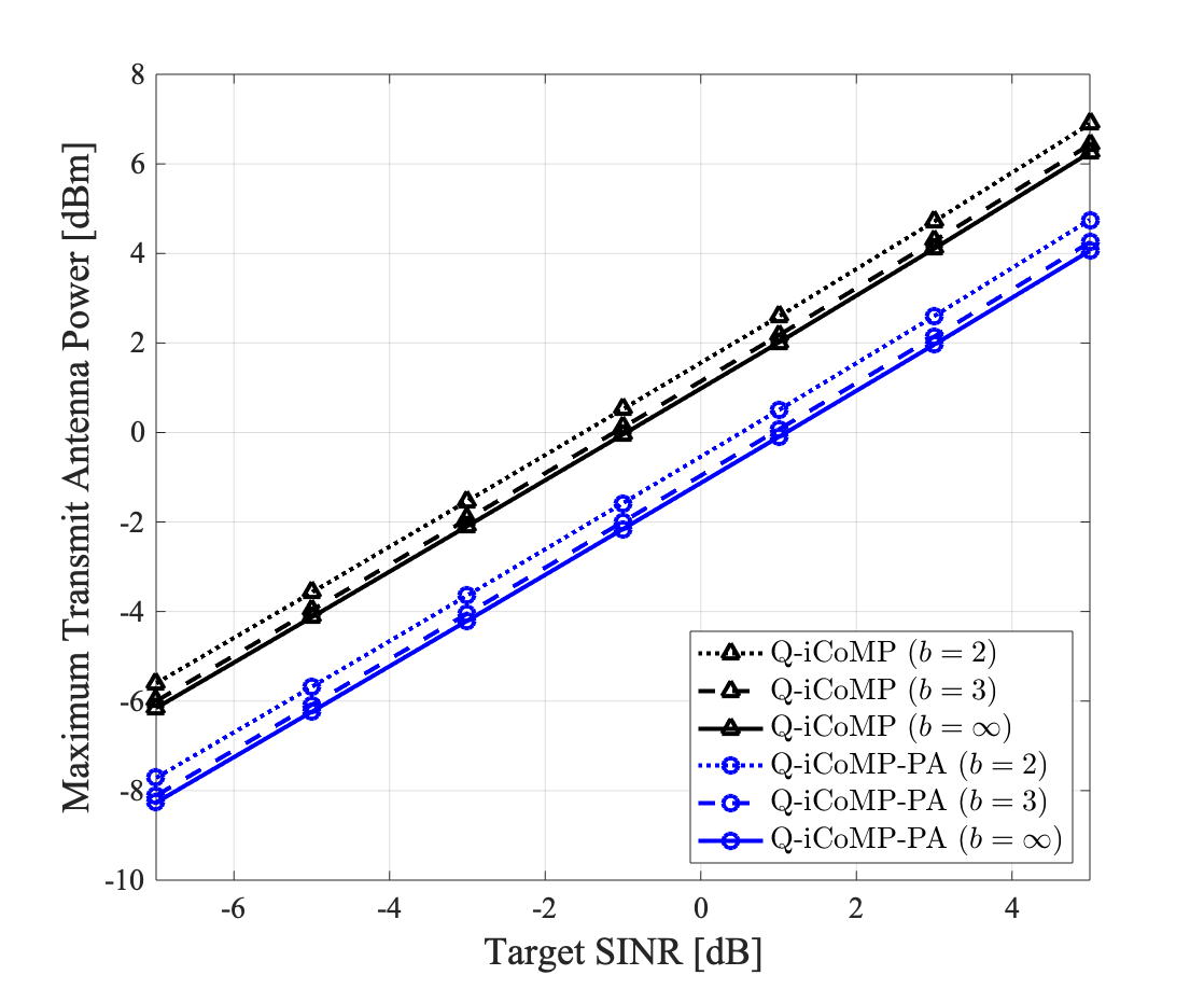
Figure 2: Maximum transmit antenna power vs. target SINR for the network with $N_{b}=32$ antennas per BS, $N_{c}=4$ cells, $N_{u}=2$ users per cell, and $b\in\{2,3,\infty\}$ bits using 20 channel realizations per target SINR value.

Fig. 2 shows maximum transmit antenna power in DL direction across all $N_{c}N_{b}$ transmit antennas for given target SINRs. We consider a communication configuration with $N_{b}=32$ BS antennas, $N_{c}=4$ cells, and $N_{u}=2$ users per cell. We test both infinite-resolution and low-resolution converters, i.e., $b\!\in\!\{2,3,\infty\}$. When using infinite-resolution ADCs and DACs, we have slightly lower peak power compared to one with 3-bit data converters, however the gap between $b=2$, $b=3$, and $b=\infty$ cases is marginal on both Q-iCoMP and Q-iCoMP-PA by properly incorporating the coarse quantization error into the design of beamformers. With multi-cell coordination, both Q-iCoMP and Q-iCoMP-PA do not suffer from implausible power consumption and undesirable divergence. However, based on the primal problem of Q-iCoMP-PA, the proposed algorithm can limit the maximum transmit power providing around 2 dB gain over the regular Q-iCoMP.

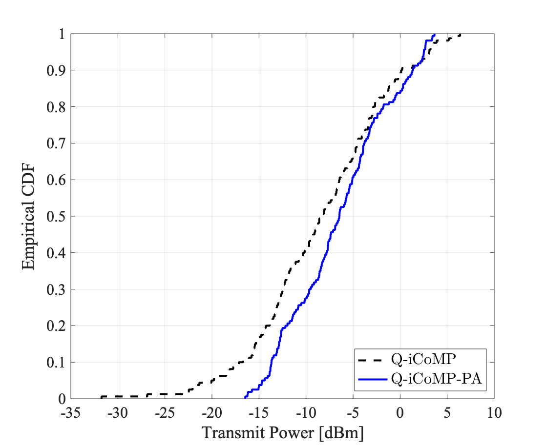
Figure 3: Empirical CDF of the transmit power of the BS antennas in the network with $N_{b}=32$ antennas per BS, $N_{c}=5$ cells, $N_{u}=2$ users per cell, $b=3$ quantization bits, and $\gamma=2\ \rm dB$ target SINR using one channel realization. Empirical CDF gives the probability of an antenna operating at or below the given transmit power.

Fig. 3 shows the cumulative density function (CDF) of the transmit power of all antennas, i.e., $N_{b}N_{c}$ antennas, considering one channel realization. We employ a network with $N_{b}=32$ BS antennas, $N_{c}=5$ cells, $N_{u}=2$ users per cell, and $b=3$ quantization bits. From the figure, the proposed algorithm reveals two main advantages: 1) maximum transmit antenna power; and 2) operating range. Since the CDF is plotted over all antennas, the rightmost point of the CDF represents the maximum transmit power. When comparing the rightmost point of two methods, Q-iCoMP-PA achieves more than $2\ \rm dB$ gain over Q-iCoMP, which corresponds to the main purpose of the proposed method. Also, the CDF gives the operating range which is defined as the gap between the leftmost and rightmost points of the CDF. Q-iCoMP-PA works with a much narrower operating range compared with Q-iCoMP, thereby increaseing efficiency of power-related components such as power amplifier.

TABLE I: Comparison of Peak-to-average power ratio (PAPR).

$\gamma$	Methods
[dB]	Q-iCoMP	Q-iCoMP-PA
2	3.81 dB	2.16 dB
-3	3.77 dB	2.09 dB

$N_{b}=32$ antennas per BS, $N_{c}=4$ cells, $N_{u}=2$ users per cell, and $b=3$ bits.

In Table. I, we further simulate the peak-to-average power ratio (PAPR) which is directly related to the efficiency of power amplifiers. We consider a network configuration with $N_{b}=16$ BS antennas, $N_{c}\in\{2,3\}$ cells, $N_{u}=2$ users per cell, and $b=3$ bits over different constraint SINRs. With two cells in the network, the Q-iCoMP-PA achieves significant reduction over the Q-iCoMP, showing more than 1.6 dB gain on average. Therefore, Q-iCoMP-PA is more favorable for mobile communication systems by properly providing multi-cell coordination and limiting the peak power of antennas.

IV Conclusion

In this paper, we investigated the CoMP solution for a multicell configuration with low-resolution data converters when employing per-antenna power constraints for more practical deployment. Considering the coarse quantization error, we derived the antenna power minimax problem and effective UL problem with uncertain noise covariance as dual problem, and further proved zero duality gap between two problems. Leveraging strong duality, we proposed the iterative algorithm that finds the optimal dual solution for a fixed covariance and used the solution to compute the optimal DL beamformer. We further update the UL noise covariance using the optimal DL solution with the projected subgradient descent method. In simulation, the proposed Q-iCoMP-PA achieves significant gain over Q-iCoMP in terms of maximum antenna power, operating range, and PAPR, thereby improving hardware efficiency. Therefore, we can emphasize the need to limit the antenna power when deploying multicell massive MIMO communication systems with low-resolution data converters.

References

- [1] T. L. Marzetta, “Noncooperative Cellular Wireless with Unlimited Numbers of Base Station Antennas,” IEEE Trans. on Wireless Commun., vol. 9, no. 11, pp. 3590–3600, 2010.
- [2] J. Choi, J. Mo, and R. W. Heath, “Near maximum-likelihood detector and channel estimator for uplink multiuser massive MIMO systems with one-bit ADCs,” IEEE Trans. Comm., vol. 64, no. 5, pp. 2005–2018, Mar. 2016.
- [3] C. Studer and G. Durisi, “Quantized massive mu-mimo-ofdm uplink,” IEEE Trans. on Commun., vol. 64, no. 6, pp. 2387–2399, 2016.
- [4] J. Choi, Y. Cho, B. L. Evans, and A. Gatherer, “Robust learning-based ML detection for massive MIMO systems with one-bit quantized signals,” in IEEE Global Commun. Conf., 2019, pp. 1–6.
- [5] Y. Cho and S.-N. Hong, “One-bit successive-cancellation soft-output (OSS) detector for uplink MU-MIMO systems with one-bit ADCs,” IEEE Access, vol. 7, pp. 27 172–27 182, 2019.
- [6] J. Choi, B. L. Evans, and A. Gatherer, “Resolution-Adaptive Hybrid MIMO Architectures for Millimeter Wave Communications,” IEEE Trans. on Signal Process., vol. PP, no. 99, pp. 1–1, 2017.
- [7] J. Choi, G. Lee, and B. L. Evans, “Two-Stage Analog Combining in Hybrid Beamforming Systems With Low-Resolution ADCs,” IEEE Trans. on Signal Process., vol. 67, no. 9, pp. 2410–2425, 2019.
- [8] J. Choi, Y. Cho, and B. L. Evans, “Quantized massive mimo systems with multicell coordinated beamforming and power control,” IEEE Transactions on Communications, vol. 69, no. 2, pp. 946–961, 2021.
- [9] L. V. Nguyen, A. Lee Swindlehurst, and D. H. N. Nguyena, “Linear and deep neural network-based receivers for massive mimo systems with one-bit adcs,” IEEE Trans. on Wireless Commun., pp. 1–1, 2021.
- [10] J. Yuan, Q. He, M. Matthaiou, T. Q. S. Quek, and S. Jin, “Toward massive connectivity for iot in mixed-adc distributed massive mimo,” IEEE Internet of Things Journal, vol. 7, no. 3, pp. 1841–1856, 2020.
- [11] S. Park, Y. Cho, and S. Hong, “Construction of 1-bit transmit signal vectors for downlink mu-miso systems: Qam constellations,” IEEE Transactions on Vehicular Technology, vol. 70, no. 10, pp. 10 065–10 076, 2021.
- [12] W. Yu and T. Lan, “Transmitter optimization for the multi-antenna downlink with per-antenna power constraints,” IEEE Trans. on Signal process., vol. 55, no. 6, pp. 2646–2660, 2007.
- [13] H. Dahrouj and W. Yu, “Coordinated beamforming for the multicell multi-antenna wireless system,” IEEE Trans. on Wireless Commun., vol. 9, no. 5, pp. 1748–1759, 2010.
- [14] F. Rashid-Farrokhi, L. Tassiulas, and K. R. Liu, “Joint optimal power control and beamforming in wireless networks using antenna arrays,” IEEE Trans. on Commun., vol. 46, no. 10, pp. 1313–1324, 1998.
- [15] F. Rashid-Farrokhi, K. R. Liu, and L. Tassiulas, “Transmit beamforming and power control for cellular wireless systems,” IEEE J. on Sel. Areas in Commun., vol. 16, no. 8, pp. 1437–1450, 1998.
- [16] V. Jungnickel, K. Manolakis, W. Zirwas, B. Panzner, V. Braun, M. Lossow, M. Sternad, R. Apelfröjd, and T. Svensson, “The role of small cells, coordinated multipoint, and massive MIMO in 5G,” IEEE Commun. Mag., vol. 52, no. 5, pp. 44–51, 2014.
- [17] O. Orhan, E. Erkip, and S. Rangan, “Low power analog-to-digital conversion in millimeter wave systems: Impact of resolution and bandwidth on performance,” in IEEE Info. Theory and App. Work., Feb. 2015, pp. 191–198.
- [18] L. Fan, S. Jin, C.-K. Wen, and H. Zhang, “Uplink achievable rate for massive MIMO systems with low-resolution ADC,” IEEE Comm. Letters, vol. 19, no. 12, pp. 2186–2189, Oct. 2015.
- [19] V. Erceg, L. J. Greenstein, S. Y. Tjandra, S. R. Parkoff, A. Gupta, B. Kulic, A. A. Julius, and R. Bianchi, “An empirically based path loss model for wireless channels in suburban environments,” IEEE J. on Sel. Areas in Commun., vol. 17, no. 7, pp. 1205–1211, 1999.