Performance of Low Synchronization Orthogonalization Methods in Anderson Accelerated Fixed Point Solvers

Abstract

Anderson Acceleration (AA) is a method to accelerate the convergence of fixed point iterations for nonlinear, algebraic systems of equations. Due to the requirement of solving a least squares problem at each iteration and a reliance on modified Gram-Schmidt for updating the iteration space, AA requires extra costly synchronization steps for global reductions. Moreover, the number of reductions in each iteration depends on the size of the iteration space. In this work, we introduce three low synchronization orthogonalization algorithms into AA within SUNDIALS that reduce the total number of global reductions per iteration to a constant of 2 or 3, independent of the size of the iteration space. A performance study demonstrates the reduced time required by the new algorithms at large processor counts with CPUs and demonstrates the predicted performance on multi-GPU architectures. Most importantly, we provide convergence and timing data for multiple numerical experiments to demonstrate reliability of the algorithms within AA and improved performance at parallel strong-scaling limits.

1 Introduction

Anderson acceleration (AA) is a method employed to accelerate the convergence of the fixed point (FP) method for solving systems of nonlinear equations [2, 24, 16]. The formulation of this method leading to the most efficient implementation requires the solution of an unconstrained minimization problem, generally done through solving a least squares problem (LSP) via $QR$ factorization [24, 7]. Because the LSP is highly sensitive, it is imperative to employ a stable algorithm, such as modified Gram-Schmidt, to update the factorization at each iteration. The application of modified Gram-Schmidt generates the main bottleneck of the algorithm when performed in a distributed memory parallel environment, due to the associated high communication costs of performing multiple dot products in sequence [9].

A solution to the costly $QR$ updates within AA is to apply an algorithm that requires fewer synchronization points per iteration, i.e. performs multiple dot products simultaneously or computes an equivalent $QR$ update at a lower parallel cost. Recent research by Świrydowicz et al. [23] and Bielich et al. [4] introduced low synchronization algorithms for MGS, CGS-2 and GMRES [22], and because AA is equivalent to GMRES when solving systems of linear equations [24], it is natural to consider leveraging these advances in AA.

We have implemented and tested three low synchronization algorithms within the SUNDIALS KINSOL [14] implementation of AA. These methods reduce the number of global reductions to a constant number per iteration independent of the size of the AA iteration space. While these methods can reduce the number of synchronizations to 1 within Krylov methods, a single reduction is not possible within AA due to the requirement for normalization before the LSP solve. Nevertheless, these new methods are able to reduce required global communications to 2 or 3 per iteration.

In addition to demonstrating how to extend these ideas to AA, this paper also includes a problem independent performance study that illustrates the improved strong scalability of the new kernels, particularly for large iteration spaces and processor counts. The relative cost of the new methods is dependent upon on particular problem. Thus, we present convergence and timing data for multiple examples to demonstrate the reliability of the algorithms for AA and improved performance at scale.

The rest of the paper is organized as follows. In Section 2, we describe the AA algorithm and relevant components in the $QR$ factorization process. In Section 3, we present and compare the low synchronization $QR$ factorization variants. In Sections 4 and 5 we give performance results for the different methods employed within the AA algorithm itself and from several test problems respectively. Finally, Section 6 provides conclusions based on our findings.

2 Background

2.1 Anderson Acceleration

AA (Algorithm 1) utilizes a linear combination of $m$ prior function evaluations to accelerate the convergence of the FP iteration $x_{i+1}=G(x_{i})$. The weights $\gamma_{k}^{(i)}$ minimize the FP residual norm in the linear case and are computed by solving a LSP (6 in Algorithm 1) via a $QR$ factorization of $\mathcal{F}_{i}$ where $Q$ is a matrix with linearly independent, normalized columns, and $R$ is an upper triangular matrix.

Algorithm 1 Anderson Acceleration (AA)

Input: $x_{0}$, $m\geq 1$, tol, and maxIters.
      Output: $x^{*}$

1:$x_{1}=G(x_{0})$ and $f_{0}=G(x_{0})-x_{0}$

2:for $i=1,2,\ldots,\text{maxIters}$ do

3:     Set $m_{i}=\text{min}\{m,i\}$ and $f_{i}=G(x_{i})-x_{i}$

4:     Set $\mathcal{G}_{i}=[\Delta g_{i-m_{i}},\ldots,\Delta g_{i-1}]$ with $\Delta g_{k}=G(x_{k+1})-G(x_{k})$

5:     Set $\mathcal{F}_{i}=[\Delta f_{i-m_{i}},\ldots,\Delta f_{i-1}]$ with $\Delta f_{k}=f_{k+1}-f_{k}$

6:     Determine $\gamma^{(i)}=[\gamma_{0}^{(i)},\ldots,\gamma_{m_{i-1}}^{(i)}]^{T}$ that solves

$$\text{min}_{\gamma^{(i)}}\|f_{i}-\mathcal{F}_{i}\gamma^{(i)}\|_{2}.$$

7:     Set $x_{i+1}=G(x_{i})-\mathcal{G}_{i}\gamma^{(i)}$

8:     if $\|x_{i+1}-x_{i}\|<\text{tol}$ then

9:         return $x_{i+1}$ as $x^{*}$

10:     end if

11:end for

Solving the LSP (Algorithm 2) requires updating the $QR$ decomposition to incorporate the vector $\Delta f_{i-1}$. This update is comprised of two subroutines: QRAdd appends a vector to the $QR$ factorization while performing the necessary orthogonalization and QRDelete removes the oldest vector from the factorization.

Algorithm 2 Least Squares Problem (LSP) Solve

Input: $i$, $m$, $m_{i}$, $f_{i}$, $\Delta f_{i-1}$, $\gamma^{(i)}$, $Q$, and $R$.
      Output: $Q$, $R$, and $\gamma^{(i)}$

1:if $i=1$ then

2:     Set $Q_{:,0}=\Delta f_{i-1}/\|\Delta f_{i-1}\|_{2}$ and $R_{0,0}=\|\Delta f_{i-1}\|_{2}$

3:else

4:     if $i>m$ then

5:         QRDelete($Q$, $R$, $m_{i}$)

6:     end if

7:     QRAdd($Q$, $R$, $\Delta f_{i-1}$, $m_{i}$)

8:end if

9:Solve $R\gamma^{(i)}=Q^{T}*f_{i}$

A key factor in the performance and convergence of AA is the number of residual history vectors or depth, $m$. The depth determines the maximum size of the $QR$ factorization and thus the number of vectors that must be orthogonalized each iteration in QRAdd. Note in the start-up phase ($i<m$), the number of vectors increases by one each iteration until $m$ vectors are retained. Once the history is full, the subsequent iterations require orthogonalization against $m-1$ vectors. As discussed below, the number of synchronizations required by QRAdd depends on $m$ and the method for updating the $QR$ factorization. Generally, QRDelete does not require any communication, as initially noted by Loffeld and Woodward in [17]. In practice the depth is often kept small ($m<5$) however, there are potential convergence benefits to be gained if it were economical, performance-wise, to run with larger $m$.

2.2 QR Factorization with Gram-Schmidt

There exist several methods for computing the $QR$ factorization of a matrix. In this paper, we consider methods derived from the Gram-Schmidt procedure. Specifically, we focus on the process of updating a given $QR$ factorization to include a vector $q$. Here, column-oriented algorithms are presented as opposed to those that proceed row-wise. These are better suited to a low-synchronization formulation and promote data-locality for cache-memory access both for CPUs and GPUs.

The classical Gram-Schmidt (CGS) process updates a given $QR$ factorization with the vector $q$ by applying the projection $P=I-QQ^{T}$ to $q$ then normalizing $q$. While this process is attractive in a parallel computing environment, due to the fact that $P$ can be applied with a single reduction, this algorithm is highly unstable and exhibits a loss of orthogonality dependent on $\mathcal{O}(\varepsilon)\kappa^{2}(A)$ [11, 10] where $\varepsilon$ is machine precision and $\kappa^{2}(A)$ is the square of the condition number of $A$. For this reason alone, it is unsuitable as a $QR$ updating scheme in AA, where the LSP solver convergence may be highly sensitive to the loss of orthogonality [19].

A common solution for the instability of CGS is to apply modified Gram-Schmidt (MGS) instead. This process applies the rank–1 elementary projection matrices $I-Q_{:,j}Q_{:,j}^{T}$, $j=0,\ldots,n-1$, one for each of the $n$ linearly independent columns of $Q$, to the vector $q$ then normalizes $q$. Performing the Gram-Schmidt process in this way effectively reduces the loss of orthogonality to $\mathcal{O}(\varepsilon)\kappa(A)$ [5]. However, applying the projections sequentially requires $n$ dot products, one for each of the columns, resulting in communication bottlenecks when performed in a parallel distributed environment (discussed more thoroughly in Section 3.1).

New variants of CGS and MGS have been introduced to mitigate instability and parallel performance issues caused by these methods. In most cases, they introduce a correction matrix $T$, leading to a projection operator of the form $P=I-QTQ^{T}$. In the case of CGS, CGS-2 (classical Gram-Schmidt with reorthogonalization) corrects the projection by reorthogonalizing the vectors of $Q$ and thereby reduces the loss of orthogonality to $\mathcal{O}(\varepsilon)$ [10, 20]. The form of the correction matrix for this algorithm was derived in [23] and is discussed further in Sections 3.3 and 3.4. The inverse compact $WY$ MGS representation was recently introduced, requiring a triangular solve instead of the recursive construction of the correction matrix $T$ from a block-triangular inverse (presented in Section 3.2). The required number of dot products per iteration is effectively reduced to one for GMRES and s–step Krylov solvers [23, 25]. The inverse compact $WY$ algorithm maintains $\mathcal{O}(\varepsilon)\kappa(A)$ loss of orthogonality.

3 QR Update Methods in AA

In this section, we discuss the QRAdd kernel, 7 of Algorithm 2, employed to update the AA iteration space with the $\Delta f_{i-1}$ vector. We present the baseline QRAdd_MGS (modified Gram Schmidt) algorithm alongside three low synchronization variants of the kernel implemented within AA in SUNDIALS. For each of the QRAdd kernels, we discuss the form of the projectors applied to orthogonalize the given set of vectors, $\mathcal{F}_{i}$, as well as, their predicted parallel performance.

Throughout this section and the remainder of the paper, matrix entries are referenced via subscripts with 0-based indexing. For example, $M_{0,0}$ refers to the first row, first column of a matrix $M$, and slices of a matrix are inclusive, i.e. $M_{:,0:k-1}$ refers to all rows of the matrix and columns $0,\ldots,k-1$.

3.1 Modified Gram Schmidt

The standard approach for updating the $QR$ factorization within AA is to apply MGS, outlined in Algorithm 3.

Algorithm 3 QRAdd_MGS

Input: $Q$, $R$, $\Delta f_{i-1}$ and $m_{i}$
      Output: $Q$, $R$

1:for $j=0,\ldots,m_{i}-2$ do

2:     $R_{j,m_{i}-1}\leftarrow Q_{:,j}^{T}*\Delta f_{i-1}$ $\triangleright$ Sync

3:     $\Delta f_{i-1}\leftarrow\Delta f_{i-1}-R_{j,m_{i}-1}*Q_{:,j}$

4:end for

5:$R_{m_{i}-1,m_{i}-1}\leftarrow\|\Delta f_{i-1}\|_{2}$ $\triangleright$ Sync

6:$Q_{:,m_{i}-1}\leftarrow\Delta f_{i-1}/R_{m_{i}-1,m_{i}-1}$

In each AA iteration, applying MGS requires $m_{i}$ dot products; $m_{i}-1$ for the orthogonalization against all previous vectors in the AA iteration space, and one for the normalization at the end of the algorithm. This algorithm results in $m_{i}$ synchronizations across all processes, as the reductions form a chain of dependencies and can not be performed in tandem. The high costs of these synchronizations are exacerbated by the lack of computational workload between each reduction, namely the entire algorithm only requires $\mathcal{O}(m_{i}n)$ flops.

3.2 ICWY Modified Gram Schmidt

Low-synch one-reduce Gram-Schmidt algorithms are based upon two key ideas. First, the compact $WY$ representation relies on a triangular correction matrix $T$, which contains a strictly lower triangular matrix $L$. One row or block of rows of $L$ is computed at a time in a single global reduction. Each row

$$L_{m_{i}-2,0:m_{i}-2}=(Q_{:,0:m_{i}-2}^{T}Q_{m_{i}-2})^{T}$$

is obtained within the current step, then the normalization step is lagged and merged into a single reduction. The associated orthogonal projector is based on Rühe [21] and presented in Świryzdowicz et al. [23].

$$P =I-Q_{0:m_{i}-2}T_{0:m_{i}-2,0:m_{i}-2}Q_{:,0:m_{i}-2}^{T},$$

$$T_{0:m_{i}-2,0:m_{i}-2} =(\>I+L_{m_{i}-1}\>)^{-1}$$

$$\approx(Q_{:,0:m_{i}-2}^{T}Q_{:,0:m_{i}-2})^{-1}.$$

The implied triangular solve requires an additional $(m_{i}-1)^{2}$ flops at iteration $m_{i}-1$ and thus leads to a slightly higher operation count compared to the original MGS algorithm. The operation $Q_{:,0:m_{i}-2}^{T}Q_{:,m_{i}-2}$ increases ICWY-MGS complexity by $m_{i}n^{2}$ for an overall complexity of $\mathcal{O}(m_{i}n^{2})$, and reduces synchronizations from $m_{i}-1$ at iteration $m_{i}$ to 1. Only one global reduction is required per iteration, and the amount of inter-process communication does not depend upon the number of rank–1 projections $I-Q_{:,j}\>Q_{:,j}^{T}$ applied at each iteration.

When implementing ICWY-MGS in the context of AA, lagging the normalization until the subsequent iteration is not an option, as the factorization is applied immediately after updating in the LSP solve on 6 of Algorithm 2. The resulting $QR$ update algorithm within AA is detailed in Algorithm 4.

Algorithm 4 QRAdd_ICWY

Input: $Q$, $R$, $T$, $\Delta f_{i-1}$ and $m_{i}$
      Output: $Q$, $R$, $T$

1:$T_{m_{i}-2,0:m_{i}-2}\leftarrow Q_{:,0:m_{i}-2}^{T}*Q_{:,m_{i}-2}$ $\triangleright$ Delayed Sync

2:$R_{0:m_{i}-2,m_{i}-1}\leftarrow Q_{:,0:m_{i}-2}^{T}*\Delta f_{i-1}$ $\triangleright$ Sync

3:$T_{m_{i}-2,m_{i}-2}\leftarrow 1$

4:$R_{0:m_{i}-2,m_{i}-1}\leftarrow T_{0:m_{i}-2,0:m_{i}-2}^{-1}R_{0:m_{i}-2,m_{i}-1}$

5:$\Delta f_{i-1}\leftarrow\Delta f_{i-1}-Q_{:,0:m_{i}-2}*R_{0:m_{i}-2,m_{i}-1}$

6:$R_{m_{i}-1,m_{i}-1}\leftarrow\|\Delta f_{i-1}\|_{2}$ $\triangleright$ Sync

7:$Q_{:,m_{i}-1}\leftarrow\Delta f_{i-1}/R_{m_{i}-1,m_{i}-1}$

Here, we present a two reduction variant of the ICWY-MGS algorithm. The formation of the correction operator and the matrix $R$ can be merged on 2. With the inclusion of the normalization at the end of the algorithm, this results in two synchronizations per iteration until the AA iteration space is filled. Once AA reaches 5 in Algorithm 2, the oldest vector in the factorization is deleted. While this can be performed with Givens rotations in cases where only $Q$ and $R$ are stored, the explicit storage and application of $T$ requires that this correction matrix be updated by introducing a single reduction. Overall, this process results in two global reduction steps per iteration until $m$ is reached, after which, there are three global reductions per iteration.

3.3 CGS-2

The CGS-2 algorithm is simply CGS with reorthogonalization, which, unlike CGS, is known to mitigate large cancellation errors and maintain numerical stability [1, 6, 15, 21]. Reorthogonalizing the vectors in $Q$ updates the associated orthogonal projector to include a correction matrix $T$, although this matrix may not be explicitly formed in practice.

In Appendix 1 of [23], the form of the projection and correction matrices was derived within the context of DCGS-2 (discussed in Section 3.4), however, the matrices remain the same and are given by

$$P =I-Q_{0:m_{i}-2}T_{0:m_{i}-2,0:m_{i}-2}Q_{:,0:m_{i}-2}^{T},$$

$$T_{0:m_{i}-2,0:m_{i}-2} =I-L_{0:m_{i}-2,0:m_{i}-2}-L_{0:m_{i}-2,0:m_{i}-2}^{T}.$$

Here, $L$ contains the same information as in the ICWY-MGS case, namely each row of $L$ is generated by the reorthogonalization of the vectors within $Q$ before updating the factorization with an additional vector.

Algorithm 5 details the process of updating the AA $QR$ factorization with an additional vector without explicitly forming the correction matrix. Reorthogonalization happens explicitly on 3 and 4 before being added back into the matrix $R$ on 5.

Algorithm 5 QRAdd_CGS2

Input: $Q$, $R$, $\Delta f_{i-1}$ and $m_{i}$
      Output: $Q$, $R$

1:$s\leftarrow Q_{:,0:m_{i}-2}^{T}*\Delta f_{i-1}$ $\triangleright$ Sync

2:$y\leftarrow\Delta f_{i-1}-Q_{:,0:m_{i}-2}*s$

3:$z\leftarrow Q_{:,0:m_{i}-2}^{T}*y$ $\triangleright$ Sync

4:$\Delta f_{i-1}\leftarrow y-Q_{:,0:m_{i}-2}*z$

5:$R_{0:m_{i}-2,m_{i}-1}\leftarrow s+z$

6:$R_{m_{i}-1,m_{i}-1}\leftarrow\|\Delta f_{i-1}\|_{2}$ $\triangleright$ Sync

7:$Q_{:,m_{i}-1}\leftarrow\Delta f_{i-1}/R_{m_{i}-1,m_{i}-1}$

Overall, this process requires three reductions to be performed per iteration—two for the orthogonalization and reorthogonalization of $\Delta f_{i-1}$ against all the vectors in $Q$ and one for the final normalization of $\Delta f_{i-1}$. The amount of computation per iteration has increased to approximately $2m_{i}n$ or $\mathcal{O}(m_{i}n)$. While the amount of computation is still on the same order as MGS, the workload has approximately doubled, and, fortunately, there are no additional storage requirements.

3.4 DCGS-2

DCGS-2, or CGS with delayed reorthogonalization, is based on the delayed CGS-2 algorithm introduced by Hernandez et al. in [13]. As the name suggests, the reorthogonalization of the vectors in CGS-2 is delayed to the subsequent iteration. In his original derivation, Hernandez notes that this process is tantamount to updating the $QR$ factorization with a CGS vector, and a deteriorated loss of orthogonality (between $\mathcal{O}(\varepsilon)$–$\mathcal{O}(\varepsilon)\kappa^{2}(A)$, that of CGS-2 and CGS) is often observed.

A stable variant of DCGS-2 was derived by Świryzdowicz et al. [23] and Bielich et al. [4] by exploiting the form of the correction matrix $T$ and introducing a normalization lag and delayed reorthogonalization. The symmetric correction matrix $T_{0:m_{i}-2,0:m_{i}-2}$ is the same as in the context of CGS-2, namely

$$T_{0:m_{i}-2,0:m_{i}-2}=I-L_{0:m_{i}-2,0:m_{i}-2}-L_{0:m_{i}-2,0:m_{i}-2}^{T}.$$

When the matrix $T_{0:m_{i}-2,0:m_{i}-2}$ is split into the pieces $I-L_{0:m_{i}-2,0:m_{i}-2}$ and $L_{0:m_{i}-2,0:m_{i}-2}^{T}$, then applied across two iterations of the DCGS-2 algorithm coupled with lagging the normalization of the added vector, the resulting loss of orthogonality is $\mathcal{O}(\varepsilon)$ in practice. Performing DCGS-2 in this way decreases the number of reductions to one per iteration because the reorthogonalization is performed “on-the-fly” and essentially operates a single iteration behind. The authors note in their paper that the final iteration of GMRES requires an additional synchronization due to the required final normalization.

Algorithm 6 details our QRAdd_DCGS2 implementation in which there are two synchronizations per iteration. Because AA requires using the $QR$-factorization to solve the LSP at the end of every iteration, it is not possible to lag the normalization of the vector $\Delta f_{i-1}$.

Algorithm 6 QRAdd_DCGS2

Input: $Q$, $R$, $\Delta f_{i-1}$ and $m_{i}$
      Output: $Q$, $R$

1:$R_{0:m_{i}-2,m_{i}-1}\leftarrow Q_{:,0:m_{i}-2}^{T}*\Delta f_{i-1}$ $\triangleright$ Delayed Sync

2:if $m_{i}>3$ then

3:     $s\leftarrow Q_{:,0:m_{i}-3}^{T}Q_{:,m_{i}-2}$ $\triangleright$ Sync

4:     $Q_{:,m_{i}-2}\leftarrow Q_{:,m_{i}-2}-Q_{:,m_{i}-3}*s$

5:     $R_{0:m_{i}-3,m_{i}-2}\leftarrow R_{0:m_{i}-3,m_{i}-2}+s$

6:end if

7:$\Delta f_{i-1}\leftarrow\Delta f_{i-1}-Q_{:,0:m_{i}-2}*R_{0:m_{i}-2,m_{i}-1}$

8:$R_{m_{i}-1,m_{i}-1}\leftarrow\|\Delta f_{i-1}\|_{2}$ $\triangleright$ Sync

9:$Q_{:,m_{i}-1}\leftarrow\Delta f_{i-1}/R_{m_{i}-1,m_{i}-1}$

The global reduction for the reorthogonalization of the vectors can be still be performed at the same time as the orthogonalization of $\Delta f_{i-1}$ against $Q$. The synchronization on 1 is lagged to coincide with 3. The amount of computation for DCGS-2 increases over that of CGS-2 except on the first iteration where it performs the same number of flops as MGS. Lagging the reorthogonalization and introducing the operation $Q_{:,0:m_{i}-3}^{T}Q_{:,m_{i}-2}$, makes this method $\mathcal{O}(m_{i}n^{2})$, the same as ICWY-MGS.

4 Performance Study

In this section we detail the GPU and CPU performance of the QRAdd variants from Section 3. We differentiate between two performance costs: the time required to fill the AA iteration space, defined as “Start-Up Iterations” and the time required to add an additional vector to the space once it is filled, termed “Recycle Iteration”. In the case of CPU performance, a parallel strong-scaling study is performed. With GPUs, we perform a weak-scaling study, because a common goal is to saturate the devices, and thus avoid under-utilization.

Matrices and vectors containing $n$ rows are partitioned row-wise across $p$ processes when performing strong-scaling studies on CPUs. That is, each process (or CPU core) contains $n/p$ contiguous rows of a given matrix or vector. For GPU performance studies, we provide the local vector size per GPU participating in the computation. All tests are performed on the LLNL Lassen supercomputer [12], which has two IBM Power-9 CPUs per node each with 20 available cores, and each CPU is connected to two Nvidia V100 GPUs. For GPU performance tests each GPU is paired with a single MPI rank as the host process. Each test is performed 20 times and for 10 iterations (for a total of 200 timings); for each individual test the maximum time required by any single process or GPU is recorded, and the minimum time across all tests is presented.

The results presented are based on the AA implementation within SUNDIALS. Parallel CPU tests are implemented with a so-called node-local vector abstraction, called the Parallel N_Vector. Similarly, the GPU tests are implemented with the MPIPlusX N_Vector where the CUDA N_Vector is used as the local vector for each MPI rank [3]. Notably, while we use the CUDA N_Vector as the local vector portion, this can be switched with any N_Vector implementation in SUNDIALS. Due to this abstraction, communication between GPUs is still performed by staging data through the host process and not via CUDA-aware technologies.

The low synchronization methods added to SUNDIALS leverage the fused dot product operation to perform matrix-vector products with $Q^{T}$. This operation enables computing the dot product of a single vector with multiple vectors (the columns of $Q$) as a single operation requiring only one MPI call. For ICWY and DCGS-2 a new N_Vector operation was introduced in SUNDIALS enabling delayed synchronization by separating the local reduction computation and final global reduction into separate operations. Both of these fused operations perform a one-time copy of the independent vector data pointers into a device buffer accessed by the fused operations. In addition to combining multiple reductions into a single call, these operations reduce the number of kernel launches in the GPU case. We discuss further in Section 4.1.

4.1 Start-Up Iterations

We first consider the start-up iteration times, displayed in Figures 1 and 2. On the CPU we use a global vector of size $1\,048\,576$, and for the GPU a local vector size of $1\,500\,000$. The number of iterations performed is equivalent to the number of vectors, $m$, in the AA iteration space.

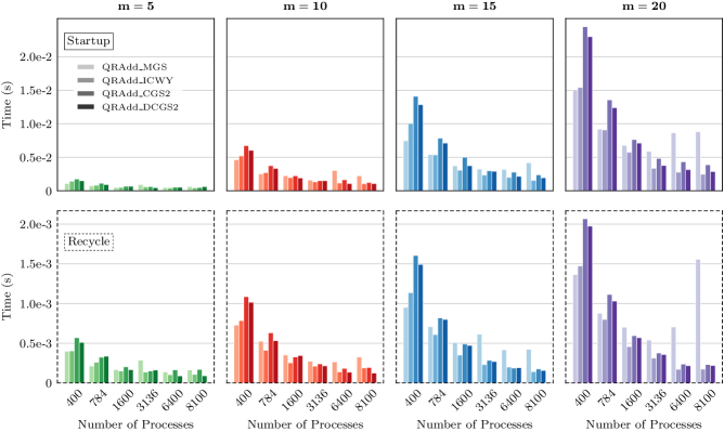
Figure 1: The cumulative time for the start-up iterations (top) and single recycle iteration (bottom) of the four different QRAdd kernels within AA for a vector of size $1\,048\,576$ on a varying number of Lassen CPU cores.

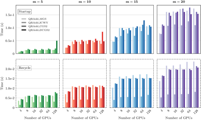
Figure 2: The cumulative time for the start-up iterations (top) and single recycle iteration (bottom) of the four different QRAdd kernels within AA for a local vector of size $1\,500\,000$ on a varying number of Lassen GPUs.

The top rows of Figure 1 (CPU) and Figure 2 (GPU) display the time required to fill the AA iteration space. As part of this operation, QRAdd_MGS requires $\sum_{k=1}^{m}k=\frac{m^{2}+m}{2}$ total synchronizations, while QRAdd_ICWY, QRAdd_CGS2, and QRAdd_DCGS require $2m-1$, $3m-2$, and $2m-1$, respectively.

Predicting performance based solely on the number of dot products performed, we expect that QRAdd_ICWY and QRAdd_DCGS2 will become faster than QRAdd_MGS after $m=3$ and QRAdd_CGS2 will outperform QRAdd_MGS after $m=6$, for processor counts where the synchronization imposed by dot products is the dominate cost. This is consistent with the CPU performance seen in Figure 1. The benefits of applying low synchronization QRAdd algorithms is not observed until the processor count reaches 1600 or higher when the global reduction costs lead to larger bottlenecks. As $m$ increases, the disparity between the time required for QRAdd_MGS and the low synchronization variants greatly increases.

Our observed GPU performance depends on the number of kernel calls for each QRAdd subroutine in addition to the number of global reductions. Compared to QRAdd_MGS, QRAdd_ICWY performs fewer CUDA kernels each iteration for $m>3$, while QRAdd_CGS2 and QRAdd_DCGS2 perform four additional CUDA kernel calls for $m>1$. Also, all three low synchronization variants perform sequential on-CPU updates to $R$, unlike QRAdd_MGS. Finally, in addition to the kernel launches and sequential updates, the low synchronization routines increase the amount of data being moved between the host and the GPU. Specifically, the fused dot products employed by these routines require that at most $m_{i}-1$ values be copied to and from the GPU multiple times per iteration while QRAdd_MGS copies only a single value per individual dot product.

All three low synchronization variants incur the cost of two kernel launches that require data transfers to and from the host process. However, in the case of QRAdd_ICWY, the lower computational requirements result in fewer overall CUDA kernel calls than for QRAdd_CGS2 and QRAdd_DCGS2. Specifically, 2 in Algorithm 5 and 4 in Algorithm 6 correspond to additional vector updates that are not required by QRAdd_ICWY; hence their performance times remain higher than QRAdd_ICWY independent of GPU count or $m$. There are minimal performance gains when using QRAdd_CGS2 or QRAdd_DCGS2 for filling the AA iteration space, as QRAdd_DCGS2 is only slightly faster than QRAdd_MGS when more than 8 GPUs are used and only for $m=15$ and larger.

4.2 Recycle Iterations

We next consider the cost of the QRAdd kernel once the AA iteration space is filled, namely the time required to orthogonalize a single vector against $m-1$ vectors. Assuming a large iteration count is required for convergence, this cost reflects the expected run-time of the QRAdd kernel for the majority of a given solve. We label these times as the “Recycle Iteration” time in Figures 1 and 2. The CPU and GPU timings presented are for the same global and local vector size as presented in Section 4.1, and the results are for a single iteration. Note that this time does not include the additional synchronization introduced by ICWY into QRDelete, first mentioned in Section 3.2 and discussed further in Section 5.

Once the AA iteration space is filled, the per iteration cost is greatly decreased by using one of the low synchronization orthogonalization algorithms when operating on CPUs (see the bottom row of Figure 1). While the “Startup Iterations” did not result in performance gains on CPUs until after 1600 processes, for $m>5$, we observe performance gains with QRAdd_ICWY with process counts as low as 784. QRAdd_MGS is still faster at smaller scales for all values of $m$ due to the reduced synchronization costs of performing an MPIAll_Reduce on a small, closed-set number of processes. The performance gains of the low synchronization algorithms at larger scales ranges from 2–8$\times$ speedup for $m=10$, $15$, and $20$ at $8100$ processes. With this drastic speedup for each iteration, we expect much larger performance gains for test problems that run to convergence.

Unlike the CPU performance for AA, QRAdd_ICWY demonstrates performance gains independent of the number of GPUs participating in the computation or the size of the AA iteration space, $m$. This is seen in the bottom row of Figure 2, which displays the performance for a single “Recycle Iteration” on multiple GPUs. While QRAdd_CGS2 and QRAdd_DCGS2 do not see the same performance improvements as QRAdd_ICWY, they do begin exhibiting faster performance than QRAdd_MGS beginning at 8 GPUs and for $m=10$ and larger, though gains are modest.

5 Numerical Experiments

In this section, we highlight the strong-scaling parallel efficiency of standard AA compared with AA with low synchronization orthogonalization for test problems run to convergence. The example problems provided are not exhaustive, but the selected tests do stress the performance of low synchronization AA. In addition, application specific tests are used to demonstrate the benefits of low synchronization AA for both distributed CPU and GPU computing environments. All experiments are performed on the LLNL Lassen supercomputer [12], with the same setup as described in Section 4. To account for machine variability, each run is executed 10 times and we report the minimum.

5.1 Anisotropic 2D Heat Equation + Nonlinear Term

This test problem highlights the performance of all AA variants for various $m$ and iterations to convergence. We consider a steady-state 2D heat equation with an additional nonlinear term $c(u)$,

$$u_{xx}+u_{yy}+c(u) =f\quad\text{in}\quad\mathcal{D}=[0,1]\times[0,1]$$

$$u =0\quad\text{on}\quad\partial\mathcal{D}.$$

The chosen analytical solution is

$$u_{\text{exact}}=u(x,y)=\sin^{2}(\pi x)\sin^{2}(\pi y),$$

hence, the static term $f$ is defined as follows

$$f(x,y)= 2\pi^{2}(\cos^{2}(\pi x)-\sin^{2}(\pi x))\sin^{2}(\pi y)$$

$$+2\pi^{2}(\cos^{2}(\pi y)-\sin^{2}(\pi y))\sin^{2}(\pi x)$$

$$+c(u_{\text{exact}}).$$

The spatial derivatives are computed using second-order centered differences, with the data distributed over $$1024$\times$1024$$ points on a uniform spatial grid, resulting in a system of equations of size $$1\,048\,576$\times$1\,048\,576$$. The Laplacian term is implemented as a matrix-vector product giving the the algebraic system as

$$A\boldsymbol{\mathrm{u}}+c(\boldsymbol{\mathrm{u}})=\boldsymbol{\mathrm{b}}.$$

where $\boldsymbol{\mathrm{u}}$ denotes the discrete vector of unknowns. Solving for $\boldsymbol{\mathrm{u}}$ results in the following FP formulation

$$\boldsymbol{\mathrm{u}}=G(\boldsymbol{\mathrm{u}})=A^{-1}(\boldsymbol{\mathrm{b}}-c(\boldsymbol{\mathrm{u}})).$$

We use the SUNDIALS PCG solver to solve the linear system with the hypre PFMG preconditioner performing two relaxation sweeps per iteration. Both the FP nonlinear solver and the PCG linear solver set a stopping criteria with a tolerance of $10^{-10}$. A zero vector is used as the starting guess in all cases.

5.1.1 Nonlinear Term 1

As a first example, consider the nonlinear reaction term

$$c(u)=u+ue^{u}+ue^{-u}+(u-e^{u})^{2}.$$

In this case, AA exhibits rapid convergence when $m=5$, requiring 11 iterations to converge for all variants. Figure 3 displays the overall time to convergence, split into $G(\boldsymbol{\mathrm{u}})$ evaluation time and time spent in AA. In general, the $G(\boldsymbol{\mathrm{u}})$ performance is volatile, most likely due to the sparse matrix operations required for the linear solve; thus we focus on the AA performance in the bottom of Figure 3.

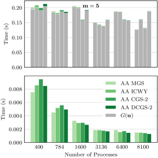
Figure 3: Time to convergence for Heat 2D + Nonlinear Term 1 (11 iterations for all cases), using FP + AA with $m=5$, including the function evaluation, $G(\boldsymbol{\mathrm{u}})$, (top) and only time in AA (bottom).

The time spent in AA meets expectations, based on the results in Section 4. For such a small $m$, we observe minimal performance improvements over AA with MGS, particularly at small process counts. However, the observed improvements begin around 1600 processes.

5.1.2 Nonlinear Term 2

As a second example, consider

$$c(u)=100\cdot(u-u^{2}).$$

With $m=10$, AA requires more time to converge than for the $c(u)$ in Section 5.1.1, better highlighting potential performance benefits of the low synchronization orthogonalization algorithms.

Figure 4 displays the overall timing results, with the number of iterations required to converge listed beneath each bar. In most cases, the number of iterations is between 27 and 42, depending on the orthogonalization method and processor count. The three exceptions are for AA with DCGS-2, which requires more iterations to converge, particularly for 1600–6400 processes. This is expected since our QRAdd_DCGS2 cannot lag the normalization and exhibits the same instability as Hernandez’s original algorithm.

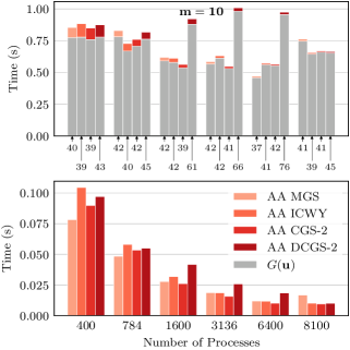
Figure 4: Time to convergence for Heat 2D + Nonlinear Term 2, using FP + AA with $m=10$, including the function evaluation, $G(\boldsymbol{\mathrm{u}})$, and the number of iterations to convergence (top) and only the time spent in AA (bottom).

In most cases, AA with DCGS-2 results in degraded performance in comparison to the other variants due to the high number of iterations required to converge. AA with CGS-2 performs best, starting at 1600 processes and continues to be the fastest through $8100$ processes. Although QRAdd_ICWY only requires two global synchronizations per iteration, there is an additional synchronization in QRDelete to update the matrix $T$, resulting in an implementation that is more comparable to AA with CGS-2 at higher process counts.

5.2 2D Bratu Problem

We next consider an example from [24] (and originating from [8]). The Bratu problem is a nonlinear PDE boundary value problem defined as:

$$u_{xx}+u_{yy}+\lambda e^{u} =0\quad\text{in}\quad\mathcal{D}=[0,1]\times[0,1]$$

$$u =0\quad\text{on}\quad\partial\mathcal{D}.$$

We again solve the problem with centered differencing, resulting in a system of the form

$$A\boldsymbol{\mathrm{u}}+\lambda e^{\boldsymbol{\mathrm{u}}}=0.$$

The associated FP function is then

$$G(\boldsymbol{\mathrm{u}})=A^{-1}\left(-\lambda e^{\boldsymbol{\mathrm{u}}}\right)=\boldsymbol{\mathrm{u}}.$$

We use a uniform grid of $1024\times 1024$ points, which results in a system of equations of size $$1\,048\,576$\times$1\,048\,576$$. We select $\lambda=6.7$ for testing, as it is close to the theoretical critical point, as discussed in [18], and is a difficult problem to solve. The SUNDIALS PCG solver is applied to perform the linear system solve with the hypre PFMG preconditioner performing two relaxation sweeps. Both the nonlinear and linear solver employed a tolerance of $10^{-10}$. A zero vector is set as the starting guess.

For this example problem, $m=30$, and the number of iterations required to converge for all variants of AA is less than 30; hence the timing results reflect the performance benefits of the QRAdd subroutines for the startup iterations. The strong-scaling timing and convergence results are presented in Figure 5. For this test case, we observe improvements with ICWY from the very beginning with 400 processes (although only slightly in this case). AA with ICWY continues to outperform up to 8100 processes. This is consistent with the results in Section 4.1 in which QRAdd_ICWY performed best for $m=20$ as it only requires two dot products per iteration, one fewer than QRAdd_CGS2 and has approximately the same amount of computation as QRAdd_DCGS2.

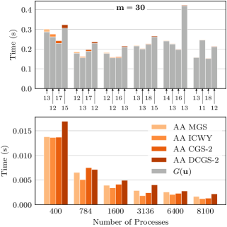
Figure 5: Time to convergence for 2D Bratu, using FP + AA with $m=30$, including the function evaluation, $G(\boldsymbol{\mathrm{u}})$, and the number of iterations to convergence (top) and only the time spent in AA (bottom).

5.3 Expectation-Maximization Algorithm for Mixture Densities

For this example, we consider a variation of the expectation-maximization test problem presented in [24]. Consider a mixture density of three univariate normal densities with a mixture density given by $p(x)=\sum_{i=1}^{3}\alpha_{i}p_{i}(x|\mu_{i},\sigma_{i})$, with

$$p_{i}(x|\mu_{i},\sigma_{i})=\frac{1}{\sqrt{2\pi}\sigma_{i}}e^{-(x-\mu_{i})^{2}/(2\sigma_{i}^{2})},\qquad 1\leq i\leq 3$$

Mixture proportions $\{\alpha_{i}\}_{i=1}^{3}$ are non-negative and sum to one. The mixture proportions and variances are assumed to be known and the means $\{\mu_{i}\}_{i=1}^{3}$ are estimated from a set of unlabeled samples $\{x_{k}\}_{k=1}^{N}$, or samples of unknown origin. Determining the unknown mean distribution parameters is given by the FP function

$$G(\mu_{i})=\mu_{i}=\frac{\sum_{k=1}^{N}x_{k}\frac{\alpha_{i}p_{i}(x_{k}|\mu_{i},\sigma_{i})}{p(x_{k})}}{\sum_{k=1}^{N}\frac{\alpha_{i}p_{i}(x_{k}|\mu_{i},\sigma_{i})}{p(x_{k})}},\qquad 1\leq i\leq 3$$

with current mean estimations $\{\mu_{i}\}_{i=1}^{3}$ being applied alongside the known mixture proportions and variances to determine the subsequent estimations until convergence. We keep the same mixture proportions and variances as the original test case, $(\alpha_{1},\alpha_{2},\alpha_{3})=(0.3,0.3,0.4)$ and $(\sigma_{1},\sigma_{2},\sigma_{3})=(1,1,1)$. We generated $100\,000$ samples for the mean distribution set $(\mu_{1}=0,\mu_{2}=0.5,\mu_{3}=1.0)$, corresponding to a poorly separated mixture, and used the same AA parameter of $m=3$ as Walker and Ni [24].

For our test case, we estimate a single set of mean distribution parameters redundantly for every entry in a global vector, where the vector takes the form

$$\boldsymbol{\mathrm{u}}=\begin{bmatrix}\{\mu_{i}\}_{i=1}^{3}&\cdots&\{\mu_{i}\}_{i=1}^{3}\end{bmatrix}.$$

We do this to simulate a function that requires no communication other than that imposed by AA. The resulting FP function to be solved is then given by

$$G(\boldsymbol{\mathrm{u}})=\begin{bmatrix}\{G(\mu_{i})\}_{i=1}^{3}&\cdots&\{G(\mu_{i})\}_{i=1}^{3}\end{bmatrix}.$$

Because $m$ is small for this test, we expect to see only modest improvements in performance of the low synchronization routines over MGS. For $m=3$, ICWY and DCGS-2 reduce the number of synchronizations per iteration by one over MGS, with ICWY gaining an additional synchronization after the space is filled.

The test is performed as a weak-scaling study with each GPU operating on a local vector size of $1\,500\,000$ values. Tests were run with a tolerance of $10^{-8}$, and each AA version requires 21 iterations to converge, independent of the orthogonalization subroutine used.

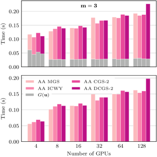
Figure 6: Time to convergence for Expectation-Maximization (21 iterations for all cases), using FP + AA with $m=3$ and a local vector size of $1\,500\,000$ for each GPU, including the function evaluation, $G(\boldsymbol{\mathrm{u}})$, (top) and only the time spent in AA (bottom).

The results of these tests are presented in Figure 6 and are consistent with the results of the weak-scaling study since no communication is required for $G(\boldsymbol{\mathrm{u}})$. The function evaluation performance remains the same, independent of GPU count or AA variant (differing only slightly for runs on a single node with 4 GPUs). In addition, the time spent in $G(\boldsymbol{\mathrm{u}})$ is lower for this example since $G(\boldsymbol{\mathrm{u}})$ performance depends on the number of samples in the mixture, while the performance of AA scales with the number of values in the global vector.

Results are consistent with observations in the GPU weak-scaling study in Section 4 where all of the QRAdd subroutines performed similar for $m=5$. Additionally, because $m$ is small, we do not incur a large overhead for data movement and multiple kernel launches in comparison to those observed with larger values of $m$, as presented in Section 4.2. Because the majority of the computation has moved to the GPU, we observe the expected cross-over point for ICWY with its performance being slightly faster than that of MGS for GPU counts of 16 and larger. There are no consistent improvements observed for CGS-2 or DCGS-2.

6 Conclusions

Anderson Acceleration (AA) is an efficient method for accelerating the convergence of fixed point solvers, but faces performance challenges in parallel distributed computing environments mainly due to the number of global synchronizations per iteration which is dependent upon the size of the AA iteration space. In this paper, we introduced low synchronization orthogonalization subroutines into AA which effectively reduce the number of global synchronizations to a constant number per iteration independent of the size of the AA iteration space. We presented a performance study that demonstrated the improved strong-scalability of AA with these low synchronization QRAdd subroutines when performed in a CPU-only parallel environment, as well as demonstrated performance and implementation concerns for these subroutines when operating in a multi-GPU computing environment. Furthermore, our numerical results display a realistic picture of the expected performance of AA in practice that matches the predictions of our performance analysis in Section 4 and suggests the use of ICWY for large values of $m$ when operating in a CPU-only parallel environment and as the default method for distributed GPU computing. Overall, this paper provides a comprehensive study of low synchronization orthogonalization routines within AA and their parallel performance benefits.

The software used to generate the results in this paper will be available in a future release of SUNDIALS.

References

- [1] N. N. Abdelmalek, Round off error analysis for Gram-Schmidt method and solution of linear least squares problems, BIT Numerical Mathematics, 11 (1971), pp. 345–367.
- [2] D. G. Anderson, Iterative procedures for nonlinear integral equations, J. Assoc. Comput. Mach., 12 (1965), pp. 547–560, https://doi.org/10.1145/321296.321305.
- [3] C. J. Balos, D. J. Gardner, C. S. Woodward, and D. R. Reynolds, Enabling GPU accelerated computing in the sundials time integration library, Parallel Computing, (2021), p. 102836, https://doi.org/10.1016/j.parco.2021.102836.
- [4] D. Bielich, J. Langou, S. Thomas, K. Świrydowicz, I. Yamazaki, and E. Boman, Low-synch Gram-Schmidt with delayed reorthogonalization for Krylov solvers, Parallel Computing, (2021).
- [5] Å. Björck, Solving linear least squares problems by Gram-Schmidt orthogonalization, BIT Numerical Mathematics, 7 (1967), pp. 1–21.
- [6] J. W. Daniel, W. B. Gragg, L. Kaufman, and G. W. Stewart, Reorthogonalization and stable algorithms for updating the Gram-Schmidt QR factorization, Mathematics of Computation, 30 (1976), pp. 772–795.
- [7] H. Fang and Y. Saad, Two classes of multisecant methods for nonlinear acceleration, Numer. Linear Algebra Appl., 16 (2009), pp. 197–221.
- [8] D. A. Frank-Kamenetskii, Diffusion and Heat Exchange in Chemical Kinetics, Princeton University Press, 2016, https://doi.org/10.1515/9781400877195.
- [9] V. Frayssé, L. Giraud, and H. Kharraz-Aroussi, On the influence of the orthogonalization scheme on the parallel performance of GMRES, in European Conference on Parallel Processing, Springer, 1998, pp. 751–762.
- [10] L. Giraud, J. Langou, M. Rozložník, and J. van den Eshof, Rounding error analysis of the classical Gram-Schmidt orthogonalization process, Numer. Math., 101 (2005), p. 87–100, https://doi.org/10.1007/s00211-005-0615-4.
- [11] L. Giraud, J. Langou, and M. Rozloznik, The loss of orthogonality in the Gram-Schmidt orthogonalization process, Computers & Mathematics with Applications, 50 (2005), pp. 1069–1075, https://doi.org/10.1016/j.camwa.2005.08.009. Numerical Methods and Computational Mechanics.
- [12] W. A. Hanson, The CORAL supercomputer systems, IBM Journal of Research and Development, 64 (2020), pp. 1:1–1:10.
- [13] V. Hernández, J. E. Román, and A. Tomás, A parallel variant of the Gram-Schmidt process with reorthogonalization, in PARCO, 2005, pp. 221–228.
- [14] A. C. Hindmarsh, R. Serban, C. J. Balos, D. J. Gardner, D. R. Reynolds, and C. S. Woodward, User documentation for KINSOL v5. 7.0 (SUNDIALS v5. 7.0), 2021, https://computing.llnl.gov/projects/sundials/kinsol.
- [15] W. Hoffmann, Iterative algorithms for Gram-Schmidt orthogonalization, Computing, 41 (1989), pp. 335–348.
- [16] C. T. Kelley, Numerical methods for nonlinear equations, Acta Numerica, 27 (2018), pp. 207–287.
- [17] J. Loffeld and C. S. Woodward, Considerations on the implementation and use of anderson acceleration on distributed memory and GPU-based parallel computers, in Advances in the Mathematical Sciences, Springer, 2016, pp. 417–436.
- [18] A. Mohsen, A simple solution of the Bratu problem, Computers & Mathematics with Applications, 67 (2014), pp. 26–33, https://doi.org/10.1016/j.camwa.2013.10.003.
- [19] C. C. Paige, The effects of loss of orthogonality on large scale numerical computations, in Proceedings of the International Conference on Computational Science and Its Applications, Springer-Verlag, 05 2018, pp. 429–439.
- [20] B. N. Parlett, The symmetric eigenvalue problem, SIAM, 1998.
- [21] A. Ruhe, Numerical aspects of Gram-Schmidt orthogonalization of vectors, Linear algebra and its applications, 52 (1983), pp. 591–601.
- [22] Y. Saad and M. H. Schultz, GMRES: A generalized minimal residual algorithm for solving nonsymmetric linear systems, SIAM Journal on scientific and statistical computing, 7 (1986), pp. 856–869.
- [23] K. Świrydowicz, J. Langou, S. Ananthan, U. Yang, and S. Thomas, Low synchronization Gram–Schmidt and generalized minimal residual algorithms, Numerical Linear Algebra with Applications, 28 (2021), p. e2343, https://doi.org/10.1002/nla.2343.
- [24] H. F. Walker and P. Ni, Anderson acceleration for fixed-point iterations, SIAM Journal on Numerical Analysis, 49 (2011), pp. 1715–1735, https://doi.org/10.1137/10078356X.
- [25] I. Yamazaki, S. Thomas, M. Hoemmen, E. G. Boman, K. Świrydowicz, and J. J. Elliott, Low-synchronization orthogonalization schemes for s-step and pipelined Krylov solvers in trilinos, in Proceedings of the 2020 SIAM Conference on Parallel Processing for Scientific Computing, SIAM, 2020, pp. 118–128.