System Norm Regularization Methods for Koopman Operator Approximation

Abstract

Approximating the Koopman operator from data is numerically challenging when many lifting functions are considered. Even low-dimensional systems can yield unstable or ill-conditioned results in a high-dimensional lifted space. In this paper, Extended Dynamic Mode Decomposition (DMD) and DMD with control, two methods for approximating the Koopman operator, are reformulated as convex optimization problems with linear matrix inequality constraints. Asymptotic stability constraints and system norm regularizers are then incorporated as methods to improve the numerical conditioning of the Koopman operator. Specifically, the $\mathcal{H}_{\infty}$ norm is used to penalize the input-output gain of the Koopman system. Weighting functions are then applied to penalize the system gain at specific frequencies. These constraints and regularizers introduce bilinear matrix inequality constraints to the regression problem, which are handled by solving a sequence of convex optimization problems. Experimental results using data from an aircraft fatigue structural test rig and a soft robot arm highlight the advantages of the proposed regression methods.

1 Introduction

Koopman operator theory [1, 2, 3, 4] allows a nonlinear system to be exactly represented as a linear system in terms of an infinite set of lifting functions. The Koopman operator advances each of these lifting function to the next timestep. Thanks to recent theoretical developments [2, 3, 4] and the widespread availability of computational resources, there has been a recent resurgence of interest in using data-driven methods to approximate the Koopman operator. The Koopman operator defines a linear state-space system in the chosen lifted space, making it convenient for control system design. Koopman models have been paired with a wide variety of existing linear optimal control techniques [5, 6, 7, 8, 9, 10] with great success.

Figure 1: Overview of the data-driven Koopman workflow, including the role of the proposed regression methods. (a) First, data is collected from the system to be identified. (b) Next, a set of lifting functions is chosen. (c) The lifting functions are then applied to the data and snapshot matrices are formed. (d) Finally, one of several regression methods is used to approximate the Koopman matrix. The proposed regression methods seek to address the numerical problems often present in this step by viewing it as an optimization over discrete-time linear systems.

To use the Koopman representation in practical applications, a finite-dimensional approximation of the infinite-dimensional Koopman operator must be found. First, a finite set of lifting functions is selected. These functions are often hand-picked based on known dynamics [7, 8], or are combinations of sinusoids, polynomials, and other basis functions [9, 11]. Time delay embeddings are also popular [5, 9]. However, there is no universally agreed-upon method for selecting lifting functions. Given a set of lifting functions, linear regression is used to find the matrix approximation of the Koopman operator, also called a Koopman matrix [12, 6].

Unfortunately, the regression problem associated with finding an approximate Koopman operator is numerically challenging, as complex lifting function choices can yield unstable or ill-conditioned Koopman models for stable systems [13]. Regularization techniques play a crucial role in obtaining usable Koopman models for prediction and control applications. Standard regularization techniques like Tikhonov regularization [14] or the lasso [15] are often used to promote well-conditioned Koopman matrices. These regularization techniques penalize different matrix norms of the Koopman matrix, without considering the fact that the Koopman matrix defines a discrete-time linear system with input, state, and output. While these methods may indirectly promote asymptotic stability in this Koopman system, their success is highly dependent on the regularization coefficient used. Furthermore, they do not consider the input-output gain of the Koopman system. This paper takes a systems view of the Koopman matrix regression problem, proposing regression methods that constrain the asymptotic stability of the Koopman system and regularize the regression problem by penalizing its input-output gain, as represented by its $\mathcal{H}_{\infty}$ norm. To accomplish this, the Extended Dynamic Mode Decomposition (EDMD) [16] and Dynamic Mode Decomposition with control (DMDc) [17] methods are reformulated as convex optimization problems with linear matrix inequality (LMI) constraints. Regularizers and additional constraints are incorporated in a modular fashion as either LMI constraints, or bilinear matrix inequality (BMI) constraints. The data-driven Koopman workflow and the proposed regression methods are summarized in fig. 1.

1.1 Related work

Convex optimization and LMIs have previously been used to synthesize controllers for Koopman models [10], but they have not yet been leveraged to regularize the Koopman matrix regression problem. A related optimization problem is posed in [18], where both the Koopman matrix and lifting functions are treated as unknowns. While this problem is NP-hard, a convex relaxation allows both to be found by solving two semidefinite programs. The $\mathcal{H}_{\infty}$ norm of the Koopman operator has previously been considered in [19], however it is in the form of a hard constraint on the system’s dissipativity, rather than as a regularizer in the cost function.

In [20], the problem of learning Lyapunov stable and asymptotically stable linear systems is explored in the context of subspace identification, where Lyapunov inequalities are used to enforce the corresponding stability conditions. The related problem of learning positive real and strictly positive real systems using constrained subspace identification is discussed in [21]. A convex relaxation of the Lyapunov inequality is considered in [22], where linear constraints are added incrementally to enforce the Lyapunov stability of a system. In [13], a gradient-descent method called SOC [23] is applied to find locally optimal Lyapunov stable or asymptotically stable Koopman matrices. The method relies on a parameterization of the Koopman matrix that guarantees Lyapunov stability or asymptotic stability [24]. While addressing the asymptotic stability problem, this formulation lacks the modularity of the proposed approach.

1.2 Contribution

The core contributions of this paper are solving the EDMD and DMDc problems with asymptotic stability constraints and with system norm regularizers. Of particular focus is the use of the $\mathcal{H}_{\infty}$ norm as a regularizer, which penalizes the worst-case gain of the Koopman system over all frequencies. The BMI formulation of the EDMD problem with asymptotic stability constraints and $\mathcal{H}_{\infty}$ norm regularization were previously explored by the authors in [25]. LMI formulations for Tikhonov regularization, matrix two-norm regularization, and nuclear norm regularization were also presented in [25]. This paper expands on [25] to include an LMI formulation of the DMDc problem, and discusses the corresponding asymptotic stability constraint and $\mathcal{H}_{\infty}$ norm regularizer. As with EDMD, these modifications add BMI constraints to the DMDc problem. Furthermore, weighted $\mathcal{H}_{\infty}$ norm regularization is explored, which allows the Koopman system’s gain to be penalized in a specific frequency band, where experimental measurements may be less reliable, or where system dynamics may be irrelevant. Finally, the proposed regression methods are evaluated using two experimental datasets, one from a fatigue structural testing platform, and the other from a soft robot arm. The significance of this work is the use of a system norm to regularize the Koopman regression problem, which is viewed as a regression problem over discrete-time linear systems, resulting in a numerically better conditioned data-driven model.

2 Background

2.1 Koopman operator theory

Consider the discrete-time nonlinear process

$$\mbf{x}_{k+1}=\mbf{f}(\mbf{x}_{k}),$$ (1)

where ${\mbf{x}_{k}\in\mathcal{M}}$ evolves on a manifold ${\mathcal{M}\subseteq\mathbb{R}^{m\times 1}}$. Let ${\psi:\mathcal{M}\to\mathbb{R}}$ be a lifting function. Any scalar function of the state $\mbf{x}_{k}$ qualifies as a lifting function. The lifting functions therefore form an infinite-dimensional Hilbert space $\mathcal{H}$. The Koopman operator ${\mathcal{U}:\mathcal{H}\to\mathcal{H}}$ is a linear operator that advances all scalar-valued lifting functions ${\psi\in\mathcal{H}}$ in time by one timestep. That is [12, §3.2],

$$(\mathcal{U}\psi)(\cdot)=(\psi\circ\mbf{f})(\cdot).$$ (2)

Using eq. 2, the dynamics of eq. 1 can be rewritten linearly in terms of $\psi$ as

$$\psi(\mbf{x}_{k+1})=(\mathcal{U}\psi)(\mbf{x}_{k}).$$ (3)

In finite dimensions, eq. 3 is approximated by

$$\bm{\psi}(\mbf{x}_{k+1})=\mbf{U}\bm{\psi}(\mbf{x}_{k})+\mbf{r}_{k},$$ (4)

where ${\bm{\psi}:\mathcal{M}\to\mathbb{R}^{p\times 1}}$, ${\mbf{U}\in\mathbb{R}^{p\times p}}$, and $\mbf{r}_{k}$ is the residual error. Each element of the vector-valued lifting function $\bm{\psi}$ is a lifting function in $\mathcal{H}$. The Koopman matrix $\mbf{U}$ is a matrix approximation of the Koopman operator.

2.2 Koopman operator theory with inputs

If a discrete-time nonlinear process with exogenous inputs is considered, the definitions of the lifting functions and Koopman operator must be modified. Consider

$$\mbf{x}_{k+1}=\mbf{f}(\mbf{x}_{k},\mbf{u}_{k}),$$ (5)

where ${\mbf{x}_{k}\in\mathcal{M}\subseteq\mathbb{R}^{m\times 1}}$ and ${\mbf{u}_{k}\in\mathcal{N}\subseteq\mathbb{R}^{n\times 1}}$. In this case, the lifting functions become ${\psi:\mathcal{M}\times\mathcal{N}\to\mathbb{R}}$ and the Koopman operator ${\mathcal{U}:\mathcal{H}\to\mathcal{H}}$ is instead defined so that

$$(\mathcal{U}\psi)(\mbf{x}_{k},\mbf{u}_{k})=\psi(\mbf{f}(\mbf{x}_{k},\mbf{u}_{k}),\star),$$ (6)

where ${\star=\mbf{u}_{k}}$ if the input has state-dependent dynamics, or ${\star=\mbf{0}}$ if the input has no dynamics [12, §6.5]. If the input is computed by a controller, it is often considered to have state-dependent dynamics. Let the vector-valued lifting function ${\bm{\psi}:\mathcal{M}\times\mathcal{N}\to\mathbb{R}^{p\times 1}}$ be partitioned as

$$\bm{\psi}(\mbf{x}_{k},\mbf{u}_{k})=\begin{bmatrix}\bm{\vartheta}(\mbf{x}_{k})\\ \bm{\upsilon}(\mbf{x}_{k},\mbf{u}_{k})\end{bmatrix},$$ (7)

where ${\bm{\vartheta}:\mathcal{M}\to\mathbb{R}^{p_{\vartheta}\times 1}}$, ${\bm{\upsilon}:\mathcal{M}\times\mathcal{N}\to\mathbb{R}^{p_{\upsilon}\times 1}}$, and ${p_{\vartheta}+p_{\upsilon}=p}$. When the input is exogenous, eq. 6 has the form [12, §6.5.1]

$$\bm{\vartheta}(\mbf{x}_{k+1})\\ =\mbf{U}\bm{\psi}(\mbf{x}_{k},\mbf{u}_{k})+\mbf{r}_{k},$$ (8)

where ${\mbf{U}=\begin{bmatrix}\mbf{A}&\mbf{B}\end{bmatrix}}$. Expanding eq. 8 yields the familiar linear state-space form,

$$\bm{\vartheta}(\mbf{x}_{k+1})=\mbf{A}\bm{\vartheta}(\mbf{x}_{k})+\mbf{B}\bm{\upsilon}(\mbf{x}_{k},\mbf{u}_{k})+\mbf{r}_{k}.$$ (9)

When identifying a Koopman model for control, the input is often left unlifted, that is, ${\bm{\upsilon}(\mbf{x}_{k},\mbf{u}_{k})=\mbf{u}_{k}}$ [5]. However, recent work demonstrates that this choice of lifting functions is insufficient for describing control affine systems, which are ubiquitous in real-world applications [26]. An alternative choice of input-dependent lifting functions proposed in [26] is

$$\bm{\upsilon}(\mbf{x}_{k},\mbf{u}_{k})=\begin{bmatrix}\mbf{u}_{k}\otimes\bm{\vartheta}(\mbf{x}_{k})\\ \mbf{u}_{k}\end{bmatrix},$$ (10)

where $\otimes$ denotes the Kronecker product. These bilinear input-dependent lifting functions are capable of representing all control affine systems, and therefore present an interesting alternative to leaving the input unlifted [26].

2.3 Approximating the Koopman operator from data

To approximate the Koopman matrix from a dataset ${\mathcal{D}={\{\mbf{x}_{k},\mbf{u}_{k}\}}_{k=0}^{q}}$, consider the lifted snapshot matrices

$$\bm{\Psi} =\begin{bmatrix}\bm{\psi}_{0}&\bm{\psi}_{1}&\cdots&\bm{\psi}_{q-1}\end{bmatrix}\in\mathbb{R}^{p\times q},$$ (11)

$$\bm{\Theta}_{+} =\begin{bmatrix}\bm{\vartheta}_{1}&\bm{\vartheta}_{2}&\cdots&\bm{\vartheta}_{q}\end{bmatrix}\in\mathbb{R}^{p_{\vartheta}\times q},$$ (12)

where ${\bm{\psi}_{k}=\bm{\psi}(\mbf{x}_{k},\mbf{u}_{k})}$ and ${\bm{\vartheta}_{k}=\bm{\vartheta}(\mbf{x}_{k})}$. The Koopman matrix that minimizes

$$J(\mbf{U})=\|\bm{\Theta}_{+}-\mbf{U}\bm{\Psi}\|_{\mathsf{F}}^{2}$$ (13)

is [12, §1.2.1]

$$\mbf{U}=\bm{\Theta}_{+}\bm{\Psi}^{\dagger},$$ (14)

where ${(\cdot)}^{\dagger}$ denotes the Moore-Penrose pseudoinverse.

3 Reformulating the Koopman Operator Regression Problem

3.1 Extended DMD

The direct least-squares method of approximating the Koopman operator in eq. 14 is fraught with numerical and performance issues. Namely, computing the pseudoinverse of $\bm{\Psi}$ is costly when the dataset contains many snapshots. Extended Dynamic Mode Decomposition (EDMD) [16] reduces the dimension of the pseudoinverse required to compute eq. 14 when the number of snapshots is much larger than the dimension of the lifted state (i.e. , ${p\ll q}$) [12, §10.3].

Extended DMD consists of computing eq. 14 using

$$\mbf{U}=\bm{\Theta}_{+}\left(\bm{\Psi}^{\mathsf{T}}\bm{\Psi}^{{\mathsf{T}}^{\dagger}}\right)\bm{\Psi}^{\dagger}=\left(\bm{\Theta}_{+}\bm{\Psi}^{\mathsf{T}}\right){\left(\bm{\Psi}\bm{\Psi}^{\mathsf{T}}\right)}^{\dagger}=\mbf{G}\mbf{H}^{\dagger},$$ (15)

where

$$\mbf{G}=\frac{1}{q}\bm{\Theta}_{+}\bm{\Psi}^{\mathsf{T}}\in\mathbb{R}^{p_{\vartheta}\times p},\quad\mbf{H}=\frac{1}{q}\bm{\Psi}\bm{\Psi}^{\mathsf{T}}\in\mathbb{R}^{p\times p}.$$ (16)

Now, only a ${p\times p}$ pseudoinverse is required, rather than a ${p\times q}$ pseudoinverse. To improve numerical conditioning, $\mbf{G}$ and $\mbf{H}$ are often scaled by the number of snapshots $q$, as in eq. 16. Note that ${\mbf{H}=\mbf{H}^{\mathsf{T}}>0}$ if the columns of $\bm{\Psi}$ are linearly independent.

3.2 LMI reformulation of EDMD

To incorporate regularizers and constraints in a modular fashion, the Koopman operator regression problem is reformulated as a convex optimization problem with LMI constraints. Recall that the Koopman matrix $\mbf{U}$ minimizes eq. 13. It therefore also minimizes

$$J(\mbf{U}) =\frac{1}{q}\|\bm{\Theta}_{+}-\mbf{U}\bm{\Psi}\|_{\mathsf{F}}^{2}=\frac{1}{q}{\mathrm{tr}}{\left(\left(\bm{\Theta}_{+}-\mbf{U}\bm{\Psi}\right){\left(\bm{\Theta}_{+}-\mbf{U}\bm{\Psi}\right)}^{\mathsf{T}}\right)}$$ (17)

$$={\mathrm{tr}}{\left(\frac{1}{q}\bm{\Theta}_{+}\bm{\Theta}_{+}^{\mathsf{T}}-{\mathrm{He}\!\left\{\mbf{U}\mbf{G}^{\mathsf{T}}\right\}}+\mbf{U}\mbf{H}\mbf{U}^{\mathsf{T}}\right)}$$ (18)

$$=c-2{\mathrm{tr}}{\left(\mbf{U}\mbf{G}^{\mathsf{T}}\right)}+{\mathrm{tr}}{\left(\mbf{U}\mbf{H}\mbf{U}^{\mathsf{T}}\right)},$$ (19)

where $c=\frac{1}{q}\bm{\Theta}_{+}\bm{\Theta}_{+}^{\mathsf{T}}$ is a scalar constant, $\mbf{G}$ and $\mbf{H}$ are defined in eq. 16, and ${{\mathrm{He}\!\left\{\cdot\right\}}={(\cdot)}+{(\cdot)}^{\mathsf{T}}}$. The minimization of eq. 19 is equivalent to the minimization of

$$J(\mbf{U},\mbf{\nu},\mbf{W})=c-2{\mathrm{tr}}{\left(\mbf{U}\mbf{G}^{\mathsf{T}}\right)}+\nu$$ (20)

subject to

$${\mathrm{tr}}{(\mbf{W})}<\nu,\quad\mbf{W}>0,\quad\mbf{U}\mbf{H}\mbf{U}^{\mathsf{T}}<\mbf{W},$$ (21)

where $\nu$ and $\mbf{W}$ are slack variables that allow the cost function to be rewritten using LMIs [27, §2.15.1]. To rewrite the quadratic term in eq. 21 as an LMI, consider the matrix decomposition ${\mbf{H}=\mbf{L}\mbf{L}^{\mathsf{T}}}$. The matrix $\mbf{L}$ can be found using a Cholesky factorization or eigendecomposition of $\mbf{H}$, or a singular value decomposition of $\bm{\Psi}$. Assuming the decomposition has been performed, the quadratic term in the optimization problem becomes

$$\mbf{W}-\mbf{U}\mbf{H}\mbf{U}^{\mathsf{T}}=\mbf{W}-\mbf{U}\mbf{L}\mbf{L}^{\mathsf{T}}\mbf{U}^{\mathsf{T}}=\mbf{W}-\left(\mbf{U}\mbf{L}\right)\mbf{1}{\left(\mbf{U}\mbf{L}\right)}^{\mathsf{T}},$$ (22)

where $\mbf{1}$ is the identity matrix. Applying the Schur complement [27, §2.3.1] to eq. 22 yields

$$\begin{bmatrix}\mbf{W}&\mbf{U}\mbf{L}\\ \mbf{L}^{\mathsf{T}}\mbf{U}^{\mathsf{T}}&\mbf{1}\end{bmatrix}>0.$$ (23)

The LMI form of the optimization problem is therefore

$$\min\; J(\mbf{U},\mbf{\nu},\mbf{W})=c-2{\mathrm{tr}}{\left(\mbf{U}\mbf{G}^{\mathsf{T}}\right)}+\nu$$ (24)

$$\mathrm{s.t.}\; {\mathrm{tr}}{(\mbf{W})}<\nu,\quad\mbf{W}>0,\quad\begin{bmatrix}\mbf{W}&\mbf{U}\mbf{L}\\ \mbf{L}^{\mathsf{T}}\mbf{U}^{\mathsf{T}}&\mbf{1}\end{bmatrix}>0,$$ (25)

where ${\mbf{H}=\mbf{L}\mbf{L}^{\mathsf{T}}}$.

As previously mentioned, the decomposition ${\mbf{H}=\mbf{L}\mbf{L}^{\mathsf{T}}}$ can be realized via a Cholesky factorization, eigendecomposition, or singular value decomposition. Using a Cholesky factorization directly gives $\mbf{L}$. When using an eigendecomposition, ${\mbf{H}=\mbf{V}\bm{\Lambda}\mbf{V}^{\mathsf{T}}}$, it follows that $\mbf{L}=\mbf{V}\sqrt{\bm{\Lambda}}$. Alternatively, using a singular value decomposition, $\bm{\Psi}=\mbf{Q}\bm{\Sigma}\mbf{Z}^{\mathsf{T}}$, and substituting it into the definition of $\mbf{H}$ in eq. 16 yields ${\mbf{H}=\frac{1}{q}\mbf{Q}\bm{\Sigma}^{2}\mbf{Q}^{\mathsf{T}}}$. It follows that $\mbf{L}=\frac{1}{\sqrt{q}}\mbf{Q}\bm{\Sigma}.$ A singular value decomposition is used to compute $\mbf{L}$ in the experiments presented in this paper.

4 Asymptotic Stability Constraint

Since many systems of interest have asymptotically stable dynamics, it is desirable to identify Koopman systems that share this property. In [13], it is proven that an asymptotically stable nonlinear system can only be represented accurately by an asymptotically stable Koopman system, thus highlighting the importance of enforcing the asymptotic stability property during the regression process.

However, in practice, it is possible to identify an unstable Koopman system from measurements of an asymptotically stable system [13]. Even if the identified Koopman system is asymptotically stable in theory, the eigenvalues of its $\mbf{A}$ matrix may be so close to the unit circle that it is effectively unstable in practice. One solution, presented in this section, is to constrain the largest eigenvalue of $\mbf{A}$ to be strictly less than one in magnitude, within a desired tolerance.

4.1 Constraint formulation

To ensure that the system defined by the Koopman matrix ${\mbf{U}=\begin{bmatrix}\mbf{A}&\mbf{B}\end{bmatrix}}$ is asymptotically stable, the eigenvalues of $\mbf{A}$ must be constrained to have magnitude strictly less than one. A modified Lyapunov constraint [28, §1.4.4]

$$\mbf{P} >0,$$ (26)

$$\mbf{A}^{\mathsf{T}}\mbf{P}\mbf{A}-\bar{\rho}^{2}\mbf{P} <0,$$ (27)

can be added to ensure that the magnitude of the largest eigenvalue of $\mbf{A}$ is no larger than ${0<\bar{\rho}<1}$. Applying the Schur complement to eq. 27 yields

$$\mbf{A}^{\mathsf{T}}\mbf{P}\mbf{A}-\bar{\rho}^{2}\mbf{P}<0 \iff\left(\mbf{A}^{\mathsf{T}}\mbf{P}\right)\mbf{P}^{-1}{\left(\mbf{A}^{\mathsf{T}}\mbf{P}\right)}^{\mathsf{T}}-\bar{\rho}^{2}\mbf{P}<0$$ (28)

$$\iff-\bar{\rho}\mbf{P}-\left(-\mbf{A}^{\mathsf{T}}\mbf{P}\right){\left(-\bar{\rho}\mbf{P}\right)}^{-1}{\left(-\mbf{A}^{\mathsf{T}}\mbf{P}\right)}^{\mathsf{T}}<0$$ (29)

$$\iff\begin{bmatrix}-\bar{\rho}\,\mbf{P}&-\mbf{A}^{\mathsf{T}}\mbf{P}\\ -\mbf{P}^{\mathsf{T}}\mbf{A}&-\bar{\rho}\,\mbf{P}\end{bmatrix}<0,\ -\bar{\rho}\,\mbf{P}<0$$ (30)

$$\iff\begin{bmatrix}\bar{\rho}\,\mbf{P}&\mbf{A}^{\mathsf{T}}\mbf{P}\\ \mbf{P}^{\mathsf{T}}\mbf{A}&\bar{\rho}\,\mbf{P}\end{bmatrix}>0,\ \mbf{P}>0.$$ (31)

The full optimization problem with asymptotic stability constraint is therefore

$$\min\; J(\mbf{U},\mbf{\nu},\mbf{W},\mbf{P};\bar{\rho})=c-2{\mathrm{tr}}{\left(\mbf{U}\mbf{G}^{\mathsf{T}}\right)}+\nu$$ (32)

$$\mathrm{s.t.}\; {\mathrm{tr}}{(\mbf{W})}<\nu,\quad\mbf{W}>0,\quad\begin{bmatrix}\mbf{W}&\mbf{U}\mbf{L}\\ \mbf{L}^{\mathsf{T}}\mbf{U}^{\mathsf{T}}&\mbf{1}\end{bmatrix}>0,\quad\mbf{P}>0,\quad\begin{bmatrix}\bar{\rho}\,\mbf{P}&\mbf{A}^{\mathsf{T}}\mbf{P}\\ \mbf{P}^{\mathsf{T}}\mbf{A}&\bar{\rho}\,\mbf{P}\end{bmatrix}>0,$$ (33)

where ${\mbf{H}=\mbf{L}\mbf{L}^{\mathsf{T}}}$ and ${\mbf{U}=\begin{bmatrix}\mbf{A}&\mbf{B}\end{bmatrix}}$.

Since both $\mbf{A}$ and $\mbf{P}$ are unknown, eq. 31 includes a BMI constraint. The optimization problem is therefore nonconvex and NP-hard. One method to find a locally optimal solution is outlined in [29]. First, assume $\mbf{P}$ is constant with an initial guess of $\mbf{P}=\mbf{1}$ and solve eqs. 32 to 33 as an LMI problem. Then, hold the remaining variables constant using the solution from that optimization, and solve a feasibility problem for $\mbf{P}$. Repeat this process until the cost function stops changing significantly. Although this approach is rather simple, it does result in an asymptotically stable Koopman system with reasonable prediction error.

4.2 Experimental results

The effectiveness of the proposed asymptotic stability constraint is demonstrated using experimental data collected from the Fatigue Structural Testing Equipment Research (FASTER) platform at the National Research Council of Canada (NRC) [30], which is used for aircraft fatigue testing research.

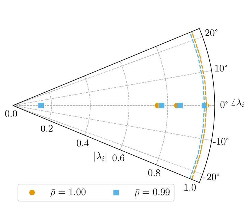
(a)

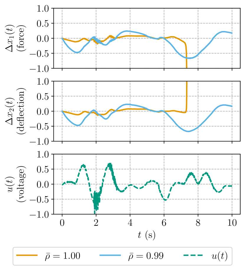
(b)

Figure 2: (2(a)) Eigenvalues and spectral radius constraints of Koopman $\mbf{A}$ matrices approximated from the FASTER dataset. The eigenvalues of $\mbf{A}$ satisfy their respective spectral radius constraints. Additionally, lowering the spectral radius constraint from ${\bar{\rho}=1.00}$ to ${\bar{\rho}=0.99}$ does not significantly alter the eigenvalues. (2(b)) Multi-step prediction error of Koopman systems approximated from the FASTER dataset. All units are normalized. States are recovered and re-lifted between prediction timesteps. Although both systems are asymptotically stable, only the system with ${\bar{\rho}=0.99}$ is usable in practice, as the other system’s response diverges due to the accumulation of numerical error.

In the fatigue structural testing dataset used in this paper, the structure under test is an aluminum-composite beam. During a test, the FASTER platform applies a force to this beam using a hydraulic actuator, which is controlled by a voltage. This input, the applied force, and the structure’s deflection are recorded at $128\text{\,}\mathrm{Hz}$. The actuator voltage is determined by a linear controller designed to track a reference force profile. In this case, the dynamics of the controller are neglected and the actuator voltage is considered to be exogenous. All states and inputs in the FASTER dataset are normalized. A photograph of this experimental setup can be found in [30].

The Koopman lifting functions chosen for the FASTER platform are first- and second-order monomials. The full lifting procedure consists of several steps to improve numerical conditioning. First, all states and inputs are normalized so that they do not grow when passed through the monomial lifting functions. Then, all first- and second-order monomials of the state and input are computed. Finally, the lifted states are standardized to ensure that they are evenly weighted in the regression. To standardize the lifted states, their means are subtracted and they are rescaled to have unit variance [31, §4.6.6]. When using the identified Koopman matrices for prediction, the state and input are lifted, then multiplied by the Koopman matrix. The state is then recovered and re-lifted with the input for the next timestep. Using this prediction method leads to the local error definition presented in [13], which is used throughout this paper.

Given that the true FASTER system is asymptotically stable, it is crucial to ensure that the identified Koopman system shares this property. To demonstrate the impact of the asymptotic stability constraint, Koopman matrices with maximum spectral radii of ${\bar{\rho}=1.00}$ and ${\bar{\rho}=0.99}$ are computed and compared to an unconstrained Koopman matrix computed with standard EDMD. Figure 2(a) shows the eigenvalues of the two constrained Koopman $\mbf{A}$ matrices. In both cases, the eigenvalues indicate that the systems obey their respective maximum spectral radii. However, the multi-step prediction errors of the two Koopman systems in fig. 2(b) show that only the system with the spectral radius constraint of ${\bar{\rho}=0.99}$ is usable in practice. The other system produces prediction errors that diverge to infinity due to the accumulation of numerical error. The Koopman matrix without asymptotic stability constraint behaves identically to the matrix with maximum spectral radius ${\bar{\rho}=1.00}$, and is therefore not shown fig. 2. By introducing a small amount of conservatism in the spectral radius constraint, the identified Koopman system is rendered asymptotically stable in the face of accumulated numerical error.

5 System Norm Regularization

While constraining the asymptotic stability of the identified Koopman system helps ensure that the system’s predictions are usable, it does not consider the input-output properties of the system. A system norm like the $\mathcal{H}_{2}$ norm or the $\mathcal{H}_{\infty}$ norm can be used to regularize the system’s gain, while also ensuring asymptotic stability for any regularization coefficient. Specifically, the existence of a finite $\mathcal{H}_{2}$ or $\mathcal{H}_{\infty}$ norm guarantees the asymptotic stability of the resulting linear time-invariant (LTI) system [32]. Regularizing using the $\mathcal{H}_{2}$ norm can be thought of as penalizing the average system gain over all frequencies, while using the $\mathcal{H}_{\infty}$ norm penalizes the worst-case system gain. As such, the use of the $\mathcal{H}_{\infty}$ norm as a regularizer is explored next. Weighted $\mathcal{H}_{\infty}$ norms are also considered as regularizers, which allow the regularization problem to be tuned in the frequency domain with weighting functions.

5.1 $\mathcal{H}_{\infty}\!$ norm regularization

Since approximating the Koopman matrix amounts to identifying a discrete-time LTI system, it is natural to consider a system norm as a regularizer rather than a matrix norm. The Koopman representation of a nonlinear ODE can be thought of as a discrete-time LTI system ${\bm{\mathcal{G}}:\ell_{2e}\to\ell_{2e}}$, where $\ell_{2e}$ is the extended inner product sequence space [33, §B.1.1] and ${\mbf{U}=\begin{bmatrix}\mbf{A}&\mbf{B}\end{bmatrix}}$. Consider the lifted output equation,

$$\bm{\zeta}_{k}=\mbf{C}\bm{\vartheta}_{k}+\mbf{D}\bm{\upsilon}_{k},$$ (34)

where $\mbf{C}\in\mathbb{R}^{p_{\zeta}\times p_{\vartheta}}$ and $\mbf{D}\in\mathbb{R}^{p_{\zeta}\times p_{\upsilon}}$. In the simplest formulation, ${\mbf{C}=\mbf{1}}$, and ${\mbf{D}=\mbf{0}}$. The Koopman system is then

$$\bm{\mathcal{G}}\stackrel{{\scriptstyle\min}}{{\sim}}\left[\begin{array}[]{c|c}\mbf{A}&\mbf{B}\\ \hline\cr\mbf{C}&\mbf{D}\end{array}\right],$$ (35)

where $\stackrel{{\scriptstyle\min}}{{\sim}}$ denotes a minimal state-space realization [33, §3.2.1]. The Koopman system $\bm{\mathcal{G}}$ has a corresponding discrete-time transfer matrix [32, §3.7], ${\mbf{G}(z)=\mbf{C}(z\mbf{1}-\mbf{A})^{-1}\mbf{B}+\mbf{D}}$.

The $\mathcal{H}_{\infty}$ norm of $\bm{\mathcal{G}}$ is the worst-case gain from $\|\bm{\upsilon}\|_{2}$ to $\|\bm{\mathcal{G}}\bm{\upsilon}\|_{2}$. That is [33, §B.1.1]

$$\|\bm{\mathcal{G}}\|_{\infty}=\sup_{\bm{\upsilon}\in\ell_{2},\bm{\upsilon}\neq\mbf{0}}\frac{\|\bm{\mathcal{G}}\bm{\upsilon}\|_{2}}{\|\bm{\upsilon}\|_{2}},$$ (36)

where $\ell_{2}$ is the inner product sequence space [33, §B.1.1]. In the frequency domain, this definition is equivalent to [33, §B.1.1]

$$\|\bm{\mathcal{G}}\|_{\infty}=\sup_{\theta\in(-\pi,\pi]}\bar{\sigma}\left(\mbf{G}(e^{j\theta})\right),$$ (37)

where $\bar{\sigma}(\cdot)$ denotes the maximum singular value of a matrix. In eq. 37, the transfer function is evaluated at ${z=e^{j\theta}}$, where ${\theta=2\pi\Delta tf}$ is the discrete-time frequency, $\Delta t$ is the sampling timestep, and $f$ is the continuous-time frequency.

With $\mathcal{H}_{\infty}$ norm regularization, the cost function associated with the regression problem is

$$J(\mbf{U};\beta)=\|\bm{\Theta}_{+}-\mbf{U}\bm{\Psi}\|_{\mathsf{F}}^{2}+\beta\|\bm{\mathcal{G}}\|_{\infty},$$ (38)

where $\beta$ is the regularization coefficient. To integrate the $\mathcal{H}_{\infty}$ norm into the regression problem, its LMI formulation must be considered. The inequality ${\|\bm{\mathcal{G}}\|_{\infty}<\gamma}$ holds if and only if [27, §3.2.2]

$$\mbf{P}>0,\quad\begin{bmatrix}\mbf{P}&\mbf{A}\mbf{P}&\mbf{B}&\mbf{0}\\ \mbf{P}^{\mathsf{T}}\mbf{A}^{\mathsf{T}}&\mbf{P}&\mbf{0}&\mbf{P}\mbf{C}^{\mathsf{T}}\\ \mbf{B}^{\mathsf{T}}&\mbf{0}&\gamma\mbf{1}&\mbf{D}^{\mathsf{T}}\\ \mbf{0}&\mbf{C}\mbf{P}^{\mathsf{T}}&\mbf{D}&\gamma\mbf{1}\end{bmatrix}>0.$$ (39)

The full optimization problem with $\mathcal{H}_{\infty}$ regularization is

$$\min\; J(\mbf{U},\mbf{\nu},\mbf{W},\gamma,\mbf{P};\beta)=c-2{\mathrm{tr}}{\left(\mbf{U}\mbf{G}^{\mathsf{T}}\right)}+\nu+\frac{\beta}{q}\gamma$$ (40)

$$\mathrm{s.t.}\; {\mathrm{tr}}{(\mbf{W})}<\nu,\quad\mbf{W}>0,\quad\begin{bmatrix}\mbf{W}&\mbf{U}\mbf{L}\\ \mbf{L}^{\mathsf{T}}\mbf{U}^{\mathsf{T}}&\mbf{1}\end{bmatrix}>0,$$ (41)

$$\mbf{P}>0,\quad\begin{bmatrix}\mbf{P}&\mbf{A}\mbf{P}&\mbf{B}&\mbf{0}\\ \mbf{P}^{\mathsf{T}}\mbf{A}^{\mathsf{T}}&\mbf{P}&\mbf{0}&\mbf{P}\mbf{C}^{\mathsf{T}}\\ \mbf{B}^{\mathsf{T}}&\mbf{0}&\gamma\mbf{1}&\mbf{D}^{\mathsf{T}}\\ \mbf{0}&\mbf{C}\mbf{P}^{\mathsf{T}}&\mbf{D}&\gamma\mbf{1}\end{bmatrix}>0,$$ (42)

where ${\mbf{H}=\mbf{L}\mbf{L}^{\mathsf{T}}}$ and ${\mbf{U}=\begin{bmatrix}\mbf{A}&\mbf{B}\end{bmatrix}}$.

Like the asymptotic stability constraint proposed in section 4, eq. 42 includes a BMI constraint in terms of the unknowns $\mbf{P}$ and $\mbf{A}$. As such, the optimization problem in eqs. 40 to 42 is nonconvex and NP-hard. However, it can be solved using the same iterative procedure described in section 4[29].

5.2 Weighted $\mathcal{H}_{\infty}\!$ norm regularization

The $\mathcal{H}_{\infty}$ norm used in eq. 40 can be weighted by cascading $\bm{\mathcal{G}}$ with another LTI system, $\bm{\mathcal{G}}^{\mathrm{w}}$. For example, choosing $\bm{\mathcal{G}}^{\mathrm{w}}$ to be a highpass filter penalizes system gains at high frequencies. Weights can be cascaded before or after $\bm{\mathcal{G}}$ to weight the inputs, outputs, or both. Recall that multi-input multi-output LTI systems do not commute.

Consider the weight

$$\bm{\mathcal{G}}^{\mathrm{w}}\stackrel{{\scriptstyle\min}}{{\sim}}\left[\begin{array}[]{c|c}\mbf{A}^{\!\mathrm{w}}&\mbf{B}^{\mathrm{w}}\\ \hline\cr\mbf{C}^{\mathrm{w}}&\mbf{D}^{\mathrm{w}}\end{array}\right],$$ (43)

with state $\bm{\vartheta}^{\mathrm{w}}$, input $\bm{\upsilon}^{\mathrm{w}}$, and output $\bm{\zeta}^{\mathrm{w}}$. Cascading $\bm{\mathcal{G}}^{\mathrm{w}}$ after $\bm{\mathcal{G}}$ yields the augmented state-space system

$$\begin{bmatrix}\bm{\vartheta}_{k+1}\\ \bm{\vartheta}^{\mathrm{w}}_{k+1}\end{bmatrix} =\begin{bmatrix}\mbf{A}&\mbf{0}\\ \mbf{B}^{\mathrm{w}}\mbf{C}&\mbf{A}^{\!\mathrm{w}}\end{bmatrix}\begin{bmatrix}\bm{\vartheta}_{k}\\ \bm{\vartheta}^{\mathrm{w}}_{k}\end{bmatrix}+\begin{bmatrix}\mbf{B}\\ \mbf{B}^{\mathrm{w}}\mbf{D}\end{bmatrix}\bm{\upsilon}_{k},$$ (44)

$$\bm{\zeta}^{\mathrm{w}}_{k} =\begin{bmatrix}\mbf{D}^{\mathrm{w}}\mbf{C}&\mbf{C}^{\mathrm{w}}\end{bmatrix}\begin{bmatrix}\bm{\vartheta}_{k}\\ \bm{\vartheta}^{\mathrm{w}}_{k}\end{bmatrix}+\mbf{D}^{\mathrm{w}}\mbf{D}\,\bm{\upsilon}_{k}.$$ (45)

Minimizing the $\mathcal{H}_{\infty}$ norm of the augmented system

$$\bm{\mathcal{G}}^{\mathrm{w}}\bm{\mathcal{G}}\stackrel{{\scriptstyle\min}}{{\sim}}\left[\begin{array}[]{cc|c}\mbf{A}&\mbf{0}&\mbf{B}\\ \mbf{B}^{\mathrm{w}}\mbf{C}&\mbf{A}^{\!\mathrm{w}}&\mbf{B}^{\mathrm{w}}\mbf{D}\\ \hline\cr\mbf{D}^{\mathrm{w}}\mbf{C}&\mbf{C}^{\mathrm{w}}&\mbf{D}^{\mathrm{w}}\mbf{D}\end{array}\right]$$ (46)

is equivalent to minimizing the weighted $\mathcal{H}_{\infty}$ norm of the original system. The choice of weighting function used can be viewed as another hyperparameter in the regression problem.

Weighting the regression problem in the frequency domain comes at the cost of increasing the dimension of the optimization problem. When cascading the weight before $\bm{\mathcal{G}}$, the dimension of $\bm{\vartheta}^{\mathrm{w}}$ scales with the dimension of $\bm{\upsilon}$. When cascading after $\bm{\mathcal{G}}$, the dimension of $\bm{\vartheta}^{\mathrm{w}}$ scales with the dimension of $\bm{\zeta}$. In the regression problems considered here, only post-weighting is considered, since $\bm{\zeta}$ has a much smaller dimension.

5.3 Experimental results

The unique advantages of the $\mathcal{H}_{\infty}$ norm regularizer are demonstrated using the soft robot dataset published alongside [34] and [9]. Unregularized EDMD and Tikhonov-regularized EDMD [14, 25], two standard Koopman matrix approximation methods, are compared with the asymptotic stability constraint from section 4 and the $\mathcal{H}_{\infty}$ norm regularizer presented in this section. The Koopman systems identified using these regression methods are analyzed in terms of their prediction errors, system properties, and numerical conditioning.

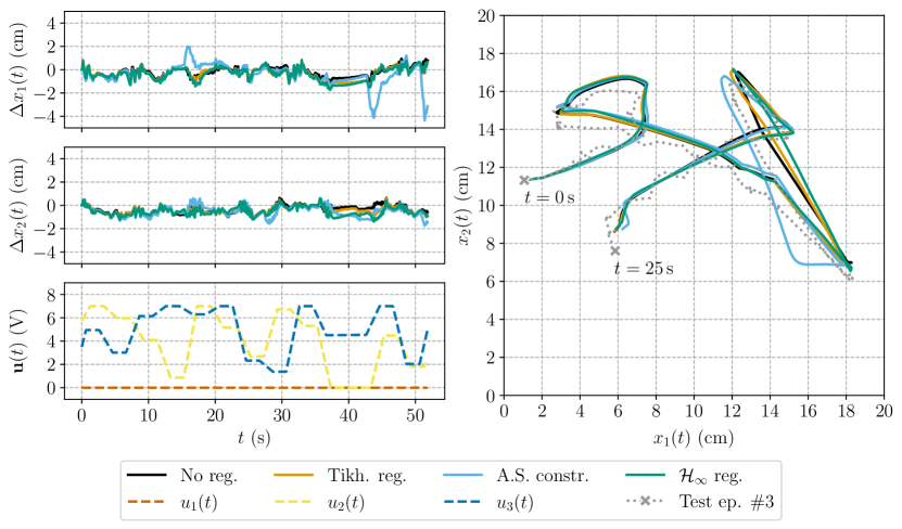
Figure 3: Multi-step prediction error and trajectory plot of the third test episode for Koopman systems approximated from the soft robot dataset. States are recovered and re-lifted between prediction timesteps. All Koopman systems have comparable prediction errors, with the exception of two large error spikes in the system with the asymptotic stability constraint.

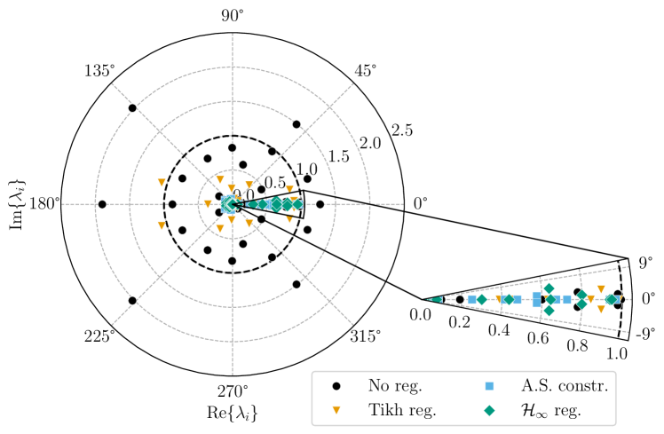
Figure 4: Eigenvalues of Koopman $\mbf{A}$ matrices approximated from the soft robot dataset. EDMD without regularization and EDMD with Tikhonov regularization both identify unstable systems, while the asymptotic stability constraint and $\mathcal{H}_{\infty}$ norm regularizer yield asymptotically stable Koopman systems.

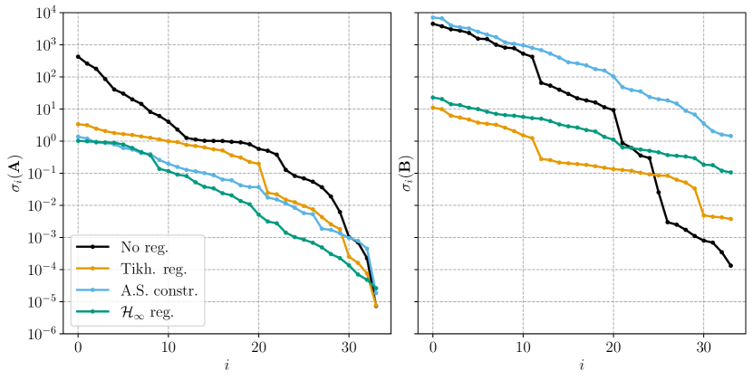
Figure 5: Singular values of Koopman $\mbf{A}$ and $\mbf{B}$ matrices approximated from the soft robot dataset plotted on a logarithmic scale. The $\mbf{A}$ and $\mbf{B}$ matrices computed using unregularized EDMD both have large singular values. EDMD with Tikhonov regularization decreases the singular values of both matrices, but does not yield an asymptotically stable system. With an asymptotic stability constraint, the singular values of $\mbf{A}$ are reduced, but the singular values of $\mbf{B}$ are unaffected and remain large. Using an $\mathcal{H}_{\infty}$ norm regularizer reduces the singular values of both $\mbf{A}$ and $\mbf{B}$ significantly, yielding a better-conditioned Koopman matrix.

Identifying a Koopman representation of a soft robot arm is a particularly interesting problem, as its dynamics are not easily modelled from first principles. The soft robot under consideration consists of two flexible segments with a laser pointer mounted at the end. The laser pointer projects a dot onto a board positioned below the robot. The two states of the system are the Cartesian coordinates of the dot on the board, as measured by a camera. The soft robot arm is actuated by three pressure regulators, each controlled by a voltage. The dot position and control voltages are recorded at $12\text{\,}\mathrm{Hz}$. Thirteen training episodes and four test episodes were recorded in this manner. The third test episode is shown in fig. 3. Photographs of this experimental setup, along with additional details, can be found in [34] and [9].

The lifting functions chosen for the soft robot system consist of a time delay step, followed by a third-order monomial transformation. Although time delays do not, strictly speaking, meet the definition of a lifting function outlined in section 2, they are commonly used in the lifted states of Koopman identification problems [5, 9]. As with the FASTER dataset in section 4, the states and inputs are first normalized. Then, the states and inputs are augmented with their delayed versions, where the delay period is one timestep. Next, all first-, second-, and third-order monomials are computed. Finally, the lifted states are standardized. Since the time delay step occurs before the monomial lifting step, cross-terms including delayed and non-delayed states and inputs occur in the lifted state.

Unregularized EDMD and Tikhonov-regularized EDMD are used as baselines for comparison with the proposed regression methods. Tikhonov regularization improves the numerical conditioning of $\mbf{U}$ by penalizing its squared Frobenius norm [14, 25]. The regularizers used in this section have coefficients of ${\beta=$7.5\text{\times}{10}^{-3}$}$, while the asymptotic stability constraint has a maximum spectral radius of ${\bar{\rho}=0.999}$. Figure 3 shows the multi-step prediction errors of the four Koopman systems for the third test episode of the dataset. The prediction errors are comparable for all four Koopman systems, aside from two large error spikes produced by the system with the asymptotic stability constraint.

One way to compare the resulting Koopman systems is to analyze the eigenvalues of their $\mbf{A}$ matrices. Figure 4 shows that unregularized EDMD and Tikhonov-regularized EDMD produce unstable Koopman systems, even though, as shown in fig. 7, the multi-step prediction errors do not happen to diverge in any test episodes. As expected, EDMD with an $\mathcal{H}_{\infty}$ norm regularizer and EDMD with an asymptotic stability constraint both yield asymptotically stable Koopman systems.

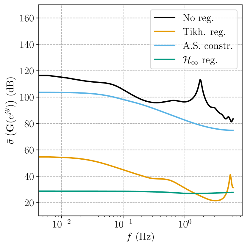
(a)

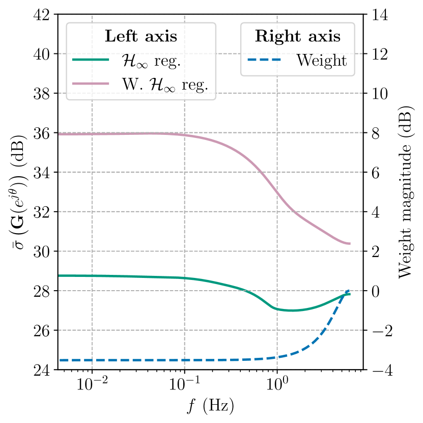
(b)

Figure 6: (6(a)) Bode plot of Koopman systems approximated from the soft robot dataset. The Koopman system identified with unregularized EDMD has high gain, with a resonant peak at a high frequency. EDMD with Tikhonov regularization reduces the system’s gain, but identifies an unstable system and retains an undesirable high-frequency resonant peak in the frequency response. Constraining the asymptotic stability of the system does not significantly reduce the gain compared to the unregularized system. Penalizing the $\mathcal{H}_{\infty}$ norm of the Koopman system reduces its gain at all frequencies without compromising prediction error. (6(b)) Bode plot of unweighted and weighted Koopman systems approximated from the soft robot dataset, along with weighting function. The dashed line representing the weighting function uses the right axis, while the solid lines use the left axis.

While the Koopman system identified with an asymptotic stability constraint is indeed asymptotically stable, the system is not well-conditioned. To see this, consider Figure 5, which shows the singular values of the Koopman $\mbf{A}$ and $\mbf{B}$ matrices. These singular values indicate the sizes of the entries in each matrix. With unregularized EDMD, both matrices have singular values on the order of $10^{3}$. Using Tikhonov regularization decreases the singular values of both $\mbf{A}$ and $\mbf{B}$, though it still yields an unstable system. Constraining the spectral radius of $\mbf{A}$ greatly reduces the singular values of $\mbf{A}$ but increases the singular values of $\mbf{B}$. The numerical conditioning of this Koopman system is arguably worse, as the $\mbf{A}$ and $\mbf{B}$ matrices contain entries of drastically different scales. Regularizing using the $\mathcal{H}_{\infty}$ norm resolves this problem, as it reduces the singular values in both matrices, yielding a better-conditioned, asymptotically stable Koopman system with similar prediction error. The key takeaway is that constraining the spectral radius of $\mbf{A}$ is not sufficient to guarantee a well-conditioned Koopman matrix, as the constraint does not directly impact $\mbf{B}$. Using the $\mathcal{H}_{\infty}$ norm as a regularizer considers the system as a whole, thus impacting both $\mbf{A}$ and $\mbf{B}$, and reducing their entries to reasonable sizes.

Another way to compare the identified Koopman systems is by looking at their frequency responses, which can be found by plotting the maximum singular value of the transfer matrix at each frequency. Figure 6(a) shows the magnitude responses of the four Koopman systems, and paints a similar picture to fig. 5. Unregularized EDMD yields a Koopman system with very high gain and a resonant peak in the upper frequency range. Incorporating Tikhonov regularization reduces the system’s gain, but retains the resonant peak at a high frequency. Constraining the asymptotic stability of the system does not significantly impact the system’s gain, which, given the large singular values of $\mbf{B}$ in fig. 5, is not surprising. However, regularizing using the $\mathcal{H}_{\infty}$ norm directly penalizes the peak of the Bode plot in fig. 6(a), yielding a system with significantly lower gain and similar prediction error.

The $\mathcal{H}_{\infty}$ norm regularizer can be expanded upon by weighting the $\mathcal{H}_{\infty}$ norm using a highpass filter. This weighting function penalizes high gains at high frequencies while allowing higher gains at low frequencies. Penalizing gain at high frequencies is desirable because relevant system dynamics typically occupy low frequencies, while high frequencies are corrupted by measurement noise. Furthermore, causal physical systems have frequency responses that roll off as frequency grows, since it is unrealistic for a system to have infinite gain at infinitely high frequencies. Figure 6(b) demonstrates the impact of weighting the $\mathcal{H}_{\infty}$ norm regularizer with a highpass filter that has a zero at $4\text{\,}\mathrm{Hz}$ and a pole slightly below $6\text{\,}\mathrm{Hz}$. This weighted regularizer yields a Koopman system with high gain at low frequencies and decreasing gain at high frequencies.

Note that fig. 6 shows the frequency response of the Koopman system in the lifted space, which is not the same as the “frequency response of the nonlinear system.” Since the ultimate goal is to design linear controllers in the lifted space, only the frequency response of the Koopman system in the lifted space and the corresponding $\mathcal{H}_{\infty}$ norm are relevant.

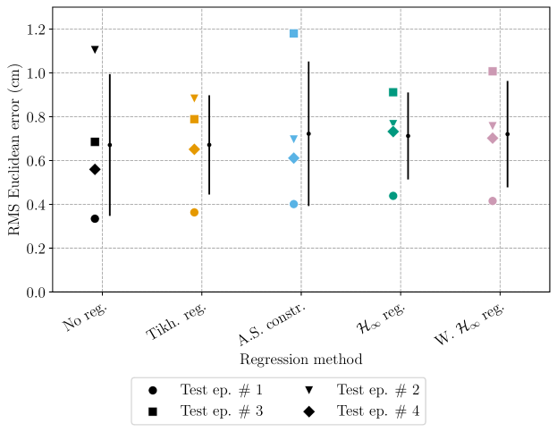
Figure 7: RMS Euclidean errors of Koopman systems approximated from the soft robot dataset. Error bars indicate mean and standard deviation of RMS error over the four test episodes. In terms of mean error, all identified Koopman systems perform similarly well. However, the system identified using $\mathcal{H}_{\infty}$ norm regularizer performed more consistently throughout the test set.

In fig. 7, the multi-step prediction errors of the five identified Koopman systems are compared across each episode in the test set. Given that the laser pointer dot projected by the soft robot moves within a circle of radius $10\text{\,}\mathrm{cm}$, it’s practically meaningless to distinguish each method based on mean prediction error alone. However, the distribution of each identified system’s prediction errors across the test set clearly highlights the importance of regularization. The Tikhonov regularizer, $\mathcal{H}_{\infty}$ norm regularizer, and weighted $\mathcal{H}_{\infty}$ norm regularizer lead to systems with smaller standard deviations in the RMS error over the test set. In contrast, EDMD without regularization and EDMD with an asymptotic stability constraint lead to systems that perform inconsistently over the test set. Comparing standard deviations indicates that the regularized systems generalize better to previously unseen data, with the $\mathcal{H}_{\infty}$ norm regularizer performing most consistently over the four test episodes.

The results in this section highlight the desirable properties of the proposed $\mathcal{H}_{\infty}$ norm regularizers. While all systems have comparable RMS prediction errors on the test set, unregularized EDMD results in an unstable, poorly conditioned Koopman system with large gain. While Tikhonov regularization improves numerical conditioning, the resulting system is still unstable. Conversely, constraining the asymptotic stability of the system does not improve it numerical properties. Only the $\mathcal{H}_{\infty}$ norm regularizers guarantee asymptotic stability while improving the numerical conditioning of the system. These key results are summarized in table 1, which also highlights the difference between the unweighted and weighted $\mathcal{H}_{\infty}$ norm regularizers. Weighting the $\mathcal{H}_{\infty}$ norm regularizer further improves the condition numbers of $\mbf{A}$ and $\mbf{B}$.

Table 1: Comparison of regression methods through the condition numbers of their Koopman matrices and asymptotic stability guarantees. Only the $\mathcal{H}_{\infty}$ regularizers guarantee asymptotic stability while significantly improving the condition number of the Koopman matrices. In this case, weighting the $\mathcal{H}_{\infty}$ norm further improves $\mathrm{cond}(\mbf{A})$ and $\mathrm{cond}(\mbf{B})$.

regression method	$\mathrm{cond}(\mbf{A})$	$\mathrm{cond}(\mbf{B})$	asymptotic stability
no regularization	$5.77\times 10^{7}$	$3.40\times 10^{7}$	no
Tikhonov regularization	$4.39\times 10^{5}$	$2.90\times 10^{3}$	no
asymptotic stability constraint	$7.32\times 10^{4}$	$4.87\times 10^{3}$	yes
$\mathcal{H}_{\infty}$ regularization	$3.87\times 10^{4}$	$2.14\times 10^{2}$	yes
weighted $\mathcal{H}_{\infty}$ regularization	$1.69\times 10^{3}$	$5.43\times 10^{1}$	yes

6 Reducing the Size of the Regression Problem

As the number of lifting functions required grows, so does the size of the optimization problem. With several hundred lifting functions, finding a solution can take days and consume an intractable amount of memory. To combat this limitation, an approach reminiscent of DMDc is now presented.

6.1 DMD with control

DMD with control [17] reduces the dimension of the Koopman matrix regression problem when the dataset contains many more lifted states than time snapshots (i.e. , ${p\gg q}$) [12, §10.3]. In DMDc, the Koopman matrix is projected onto the left singular vectors of $\bm{\Theta}_{+}$. The size of the problem is then controlled by retaining only the $\hat{r}$ largest singular values in the SVD. Consider the truncated singular value decomposition ${\bm{\Theta}_{+}\approx\hat{\mbf{Q}}\hat{\bm{\Sigma}}\hat{\mbf{Z}}^{\mathsf{T}}}$, where ${\hat{\mbf{Q}}\in\mathbb{R}^{p_{\vartheta}\times\hat{r}}}$, ${\hat{\bm{\Sigma}}\in\mathbb{R}^{\hat{r}\times\hat{r}}}$, and ${\hat{\mbf{Z}}\in\mathbb{R}^{q\times\hat{r}}}$. Instead of solving for ${\mbf{U}=\begin{bmatrix}\mbf{A}&\mbf{B}\end{bmatrix}}$, the regression problem is written in terms of [17]

$$\hat{\mbf{U}}=\begin{bmatrix}\hat{\mbf{Q}}^{\mathsf{T}}\mbf{A}\hat{\mbf{Q}}&\hat{\mbf{Q}}^{\mathsf{T}}\mbf{B}\end{bmatrix}=\hat{\mbf{Q}}^{\mathsf{T}}\mbf{U}\!\begin{bmatrix}\hat{\mbf{Q}}&\mbf{0}\\ \mbf{0}&\mbf{1}\end{bmatrix},$$ (47)

where ${\hat{\mbf{U}}\in\mathbb{R}^{\hat{r}\times\hat{r}+p_{\upsilon}}}$ is significantly smaller than ${\mbf{U}\in\mathbb{R}^{p_{\vartheta}\times p}}$. The least-squares solution to the Koopman matrix eq. 14 can be written as

$$\mbf{U}=\bm{\Theta}_{+}\tilde{\mbf{Z}}\tilde{\bm{\Sigma}}^{\dagger}\tilde{\mbf{Q}}^{\mathsf{T}},$$ (48)

where ${\bm{\Psi}\approx\tilde{\mbf{Q}}\tilde{\bm{\Sigma}}\tilde{\mbf{Z}}^{\mathsf{T}}}$. The number of singular values retained in this SVD is denoted $\tilde{r}$. Thus ${\tilde{\mbf{Q}}\in\mathbb{R}^{p\times\tilde{r}}}$, ${\tilde{\bm{\Sigma}}\in\mathbb{R}^{\tilde{r}\times\tilde{r}}}$, and ${\tilde{\mbf{Z}}\in\mathbb{R}^{q\times\tilde{r}}}$. The standard solution to the DMDc problem is obtained by substituting eq. 48 into eq. 47, yielding

$$\hat{\mbf{U}}=\hat{\mbf{Q}}^{\mathsf{T}}\bm{\Theta}_{+}\tilde{\mbf{Z}}\tilde{\bm{\Sigma}}^{\dagger}\tilde{\mbf{Q}}^{\mathsf{T}}\begin{bmatrix}\hat{\mbf{Q}}&\mbf{0}\\ \mbf{0}&\mbf{1}\end{bmatrix}.$$ (49)

The SVD dimensions $\hat{r}$ and $\tilde{r}$ are a design choice. A common approach is the hard-thresholding algorithm described in [35]. Note that typically ${\hat{r}<\tilde{r}}$ [12, §6.1.3].

6.2 LMI reformulation of DMDc

To reformulate DMDc as a convex optimization problem with LMI constraints, the cost function is rewritten in terms of $\hat{\mbf{U}}$ instead of $\mbf{U}$. Recall that the rescaled Koopman cost function eq. 17 can be written as

$$\min J(\mbf{U})=\frac{1}{q}{\mathrm{tr}}{\left(\bm{\Theta}_{+}\bm{\Theta}_{+}^{\mathsf{T}}-{\mathrm{He}\!\left\{\mbf{U}\bm{\Psi}\bm{\Theta}_{+}^{\mathsf{T}}\right\}}+\mbf{U}\bm{\Psi}\bm{\Psi}^{\mathsf{T}}\mbf{U}^{\mathsf{T}}\right)}.$$ (50)

With the introduction of a slack variable, eq. 50 becomes [27, §2.15.1]

$$\min\; J(\mbf{U},\mbf{W})=\frac{1}{q}{\mathrm{tr}}{(\mbf{W})}$$ (51)

$$\mathrm{s.t.}\; \mbf{W}>0,\quad\bm{\Theta}_{+}\bm{\Theta}_{+}^{\mathsf{T}}-{\mathrm{He}\!\left\{\mbf{U}\bm{\Psi}\bm{\Theta}_{+}^{\mathsf{T}}\right\}}+\mbf{U}\bm{\Psi}\bm{\Psi}^{\mathsf{T}}\mbf{U}^{\mathsf{T}}<\mbf{W}.$$ (52)

Substituting the SVDs of $\bm{\Theta}_{+}$ and $\bm{\Psi}$ into the optimization problem yields

$$\min\; J(\mbf{U},\mbf{W})=\frac{1}{q}{\mathrm{tr}}{(\mbf{W})}$$ (53)

$$\mathrm{s.t.}\; \mbf{W}>0,\quad\hat{\mbf{Q}}\hat{\bm{\Sigma}}^{2}\hat{\mbf{Q}}^{\mathsf{T}}-{\mathrm{He}\!\left\{\mbf{U}\tilde{\mbf{Q}}\tilde{\bm{\Sigma}}\tilde{\mbf{Z}}^{\mathsf{T}}\hat{\mbf{Z}}\hat{\bm{\Sigma}}\hat{\mbf{Q}}^{\mathsf{T}}\right\}}+\mbf{U}\tilde{\mbf{Q}}\tilde{\bm{\Sigma}}^{2}\tilde{\mbf{Q}}^{\mathsf{T}}\mbf{U}^{\mathsf{T}}<\mbf{W}.$$ (54)

Next, consider the projection of eq. 53 and eq. 54 onto the column space of $\hat{\mbf{Q}}$, denoted $\mathcal{R}(\hat{\mbf{Q}})$. Recall that $\mbf{W}>0$ is equivalent to

$$\bm{\vartheta}^{\mathsf{T}}\mbf{W}\bm{\vartheta}>0,\ \forall\bm{\vartheta}\neq\mbf{0}\in\mathbb{R}^{p_{\vartheta}\times 1}.$$ (55)

Since eq. 55 holds over all of $\mathbb{R}^{p_{\vartheta}\times 1}$, it must also hold over the subspace $\mathcal{R}(\hat{\mbf{Q}})$. Let the vectors in $\mathcal{R}(\hat{\mbf{Q}})$ be parameterized by

$$\bm{\vartheta}=\hat{\mbf{Q}}\hat{\bm{\vartheta}},$$ (56)

where ${\hat{\bm{\vartheta}}\in\mathbb{R}^{\hat{r}\times 1}}$. Substituting eq. 56 into eq. 55 yields

$$\hat{\bm{\vartheta}}^{\mathsf{T}}\hat{\mbf{Q}}^{\mathsf{T}}\mbf{W}\hat{\mbf{Q}}\hat{\bm{\vartheta}}>0,\ \forall\hat{\bm{\vartheta}}\neq\mbf{0}\in\mathbb{R}^{\hat{r}\times 1},$$ (57)

which is equivalent to

$$\hat{\mbf{W}}=\hat{\mbf{Q}}^{\mathsf{T}}\mbf{W}\hat{\mbf{Q}}>0$$ (58)

over $\mathcal{R}(\hat{\mbf{Q}})$. Applying the same logic to eq. 54 yields

$$\hat{\bm{\Sigma}}^{2}-{\mathrm{He}\!\left\{\hat{\mbf{Q}}^{\mathsf{T}}\mbf{U}\tilde{\mbf{Q}}\tilde{\bm{\Sigma}}\tilde{\mbf{Z}}^{\mathsf{T}}\hat{\mbf{Z}}\hat{\bm{\Sigma}}\right\}}+\hat{\mbf{Q}}^{\mathsf{T}}\mbf{U}\tilde{\mbf{Q}}\tilde{\bm{\Sigma}}^{2}\tilde{\mbf{Q}}^{\mathsf{T}}\mbf{U}^{\mathsf{T}}\hat{\mbf{Q}}<\hat{\mbf{W}},$$ (59)

where the fact that ${\hat{\mbf{Q}}^{\mathsf{T}}\hat{\mbf{Q}}=\mbf{1}}$ has been used.

To further simplify the problem, it is advantageous to rewrite eq. 53 in terms of $\hat{\mbf{W}}$. To accomplish this, first recall that the trace of a matrix is equal to the sum of its eigenvalues. The eigenvalue problem for $\mbf{W}$ is

$$\mbf{W}\mbf{v}_{i}=\lambda_{i}\mbf{v}_{i}.$$ (60)

Projecting eq. 60 onto $\mathcal{R}(\hat{\mbf{Q}})$ by substituting ${\mbf{v}_{i}=\hat{\mbf{Q}}\hat{\mbf{v}}_{i}}$, then premultiplying the result by $\hat{\mbf{Q}}^{\mathsf{T}}$, yields

$$\hat{\mbf{Q}}^{\mathsf{T}}\mbf{W}\hat{\mbf{Q}}\hat{\mbf{v}}_{i}=\lambda_{i}\hat{\mbf{v}}_{i}.$$ (61)

Thus, $\mbf{W}$ and $\hat{\mbf{W}}$ share the same eigenvalues for eigenvectors in $\mathcal{R}(\hat{\mbf{Q}})$, which indicates that minimizing ${\mathrm{tr}}(\hat{\mbf{W}})$ is equivalent to minimizing ${\mathrm{tr}}(\mbf{W})$ in that subspace.

The full regression problem projected onto $\mathcal{R}(\hat{\mbf{Q}})$ is therefore

$$\min\; J(\mbf{U},\hat{\mbf{W}})=\frac{1}{q}{\mathrm{tr}}{(\hat{\mbf{W}})}$$ (62)

$$\mathrm{s.t.}\; \hat{\mbf{W}}>0,\quad\hat{\bm{\Sigma}}^{2}-{\mathrm{He}\!\left\{\hat{\mbf{Q}}^{\mathsf{T}}\mbf{U}\tilde{\mbf{Q}}\tilde{\bm{\Sigma}}\tilde{\mbf{Z}}^{\mathsf{T}}\hat{\mbf{Z}}\hat{\bm{\Sigma}}\right\}}+\hat{\mbf{Q}}^{\mathsf{T}}\mbf{U}\tilde{\mbf{Q}}\tilde{\bm{\Sigma}}^{2}\tilde{\mbf{Q}}^{\mathsf{T}}\mbf{U}^{\mathsf{T}}\hat{\mbf{Q}}<\hat{\mbf{W}}.$$ (63)

Substituting $\hat{\mbf{U}}$ from eq. 47 into the optimization problem yields

$$\min\; J(\hat{\mbf{U}},\hat{\mbf{W}})=\frac{1}{q}{\mathrm{tr}}{(\hat{\mbf{W}})}$$ (64)

$$\mathrm{s.t.}\; \hat{\mbf{W}}>0,\quad\hat{\bm{\Sigma}}^{2}-{\mathrm{He}\!\left\{\hat{\mbf{U}}\bar{\mbf{Q}}\tilde{\bm{\Sigma}}\tilde{\mbf{Z}}^{\mathsf{T}}\hat{\mbf{Z}}\hat{\bm{\Sigma}}\right\}}+\hat{\mbf{U}}\bar{\mbf{Q}}\tilde{\bm{\Sigma}}^{2}\bar{\mbf{Q}}^{\mathsf{T}}\hat{\mbf{U}}^{\mathsf{T}}<\hat{\mbf{W}},$$ (65)

where

$$\bar{\mbf{Q}}=\begin{bmatrix}\hat{\mbf{Q}}&\mbf{0}\\ \mbf{0}&\mbf{1}\end{bmatrix}^{\mathsf{T}}\tilde{\mbf{Q}}.$$ (66)

Applying the Schur complement to eq. 65 yields the LMI formulation of DMDc,

$$\min\; J(\hat{\mbf{U}},\hat{\mbf{W}})=\frac{1}{q}{\mathrm{tr}}{(\hat{\mbf{W}})}$$ (67)

$$\mathrm{s.t.}\; \hat{\mbf{W}}>0,\quad\begin{bmatrix}-\hat{\mbf{W}}+\hat{\bm{\Sigma}}^{2}-{\mathrm{He}\!\left\{\hat{\mbf{U}}\bar{\mbf{Q}}\tilde{\bm{\Sigma}}\tilde{\mbf{Z}}^{\mathsf{T}}\hat{\mbf{Z}}\hat{\bm{\Sigma}}\right\}}&\hat{\mbf{U}}\bar{\mbf{Q}}\tilde{\bm{\Sigma}}\\ \tilde{\bm{\Sigma}}\bar{\mbf{Q}}^{\mathsf{T}}\hat{\mbf{U}}^{\mathsf{T}}&-\mbf{1}\end{bmatrix}<0.$$ (68)

This is now a significantly smaller optimization problem, as its size is controlled by the truncation of the SVD of $\bm{\Theta}_{+}$. Reducing the first dimension of $\hat{\mbf{U}}$ also reduces the dimension of the slack variable $\hat{\mbf{W}}$.

6.3 Constraints and regularization

The projection in eq. 56 defines a new Koopman system,

$$\hat{\bm{\vartheta}}_{k+1} =\hat{\mbf{A}}\hat{\bm{\vartheta}}_{k}+\hat{\mbf{B}}\bm{\upsilon}_{k},$$ (69)

$$\bm{\zeta}_{k} =\hat{\mbf{C}}\hat{\bm{\vartheta}}_{k}+\mbf{D}\bm{\upsilon}_{k},$$ (70)

where $\hat{\mbf{C}}=\mbf{C}\hat{\mbf{Q}}$. The asymptotic stability constraint discussed in section 4 and the $\mathcal{H}_{\infty}$ norm regularizers discussed in section 5 can be equally applied to the projected system in eq. 69 and eq. 70 to ensure that the projected system of smaller dimension has the desired stability and frequency response characteristics.

6.4 Experimental results

The properties of the asymptotic stability constraint from section 4 and the $\mathcal{H}_{\infty}$ norm regularizer from section 5 are now compared when applied to the EDMD and DMDc regression problems. The same dataset and experimental setup as section 5 is used here.

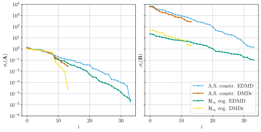
Figure 8: Singular values of Koopman $\mbf{A}$ and $\mbf{B}$ matrices approximated from the soft robot dataset using EDMD and DMDc regressors. Singular values smaller than $10^{-12}$ are not shown. Note the logarithmic scale. While the EDMD methods retain all 34 singular values, the DMDc methods truncate all but the first 14. The singular values retained by the DMDc methods are close to the corresponding singular values computed by the EDMD methods.

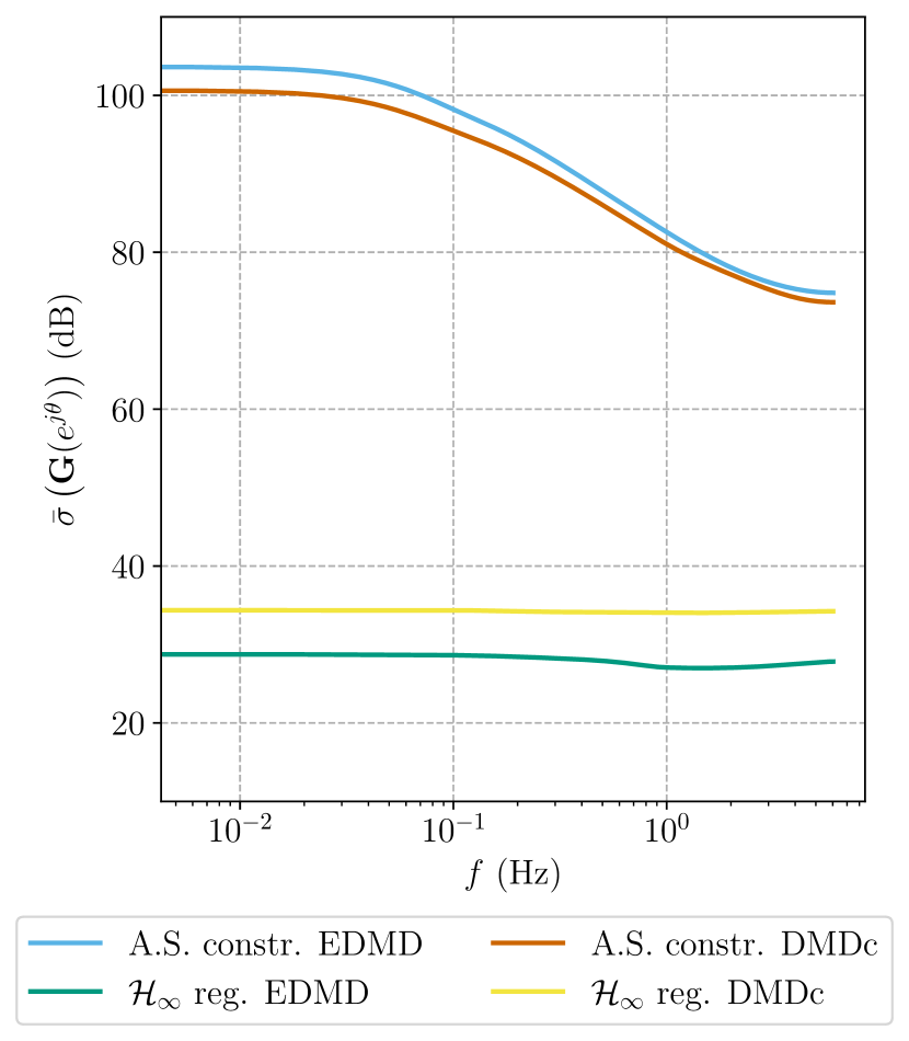
(a)

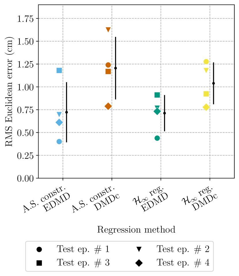
(b)

Figure 9: (9(a)) Bode plots of Koopman systems approximated from the soft robot dataset using EDMD and DMDc regressors. The DMDc methods preserve the frequency responses of the corresponding systems identified with the EDMD methods. (9(b)) RMS Euclidean errors of Koopman systems approximated from the soft robot dataset using EDMD and DMDc regressors. Error bars indicate standard deviation of RMS error over the four test episodes. Since the DMDc methods identify reduced-order Koopman models of the system, they have larger mean errors. However, the $\mathcal{H}_{\infty}$ norm regularizer still significantly reduces the standard deviation.

An important decision in the DMDc algorithm is the choice of singular value truncation method. Optimal hard singular value truncation [35] is used to determine $\hat{r}$, while $\tilde{r}$ is left at full rank. For the soft robot dataset, the optimal hard truncation algorithm retains only 14 of the 34 singular values of $\mbf{A}$. Figure 8 demonstrates that the DMDc methods indeed reduce the dimensionality of the problem, while also showing that the remaining singular values are close to their EDMD counterparts. Figure 9(a) shows that the frequency responses of the original Koopman systems are preserved by the DMDc methods. In spite of their reduced dimensionality, the Koopman systems identified with DMDc retain their frequency domain properties.

In fig. 9(b), the RMS Euclidean errors of the EDMD and DMDc methods with asymptotic stability constraints and $\mathcal{H}_{\infty}$ norm regularization are summarized. Since the Koopman systems identified by the DMDc methods are of a lower order, their mean prediction error is higher than that of the EDMD methods. However, the $\mathcal{H}_{\infty}$ norm regularizer retains its benefit of improving prediction consistency. Furthermore, as demonstrated by fig. 9(a), the frequency response properties of the EDMD regression methods are preserved by the reduced-order DMDc models.

Note that, in one case, the Koopman system identified using stability-constrained DMDc diverged due to poor numerical conditioning. This short segment of the dataset was omitted throughout the paper to allow for a more fair comparison between regression methods. This finding highlights the advantages of the $\mathcal{H}_{\infty}$ regularization method in identifying numerically well-conditioned Koopman matrices.

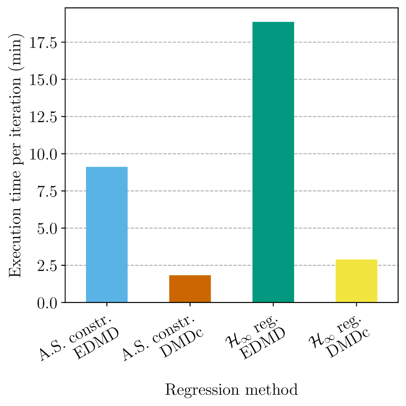
(a)

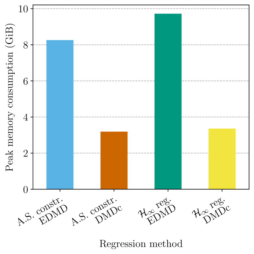
(b)

Figure 10: (10(a)) Execution time per iteration and (10(b)) peak memory consumption of EDMD and DMDc regression methods using the soft robot dataset. The DMDc methods run significantly faster and consume less memory than the EDMD methods. Tests were run on a PC with an Intel Core i7-10700K processor using the MOSEK solver.

The most important advantage of the DMDc regression methods is their computational savings when many lifting functions are required. The long execution times of the EDMD methods, along with their high memory consumption, make cross-validation impractical. Figure 10 demonstrates the significant resource savings provided by the DMDc methods in both execution time and peak memory consumption. Memory consumption is of particular importance when running multiple instances of a regressor in a multi-process cross-validation scheme. The DMDc regression methods presented provide significant computational savings while still retaining the frequency-domain characteristics of their EDMD counterparts. In spite of their higher mean prediction error, it is often worthwhile to leverage them for Koopman operator identification, particularly when hyperparameter optimization is a priority.

7 Conclusion

Approximating the Koopman matrix using linear regression proves challenging as lifting function complexity increases. Even small problems can become ill-conditioned when many lifting functions are required for an accurate fit. Viewing the problem from a systems perspective, where system inputs pass through dynamics and lead to outputs, provides multiple avenues to enforce asymptotic stability and penalize large input-output gains in the system, thus ensuring improved numerical conditioning. In particular, regularizing the regression problem with the $\mathcal{H}_{\infty}$ norm provides the opportunity to tune the regularization process in the frequency domain using weighting functions. The significant performance savings presented by the DMDc-based regression methods allow the $\mathcal{H}_{\infty}$ norm regularizer to be applied to much larger systems while still remaining tractable.

The nonconvex optimization problems required to use the asymptotic stability constraint and $\mathcal{H}_{\infty}$ norm regularizers limit their applicability to practical problems. Future research will address this limitation by making use of more efficient BMI solution methods, including Iterative Convex Overbounding [36] and branch-and-bound methods [37]. Although the use of the $\mathcal{H}_{\infty}$ norm [27, §3.2] as a regularizer is explored in this paper, any system norm, like the $\mathcal{H}_{2}$ norm [27, §3.3] or a mixed $\mathcal{H}_{2}$ norm [27, §3.5], can be used. The unique properties of system norms prove useful in addressing the numerical challenges associated with approximating the Koopman operator from data, and will be explored further in future work.

The methods presented in this paper and its predecessor [25] are implemented in release v1.0.4 of pykoop, the authors’ open source Koopman operator identification library [38]. The code required to reproduce the plots in this paper is available in a companion repository at https://github.com/decarsg/system_norm_koopman, release v1.0.3.

Both authors conceived of the research and performed the formal analysis. S.D. wrote the software, performed the experiments, and prepared the visualizations. J.R.F. supervised the research, formulated its high-level objectives, and assisted with detailed derivations.

The authors declare that they have no competing interests.

This work was supported by the Mecademic Inc. through the Mitacs Accelerate program, and by the Natural Sciences and Engineering Research Council of Canada (NSERC), the National Research Council of Canada (NRC), the Toyota Research Institute, the National Science Foundation Career Award [grant number 1751093], and the Office of Naval Research [grant number N00014-18-1-2575].

The authors thank Daniel Bruder, Xun Fu, and Ram Vasudevan for graciously providing the soft robot dataset used in this research. The authors also acknowledge Doug Shi-Dong, Robyn Fortune, Shaowu Pan, Karthik Duraisamy, and Matthew M. Peet for productive discussions about regularization techniques, the Koopman operator, and methods for handling BMI constraints.

References

- [1] Koopman BO. 1931 Hamiltonian systems and transformations in Hilbert space. Proc. Nat. Acad. Sci. 17, 315–318.
- [2] Mezić I. 2019 Spectrum of the Koopman Operator, Spectral Expansions in Functional Spaces, and State-Space Geometry. J. Nonlinear Sci. 30, 2091–2145.
- [3] Budišić M, Mohr R, Mezić I. 2012 Applied Koopmanism. Chaos 22.
- [4] Mauroy A, Mezić I, Susuki Y, editors. 2020 The Koopman Operator in Systems and Control. Cham, Switzerland: Springer.
- [5] Korda M, Mezić I. 2018 Linear predictors for nonlinear dynamical systems: Koopman operator meets model predictive control. Automatica 93, 149–160.
- [6] Otto SE, Rowley CW. 2021 Koopman Operators for Estimation and Control of Dynamical Systems. Annu. Rev. Control, Robot., Auton. Syst. 4, 59–87.
- [7] Abraham I, Murphey TD. 2019 Active Learning of Dynamics for Data-Driven Control Using Koopman Operators. IEEE Trans. Robot. 35, 1071–1083.
- [8] Mamakoukas G, Castano M, Tan X, Murphey T. 2019 Local Koopman Operators for Data-Driven Control of Robotic Systems. In Proc. Robot.: Sci. Syst. XV Freiburg im Breisgau, Germany.
- [9] Bruder D, Gillespie B, Remy CD, Vasudevan R. 2019 Modeling and Control of Soft Robots Using the Koopman Operator and Model Predictive Control. In Proc. Robot.: Sci. Syst. XV Freiburg im Breisgau, Germany.
- [10] Uchida D, Yamashita A, Asama H. 2021 Data-Driven Koopman Controller Synthesis Based on the Extended Norm Characterization. IEEE Contr. Syst. Lett. 5, 1795–1800.
- [11] Abraham I, de la Torre G, Murphey T. 2017 Model-Based Control Using Koopman Operators. In Proc. Robot.: Sci. Syst. XIII Cambridge, MA.
- [12] Kutz NJ, Brunton SL, Brunton BW, Proctor JL. 2016 Dynamic Mode Decomposition: Data-Driven Modeling of Complex Systems. Philadelphia, PA: SIAM.
- [13] Mamakoukas G, Abraham I, Murphey TD. 2020 Learning Data-Driven Stable Koopman Operators. arXiv:2005.04291v1 [cs.RO].
- [14] Tikhonov AN, Goncharsky A, Stepanov VV, Yagola AG. 1995 Numerical Methods for the Solution of Ill-Posed Problems. Dordrecht, Netherlands: Springer.
- [15] Tibshirani R. 1996 Regression Shrinkage and Selection Via the Lasso. J. Roy. Statistical Soc.: Ser. B 58, 267–288.
- [16] Williams MO, Kevrekidis IG, Rowley CW. 2015 A Data–Driven Approximation of the Koopman Operator: Extending Dynamic Mode Decomposition. J. Nonlinear Sci. 25, 1307–1346.
- [17] Proctor JL, Brunton SL, Kutz JN. 2014 Dynamic mode decomposition with control. arXiv:1409.6358v1 [math.OC].
- [18] Sznaier M. 2021 A Convex Optimization Approach to Learning Koopman Operators. arXiv:2102.03934v1 [eess.SY].
- [19] Hara K, Inoue M, Sebe N. 2020 Learning Koopman Operator under Dissipativity Constraints. IFAC-PapersOnLine 53, 1169–1174.
- [20] Lacy SL, Bernstein DS. 2002 Subspace identification with guaranteed stability using constrained optimization. In Proc. 2002 Amer. Control Conf. Anchorage, AK.
- [21] Hoagg JB, Lacy SL, Erwin RS, Bernstein DS. 2004 First-order-hold sampling of positive real systems and subspace identification of positive real models. In Proc. 2004 Amer. Control Conf. Boston, MA.
- [22] Siddiqi SM, Boots B, Gordon GJ. 2008 A Constraint Generation Approach to Learning Stable Linear Dynamical Systems. Technical report Defense Technical Information Center.
- [23] Mamakoukas G, Xherija O, Murphey T. 2020 Memory-Efficient Learning of Stable Linear Dynamical Systems for Prediction and Control. Advances Neural Inf. Process. Syst. 33, 13527–13538.
- [24] Gillis N, Karow M, Sharma P. 2020 A note on approximating the nearest stable discrete-time descriptor systems with fixed rank. Appl. Numer. Math. 148, 131–139.
- [25] Dahdah S, Forbes JR. 2021 Linear Matrix Inequality Approaches to Koopman Operator Approximation. arXiv:2102.03613v2 [eess.SY].
- [26] Bruder D, Fu X, Vasudevan R. 2021 Advantages of Bilinear Koopman Realizations for the Modeling and Control of Systems With Unknown Dynamics. IEEE Trans. Robot. Autom. 6, 4369–4376.
- [27] Caverly RJ, Forbes JR. 2019 LMI Properties and Applications in Systems, Stability, and Control Theory. arXiv:1903.08599v3 [cs.SY].
- [28] El Ghaoui L, Niculescu SI. 2000 Advances in Linear Matrix Inequality Methods in Control. SIAM.
- [29] Doroudchi A, Shivakumar S, Fisher RE, Marvi H, Aukes D, He X, Berman S, Peet MM. 2018 Decentralized Control of Distributed Actuation in a Segmented Soft Robot Arm. In 2018 IEEE Conf. Decision Control Miami Beach, FL.
- [30] Fortune R, Beltempo CA, Forbes JR. 2019 System Identification and Feedforward Control of a Fatigue Structural Testing Rig: The Single Actuator Case. IFAC-PapersOnLine 52, 382–387.
- [31] James G, Witten D, Hastie T, Tibshirani R. 2013 An Introduction to Statistical Learning. New York, NY: Springer.
- [32] Zhou K, Doyle JC, Glover K. 1995 Robust and Optimal Control. Englewood Cliffs, NJ: Prentice Hall.
- [33] Green M, Limebeer DJN. 1994 Linear Robust Control. London, England: Prentice Hall.
- [34] Bruder D, Fu X, Gillespie RB, Remy CD, Vasudevan R. 2021 Data-Driven Control of Soft Robots Using Koopman Operator Theory. IEEE Trans. Robot. 37, 948–961.
- [35] Gavish M, Donoho DL. 2014 The Optimal Hard Threshold for Singular Values is . IEEE Trans. Inf. Theory 60, 5040–5053.
- [36] Warner E, Scruggs J. 2017 Iterative Convex Overbounding Algorithms for BMI Optimization Problems. IFAC-PapersOnLine 50, 10449–10455.
- [37] VanAntwerp JG, Braatz RD. 2000 A tutorial on linear and bilinear matrix inequalities. J. Process Control 10, 363–385.
- [38] Dahdah S, Forbes JR. 2021 decarsg/pykoop. https://github.com/decarsg/pykoop.