Dynamic Feature Alignment for
Semi-supervised Domain Adaptation

Abstract

Most research on domain adaptation has focused on the purely unsupervised setting, where no labeled examples in the target domain are available. However, in many real-world scenarios, a small amount of labeled target data is available and can be used to improve adaptation. We address this semi-supervised setting and propose to use dynamic feature alignment to address both inter- and intra-domain discrepancy. Unlike previous approaches, which attempt to align source and target features within a mini-batch, we propose to align the target features to a set of dynamically updated class prototypes, which we use both for minimizing divergence and pseudo-labeling. By updating based on class prototypes, we avoid problems that arise in previous approaches due to class imbalances. Our approach, which doesn’t require extensive tuning or adversarial training, significantly improves the state of the art for semi-supervised domain adaptation. We provide a quantitative evaluation on two standard datasets, DomainNet and Office-Home, and performance analysis. Project Page: https://mvrl.github.io/DFA

1 Introduction

Deep neural networks have achieved impressive performance on a wide range of tasks, including image classification, semantic segmentation, and object detection. However, models often generalize poorly to new domains, such as when a model trained on indoor imagery is used to interpret an outdoor image. Domain Adaptation (DA) methods aim to take a model trained on a label-rich source domain and make it generalize well to a label-scarce target domain. Recently, most studies on domain adaptation have focused on the Unsupervised Domain Adaptation (UDA) setting, in which no labeled target data is available. However, in real-world scenarios there is often a small amount of labeled target data available: the Semi-Supervised Domain Adaptation (SSDA) setting. Recent works [Kim and Kim(), Saito et al.()Saito, Kim, Sclaroff, Darrell, and Saenko] demonstrate that directly applying UDA methods on the semi-supervised setting can actually hurt performance. Therefore, finding a way to effectively use the small amount of labeled target imagery is an important problem. We propose a novel approach that is tailored to the SSDA setting.

In addition to poor generalization in terms of model performance, the intermediate features for source and target domain inputs often display a significant domain shift. This motivates approaches that use feature alignment strategies [Ganin and Lempitsky(), Cao et al.()Cao, Long, and Wang, Dong et al.()Dong, Cong, Sun, Liu, and Xu, Dong et al.(2020)Dong, Cong, Sun, Zhong, and Xu, Hoffman et al.()Hoffman, Tzeng, Park, Zhu, Isola, Saenko, Efros, and Darrell, Zhu et al.(2017)Zhu, Park, Isola, and Efros, Jiang et al.()Jiang, Wu, Han, Shao, Qi, and Li, Saito et al.()Saito, Kim, Sclaroff, Darrell, and Saenko] to minimize the distances between source and target distributions. These methods address the shift between source and unlabeled target samples but ignore the shift within the target domain brought by the small number of labeled target samples. A recent work APE [Kim and Kim()] addresses this issue as intra-domain discrepancy, and proposes three schemes—attraction, perturbation, and exploration, to alleviate this discrepancy. Attraction is used to push the unlabeled features to the labeled feature distribution. Perturbation aims to move both labeled and unlabeled target features to their intermediate regions to minimize the gap in between. Exploration is complementary to the other two schemes by selectively aligning unlabeled target features to the source.

Due to the imbalance between the large amount of labeled source data and the small amount of labeled target data as well as the class imbalance (e.g. the existence of long-tail classes), a random mini-batch of aligned features can not always represent the true distribution of the data. Therefore, the alignment of unlabeled features can be inaccurate. Moreover, errors can be accumulated when incorrectly predicted unlabeled samples are selected to be used for pseudo-label training during exploration.

Considering the concerns mentioned above, we propose a novel Dynamic Feature Alignment (DFA) framework for the SSDA problem. Instead of directly aligning the unaligned target features to the aligned features within a mini-batch, we propose to align the unlabeled target features to a set of dynamically updated class prototypes, which are stored in a dynamic memory bank $\mathcal{B}$. To utilize these prototypes for pseudo-labeling, we selectively collect unlabeled samples based on their distances to class prototypes and their prediction entropy. We evaluate our method on standard domain adaptation benchmarks, including DomainNet and Office-Home, and results show that our method achieves significant improvement over the state of the art in both the 1-shot and 3-shot settings.

2 Related Work

We introduce related work in unsupervised and semi-supervised domain adaptation and describe their relationship to our approach.

2.1 Unsupervised Domain Adaptation

UDA is a machine learning technique that trains a model on one or more source domains and attempts to make the model generalize well on a different but related target domain [Ben-David et al.(2010)Ben-David, Blitzer, Crammer, Kulesza, Pereira, and Vaughan, Redko et al.(2019)Redko, Morvant, Habrard, Sebban, and Bennani]. One of the key challenges of UDA is to mitigate the domain shift (or distribution shift) between the source and target domains. In general, three types of techniques can be used [Wang and Deng(2018), Wilson and Cook(2020)]: (1) adversarial, (2) reconstruction based, and (3) divergence based.

The adversarial methods achieve domain adaptation by using adversarial training [Dong et al.(2020)Dong, Cong, Sun, Zhong, and Xu, Hoffman et al.()Hoffman, Tzeng, Park, Zhu, Isola, Saenko, Efros, and Darrell, Zhu et al.(2017)Zhu, Park, Isola, and Efros, Jiang et al.()Jiang, Wu, Han, Shao, Qi, and Li, Saito et al.()Saito, Kim, Sclaroff, Darrell, and Saenko]. For instance, CoGAN [Liu and Tuzel(2016)] uses two generator/discriminator pairs for both the source and target domain, respectively, to generate synthetic data that is then used to train the target domain model. Domain-Adversarial Neural Networks (DANN) [Ganin et al.()Ganin, Ustinova, Ajakan, Germain, Larochelle, Laviolette, Marchand, and Lempitsky] promotes the emergence of features that are discriminative on the source domain and unable to discriminate between the domains.

Reconstruction-based methods [Ghifary et al.(2016)Ghifary, Kleijn, Zhang, Balduzzi, and Li, Bousmalis et al.()Bousmalis, Trigeorgis, Silberman, Krishnan, and Erhan, Ghifary et al.()Ghifary, Kleijn, Zhang, and Balduzzi] use an auxiliary reconstruction task to create a representation that is shared by both domains. For instance, Deep Reconstruction Classification Network (DRCN) [Ghifary et al.(2016)Ghifary, Kleijn, Zhang, Balduzzi, and Li] jointly learns a shared encoding representation from two simultaneously running tasks. Domain Seperation Networks (DSN) [Bousmalis et al.()Bousmalis, Trigeorgis, Silberman, Krishnan, and Erhan] propose a scale-invariant mean squared error reconstruction loss. Those learned representations preserve discriminability and encode useful information from the target domain.

While adversarial methods are often difficult to train and the reconstruction-based methods require heavy computational cost, divergence-based methods align the domain distributions by minimizing a divergence that measures the distance between the distributions during training with minimal extra cost. For instance, Maximum Mean Discrepancy (MMD) [Gretton et al.(2006)Gretton, Borgwardt, Rasch, Schölkopf, and Smola] has been used in [Rozantsev et al.(2018)Rozantsev, Salzmann, and Fua] to align the features of two domains by using a two-branch neural network with unshared weights. Deep CORAL [Sun and Saenko()] uses the Correlation Alignment (CORAL)  [Sun et al.()Sun, Feng, and Saenko] as the divergence measurement and Contrastive Adaptation Network (CAN) [Kang et al.()Kang, Jiang, Yang, and Hauptmann] measures the Contrastive Domain Discrepancy (CCD). Our proposed method DFA can be categorized as a divergence-based method.

2.2 Semi-Supervised Domain Adaptation

UDA approaches are effective at aligning source and target feature distributions without taking advantage of any labels from the target domain. In real-world scenarios, we usually have access to a small number of labeled target samples, which can be used to improve adaptation. This problem is addressed as semi-supervised domain adaptation (SSDA) [Saito et al.()Saito, Kim, Sclaroff, Darrell, and Saenko, Jiang et al.()Jiang, Wu, Han, Shao, Qi, and Li, Kim and Kim(), Motiian et al.(2017)Motiian, Jones, Iranmanesh, and Doretto, Teshima et al.()Teshima, Sato, and Sugiyama]. Conventional UDA methods can be applied to SSDA simply by combining the source data with labeled target data. However, due to the imbalance between the large amount of source data and the small amount of labeled target data as well as the class imbalance issue, this strategy may align target features misleadingly [Ao et al.()Ao, Li, and Ling, Donahue et al.()Donahue, Hoffman, Rodner, Saenko, and Darrell, Yao et al.()Yao, Pan, Ngo, Li, and Mei].

To explore more effective solutions for the SSDA problem, BiAT [Jiang et al.()Jiang, Wu, Han, Shao, Qi, and Li] proposes a bidirectional adversarial training method to effectively generate adversarial samples and bridge the domain shift. MME [Saito et al.()Saito, Kim, Sclaroff, Darrell, and Saenko] proposes a minimax entropy approach that adversarially optimizes an adaptive few-shot learning model. The key idea is to minimize the distance between the class prototypes and neighboring unlabeled target samples. The recent work APE [Kim and Kim()] extends MME [Saito et al.()Saito, Kim, Sclaroff, Darrell, and Saenko] by combining attraction, perturbation, and exploration strategies to bridge the intra-domain discrepancy. In contrast to previous works, we abandon the direct alignment between source and target features. Instead, our method is built upon a set of dynamically updated class prototypes.

2.3 Memory Bank

Memory banks have been applied in unsupervised learning and contrastive learning [Wu et al.()Wu, Xiong, Yu, and Lin, He et al.()He, Fan, Wu, Xie, and Girshick, Liu and Mukhopadhyay(2018)] as a dictionary look-up to reduce the computational complexity of calculating distances or similarities between features. For instance, the memory bank in [Wu et al.()Wu, Xiong, Yu, and Lin] is designed to compute the non-parametric softmax classifier more efficiently for large datasets. To learn discriminative features from unlabeled samples, it stores one instance per class and is updated with the new seen instances every iteration. The smoothness of the training was encouraged by adding a proximal regularization term, not a momentum update directly applied on the features. Another similar work is MoCo [He et al.()He, Fan, Wu, Xie, and Girshick], which maintains a dynamic dictionary as a queue to replace old features with the current batch of features. Instead of applying the momentum on the representations, MoCo uses a momentum to keep the encoder slowly evolving during training. The dictionary size of MoCo can be very large, but it is not designed to be class-balanced during training when the size is small. Both [Wu et al.()Wu, Xiong, Yu, and Lin, He et al.()He, Fan, Wu, Xie, and Girshick] are effective for contrastive learning but not ideal for SSDA when the goal is to learn stable, representative, and class-balanced prototypes for aligning features from different domains and pseudo-labeling. Our work aims to resolve this issue by designing a dynamic memory bank (introduced in Sec 3.3) for better feature alignment.

3 Method

We introduce Dynamic Feature Alignment (DFA), a domain adaptation approach designed to work well in the semi-supervised setting. In the remainder of this section, we formalize the problem and describe the key components of our approach (see Fig 1 for an overview).

3.1 Problem Statement

In SSDA, we have the access to many labeled source domain samples $\mathcal{D}_{s}={\{(x_{i}^{s},y_{i}^{s})\}_{i=1}^{n_{s}}}$ where $y_{i}^{s}\in\mathcal{Y}=\{1,...,Y\}$ with $n_{s}$ annotated pairs. In the target domain, we are also given a limited number of labeled target samples $\mathcal{D}_{l}=\left\{\left(x_{i}^{l},{y_{i}}^{l}\right)\right\}_{i=1}^{n_{l}}$, as well as a relatively large number of unlabeled samples $\mathcal{D}_{u}=\left\{\left(x_{i}^{u}\right)\right\}_{i=1}^{n_{u}}$. Our goal is to train a robust model that can perform well on the target domain by making the most advantage of $\mathcal{D}_{s}$, $\mathcal{D}_{l}$, and $\mathcal{D}_{u}$.

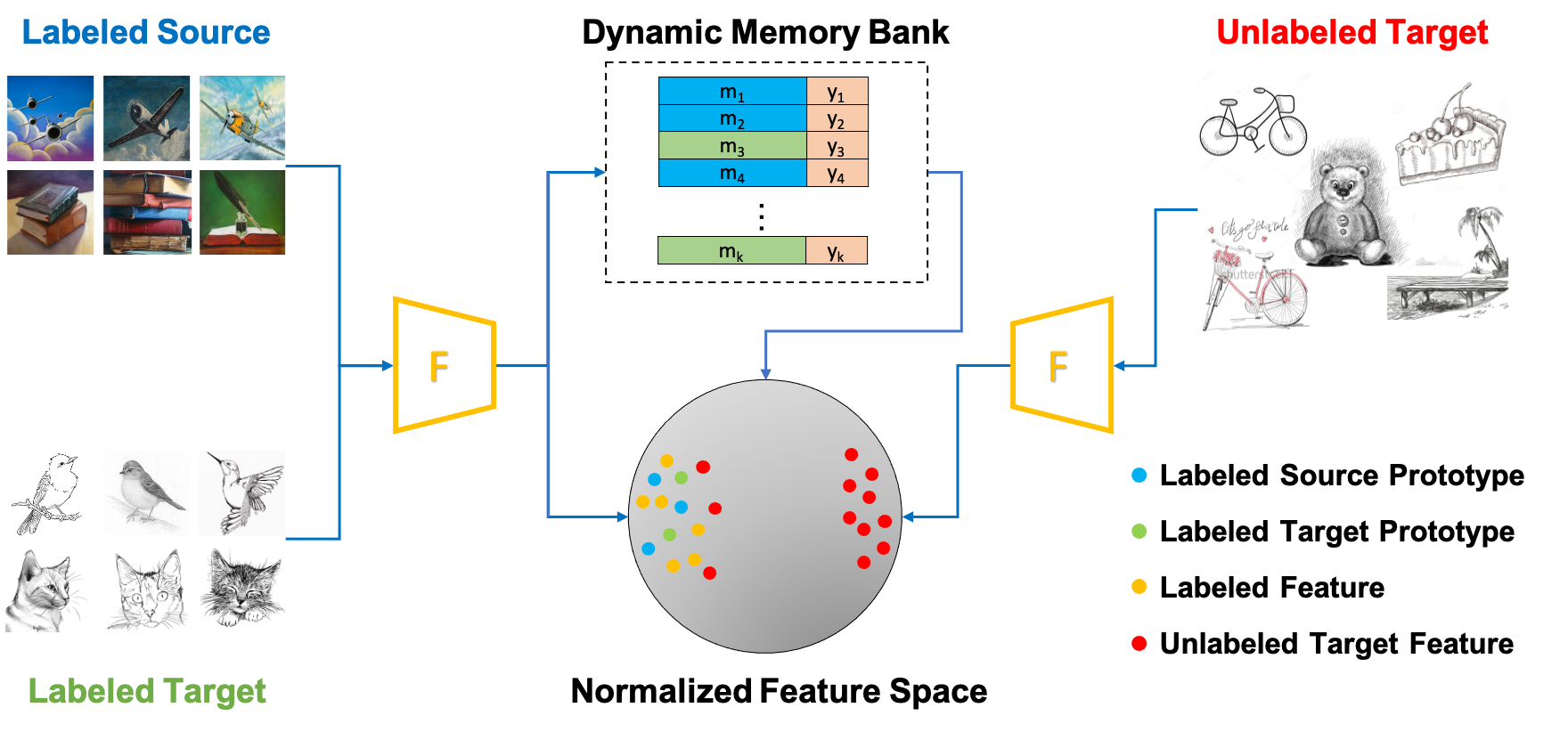
Figure 1: Framework of Dynamic Feature Alignment. Both labeled source and labeled target samples are passed into the feature extractor $F$. Normalized feature embeddings and labels are then stored in the dynamic memory bank as class prototypes for dynamic alignment and pseudo-labeling. The feature extractor for unlabeled target samples shares the same weights.

3.2 Supervised Classification in Normalized Feature Space

Our proposed DFA framework aligns the features of labeled examples from both domains using a supervised classification loss. A feature extractor $f(\cdot)$ is trained to extract the features from the input image ${x}$. The feature $m$, which is normalized to be unit length, is represented as:

$$m=f(x).$$ (1)

The classifier takes as inputs the normalized features $m$ and compares the cosine similarity between $m$ and the prototype weight vector $\mathbf{w}_{k}$ ($k$ = 1, …, K) of class $k$. The similarities are scaled by a temperature $\tau=0.05$, which controls the concentration level of the distribution [Hinton et al.(2015)Hinton, Vinyals, and Dean, Wang et al.(2017)Wang, Xiang, Cheng, and Yuille]. The probability of $m$ being categorized as class $k$ can be presented as:

$$P(k|m)=\frac{exp(\mathbf{w}^{T}\cdot m/\tau)}{\sum_{j=1}^{K}exp(\mathbf{w}^{T}_{j}\cdot m/\tau)}.$$ (2)

$P(k|m)$ is then passed to the classification loss [Wu et al.()Wu, Xiong, Yu, and Lin, He et al.()He, Fan, Wu, Xie, and Girshick]. During training, we utilize cross-entropy as the supervised classification loss:

$$\mathcal{L}_{cls}=-\mathbb{E}_{(\mathbf{x},y)\in\mathcal{D}_{s}\cup\mathcal{D}_{l}}\sum_{k=1}^{K}\log P_{k}.$$ (3)

When aligning the normalized features by training the network, the labeled target features $f(x^{l})$ are closely aligned to the labeled source features $f(x^{s})$ [Saito et al.()Saito, Kim, Sclaroff, Darrell, and Saenko, Kim and Kim()], and we aim to utilize both labeled source and target samples and reduce the domain shift.

3.3 Dynamic Memory Bank

We propose to maintain a dynamic memory bank $\mathcal{B}$ that stores representative features, which we call prototypes, for each class. If our feature extractor was fixed, we could simply extract all the features once and compute their averages. This isn’t feasible since we are actively updating our feature extractor. We could recompute the prototypes periodically, but this would be computationally expensive. Instead we keep a weighted average of recently extracted features. A natural strategy for maintaining the memory bank would be to update the corresponding class prototype for each labeled sample in the current mini-batch. This could be done, for example, as an exponentially weighted moving average (EWMA). The downside of this approach is that the class prototype for common classes would update more frequently, which leads to difficulty in setting update weights. It also doesn’t take into account the potential for a large domain shift to lead to less informative class prototypes, especially when many samples are misclassified.

To maintain our dynamic memory bank $\mathcal{B}$, we propose to use an intermediate memory bank $b$ to enable us to make consistent, class-balanced updates. For every minibatch, we update $b$ as follows: we check the network output $f(x_{k})$ on the input image $x_{k}$, which could be from the source or target domain. If $x_{k}$ is correctly classified, then the corresponding vector in $b$ is replaced with $f(x_{k})$. Therefore, $b$ always stores the feature of the most recent correctly classified image for each class. We use the intermediate memory bank $b$ to update $\mathcal{B}$, using an EWMA, as follows:

$$\mathcal{B}=\gamma\cdot\mathcal{B}_{t-1}+(1-\gamma)\cdot b$$ (4)

where $\gamma$ regulates the pace of the update: lower value results in a faster updating pace, and higher value leads to a slower update.

The dynamic memory bank $\mathcal{B}$ is updated based on labeled source features $f(x^{s})$ and labeled target features $f(x^{l})$. Therefore, each feature vector in $\mathcal{B}$ represents a class, and can be interpreted as a class prototype, so $\mathcal{B}$ stores the prototypes of all classes. In the following section, we describe how this dynamic memory bank can be applied to (1) align the unlabeled target features to class prototypes accurately and (2) selectively collect unlabeled samples for pseudo-label estimation.

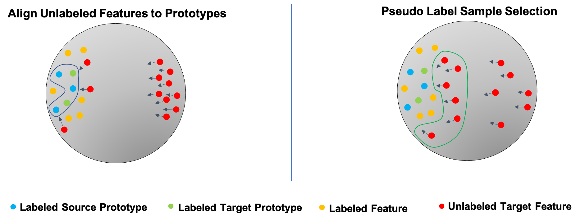
Figure 2: Illustration of Dynamic Feature Alignment. (left) Shows that unlabeled target features (red dots) gradually move to class prototypes of the source (blue dots) and target (green dots). (right) Shows that unlabeled target features with lower entropy values and higher similarity scores (surrounded by the green curve) will be selected for pseudo-label training.

3.4 Dynamic Feature Alignment

Since the labeled target features $f(x^{l})$ are already closely aligned to the labeled source features $f(x^{s})$ [Saito et al.()Saito, Kim, Sclaroff, Darrell, and Saenko, Kim and Kim()], we focus on the intra-domain discrepancy by directly minimizing the distance between $f(x^{u})$ and class prototypes. We choose to use Maximum Mean Discrepancy (MMD) [Gretton et al.()Gretton, Borgwardt, Rasch, Schölkopf, and Smola] to measure the difference between distributions. The basic idea of MMD is that if two distributions are identical, then all the statistics of these two should be the same [Zhu et al.()Zhu, Zhuang, and Wang].

$$D_{\mathcal{H}}(\mathcal{B},\mathcal{D}_{u})\triangleq\left\|\mathbb{E}_{\mathcal{B}}[\phi(m_{i})]-\mathbb{E}_{\mathcal{D}_{u}}[\phi(f(x_{j}^{u}))]\right\|_{\mathcal{H}}^{2},$$ (5)

where $m_{i}$ is the $i$-th feature stored in $\mathcal{B}$, representing the prototype of class $i$, and $f(x_{j}^{u})$ is the $j$-th feature in the unlabeled target features $\mathcal{D}_{u}$. Here $\phi(\cdot)$ represents Gaussian Radial Basis Function (RBF) kernels, which map the input feature maps to the reproducing kernel Hilbert space $\mathcal{H}$. The MMD loss can be presented as:

$$\mathcal{L}_{mmd}=D_{\mathcal{H}}(\mathcal{B},\mathcal{D}_{u}).$$ (6)

By minimizing $\mathcal{L}_{mmd}$, the domain discrepancy will be bridged and unaligned target features are gradually moving close to the aligned class prototypes. See Fig 2 (left) for illustration.

To accelerate the learning process as well as further improve the accuracy, we take advantage of the large number of unlabeled samples and propose a pseudo-label estimation strategy. For an unlabeled image $x^{u}$, we compute the distances between $f(x^{u})$ and every class prototype $m$ stored in $\mathcal{B}$. Here, the cosine similarity is used for distance measurement. Since $m_{i}$ is the representative prototype of the $i$-th class, a higher similarity value represents a higher probability that $x^{u}$ belongs to class $i$. Then the pseudo-label estimation function can be formulated by using a softmax function with a temperature $\tau_{p}$ as follows:

$$P_{dist}(i|x^{u})=\frac{exp(m^{T}\cdot f(x^{u})/\tau_{p})}{\sum_{j=1}^{K}exp(m^{T}_{j}\cdot f(x^{u})/\tau_{p})}.$$ (7)

Training with inaccurate pseudo-labels can accumulate errors. We adopt a sample selection strategy to keep the high-quality pseudo-labels in the training loop and eliminate the inaccurate ones. First, those samples with similarity scores higher than the threshold $\epsilon_{dist}$ will be stored in $M_{dist}$. Second, we collect samples with the prediction entropy $H_{\mathbf{w}}(P_{dist})$ less than a threshold $\epsilon_{ent}$ and store them in $M_{ent}$. This step will selectively collect the samples that are close to the aligned features [Kim and Kim()]. See Fig 2 (right) for illustration. Last, we take the intersection of $M_{dist}$ and $M_{ent}$, noted as $M_{pse}$. Thus, only samples satisfying both conditions will be used in the pseudo-label training loop.

The network output $\hat{y}_{x}$ of each sample $x$ in $M_{pse}$ is used as the pseudo-label for calculating the cross entropy loss $\mathcal{L}_{pseudo}$:

$$\mathcal{L}_{pseudo}=-\mathbb{E}_{\mathcal{D}_{u}}[\mathbf{1}_{M_{pse}}(x)\log p(y=\hat{y}_{x}|x)].$$ (8)

To further minimize the intra-domain discrepancy, we follow [Kim and Kim()] and apply the same perturbation scheme. We regularize the perturbed features and the raw, clean features by Kullback–Leibler divergence. The goal is to enforce the model to generate perturbation-invariant features so that the perturbation loss can be presented as:

$$\mathcal{L}_{perturb}=\mathbb{E}_{\mathbf{x}\in\mathcal{D}_{u}\cup\mathcal{D}_{l}}\bigg{[}\sum_{i=1}^{K}KL[f(x),f(x+r_{x})]\bigg{]},$$ (9)

where $x$ is the input image, and $r_{x}$ is the optimized perturbation added to $x$.

3.5 Overall Loss Function

The overall loss function of the proposed DFA framework is the weighted sum of every different piece of loss function mentioned above and can be integrated as follows:

$$\mathcal{L}=\mathcal{L}_{cls}+\alpha_{1}\mathcal{L}_{mmd}+\alpha_{2}\mathcal{L}_{pseudo}+\alpha_{3}\mathcal{L}_{perturb}.$$ (10)

4 Experiments

We evaluate our method by conducting experiments on two standard domain adaptation benchmarks. Below we describe the datasets used for these experiments, implementation details, and extensive performance analysis.

4.1 Datasets

DomainNet [Peng et al.()Peng, Bai, Xia, Huang, Saenko, and Wang] is a large-scale domain adaptation benchmark that contains 6 domains and 345 object categories. Following the previous works MME [Saito et al.()Saito, Kim, Sclaroff, Darrell, and Saenko] and APE [Kim and Kim()], we use a 4 domain (Real, Clipart, Painting, Sketch) subset with 126 classes. We report our results on 7 scenarios for a fair comparison with the previous state-of-the-art works.

We also evaluate our model on Office-Home [Venkateswara et al.()Venkateswara, Eusebio, Chakraborty, and Panchanathan], which is another domain adaptation benchmark that contains 4 domains (Real, Clipart, Art, Product) and 65 categories. Here we report results on all 12 adaptation scenarios.

4.2 Implementation Details

We implement our model using PyTorch [Paszke et al.(2019)Paszke, Gross, Massa, Lerer, Bradbury, Chanan, Killeen, Lin, Gimelshein, Antiga, et al.]. We follow [Saito et al.()Saito, Kim, Sclaroff, Darrell, and Saenko, Kim and Kim()] and report results on DomainNet using AlexNet and ResNet-34 as the backbones. For Office-Home, we report on ResNet-34. All networks are pre-trained on ImageNet. Our model is trained on labeled $\mathcal{D}_{s}$, $\mathcal{D}_{l}$, and unlabeled $\mathcal{D}_{u}$. To make the source and target balanced in the training stage, each mini-batch of labeled samples contains half source samples and half target samples. We consider both one-shot and three-shot setting, and for each class, one (or three) labeled target samples are given for training. For evaluation, we reveal the ground-truth labels of $\mathcal{D}_{u}$ and report results on that. We follow [Saito et al.()Saito, Kim, Sclaroff, Darrell, and Saenko, Kim and Kim()] and use SGD optimizer with an initial learning rate of 0.01, a momentum of 0.9, and a weight decay of 0.0005. For hyperparameters, we set the temperature for the classifier as $\tau=0.05$, set $\gamma=0.1$ to update $\mathcal{B}$ in a fast pace. We set the temperature for pseudo-label estimation as $\tau_{p}=0.07$. As for thresholds, we set $\epsilon_{dist}$ to $0.3$ for ResNet-34 and $0.1$ for AlexNet, and set $\epsilon_{ent}=0.5$ for both backbone networks.

4.3 Baselines

We compare our proposed method with different models. Baselines include training a network only using labeled samples (S+T), a entropy minimization based semi-supervised method (ENT [Grandvalet et al.(2005)Grandvalet, Bengio, et al.]), three feature alignment-based unsupervised domain adaptation models (DANN [Ganin and Lempitsky()], ADR [Saito et al.(2017)Saito, Ushiku, Harada, and Saenko], and CDAN [Long et al.(2017)Long, Cao, Wang, and Jordan]), and three state-of-the-art semi-supervised learning models (SagNet [Nam et al.()Nam, Lee, Park, Yoon, and Yoo], MME [Saito et al.()Saito, Kim, Sclaroff, Darrell, and Saenko], and APE [Kim and Kim()]) that aim to the same goal as our method.

Table 1: Classification accuracy (%) on the DomainNet dataset for three-shot setting with 4 domains, 7 scenarios using AlexNet and ResNet-34 as backbone networks, respectively.

Net	Method	R to C	R to P	P to C	C to S	S to P	R to S	P to R	MEAN
AlexNet	S+T	47.1	45.0	44.9	36.4	38.4	33.3	58.7	43.4
	DANN	46.1	43.8	41.0	36.5	38.9	33.4	57.3	42.4
	ADR	46.2	44.4	43.6	36.4	38.9	32.4	57.3	42.7
	CDAN	46.8	45.0	42.3	29.5	33.7	31.3	58.7	41.0
	ENT	45.5	42.6	40.4	31.1	29.6	29.6	60.0	39.8
	MME	55.6	49.0	51.7	39.4	43.0	37.9	60.7	48.2
	SagNet	49.1	46.7	46.3	39.4	39.8	37.5	57.0	45.1
	APE	54.6	50.5	52.1	42.6	42.2	38.7	61.4	48.9
	Ours	55.0	52.3	51.6	44.5	41.8	39.4	62.1	49.5
ResNet	S+T	60.0	62.2	59.4	55.0	59.5	50.1	73.9	60.0
	DANN	59.8	62.8	59.6	55.4	59.9	54.9	72.2	60.7
	ADR	60.7	61.9	60.7	54.4	59.9	51.1	74.2	60.4
	CDAN	69.0	67.3	68.4	57.8	65.3	59.0	78.5	66.5
	ENT	71.0	69.2	71.1	60.0	62.1	61.1	78.6	67.6
	MME	72.2	69.7	71.7	61.8	66.8	61.9	78.5	68.9
	SagNet	62.0	62.9	61.5	57.1	59.0	54.4	73.4	61.5
	APE	76.6	72.1	76.7	63.1	66.1	67.5	79.4	71.7
	Ours	76.7	73.9	75.4	65.5	70.5	67.5	80.3	72.8

Table 2: Classification accuracy (%) on the DomainNet dataset for one-shot setting with 4 domains, 7 scenarios using ResNet-34.

Net	Method	R to C	R to P	P to C	C to S	S to P	R to S	P to R	MEAN
ResNet	S+T	55.6	60.6	56.8	50.8	56.0	46.3	71.8	56.9
	DANN	58.2	61.4	56.3	52.8	57.4	52.2	70.3	58.4
	ADR	57.1	61.3	57.0	51.0	56.0	49.0	72.0	57.6
	CDAN	65.0	64.9	63.7	53.1	63.4	54.5	73.2	62.5
	ENT	65.2	65.9	65.4	54.6	59.7	52.1	75.0	62.6
	MME	70.0	67.7	69.0	56.3	64.8	61.0	76.1	66.4
	SagNet	59.4	61.9	59.1	54.0	56.6	49.7	72.2	59.0
	APE	70.4	70.8	72.9	56.7	64.5	63.0	76.6	67.6
	Ours	71.8	72.7	69.8	60.8	68.0	62.3	76.8	68.9

Table 3: Classification accuracy (%) comparisons on Office-Home for three-shot setting with 4 domains, 12 scenarios using ResNet-34 as the backbone network.

Method	R to C	R to P	R to A	P to R	P to C	P to A	A to P	A to C	A to R	C to R	C to A	C to P	MEAN
S+T	55.7	80.8	67.8	73.1	53.8	63.5	73.1	54.0	74.2	68.3	57.6	72.3	66.2
DANN	57.3	75.5	65.2	69.2	51.8	56.6	68.3	54.7	73.8	67.1	55.1	67.5	63.5
CDAN	61.4	80.7	67.1	76.8	58.1	61.4	74.1	59.2	74.1	70.7	60.5	74.5	68.2
ENT	62.6	85.7	70.2	79.9	60.5	63.9	79.5	62.3	79.1	76.4	64.7	79.1	71.9
MME	64.6	85.5	71.3	80.1	64.6	65.5	79.0	63.6	79.7	76.6	67.2	79.3	73.1
APE	66.4	86.2	73.4	82.0	65.2	66.1	81.1	63.9	80.2	76.8	66.6	79.9	74.0
Ours	68.3	86.9	74.1	82.3	65.9	67.8	80.4	63.0	80.3	76.6	67.8	79.1	74.4

4.4 Experiment Results

We summarize the comparisons between our method and the baselines on 7 adaptation scenarios of the DomainNet dataset in Table 1 and Table 2, for three-shot setting and one-shot setting respectively. When using the ResNet-34 as the backbone network, our method outperforms the current state-of-the-art baseline by more than $1\%$, and achieves the best performance in most adaptation scenarios. For the best case S to P of three-shot setting, our method surpasses the second-best method by $4.4\%$. When AlexNet is applied as the backbone network, the margin that our method outperforms other methods is not as large as using ResNet-34 because our proposed scheme requires high-quality intermediate features stored in $\mathcal{B}$, and ResNet-34 has more advantage in achieving that compared with AlexNet. Our method still performs the best in most scenarios, surpassing APE by $0.6\%$ on average.

The comparison results of our method with other baselines of 12 adaptation scenarios on Office-Home dataset are summarized in Table 3. We report results using ResNet-34 as the backbone network. Our method achieves the best performance on 8 out of 12 adaptation scenarios and outperforms all the baselines on average.

4.5 Analysis

In Sec 3.3, we explain the updating rules of the dynamic memory bank $\mathcal{B}$. Here we conduct an experiment to show how $\gamma$ affects the classification accuracy. We use AlexNet as the backbone network and train the model on DomainNet with different $\gamma$. A smaller $\gamma$ means updating $\mathcal{B}$ faster, and larger $\gamma$ means updating $\mathcal{B}$ in a more stable way. We evaluate on 3 adaptation scenarios and summarize the results in Table 4. It demonstrates that a more stable $\mathcal{B}$ (with larger $\gamma$ as 0.75) can not help improve the performance, and replacing the entire $\mathcal{B}$ with the new one every iteration ($\gamma=0$) can not get the optimal performance either. Our results show that using a small (but larger than $0$) $\gamma$ and updating $\mathcal{B}$ in a relatively faster pace achieves the best classification accuracy.

Table 4: Analysis on how $\gamma$ affects the classification accuracy ($\%$).

Method	R to C	R to P	C to S	MEAN
APE	54.6	50.5	42.6	49.2
Ours ($\gamma=0.75$)	54.1	50.7	42.4	49.0
Ours ($\gamma=0.25$)	54.9	52.2	43.6	50.2
Ours ($\gamma=0.1$)	55.0	52.3	44.5	50.6
Ours ($\gamma=0$)	54.7	52.0	44.5	50.4

To better understand the feature alignment progress, we show the t-SNE [Van der Maaten and Hinton()] embedding of the intermediate features at different training stages in Fig 3. We visualize the target features extracted by ResNet-34 in the experiment of Painting to Real scenario of the DomainNet. Following APE [Kim and Kim()], we randomly select 20 classes out of 126 classes in the dataset for clarity. This shows that as training progresses, the target feature clusters will gradually be split for better classification.

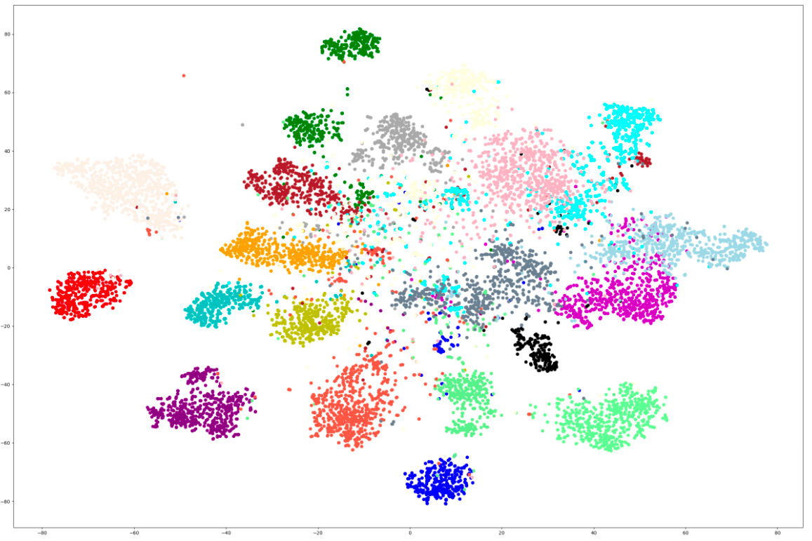
Epoch 1	Epoch 10
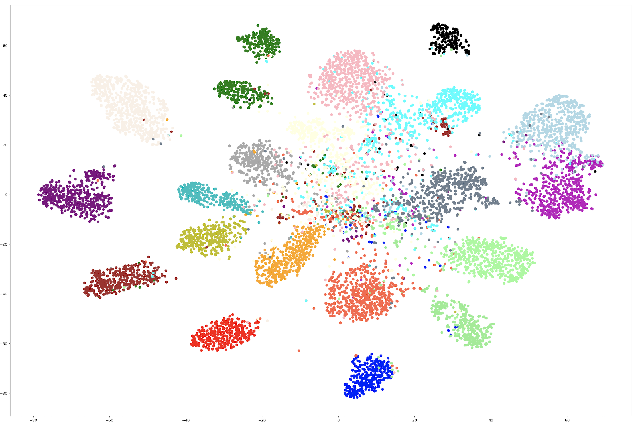
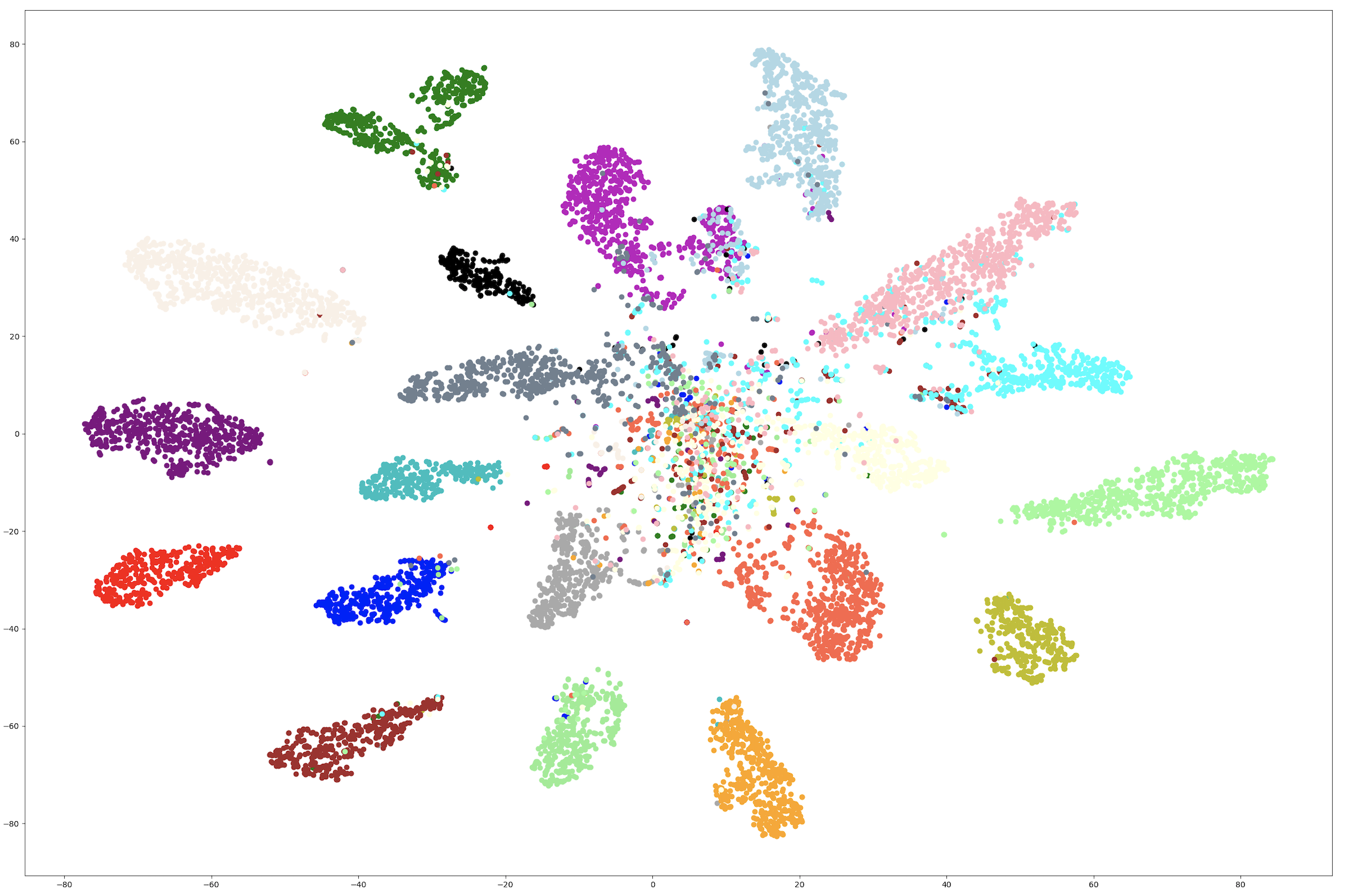
Epoch 50	Epoch 100

Figure 3: The t-SNE visualization of intermediate features in the target domain of our method at different training stages.

5 Conclusions

We proposed a novel approach for semi-supervised domain adaptation that uses a dynamic memory bank to support inter- and intra-domain feature alignment. Our update approach is designed to be class balanced, thereby mitigating one of the more challenging aspects of the problem. We evaluated our approach on two standard datasets and found that it significantly improved the average accuracy over the previous state-of-the-art techniques. In addition to improved accuracy, our approach has several attractive features. It doesn’t require significant additional memory (only two copies of the class prototypes) or computation (only online updates to the intermediate and dynamic memory banks). It also doesn’t require extensive parameter tuning: the weights for the loss function are fixed across all experiments, accuracy isn’t particularly sensitive to the dynamic memory updates parameter $\gamma$, and the pseudo-label thresholds only needed to be adjusted to account for the low discriminative power of AlexNet. Given this, we believe this approach will be applicable to many semi-supervised domain adaptation scenarios.

Acknowledgements

This material is based upon work supported by the National Science Foundation under Grant No. IIS-1553116.

References

- [Ao et al.()Ao, Li, and Ling] Shuang Ao, Xiang Li, and Charles X Ling. Fast generalized distillation for semi-supervised domain adaptation. In AAAI 2017.
- [Ben-David et al.(2010)Ben-David, Blitzer, Crammer, Kulesza, Pereira, and Vaughan] Shai Ben-David, John Blitzer, Koby Crammer, Alex Kulesza, Fernando Pereira, and Jennifer Wortman Vaughan. A theory of learning from different domains. Machine learning, 2010.
- [Bousmalis et al.()Bousmalis, Trigeorgis, Silberman, Krishnan, and Erhan] Konstantinos Bousmalis, George Trigeorgis, Nathan Silberman, Dilip Krishnan, and Dumitru Erhan. Domain separation networks. NeurIPS 2016.
- [Cao et al.()Cao, Long, and Wang] Yue Cao, Mingsheng Long, and Jianmin Wang. Unsupervised domain adaptation with distribution matching machines. In AAAI 2018.
- [Donahue et al.()Donahue, Hoffman, Rodner, Saenko, and Darrell] Jeff Donahue, Judy Hoffman, Erik Rodner, Kate Saenko, and Trevor Darrell. Semi-supervised domain adaptation with instance constraints. In CVPR 2013.
- [Dong et al.()Dong, Cong, Sun, Liu, and Xu] Jiahua Dong, Yang Cong, Gan Sun, Yuyang Liu, and Xiaowei Xu. Cscl: Critical semantic-consistent learning for unsupervised domain adaptation. In ECCV 2020.
- [Dong et al.(2020)Dong, Cong, Sun, Zhong, and Xu] Jiahua Dong, Yang Cong, Gan Sun, Bineng Zhong, and Xiaowei Xu. What can be transferred: Unsupervised domain adaptation for endoscopic lesions segmentation. In CVPR, 2020.
- [Ganin and Lempitsky()] Yaroslav Ganin and Victor Lempitsky. Unsupervised domain adaptation by backpropagation. In ICML 2015.
- [Ganin et al.()Ganin, Ustinova, Ajakan, Germain, Larochelle, Laviolette, Marchand, and Lempitsky] Yaroslav Ganin, Evgeniya Ustinova, Hana Ajakan, Pascal Germain, Hugo Larochelle, François Laviolette, Mario Marchand, and Victor Lempitsky. Domain-adversarial training of neural networks. JMLR 2016.
- [Ghifary et al.()Ghifary, Kleijn, Zhang, and Balduzzi] Muhammad Ghifary, W Bastiaan Kleijn, Mengjie Zhang, and David Balduzzi. Domain generalization for object recognition with multi-task autoencoders. In ICCV 2015.
- [Ghifary et al.(2016)Ghifary, Kleijn, Zhang, Balduzzi, and Li] Muhammad Ghifary, W Bastiaan Kleijn, Mengjie Zhang, David Balduzzi, and Wen Li. Deep reconstruction-classification networks for unsupervised domain adaptation. In ECCV, 2016.
- [Grandvalet et al.(2005)Grandvalet, Bengio, et al.] Yves Grandvalet, Yoshua Bengio, et al. Semi-supervised learning by entropy minimization. In CAP, pages 281–296, 2005.
- [Gretton et al.()Gretton, Borgwardt, Rasch, Schölkopf, and Smola] Arthur Gretton, Karsten M Borgwardt, Malte J Rasch, Bernhard Schölkopf, and Alexander Smola. A kernel two-sample test. JMLR 2012.
- [Gretton et al.(2006)Gretton, Borgwardt, Rasch, Schölkopf, and Smola] Arthur Gretton, Karsten Borgwardt, Malte Rasch, Bernhard Schölkopf, and Alex Smola. A kernel method for the two-sample-problem. NeurIPS, 2006.
- [He et al.()He, Fan, Wu, Xie, and Girshick] Kaiming He, Haoqi Fan, Yuxin Wu, Saining Xie, and Ross Girshick. Momentum contrast for unsupervised visual representation learning. In CVPR 2020.
- [Hinton et al.(2015)Hinton, Vinyals, and Dean] Geoffrey Hinton, Oriol Vinyals, and Jeff Dean. Distilling the knowledge in a neural network. arXiv preprint arXiv:1503.02531, 2015.
- [Hoffman et al.()Hoffman, Tzeng, Park, Zhu, Isola, Saenko, Efros, and Darrell] Judy Hoffman, Eric Tzeng, Taesung Park, Jun-Yan Zhu, Phillip Isola, Kate Saenko, Alexei Efros, and Trevor Darrell. Cycada: Cycle-consistent adversarial domain adaptation. In ICML 2018.
- [Jiang et al.()Jiang, Wu, Han, Shao, Qi, and Li] Pin Jiang, Aming Wu, Yahong Han, Yunfeng Shao, Meiyu Qi, and Bingshuai Li. Bidirectional adversarial training for semi-supervised domain adaptation. IJCAI 2020.
- [Kang et al.()Kang, Jiang, Yang, and Hauptmann] Guoliang Kang, Lu Jiang, Yi Yang, and Alexander G Hauptmann. Contrastive adaptation network for unsupervised domain adaptation. In CVPR 2019.
- [Kim and Kim()] Taekyung Kim and Changick Kim. Attract, perturb, and explore: Learning a feature alignment network for semi-supervised domain adaptation. In ECCV 2020.
- [Liu and Tuzel(2016)] Ming-Yu Liu and Oncel Tuzel. Coupled generative adversarial networks. In NeurIPS, 2016.
- [Liu and Mukhopadhyay(2018)] Qun Liu and Supratik Mukhopadhyay. Unsupervised learning using pretrained cnn and associative memory bank. In IJCNN. IEEE, 2018.
- [Long et al.(2017)Long, Cao, Wang, and Jordan] Mingsheng Long, Zhangjie Cao, Jianmin Wang, and Michael I Jordan. Conditional adversarial domain adaptation. arXiv preprint arXiv:1705.10667, 2017.
- [Motiian et al.(2017)Motiian, Jones, Iranmanesh, and Doretto] Saeid Motiian, Quinn Jones, Seyed Mehdi Iranmanesh, and Gianfranco Doretto. Few-shot adversarial domain adaptation. arXiv preprint arXiv:1711.02536, 2017.
- [Nam et al.()Nam, Lee, Park, Yoon, and Yoo] Hyeonseob Nam, HyunJae Lee, Jongchan Park, Wonjun Yoon, and Donggeun Yoo. Reducing domain gap by reducing style bias. In CVPR 2021.
- [Paszke et al.(2019)Paszke, Gross, Massa, Lerer, Bradbury, Chanan, Killeen, Lin, Gimelshein, Antiga, et al.] Adam Paszke, Sam Gross, Francisco Massa, Adam Lerer, James Bradbury, Gregory Chanan, Trevor Killeen, Zeming Lin, Natalia Gimelshein, Luca Antiga, et al. Pytorch: An imperative style, high-performance deep learning library. arXiv preprint arXiv:1912.01703, 2019.
- [Peng et al.()Peng, Bai, Xia, Huang, Saenko, and Wang] Xingchao Peng, Qinxun Bai, Xide Xia, Zijun Huang, Kate Saenko, and Bo Wang. Moment matching for multi-source domain adaptation. In CVPR 2019.
- [Redko et al.(2019)Redko, Morvant, Habrard, Sebban, and Bennani] Ievgen Redko, Emilie Morvant, Amaury Habrard, Marc Sebban, and Younes Bennani. Advances in domain adaptation theory. Elsevier, 2019.
- [Rozantsev et al.(2018)Rozantsev, Salzmann, and Fua] Artem Rozantsev, Mathieu Salzmann, and Pascal Fua. Beyond sharing weights for deep domain adaptation. TPAMI, 2018.
- [Saito et al.()Saito, Kim, Sclaroff, Darrell, and Saenko] Kuniaki Saito, Donghyun Kim, Stan Sclaroff, Trevor Darrell, and Kate Saenko. Semi-supervised domain adaptation via minimax entropy. In CVPR 2019.
- [Saito et al.(2017)Saito, Ushiku, Harada, and Saenko] Kuniaki Saito, Yoshitaka Ushiku, Tatsuya Harada, and Kate Saenko. Adversarial dropout regularization. arXiv preprint arXiv:1711.01575, 2017.
- [Sun and Saenko()] Baochen Sun and Kate Saenko. Deep coral: Correlation alignment for deep domain adaptation. In ECCV 2016.
- [Sun et al.()Sun, Feng, and Saenko] Baochen Sun, Jiashi Feng, and Kate Saenko. Return of frustratingly easy domain adaptation. In AAAI 2016.
- [Teshima et al.()Teshima, Sato, and Sugiyama] Takeshi Teshima, Issei Sato, and Masashi Sugiyama. Few-shot domain adaptation by causal mechanism transfer. In ICML 2020.
- [Van der Maaten and Hinton()] Laurens Van der Maaten and Geoffrey Hinton. Visualizing data using t-sne. JMLR 2008.
- [Venkateswara et al.()Venkateswara, Eusebio, Chakraborty, and Panchanathan] Hemanth Venkateswara, Jose Eusebio, Shayok Chakraborty, and Sethuraman Panchanathan. Deep hashing network for unsupervised domain adaptation. In CVPR 2017.
- [Wang et al.(2017)Wang, Xiang, Cheng, and Yuille] Feng Wang, Xiang Xiang, Jian Cheng, and Alan Loddon Yuille. Normface: L2 hypersphere embedding for face verification. In Proceedings of the 25th ACM international conference on Multimedia, 2017.
- [Wang and Deng(2018)] Mei Wang and Weihong Deng. Deep visual domain adaptation: A survey. Neurocomputing, 2018.
- [Wilson and Cook(2020)] Garrett Wilson and Diane J Cook. A survey of unsupervised deep domain adaptation. ACM Transactions on Intelligent Systems and Technology (TIST), 2020.
- [Wu et al.()Wu, Xiong, Yu, and Lin] Zhirong Wu, Yuanjun Xiong, Stella X Yu, and Dahua Lin. Unsupervised feature learning via non-parametric instance discrimination. In CVPR 2018.
- [Yao et al.()Yao, Pan, Ngo, Li, and Mei] Ting Yao, Yingwei Pan, Chong-Wah Ngo, Houqiang Li, and Tao Mei. Semi-supervised domain adaptation with subspace learning for visual recognition. In CVPR 2015.
- [Zhu et al.(2017)Zhu, Park, Isola, and Efros] Jun-Yan Zhu, Taesung Park, Phillip Isola, and Alexei A Efros. Unpaired image-to-image translation using cycle-consistent adversarial networks. In ICCV, 2017.
- [Zhu et al.()Zhu, Zhuang, and Wang] Yongchun Zhu, Fuzhen Zhuang, and Deqing Wang. Aligning domain-specific distribution and classifier for cross-domain classification from multiple sources. In AAAI 2019.