Complexity of Scalar Collapse in Anti-de Sitter Spacetime

Abstract

We calculate the volume and action forms of holographic complexity for the gravitational collapse of scalar field matter in asymptotically anti-de Sitter spacetime, using numerical methods to reproduce the geometry responding to the oscillating field over multiple crossing times. Like the scalar field pulse, the volume complexity oscillates quasiperiodically before horizon formation. It also shows a scaling symmetry with the amplitude of the scalar field. The action complexity is also quasiperiodic with spikes of increasing amplitude.

1 Introduction

Recent years have seen a rapid growth of interest in (circuit) complexity as an information theoretic quantity of relevance to fundamental physics, following the foundational work of arXiv:1402.5674 ; arXiv:1406.2678 ; arXiv:1509.07876 ; arXiv:1512.04993 . In quantum mechanics and quantum field theory, complexity is a measure of distance of the state in question from a reference state quant-ph/0502070 ; quant-ph/0603161 ; quant-ph/0701004 ; arXiv:1707.08570 ; arXiv:1801.07620 ; arXiv:1803.10638 representing the minimal amount of computational processing needed to generate that state (i.e., the size of the optimal circuit required in a quantum computer using a specified set of basis gates). Therefore, like entropy represents the information content of a system, the time derivative of complexity represents processing speed.

Also like entropy, the complexity of states in field theories with gravity duals should have a holographic interpretation in terms of geometry. In the AdS/CFT correspondence, there are in fact two proposals for a holographic definition of complexity for the state on a spacelike slice $\Sigma$ of the conformal boundary of anti-de Sitter spacetime (AdS). The first is “$\mathcal{C}=V$” complexity arXiv:1402.5674 ; arXiv:1406.2678 , which assigns the complexity as $\mathcal{C}_{V}=\max[V(\mathcal{B})/G\ell]$, where the maximum is over spacelike bulk surfaces $\mathcal{B}$ with boundary on $\Sigma$, $G$ is the Newton constant of the AdS spacetime, and $\ell$ is some length scale depending on the asymptotically AdS geometry (typically either the AdS curvature scale or the Schwarzschild radius of a small black hole). The other proposal, “$\mathcal{C}=A$,” states that the complexity of the state on $\Sigma$ is $\mathcal{C}_{A}=S_{WDW}/\pi$ (in units with $\hbar=1$), where $S_{WDW}$ is the action of the Wheeler–DeWitt (WDW) patch of $\Sigma$ in the bulk arXiv:1509.07876 ; arXiv:1512.04993 . The WDW patch is the union of spacelike bulk surfaces with boundary on $\Sigma$, so the WDW patch is bounded by past- and future-directed lightlike surfaces emitted from $\Sigma$ into the bulk. $S_{WDW}$ includes boundary terms as well as joint terms on $\Sigma$.

In both proposals, the complexity of eternal AdS black holes exhibits linear growth in time, as expected for a thermal equilibrium state (see arXiv:1406.2678 ; arXiv:1509.07876 for the initial calculations). Of course, the contribution of time evolution of the spacetime background to time dependence of complexity is an important question; arXiv:1408.2823 ; arXiv:1711.02668 ; arXiv:1802.06740 ; arXiv:1803.11162 ; arXiv:1804.07410 ; Lezgi:2021qog have studied complexity in black hole formation due to the collapse of a thin shell of null matter (i.e., the AdS-Vaidya geometry) as a probe both of complexity during thermalization of the dual CFT and of both proposals for holographic complexity. As summarized in arXiv:1804.07410 , the complexity of the collapsing geometry approaches the linear growth rate of eternal black holes at late times following transient behavior in the early stages of the shell’s collapse.

Our purpose is to examine the transient early time behavior of complexity for the collapse of a smooth distribution of matter rather than a thin shell. There is a critical difference between these two cases in asymptotically AdS spacetime with the conformal boundary $\mathbb{R}\times S^{d-1}$ of AdS in global coordinates (henceforth, “asymptotically global AdS”): while thin shells always form an apparent horizon promptly, a smooth distribution of matter may collapse, disperse, reflect from the conformal boundary, and collapse again many times before finally forming a horizon, as argued initially for massless scalars with spherical symmetry in arXiv:1104.3702 ; arXiv:1106.2339 ; arXiv:1108.4539 ; arXiv:1110.5823 . For a fixed profile of initial data for the scalar field, lower initial amplitudes take a longer time to form a black hole, but instability to eventual horizon formation seems to be generic; however, there is a so-called “island of stability” for initial profiles with characteristic width near the AdS scale with quasiperiodic scalar and gravitational evolution arXiv:1304.4166 ; arXiv:1307.2875 ; arXiv:1308.1235 ; Evnin:2021buq . Because unstable initial data also evolves quasiperiodically prior to horizon formation, determining whether a given set of initial data is stable or unstable at low amplitudes is a topic of interest in the literature. While massless scalars are better studied, massive scalars exhibit similar behavior arXiv:1504.05203 ; arXiv:1508.02709 ; arXiv:1711.00454 .

As a step toward understanding complexity in time-dependent asymptotically global AdS spacetimes with smooth matter distributions, we calculate volume and action complexity at early times in the gravitational collapse of spherically symmetric scalar fields. One question of interest is whether complexity evolves quasiperiodically or if it demonstrates a trend over oscillations of the scalar field packet, which we will refer to as “ratcheting” behavior. We might expect ratcheting as an indication that the scalar field undergoes gravitational focusing throughout its oscillation, which eventually leads to horizon formation.

We begin with a review of scalar field collapse in AdS, including our numerical techniques, in section 2. We then present the volume complexity for a variety of initial data in section 3 and action complexity in 4. We conclude with a discussion of our results and their connection to other studies of holographic complexity in section 5.

2 Spherically Symmetric Scalar Field Collapse in AdS

2.1 Review

We wish to describe the complexity of gravitational collapse in asymptotically global AdS spacetime driven by scalar field matter. For convenience in solving the coupled Einstein and Klein-Gordon equations arXiv:1608.05402 , we normalize the scalar so the bulk action takes the form

$$S=\frac{1}{16\pi G}\int d^{d+1}x\sqrt{-g}\left[\vphantom{\frac{1}{2}}R+d(d-1)-(d-1)\partial_{\mu}\phi\partial^{\mu}\phi-(d-1)\mu^{2}\phi^{2}\right]$$ (1)

in AdS units. For simplicity, we assume spherical symmetry in the collapse process and write the backreacted geometry in Schwarzschild-like coordinates

$$ds^{2}=\sec^{2}x\left[-A(t,x)e^{-2\delta(t,x)}dt^{2}+A(t,x)^{-1}dx^{2}+(\sin^{2}x)d\Omega^{2}_{d-1}\right].$$ (2)

The metric functions satisfy boundary conditions $A(t,0)=A(t,\pi/2)=1$ and $\delta(t,0)=0$; with this choice, the coordinate $t$ represents proper time at the origin, while the proper time $\tau$ of the conformal boundary satisfies $d\tau/dt=\exp[-\delta(t,\pi/2)]$.

In terms of the scalar canonical momentum $\Pi$ and an auxiliary field $\Phi=\partial_{x}\phi$, the Klein-Gordon equation in first order form is

$$\partial_{t}\phi=Ae^{-\delta}\Pi,\quad\partial_{t}\Phi=\partial_{x}\left(Ae^{-\delta}\Pi\right),\quad\partial_{t}\Pi=\frac{\partial_{x}(Ae^{-\delta}\tan^{d-1}(x)\Phi)}{\tan^{d-1}(x)}-\frac{e^{-\delta}\mu^{2}\phi}{\cos^{2}(x)}.$$ (3)

Due to spherical symmetry, the Einstein equations are constraints that determine $A$ and $\delta$ in terms of the scalar field and its derivatives. These are

$$\partial_{x}\delta=-\sin(x)\cos(x)(\Pi^{2}+\Phi^{2}),\quad A=1-2\frac{\sin^{2}(x)}{(d-1)}\frac{M}{\tan^{d}(x)},$$ (4)

where

$$\partial_{x}M=\left(\tan(x)\right)^{d-1}\left[A\frac{\left(\Pi^{2}+\Phi^{2}\right)}{2}+\frac{\mu^{2}\phi^{2}}{2\cos^{2}(x)}\right]$$ (5)

gives the mass function $M$. When we allow only normalizable modes of the scalar field, $\mathcal{M}=M(t,\pi/2)$ is the conserved mass of the spacetime (above the empty AdS value); for initial conditions that form a black hole, $\mathcal{M}$ is the eventual mass of the black hole.

Because $\mathcal{M}$ is conserved, the energy in the scalar field cannot dissipate, even if it does not form a horizon promptly. After failing to form a horizon, a scalar wave can travel to the conformal boundary, reflect, and recollapse. Therefore, well-defined pulses may form a horizon any time the pulse approaches the origin, which occurs at time intervals of $\pi$. For massive scalar fields, the pulses do not reach the conformal boundary but do oscillate around the origin and can form a black hole at a late time. For many initial field profiles, any amplitude $a$ for the initial data eventually leads to horizon formation. At small amplitude, a perturbative analysis guarantees that the horizon forms at times $\sim\mathcal{O}(a^{-2})$ (for any approximate definition of horizon formation). However, when the typical length scale of the initial field profile is similar to the AdS scale, scalar fields below a critical initial amplitude appear to oscillate quasiperiodically without forming a black hole. The location of this “island of stability” and the physics underlying the difference between unstable (horizon forming) and stable (quasiperiodic) solutions have been the subject of much study (see arXiv:1403.6471 ; arXiv:1410.2631 ; arXiv:1506.07907 ; arXiv:1412.3249 ; arXiv:1412.4761 ; arXiv:1407.6273 ; arXiv:1304.4166 ; arXiv:1307.2875 ; arXiv:1504.05203 ; arXiv:1508.02709 ; arXiv:1711.00454 for example).

It is also possible to consider the injection of a scalar field pulse at the conformal boundary, similar to the Vaidya solution, which corresponds to allowing non-normalizable modes of the scalar field. This scenario is less well-understood than the case of an initial scalar profile, but see arXiv:1612.07701 ; arXiv:1712.07637 ; arXiv:1912.07143 . Due to computational requirements discussed below, we will consider the complexity in black hole formation with nontrivial initial conditions rather than nontrivial boundary conditions for the scalar field.

2.2 Numerical Solutions

We use a 4th-order Runge-Kutta time stepper and spatial integrator to solve the Klein-Gordon and Einstein equations over a grid of $2^{n}+1$ spatial points (see arXiv:1410.1869 ; arXiv:1508.02709 for a more detailed description of the code, which is similar to that of arXiv:1308.1235 ). While studies of the stability of AdS vs horizon formation require long-time numerical stability, necessitating higher spatial resolution, we currently want to reproduce the spacetime in sufficient detail to calculate maximal surface volumes and WDW patch actions. We therefore need to save both functions $A(t,x),\delta(t,x)$ to disk frequently; for storage reasons, we will study numerical evolutions that are numerically convergent for a low value $n=10$. We have carried out convergence tests as described in arXiv:1508.02709 to verify that all the evolutions studied are in fact convergent.

Strictly speaking, a horizon forms only at infinite time in the coordinates we have chosen (this corresponds to the exponential approach of the dual field theory to equilibrium). However, we can denote approximate horizon formation at position $x_{H}$ and time $t_{H}$ by the first point such that $A(x_{H},t_{H})\leq 2^{7-n}$. Our solver then terminates at time $t_{H}$, so we can only study the spacetime for $0\leq t\leq t_{H}$.

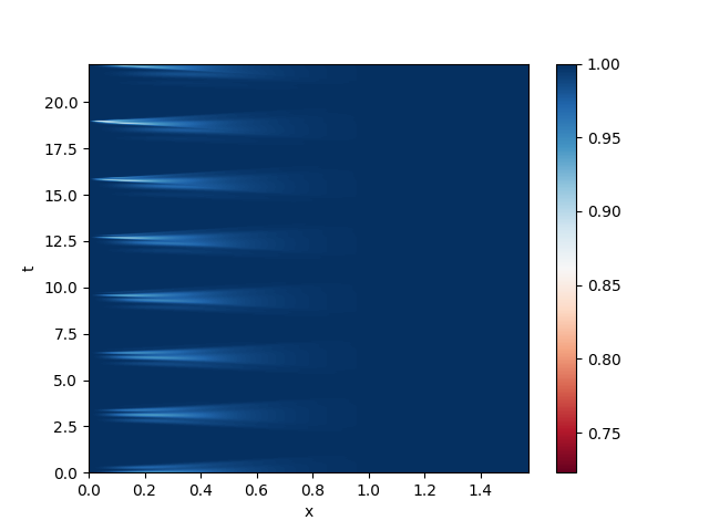
(a) $A(t,x)$

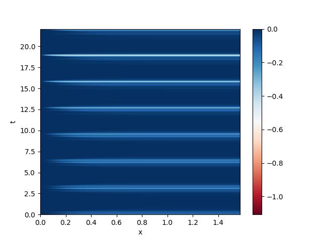
(b) $\delta(t,x)$

Figure 1: Metric functions for collapse of a massless scalar in AdS₅ with initial width $\sigma=0.25$ and amplitude $a=3.87$

The closest equivalent to the thin shell Vaidya spacetime is to inject a scalar field pulse at the conformal boundary via time-dependent boundary conditions for $\phi$. However, based on the experience of deppefreyhoult , numerical convergence fails even at relatively short times for $n<15$. Therefore, we instead require that $\phi(t,\pi/2)\to 0$ (with the appropriate fall off for normalizable modes) and take initial data such that the canonical momentum is Gaussian in the radius,

$$\Pi(t=0,x)=a\exp\left(-\frac{\tan^{2}(x)}{\sigma^{2}}\right),\quad\phi(t=0,x)=0.$$ (6)

We use linear interpolation to find values of $A(t,x),\delta(t,x)$ (as well as scalar field quantities) between spatial grid points and time steps for use in calculating the complexities as described below. Figure 1 shows the metric functions $A(t,x),\delta(t,x)$ for an example set of the initial data that forms a horizon after the scalar pulse reflects from the conformal boundary seven times. Each time the pulse approaches the origin (when $t$ is a multiple of $\pi$), the minimum value of $A$ gets smaller and $\delta$ becomes more negative (for all $x$); this effect intensifies each time. From this point of view, the pulse focuses as time goes on, which suggests that the complexity may ratchet to progressively larger (or even smaller) values during the pre-collapse phase of scalar field evolution.

3 Complexity as Volume

3.1 Set-Up

We recall that the volume complexity of the boundary CFT state on a spacelike slice $\Sigma$ is given by $\mathcal{C}_{V}=\max[V(\mathcal{B})/G\ell]$, where the maximum is taken over surfaces $\mathcal{B}$ such that $\partial\mathcal{B}=\Sigma$ and $\ell$ is a specified length scale. In most cases, $\ell$ is taken to be the AdS curvature radius ($=1$ in our units), but it is $\ell=r_{+}$ the Schwarzschild radius for small black holes in AdS. In this way, $\ell$ is the maximal time to fall from the horizon to the final cylinder in either a large or small black hole arXiv:1807.02186 . While it is unclear how to generalize the relationship described by this prescription to a dynamical setting, we consider initial conditions that eventually lead to small black holes and therefore (for most of our discussion) take $\ell=r_{+,f}$, the Schwarzschild radius of the final equilibrium black hole after all the initial energy falls behind the horizon. However, we discuss the alternate prescription taking $\ell=1$ below as well.

Because the asymptotically AdS_d+1 metric (2) is spherically symmetric, the maximal volume surface is a surface of revolution obtained by rotating the curve $(t(\lambda),x(\lambda))$ around the $S^{d-1}$ with the boundary condition $x(\lambda\to\infty)\to\pi/2$. The value of $t(\lambda\to\infty)$ is the time at which we measure the complexity. The volume of any such surface is

$$V=\frac{2\pi^{(d-1)/2}}{\Gamma((d-1)/2))}\int d\lambda\,\tan^{(d-1)}(x)\sec(x)\sqrt{(x^{\prime})^{2}A^{-1}-(t^{\prime})^{2}Ae^{-2\delta}},$$ (7)

where a prime indicates the derivative with respect to $\lambda$. We can choose the parameter $\lambda$ to set the integrand of (7) equal to unity, in which case the Euler-Lagrange equations have a first-order form

$$(P^{x})^{\prime} =-(P^{x})^{2}\left(\frac{A_{x}}{2\Omega}\right)-(P^{t})^{2}\left(\frac{e^{2\delta}}{2A^{2}\Omega}\right)(A_{x}-2A\delta_{x})+(d-1)\cot(x)+d\tan(x),$$ (8)

$$(P^{t})^{\prime} =-(P^{x})^{2}\left(\frac{A_{t}}{2\Omega}\right)-(P^{t})^{2}\left(\frac{e^{2\delta}}{2A^{2}\Omega}\right)(A_{t}-2A\delta_{t}),$$ (9)

$$x^{\prime} =\left(\frac{A}{\Omega}\right)P^{x},\quad\textnormal{and}\quad t^{\prime}=-\left(\frac{e^{2\delta}}{A\Omega}\right)P^{t},$$ (10)

where subscript $x,t$ denote partial derivatives and $\Omega\equiv\tan^{2(d-1)}x\sec^{2}x$. With the given choice of parameter,

$$\sqrt{\frac{A(P^{x})^{2}-A^{-1}e^{2\delta}(P^{t})^{2}}{\Omega}}=1.$$ (11)

For the surface to be smooth at the origin, $dt/dx=0$, which implies $e^{2\delta}P^{t}/A^{2}P^{x}\to 0$ as $x\to 0$. Then our choice of parameter implies $P^{x}\approx\sqrt{\Omega/A}$ and $x^{\prime}\approx\sqrt{A/\Omega}$, while the Einstein equation constraints imply that $A\approx 1+a(t)x^{2}$ near the origin. Therefore, to the first subleading order,

$$\lambda=\frac{1}{d}x^{d}+3\left(\frac{d-1/2}{d+2}\right)x^{d+2}+\frac{1}{2(d+2)}x^{d}\left(A(t,x)-1\right).$$ (12)

Meanwhile, equation (9) yields $dP^{t}/dx\approx-A_{t}/2$, so

$$P^{t}=-\frac{1}{2(d+2)}A_{t}(x,t)x^{d}$$ (13)

to order $x^{d+2}$. To this order, $t$ is constant. We can therefore solve (8,9,10) starting from a given $t_{0}$ and $x_{0}\ll 1$ using (12,13) as initial values at $x_{0}$.

Near the conformal boundary, $A_{x},A_{t}\to 0$, while $\delta\to\delta(t)$. As a result, we have a self-consistent solution with $(P^{x})^{\prime}\approx d\tan(x)$, or $P^{x}\approx\sqrt{\Omega}$ to leading order. In particular, this means that $x^{\prime}\approx 1/\sqrt{\Omega}$, so the surface requires an infinite parameter $\lambda$ to reach the boundary. We therefore cut off the surface at $x=\pi/2-\epsilon$. The value of $t$ at this point is not quite the value at the boundary; however, the difference is $\mathcal{O}(\epsilon^{d+1})$, so we neglect it.

3.2 Methods and Results

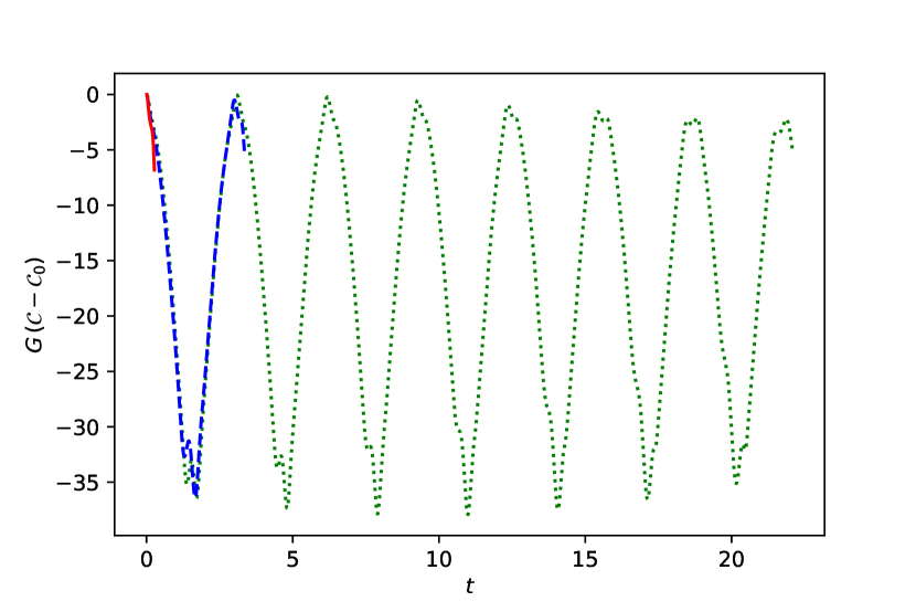
(a) AdS₅, $\mu=0$, $\sigma=0.25$, $a=8.28,6.39,3.87$

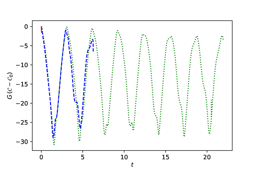
(b) AdS₄, $\mu=0$, $\sigma=0.25$, $a=15,8.0,5.0$

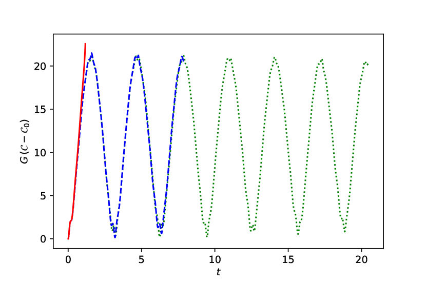
(c) AdS₅, $\mu=5$, $\sigma=2$, $a=0.38,0.12,0.10$

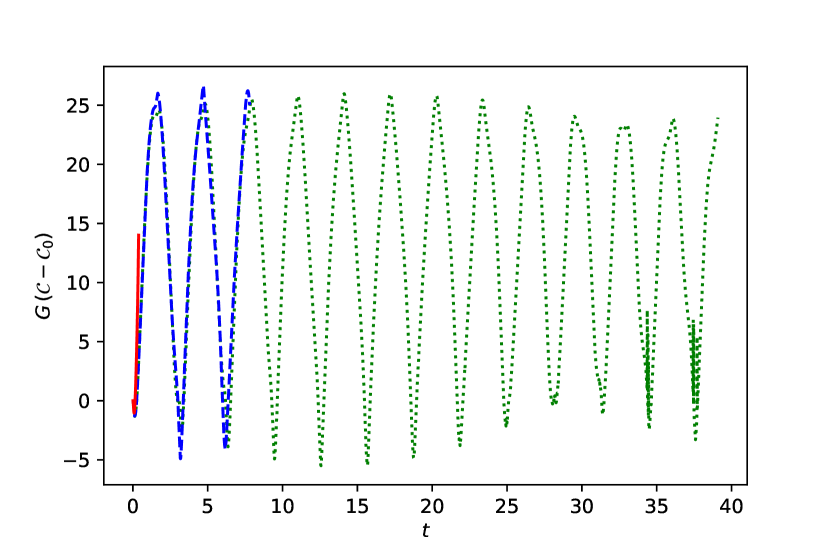
(d) AdS₄, $\mu=0$, $\sigma=8$, $a=1.00,0.14,0.10$

Figure 2: Volume complexity for listed initial data in AdS₄ and AdS₅. Curve for the largest amplitude in each figure is solid red, middle is dashed blue, smallest is dotted green.

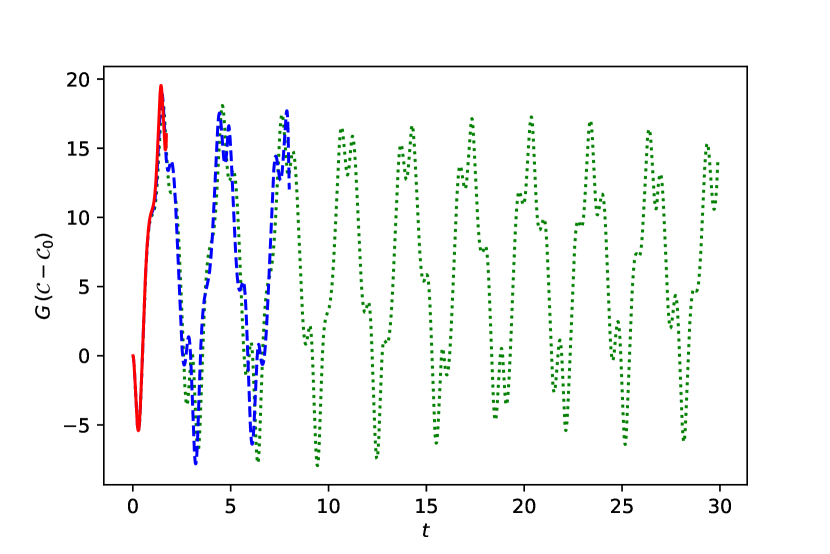
(a) $\mathcal{C}$ vs $t$: $\sigma=2.1$, $a=0.28,0.24,0.18$

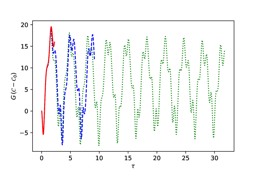
(b) $\mathcal{C}$ vs $\tau$: $\sigma=2.1$, $a=0.28,0.24,0.18$

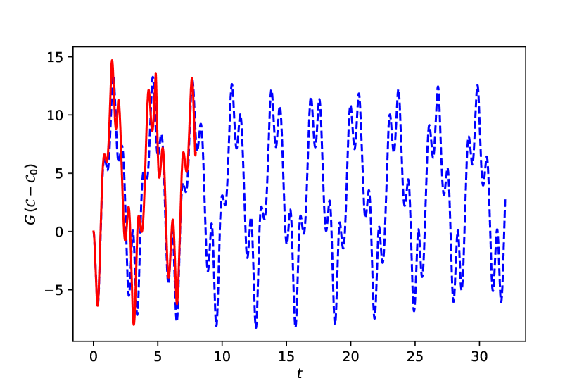
(c) $\mathcal{C}$ vs $t$: $\sigma=1.7$, $a=0.38,0.22$

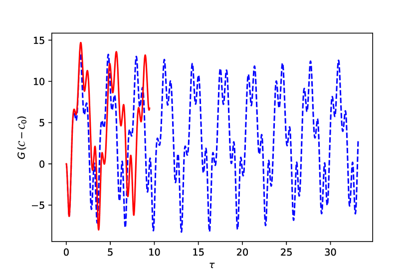
(d) $\mathcal{C}$ vs $\tau$: $\sigma=1.7$, $a=0.38,0.22$

Figure 3: Volume complexity vs $t$ and $\tau$ for two sets of initial data. Both are massless scalars in AdS₅. Curve for the largest amplitude in each figure is solid red, next is dashed blue, and next is dotted green.

To find the maximal volume, we integrate the Euler-Lagrange equations using the odeint function of the Python scipy library, reading in the outputs of the scalar field collapse simulations. We interpolate those functions as described in our discussion of figure 1 at the end of section 2.2; we find partial derivatives of $A,\delta$ through differencing.

We determine the volume by finding the value of $\lambda$ where $x=1.55$ at a time given by the value of $t$ on the surface at $x=1.55$, which can alternately be given in terms of the conformal boundary time $\tau$ at that same point. The complexity at this time is

$$G\mathcal{C}=\left(\frac{2\pi^{(d-1)/2}}{\Gamma(\frac{d-1}{2})}\right)\left(\frac{4\pi}{(d-1)\mathcal{M}}\right)\lambda(x=1.55)=\left(\frac{4\pi}{(d-1)\mathcal{M}}\right)V,$$ (14)

where the mass gives the final equilibrium black hole Schwarzschild radius with our normalization for the scalar field. To isolate the time dependence of the complexity, we subtract $\mathcal{C}_{0}$, the value at $t=\tau=0$. That is, while we regulated the divergent volume by cutting it off at radial coordinate $x=1.55$, we display the time dependence by renormalizing away the initial value of the volume, which is just the empty AdS value plus an $\mathcal{O}(a^{2})$ correction. We also note that the factor of $\mathcal{M}$ in the denominator appears because we take $\ell=r_{+}$ in the definition of complexity. Since the conserved mass $\mathcal{M}$ is proportional to $a^{2}$ at small amplitudes (due to backreaction, the relationship is not so clean at larger amplitudes), converting to the prescription where $\ell$ is the AdS radius roughly scales $\mathcal{C}$ by $a^{2}$.

Figure 2 shows examples of volume complexity curves as a function of origin time $t$ for a variety of initial data as listed in the captions. Each curve terminates when the evolution satisfies our approximate criterion for horizon formation. There are several features in common for all the complexity curves, including for a massive scalar field. First, the complexity appears quasiperiodic without a clear increasing or decreasing trend (other than possibly a weak modulation in the amplitude of complexity flucuations for the smallest scalar field amplitudes). Second, we note that the complexity is near its maximum value at $t=0$ for initial scalar profiles of width less than the AdS scale, while it is near its minimum at $t=0$ for widths larger than the AdS scale. Finally, and strikingly, the fluctuation of the complexity as a function of origin time $t$ is nearly independent of the scalar field amplitude $a$ until shortly before horizon formation. On the other hand, the time of the dual field theory is the conformal boundary time $\tau$, which does not scale in a simple way with $a$. Figure 3 shows the complexity for two sets of initial data plotted against origin time $t$ (subfigures 3(a),3(c)) and against conformal boundary time $\tau$ (subfigures 3(b),3(d)). As figure 1(b) suggests, the $\mathcal{C}(\tau)$ curves are stretched compared to the $\mathcal{C}(t)$ curves, with stretching more pronounced shortly before formation of a horizon. As a result, the curves for larger initial amplitudes are stretched more at earlier times than the $\mathcal{C}(\tau)$ for smaller $a$, and the complexity curves no longer align.

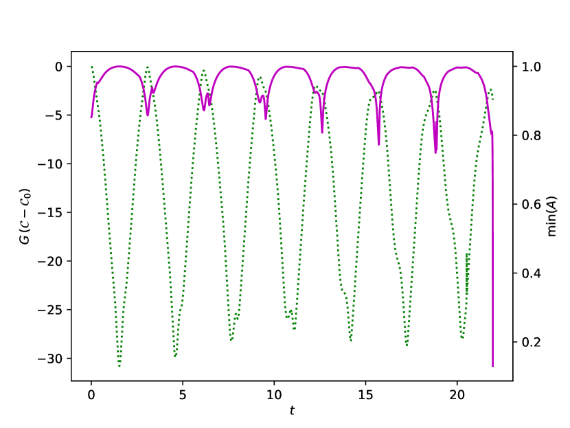
(a) $\sigma=0.25$, $a=5.0$

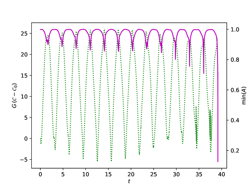
(b) $\sigma=8$, $a=0.10$

Figure 4: Volume complexity and minimum $A(x)$ vs $t$ for two sets of initial data. Both are massless scalars in AdS₄. Complexity is dotted green and minimum $A$ is solid magenta. The scales are shown on the left and right vertical axes respectively.

We can understand the oscillatory behavior of the complexity in terms of the complexity-momentum correspondence proposed in Susskind:2018tei and proved for volume complexity in spherically symmetric spacetimes in Barbon:2020olv . In the evolutions presented here, the energy of the scalar field is concentrated in thick shells (which may separate at times into thinner shells that nonetheless travel together). According to the complexity-momentum correspondence, the complexity should increase as the shells travel inward (the momentum is infalling) and decrease as the shells travel outward. Therefore, the complexity should be at a local maximum in time when the shells are closest to the origin. To see that this happens here, we redisplay the complexity of the smallest amplitude evolutions from figures 2(b) and 2(d) in figure 4 alongside the minimum with respect to $x$ of the metric function $A(t,x)$. We see that the local maxima of the complexity align with the local minima (in time) of $A$, which occur when the scalar pulse is most localized near the origin, as expected. The narrow initial data ($\sigma<1$) start at maximum complexity because the energy of the scalar field is initially concentrated near the origin, whereas wide initial data ($\sigma>1$) has energy initially in a shell located at large radius, which then falls toward the origin. Note that figure 4 does not distinguish the contribution of $A$ from that of $\delta$ to the complexity, since they are both most extreme at the same times, though the fact that the maximal volume surface is nearly a constant time surface hints that $A$ is more important.

It is also worth pondering the origin of the near amplitude independence of the fluctuations of the complexity. From the gravitational side of the duality, the rough scaling is relatively straightforward to understand at least for $a\ll 1$: both $\delta$ and $A-1$ are $\mathcal{O}(a^{2})$, so the time dependence of the volume $V$ must also be $\mathcal{O}(a^{2})$, so the change in complexity is invariant for the $\ell=r_{+}$ prescription. However, this relationship is more mysterious from the point of view of the dual field theory. Since the backgrounds are related by rescaling the scalar field and therefore the expectation value of the dual operator $\mathcal{O}_{\phi}$, conformal invariance seems to play a role. On first glance, that would seem also to explain why the time scale of smaller amplitudes is somewhat stretched in boundary time $\tau$, leading to alignment when plotted against origin time. This is problematic, though, since $\tau-t\sim\mathcal{O}(a^{2})$ at small amplitudes, but the near amplitude invariance holds for massive as well as massless scalars, which correspond to operators with different scaling dimensions. On the other hand, we could also consider the prescription with $\ell=1$, the AdS radius. Then the initial value $\mathcal{C}_{0}$ is (very close to) the ground state complexity in each case. If the scalar field background corresponds to an $\mathcal{O}(a)$ perturbation of the CFT state that is perpendicular to the vector from the reference state to the ground state (with regard to the appropriate metric for complexity), $\mathcal{C}-\mathcal{C}_{0}$ will scale like $a^{2}$. Then figure 2 has the demonstrated amplitude invariance. (This is a similar argument to that of arXiv:1806.08376 ; arXiv:1902.06499 ; arXiv:1903.04511 .)

If it holds as the amplitude vanishes, the scaling of complexity fluctuations allows us to comment on the validity of Lloyd’s bound, $|d\mathcal{C}/d\tau|\lesssim\mathcal{M}$, which Engelhardt:2021mju proved recently for volume complexity with $\ell=1$. In particular, the validity of Lloyd’s bound depends on the reference scale $\ell$ chosen in the definition of $\mathcal{C}_{V}$. First, in the $\ell=r_{+}$ prescription, $d\mathcal{C}/dt$ is unchanged as $a\to 0$, and it becomes the left-hand-side of Lloyd’s bound since $\tau\to t$ in that limit. On the other hand, $\mathcal{M}\to 0$, so Lloyd’s bound must be violated in the small amplitude limit. In contrast, for $\ell=1$, both $d\mathcal{C}/d\tau$ and $\mathcal{M}$ scale as $a^{2}$, so our results are parametrically consistent with Lloyd’s bound. This result may be a point in favor of using the AdS scale as the reference length in volume complexity.

The initial data shown in figures 2,3(a),3(b) exhibit instability toward black hole formation at all computationally accessible amplitudes (and also demonstrate the perturbative scaling $t_{H}\propto a^{-2}$ at small enough amplitudes) arXiv:1711.00454 . We confirm that the time dependence of the complexity has the same three behaviors for initial data that is stable against horizon formation at low amplitudes in figures 3(c),3(d). In these figures, the solid red curve represents an amplitude that forms a horizon at $t_{H}\approx 8$, while the dashed blue curve displays the complexity for a smaller amplitude that does not form a horizon until at least $t=500$ (however, we display only until $t=35$ to reduce data storage requirements). In other words, prior to horizon formation, the volume complexity is sensitive to eventual stability or instability only through the difference in origin and conformal boundary times.

As a final point, the reader may notice that $\mathcal{C}-\mathcal{C}_{0}$ can take negative values. On the other hand, Engelhardt:2021mju proved recently that volume complexity is always greater than the value for empty AdS, given a few assumptions. This apparent discrepancy is due to the contribution of the initial scalar field configuration to $\mathcal{C}_{0}$. We have verified by numerical comparison that the minimum complexity for each of our evolutions is in fact greater than the complexity of empty AdS, so our results are consistent with Engelhardt:2021mju .

4 Complexity as Action

4.1 Set-Up

The action complexity of the state on a fixed time slice $\Sigma$ of the boundary is $\mathcal{C}_{A}=S_{WDW}/\pi$, where $S_{WDW}$ is the action of the Wheeler–DeWitt patch of $\Sigma$ in the bulk AdS spacetime, including terms on the boundary of the WDW patch. Specifically, the WDW patch action is $S_{WDW}=S+S_{f}+S_{p}+S_{j}$, where $S$ is the bulk action given in equation (1), $S_{f,p}$ are boundary terms on the lightsheets bounding the past and future of the WDW patch, and $S_{j}$ is a joint term at the intersection of the two lightsheets. The lightsheet contributions are

$$S_{f,p}=\pm\frac{1}{8\pi G}\int d\lambda d^{d-1}\theta\sqrt{\gamma}\left(\kappa+\Theta\ln(\ell_{ct}\Theta)\vphantom{\frac{1}{2}}\right)$$ (15)

over the future- or past-directed lightsheet emitted from $\Sigma$, where $\lambda$ is a future-directed lightlike coordinate along the lightsheet, $\theta$ are angular coordinates on the lightsheet, $\gamma$ is the determinant of the induced metric on the fixed-$\lambda$ slices, $k^{\mu}$ is the normal (and therefore tangent or along $\lambda$) to the null hypersurface, $\kappa$ can be defined by $k^{\nu}\nabla_{\nu}k^{\mu}=\kappa k^{\mu}$, $\Theta\equiv\partial_{\lambda}\ln\sqrt{\gamma}$ is the expansion of the lightsheet, and $\ell_{ct}$ is an arbitrary lengthscale for the expansion counterterm. The lightsheet and joint terms make the variational problem well-defined within the WDW patch, as well as making the action parameterization invariant arXiv:1609.00207 ; arXiv:1804.07410 demonstrated the importance of the lightsheet expansion term to the action complexity. The joint term is

$$S_{j}=-\frac{1}{8\pi G}\int d^{d-1}\theta\sqrt{\sigma}\left(\vphantom{\frac{1}{2}}\ln(-k_{f}\cdot k_{p}/2)\right),$$ (16)

where $\sigma$ is the determinant of the induced metric on the joint and $k_{f,p}$ are the normals to the future- and past-directed lightsheets intersecting at the joint. Since the scalar fields we consider have $m^{2}\geq 0$, we do not include lightsheet or joint terms for the scalar following arXiv:1903.04511 ; arXiv:2002.05779 (see also arXiv:1901.00014 for a discussion of boundary terms for scalars).

Like the volume complexity, the action diverges due to contributions near the conformal boundary. To regulate it, we define the past and future boundaries of the WDW patch as lightsheets joining at $t=t_{0}$, $x=\pi/2-\epsilon$ for some small $\epsilon$. Then we use the lightlike coordinates $\lambda=x$ on the past boundary of the WDW patch and $\lambda=\pi/2-x$ on the future boundary, so $\lambda$ increases toward the future. Then the past and future boundaries of the WDW patch are described by $dt_{p,f}/dx=\pm\exp(\delta)/A$ respectively. The on-shell bulk action is therefore

$$S=\frac{1}{16\pi G}\left(\frac{2\pi^{(d-1)/2}}{\Gamma(\frac{d-1}{2})}\right)\int_{0}^{\pi/2-\epsilon}dx\int_{t_{p}(x)}^{t_{f}(x)}dt\,\tan^{d-1}(x)\sec^{2}(x)e^{-\delta(t,x)}\left(-2d+2\mu^{2}\phi^{2}\right)$$ (17)

with our choice of coordinates. The lightsheet contributions give

$$S_{f}+S_{p} =\frac{1}{8\pi G}\left(\frac{2\pi^{(d-1)/2}}{\Gamma(\frac{d-1}{2})}\right)\int_{0}^{\pi/2-\epsilon}dx\,\tan^{d-1}(x)\left[\partial_{x}\delta(t_{p}(x),x)+\partial_{x}\delta(t_{f}(x),x)\vphantom{\frac{e^{\delta}}{A}}\right.$$

$$\left.+\left(\frac{e^{\delta}\partial_{t}A}{A^{2}}\right)(t_{p}(x),x)-\left(\frac{e^{\delta}\partial_{t}A}{A^{2}}\right)(t_{f}(x),x)\right].$$ (18)

Note that the counterterms cancel for the two lightsheets because neither $A$ nor $\delta$ enters into the angular metric (a consequence of spherical symmetry). The joint term is

$$S_{j}=-\frac{1}{8\pi G}\left(\frac{2\pi^{(d-1)/2}}{\Gamma(\frac{d-1}{2})}\right)\cot^{d-1}(\epsilon)\ln\left[\csc^{2}(\epsilon)/A\right]\approx\frac{1}{8\pi G}\left(\frac{2\pi^{(d-1)/2}}{\Gamma(\frac{d-1}{2})}\right)\epsilon^{1-d}\left[2\ln\epsilon+\ln A\right].$$ (19)

The metric function $A$ has the expansion $A=1-2\mathcal{M}\epsilon^{d}/(d-1)+\mathcal{O}(\epsilon^{d+2})$ near $x=\pi/2$, so, while $S_{j}$ diverges for $\epsilon\to 0$, the time-dependence (and in fact the entire deviation from empty AdS) vanishes in that limit.

4.2 Methods and Results

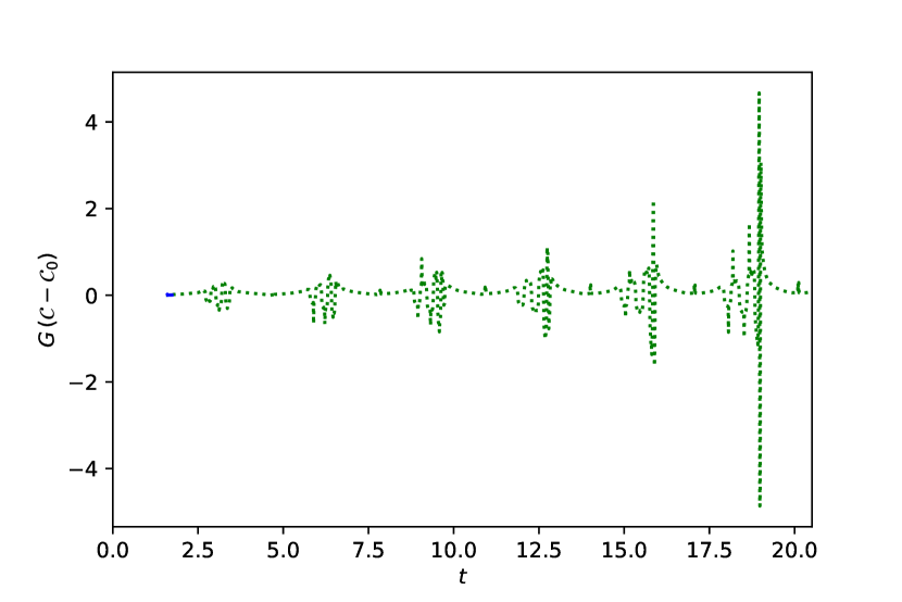
(a) AdS₅, $\mu=0$, $\sigma=0.25$, $a=6.39,3.87$

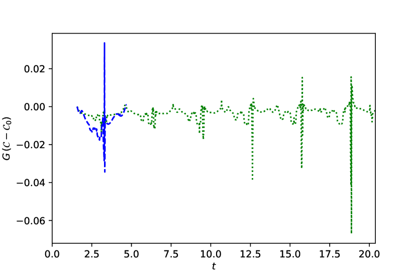
(b) AdS₄, $\mu=0$, $\sigma=0.25$, $a=15,8.0,5.0$

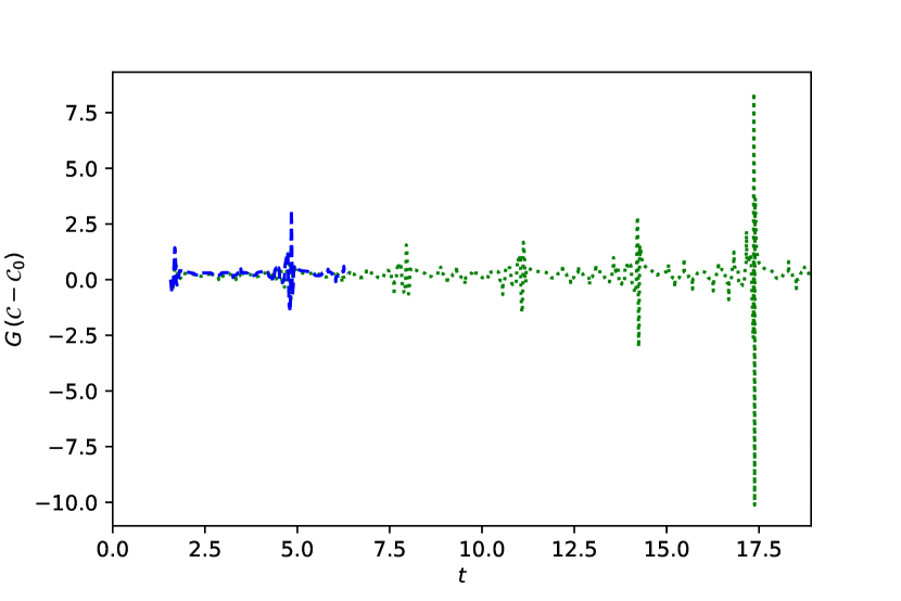
(c) AdS₅, $\mu=5$, $\sigma=2$, $a=0.12,0.10$

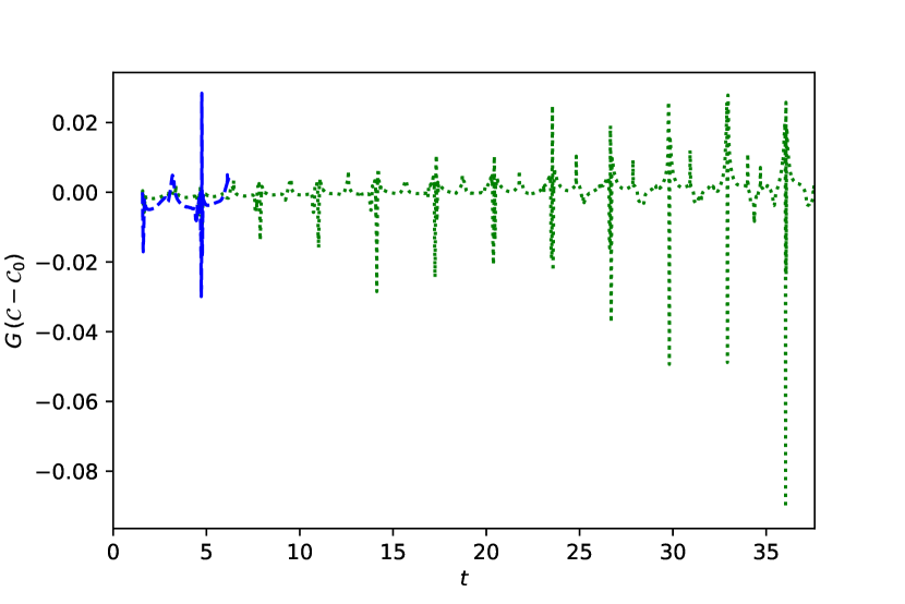
(d) AdS₄, $\mu=0$, $\sigma=8$, $a=0.14,0.10$

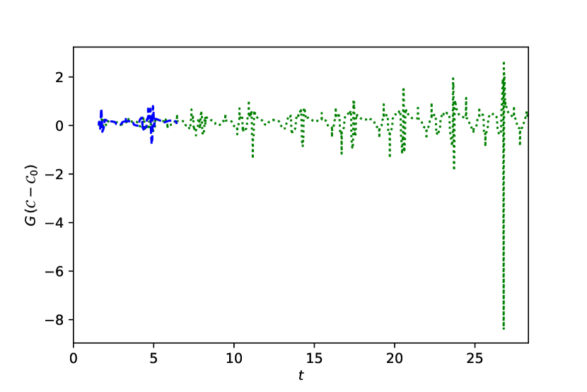
(e) AdS₅, $\mu=0$, $\sigma=2.1$, $a=0.24,0.18$

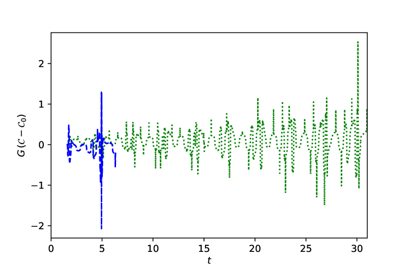
(f) AdS₅, $\mu=0$, $\sigma=1.7$, $a=0.38,0.22$

Figure 5: Rescaled action complexity for listed initial data in AdS₄ and AdS₅. Curve for the larger amplitude in each figure is dashed blue, smaller is dotted green.

To find the past and future boundaries $t_{p}(x),t_{f}(x)$ of the WDW patch, we again use the scipy function odeint, and we carry out the integrals (17,18) using the quad and nquad integration routines from scipy. To prevent errors in the bulk integral, we raised the number of nquad subdivisions to $5\times 10^{5}$ from the default value of 50. Just as for the volume complexity calculation, we interpolate the functions $A,\delta$ as necessary and evaluate derivatives through differencing. However, the complexity is evaluated at the time $t_{0}=t_{p}(\pi/2-\epsilon)=t_{f}(\pi/2-\epsilon)$ and $t_{p,f}(0)\approx t_{0}\pm\pi/2$, so we can only evaluate the complexity over the approximate range $\pi/2\lesssim t_{0}\lesssim t_{H}-\pi/2$. For other times, the WDW patch extends outside the region of spacetime we have simulated.

Figure 5 shows the action complexity for the same sets of initial data as figures 2 and 3. Because evaluating the complexity at time $t_{0}$ on the boundary cutoff surface requires bulk data for times $t_{0}-\pi/2\leq t\leq t_{0}+\pi/2$, the curves terminate at $t_{0}\approx t_{H}-\pi/2$. As a result, we do not evaluate the action complexity for the largest amplitude in each set of initial data when those form a horizon before $t=\pi/2$. Furthermore, since the behavior is similar (just stretched horizontally) when plotted versus boundary time $\tau$, we show only the $\mathcal{C}$ vs $t$ plots.

In each case, the complexity is roughly constant when averaged over a period of the scalar field oscillations, though there are pronounced spikes each period. Furthermore, while the complexity does not appear to have a trend on average, the spikes do increase in magnitude, especially near horizon formation. In fact, the spike size also increases somewhat for the smaller amplitude in figure 5(f), which is a stable evolution. We have verified that the dominant contribution to the time dependent complexity is the bulk integral and that the large spikes in $\mathcal{C}$ are at times when the scalar field pulse is passing through the origin; the spikes are due to greater time dilation effects since $\delta$ is most negative at those times. Therefore, we see that the progressive focusing of the scalar pulse as seen in the time dilation function $\delta$ also leads to a ratcheting effect in the magnitude of the spikes in the action complexity.

It is also worth noting that the action complexity for given width initial data has a similar shape for different initial scalar amplitudes; however, the action complexity does not have the same amplitude independence that we have seen for volume complexity. In fact, we have also checked whether this amplitude independence appears if we rescale the complexity by the square amplitude, but it does not.

5 Discussion

We have computed the holographic complexity of scalar field matter in the process of gravitational collapse prior to (an approximate notion of) black hole horizon formation using both $\mathcal{C}=V$ and $\mathcal{C}=A$ proposals. In contrast to black hole formation by thin shells in AdS-Vaidya spacetimes, the matter distributions we study are smooth and may not form a horizon until times late compared to the AdS scale. However, because our numerical solutions to the Klein-Gordon and Einstein equations are restricted to times before horizon formation, we are limited to studying early time transients in the complexity. In terms of the AdS/CFT correspondence, these backgrounds are dual to thermalization of an initial energy distribution (strictly speaking, we mean distribution of energy through modes of the CFT with a large range of scales). Therefore, our results indicate the time dependence of complexity during the approach to equilibrium of a CFT.

In global AdS coordinates, a time slice of the boundary is a sphere, so we might expect any energy in the CFT to equilibrate eventually because it cannot dissipate. In fact, if the initial scalar field profile is either wide or narrow compared to the AdS width, the scalar field matter appears to form a black hole even at arbitrarily small amplitudes. The intuition, supported by the time evolution of some metric components, is that the scalar field undergoes gravitational focusing as it oscillates in the AdS, eventually collapsing. However, due to the high degree of symmetry of AdS, some initial scalar profiles are stable against horizon formation at small amplitudes with quasiperiodic time evolution. This dichotomy naturally leads us to ask if holographic complexity can provide a diagnostic of stability or instability against collapse before the moment of horizon formation. The answer appears to be in the negative, as neither the volume nor action complexity is qualitatively different for stable versus unstable initial field profiles. Another question of interest is whether complexity behaves quasiperiodically or exhibits a ratcheting effect (some trend imposed on oscillatory behavior) due to focusing of the scalar field pulse.

The volume complexity appears quasiperiodic in time; the amplitude of oscillations in complexity is modulated (particularly for smaller scalar field amplitudes), but there is not a clear trend. Further, the complexity starts near its maximum or minimum for initial data that is narrower or wider than the AdS scale respectively. Most strikingly, if we use the Schwarschild radius for the length scale $\ell$ in the definition of volume complexity, the complexity (with initial value subtracted) is nearly invariant under change of amplitude; with $\ell$ equal the AdS radius, fluctuations in complexity scale as the second power of the scalar field amplitude. The origin of this property on the gravitational side of the duality is clear, but it is somewhat more obsure from the point of view of the boundary CFT. It may be related to conformal invariance of the dual field theory or to orthogonality between the ground state and the fluctuation due to the scalar field. This scaling property means that Lloyd’s bound is violated if the reference scale is the Schwarzschild radius.

The action complexity is also quasiperiodic in nature, except for large spikes in $\mathcal{C}-\mathcal{C}_{0}$ once per period (with period $\Delta t\sim\pi$) and some smaller spikes in between. These large spikes correspond to strong deviations of the time dilation function $\delta$, which expand the portion of the WDW patch near the boundary. While the overall complexity curve appears quasiperiodic, the large spikes increase in magnitude, particularly as the system approaches horizon formation. That is, the action complexity demonstrates a ratcheting behavior, becoming more extreme as the scalar pulse undergoes gravitational focusing.

We close with a few words about the relation of this work to the discussion of holographic complexity for coherent states in arXiv:1903.04511 ; arXiv:1912.10436 ; arXiv:2002.05779 . Coherent states of the CFT are given by scalar fields in AdS, like we study here. We have considered the nonperturbative evolution of those scalar fields, including backreaction from gravity in AdS. In contrast, arXiv:1903.04511 ; arXiv:2002.05779 studied perturbative scalar field amplitudes to second order, which captures the gravitational effects of the field but not the backreaction on the field itself. Therefore, they cannot study the gravitational collapse of the field leading to horizon formation. On the other hand, the numerical demands of recreating the spacetime geometry mean that we are unable to consider perturbatively small scalar field amplitudes for long time intervals. It would be interesting in the future to compare a numerical study of scalar field evolution to the perturbative results of arXiv:1903.04511 ; arXiv:2002.05779 .

- (1) L. Susskind, Computational Complexity and Black Hole Horizons, Fortsch. Phys. 64 (2016) 24 [1403.5695].
- (2) D. Stanford and L. Susskind, Complexity and Shock Wave Geometries, Phys. Rev. D 90 (2014) 126007 [1406.2678].
- (3) A. R. Brown, D. A. Roberts, L. Susskind, B. Swingle and Y. Zhao, Holographic Complexity Equals Bulk Action?, Phys. Rev. Lett. 116 (2016) 191301 [1509.07876].
- (4) A. R. Brown, D. A. Roberts, L. Susskind, B. Swingle and Y. Zhao, Complexity, action, and black holes, Phys. Rev. D 93 (2016) 086006 [1512.04993].
- (5) M. A. Nielsen, A geometric approach to quantum circuit lower bounds, quant-ph/0502070.
- (6) M. A. Nielsen, M. R. Dowling, M. Gu and A. C. Doherty, Quantum computation as geometry, Science 311 (2006) 1133–1135 [quant-ph/0603161].
- (7) M. R. Dowling and M. A. Nielsen, The geometry of quantum computation, quant-ph/0701004.
- (8) R. Jefferson and R. C. Myers, Circuit complexity in quantum field theory, JHEP 10 (2017) 107 [1707.08570].
- (9) R. Khan, C. Krishnan and S. Sharma, Circuit Complexity in Fermionic Field Theory, Phys. Rev. D 98 (2018) 126001 [1801.07620].
- (10) L. Hackl and R. C. Myers, Circuit complexity for free fermions, JHEP 07 (2018) 139 [1803.10638].
- (11) L. Susskind and Y. Zhao, Switchbacks and the Bridge to Nowhere, 1408.2823.
- (12) M. Moosa, Evolution of Complexity Following a Global Quench, JHEP 03 (2018) 031 [1711.02668].
- (13) M. Alishahiha, A. Faraji Astaneh, M. R. Mohammadi Mozaffar and A. Mollabashi, Complexity Growth with Lifshitz Scaling and Hyperscaling Violation, JHEP 07 (2018) 042 [1802.06740].
- (14) D. S. Ageev, I. Y. Aref’eva, A. A. Bagrov and M. I. Katsnelson, Holographic local quench and effective complexity, JHEP 08 (2018) 071 [1803.11162].
- (15) S. Chapman, H. Marrochio and R. C. Myers, Holographic complexity in Vaidya spacetimes. Part I, JHEP 06 (2018) 046 [1804.07410].
- (16) M. Lezgi and M. Ali-Akbari, Complexity and uncomplexity during energy injection, Phys. Rev. D 103 (2021) 126024 [2103.05023].
- (17) P. Bizon and A. Rostworowski, On weakly turbulent instability of anti-de Sitter space, Phys. Rev. Lett. 107 (2011) 031102 [1104.3702].
- (18) D. Garfinkle and L. A. Pando Zayas, Rapid Thermalization in Field Theory from Gravitational Collapse, Phys. Rev. D 84 (2011) 066006 [1106.2339].
- (19) J. Jalmuzna, A. Rostworowski and P. Bizon, A Comment on AdS collapse of a scalar field in higher dimensions, Phys. Rev. D 84 (2011) 085021 [1108.4539].
- (20) D. Garfinkle, L. A. Pando Zayas and D. Reichmann, On Field Theory Thermalization from Gravitational Collapse, JHEP 02 (2012) 119 [1110.5823].
- (21) A. Buchel, S. L. Liebling and L. Lehner, Boson stars in AdS spacetime, Phys. Rev. D 87 (2013) 123006 [1304.4166].
- (22) M. Maliborski and A. Rostworowski, A comment on ”Boson stars in AdS”, 1307.2875.
- (23) M. Maliborski and A. Rostworowski, Lecture Notes on Turbulent Instability of Anti-de Sitter Spacetime, Int. J. Mod. Phys. A 28 (2013) 1340020 [1308.1235].
- (24) O. Evnin, Resonant Hamiltonian systems and weakly nonlinear dynamics in AdS spacetimes, Class. Quant. Grav. 38 (2021) 203001 [2104.09797].
- (25) H. Okawa, J. C. Lopes and V. Cardoso, Collapse of massive fields in anti-de Sitter spacetime, 1504.05203.
- (26) N. Deppe and A. R. Frey, Classes of Stable Initial Data for Massless and Massive Scalars in Anti-de Sitter Spacetime, JHEP 12 (2015) 004 [1508.02709].
- (27) B. Cownden, N. Deppe and A. R. Frey, Phase diagram of stability for massive scalars in anti–de Sitter spacetime, Phys. Rev. D 102 (2020) 026015 [1711.00454].
- (28) N. Deppe, A. Kolly, A. R. Frey and G. Kunstatter, Black Hole Formation in AdS Einstein-Gauss-Bonnet Gravity, JHEP 10 (2016) 087 [1608.05402].
- (29) V. Balasubramanian, A. Buchel, S. R. Green, L. Lehner and S. L. Liebling, Holographic Thermalization, Stability of Anti–de Sitter Space, and the Fermi-Pasta-Ulam Paradox, Phys. Rev. Lett. 113 (2014) 071601 [1403.6471].
- (30) P. Bizoń and A. Rostworowski, Comment on “Holographic Thermalization, Stability of Anti–de Sitter Space, and the Fermi-Pasta-Ulam Paradox”, Phys. Rev. Lett. 115 (2015) 049101 [1410.2631].
- (31) V. Balasubramanian, A. Buchel, S. R. Green, L. Lehner and S. L. Liebling, Reply to Comment on “Holographic Thermalization, Stability of Anti–de Sitter Space, and the Fermi-Pasta-Ulam Paradox”, Phys. Rev. Lett. 115 (2015) 049102 [1506.07907].
- (32) B. Craps, O. Evnin and J. Vanhoof, Renormalization, averaging, conservation laws and AdS (in)stability, JHEP 01 (2015) 108 [1412.3249].
- (33) A. Buchel, S. R. Green, L. Lehner and S. L. Liebling, Conserved quantities and dual turbulent cascades in anti–de Sitter spacetime, Phys. Rev. D 91 (2015) 064026 [1412.4761].
- (34) B. Craps, O. Evnin and J. Vanhoof, Renormalization group, secular term resummation and AdS (in)stability, JHEP 10 (2014) 048 [1407.6273].
- (35) P. Carracedo, J. Mas, D. Musso and A. Serantes, Adiabatic pumping solutions in global AdS, JHEP 05 (2017) 141 [1612.07701].
- (36) A. Biasi, P. Carracedo, J. Mas, D. Musso and A. Serantes, Floquet Scalar Dynamics in Global AdS, JHEP 04 (2018) 137 [1712.07637].
- (37) B. Cownden, Examining Instabilities Due to Driven Scalars in AdS, JHEP 12 (2020) 013 [1912.07143].
- (38) N. Deppe, A. Kolly, A. Frey and G. Kunstatter, Stability of AdS in Einstein Gauss Bonnet Gravity, Phys. Rev. Lett. 114 (2015) 071102 [1410.1869].
- (39) N. Deppe, A. R. Frey and R. E. Hoult, work in progress, .
- (40) J. Couch, S. Eccles, T. Jacobson and P. Nguyen, Holographic Complexity and Volume, JHEP 11 (2018) 044 [1807.02186].
- (41) L. Susskind, Why do Things Fall?, 1802.01198.
- (42) J. L. F. Barbon, J. Martin-Garcia and M. Sasieta, Proof of a Momentum/Complexity Correspondence, Phys. Rev. D 102 (2020) 101901 [2006.06607].
- (43) M. Flory and N. Miekley, Complexity change under conformal transformations in AdS3/CFT2, JHEP 05 (2019) 003 [1806.08376].
- (44) M. Flory, WdW-patches in AdS3 and complexity change under conformal transformations II, JHEP 05 (2019) 086 [1902.06499].
- (45) A. Bernamonti, F. Galli, J. Hernandez, R. C. Myers, S.-M. Ruan and J. Simón, First Law of Holographic Complexity, Phys. Rev. Lett. 123 (2019) 081601 [1903.04511].
- (46) N. Engelhardt and Å. Folkestad, General Bounds on Holographic Complexity, 2109.06883.
- (47) N. Engelhardt and Å. Folkestad, Negative Complexity of Formation: the Compact Dimensions Strike Back, 2111.14897.
- (48) L. Lehner, R. C. Myers, E. Poisson and R. D. Sorkin, Gravitational action with null boundaries, Phys. Rev. D 94 (2016) 084046 [1609.00207].
- (49) A. Bernamonti, F. Galli, J. Hernandez, R. C. Myers, S.-M. Ruan and J. Simón, Aspects of The First Law of Complexity, 2002.05779.
- (50) K. Goto, H. Marrochio, R. C. Myers, L. Queimada and B. Yoshida, Holographic Complexity Equals Which Action?, JHEP 02 (2019) 160 [1901.00014].
- (51) S. S. Hashemi, G. Jafari and A. Naseh, First law of holographic complexity, Phys. Rev. D 102 (2020) 106008 [1912.10436].