OSSOS. XXIII. 2013 VZ₇₀ and the Temporary Coorbitals of the Giant Planets

Abstract

We present the discovery of 2013 VZ₇₀, the first known horseshoe coorbital companion of Saturn. Observed by the Outer Solar System Origins Survey (OSSOS) for 4.5 years, the orbit of 2013 VZ₇₀ is determined to high precision, revealing that it currently is in ‘horseshoe’ libration with the planet. This coorbital motion will last at least thousands of years but ends $\sim 10$ kyr from now; 2013 VZ₇₀ is thus another example of the already-known ‘transient coorbital’ populations of the giant planets, with this being the first known prograde example for Saturn (temporary retrograde coorbitals are known for Jupiter and Saturn). We present a theoretical steady state model of the scattering population of trans-Neptunian origin in the giant planet region (2–34 au), including the temporary coorbital populations of the four giant planets. We expose this model to observational biases using survey simulations in order to compare the model to the real detections made by a set of well-characterized outer Solar System surveys. While the observed number of coorbitals relative to the scattering population is higher than predicted, we show that the number of observed transient coorbitals of each giant planet relative to each other is consistent with a transneptunian source.

1 Introduction

Coorbital objects are found in the 1:1 mean-motion resonance with a planet. Resonance membership is determined by inspecting the evolution of the resonant angle $\phi_{11}=\lambda-\lambda_{P}$, where $\lambda=\Omega+\omega+M$ is the mean longitude, $P$ denotes the planet, $\Omega$ is the longitude of the ascending node, $\omega$ the argument of pericenter and $M$ the mean anomaly. The resonant angle $\phi_{11}$ must librate rather than circulate (ie. $\phi_{11}$ must occupy a bounded range) in order for an object to be considered to be in coorbital resonance. Like other $n:1$ resonances, the 1:1 mean-motion resonance includes multiple libration islands; objects in these islands are called leading Trojans (mean $\langle\phi_{11}\rangle=+60\arcdeg$), trailing Trojans ($\langle\phi_{11}\rangle=300\arcdeg=-60\arcdeg$), quasi-satellites ($\langle\phi_{11}\rangle=0\arcdeg$) or horseshoe coorbitals ($\langle\phi_{11}\rangle=180\arcdeg$). The motion of Trojans librate around one of the L4 or L5 Lagrangian points, while the path of horseshoe coorbitals encompass all of the L3, L4 and L5 Lagrangian points; quasi-satellites appear to orbit the planet (while not actually being bound to it). Quasi-satellites and horseshoe coorbitals are almost always unstable and thus temporary (eg. Mikkola et al., 2006; Ćuk et al., 2012; Jedicke et al., 2018) with the exception of Saturn’s moons Epimetheus and Janus, which are horseshoe coorbitals of each other (Fountain & Larson, 1978). Greenstreet et al. (2020) and Li et al. (2018) discuss the existence of high inclination ($i>90\arcdeg$) objects temporarily trapped in a 1:-1 retrograde “coorbital” resonance with Saturn, although these are not coorbitals in the traditional sense described above; since they orbit the Sun in the opposite direction than the planet, retrograde coorbitals are not protected from close approaches with the planet the way that prograde coorbitals are, nor do the resonant island librations (ie. Trojan, horseshoe, quasi-satellite motion) behave in the traditional sense in the retrograde configuration.

For many planets, the coorbital phase space is unstable due to perturbations from neighboring planets (eg. Nesvorný & Dones, 2002; Dvorak et al., 2010). Innanen & Mikkola (1989) first suggested, at a time when only the Jovian Trojans were known, that populations of objects in stable 1:1 resonance with each of the other giant planets may exist; their analysis showed that the exact Lagrangian points are unstable for Saturn, but that Trojans farther from the resonance center (featuring larger libration amplitudes) could be stable for at least 10 Myr. These results were confirmed by Holman & Wisdom (1993). Using longer timescales than previous studies, de la Barre et al. (1996) specifically studied the stability of Saturnian Trojans and found that Saturnian Trojans could only be long-term ($>428$ Myr) stable with very specific conditions: very small eccentricity (<0.028), $\phi_{11}$ libration amplitude greater than $80\arcdeg$, $\omega$ libration about a point $45\arcdeg$ ahead of Saturn’s $\omega$, and constraints on the timing of the maximum eccentricity relative to the timing of Jupiter’s maximum eccentricity, so that Jupiter and the Trojans do not approach close enough to dislodge the Trojan from Saturn’s 1:1 resonance. Nesvorný & Dones (2002) showed that while Neptunian Trojans may have only been depleted by a factor of 2 over the age of the Solar System, the Saturnian Trojans would have been depleted by a factor of 100. Studying the cause of the instability of Saturnian Trojans, Marzari & Scholl (2000) and Hou et al. (2014) found that the instability is caused by interactions between mean motion and secular resonances. Given these destabilizing factors, causing any primordial population to have been mostly depleted and allowing only small niches to be long term stable, it is not surprising that no long-term stable Saturnian Trojans have been discovered to date.

Only Mars, Jupiter and Neptune have known populations of long-term ($>$Gyr) stable Trojans (which thus might be primordial) (Wolf, 1906; Bowell et al., 1990; Levison et al., 1997; Marzari et al., 2003; Scholl et al., 2005).

While only three planets are known to have long-term stable Trojans, scattering objects (scattering TNOs, Centaurs and even some objects originating in the asteroid belt) can become temporary coorbitals, transiently captured into unstable resonance (Alexandersen et al., 2013; Greenstreet et al., 2020). All Solar System planets except Mercury, Mars and Jupiter now have known populations of temporary coorbitals on prograde ($i<90\arcdeg$) orbits (Wiegert et al., 1998; Mikkola et al., 2004; Karlsson, 2004; Horner & Lykawka, 2012; Alexandersen et al., 2013; Greenstreet et al., 2020). Temporary “sticking” like this also occurs in other resonances (eg. Duncan & Levison, 1997; Tsiganis et al., 2000; Alvarez-Candal & Roig, 2005; Lykawka & Mukai, 2007; Yu et al., 2018; Volk et al., 2018).

Horner & Wyn Evans (2006) integrated the Centaurs known at the time, demonstrating that Centaurs do indeed get captured into temporary coorbital resonance with the giant planets, claiming that Jupiter should have by far the most temporary coorbitals, followed by Saturn and hardly any for Uranus and Neptune. Alexandersen et al. (2013) pointed out that using the known centaurs as the starting sample is biased towards having more objects nearer the Sun, and thus more captures for the inner giant planets, resulting in a disagreement with the sample of at-the-time known temporary coorbitals; they instead used a model that started with scattering TNOs that scatter inwards to become Centaurs and temporary coorbitals, to demonstrate that a TNO origin can explain the distribution of the temporary coorbitals of Neptune and Uranus.

In this paper we describe the discovery of the first known Saturnian horseshoe coorbital, 2013 VZ₇₀, and demonstrate its temporary nature (Section 2). Furthermore we expand upon the analysis of Alexandersen et al. (2013) to analyze the populations of temporary coorbitals of all four giant planets, in an attempt to demonstrate the likely origin of 2013 VZ₇₀ and similar objects. We use numerical integrations to construct a steady-state distribution model of the scattering Trans-Neptunian Objects (TNOs) and temporary coorbitals of the giant planets (Section 3). Lastly we use survey simulations, exposing our model to the survey biases of a well-understood set of surveys, in order to compare our theoretical predictions to real detections of this population (Section 4).

2 Observations and orbit of 2013 VZ₇₀

2013 VZ₇₀ was discovered by the Outer Solar System Origins Survey (OSSOS, Bannister et al., 2016, 2018) in images taken on 2013 November 1 using the MegaCam wide-field imager (Boulade et al., 2003) on the Canada-France-Hawai’i Telescope (CFHT). The object was subsequently measured in 37 tracking observations from 2013 August 09 to 2018 January 18 (for the full list of astrometric measurements, see MPEC 2021-Q55, Bannister et al., 2021). With 4.5 years of high-accuracy astrometry, the orbit is very well known, being $a=9.1838\pm 0.0002$ AU, $e=0.097145\pm 0.000011$, $i=12\arcdeg.04110\pm 0\arcdeg.00006$, $\Omega=215\arcdeg.22021\pm 0\arcdeg.00008$, $\omega=245\arcdeg.754\pm 0\arcdeg.006$, $M=291\arcdeg.425\pm 0\arcdeg.006$ for epoch = JDT 2456514.0. Here $a$, $e$, $i$ are the barycentric semi-major axis, eccentricity and inclination, respectively; the uncertainties are calculated from a covariance matrix using the orbit-fitting software Find_Orb (Gray, 2011). This orbit is very close to that of Saturn, although the two bodies are seperated by $\sim 180\arcdeg$ on the sky. From dynamical integrations we found that 2013 VZ₇₀ is in fact in the 1:1 mean motion resonance with Saturn, in a horseshoe configuration (see Figure 1). However, the best fit clone only remains resonant for about 11 kyr before leaving the resonance and re-joining the scattering population.

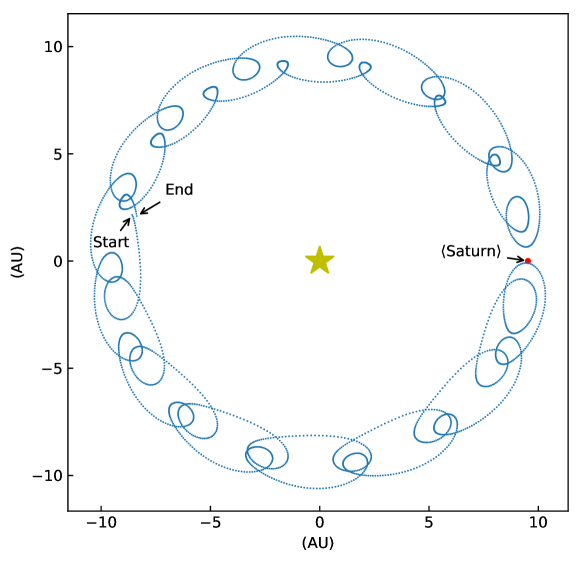
Figure 1: The forward integrated motion of 2013 VZ₇₀ for 1 libration period ($\sim 890$ yr at this instance), in the Saturnian mean-motion subtracted reference frame. The blue dots shows the motion of 2013 VZ₇₀ relative to Saturn’s mean motion (red dot). The start and end points are marked. The time between integration outputs (blue dots) is $\sim 0.33$ years. Note that when the object appears near Saturn in this planar, mean-motion subtracted projection, it is not actually close to the planet due to the vertical motion caused by the orbital inclination and the fact that Saturn’s true location does oscillate around the marked mean location.

We investigated whether the best fit orbit could be near a stability boundary by generating orbit clones from appropriate resampling of our astrometry, allowing us to test whether any orbit consistent with the astrometry featured long-term stability. Each clone was produced by resampling all the astrometry (using a normal distribution with standard deviation equal to the mean residual of the best fit, $0.\arcsec 146$) and fitting a new orbit. This process was repeated 10,000 times using Find_Orb. The distribution of orbits generated by this process explicitly shows how the uncertainty of some of the orbital parameters are strongly coupled, as can be seen in Figure 2. From these 10,000 clones, we identified the most extreme orbits (largest and smallest value of each parameter) and integrated these 8 clones (labelled in Figure 2) as well as the best fit orbit. These dynamical integrations were done using Rebound(Rein & Liu, 2012) with the WHFast(Wisdom & Holman, 1991; Kinoshita et al., 1991; Rein & Tamayo, 2015) symplectic integrator. The eight major planets and Pluto were included as massive perturbers and an integration step size of 5% of Mercury’s initial orbital period ($\simeq 0.012$ yr $\simeq 4.39$ days) was used, while output was saved approximately 3 times per year. As can be seen in Figures 3 and 4, the future evolution of all of the clones involve an initial period in coorbital resonance, but all clones leave the resonance between 6 kyr and 26 kyr from now. The large range of resonance exit times is due to the highly chaotic nature of the orbit. We used a second set of numerical integrations, where clones were displaced infinitesimally ($10^{-13}$–$10^{-12}$ AU, or 1.5–15 cm) relative to each of the above clones, to estimate the object’s current timescale for chaotic divergence (the Lyapunov time scale); we found this to be $410\pm 60$ yr. 2013 VZ₇₀ is thus definitely in coorbital resonance now, but the chaotic nature of the orbit means that the duration of this temporary resonance capture will likely not be constrained further, even with additional observations.

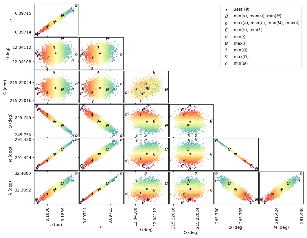
Figure 2: Orbital elements of 10,000 fits to resampled astrometry. Each clone was generated using Find_Orb’s MCMC feature, using a Gaussian noise equal to the mean residual of the best fit orbit ($0.\arcsec 146$). The clones are color coded by semi-major axis (which is also the x-axis of the left most row) to give an additional rough indicator of its correlation with the other orbital elements. The best fit orbit is marked with a black dot, and orbits with either the smallest or largest value of one of the parameters are marked with a letter ((a-h, not to be confused with any orbital elements). This figure demonstrates how the uncertainties on the different parameters are related; most parameters are strongly coupled, while $i$ and $\Omega$ have only weak or no coupling with other parameters.

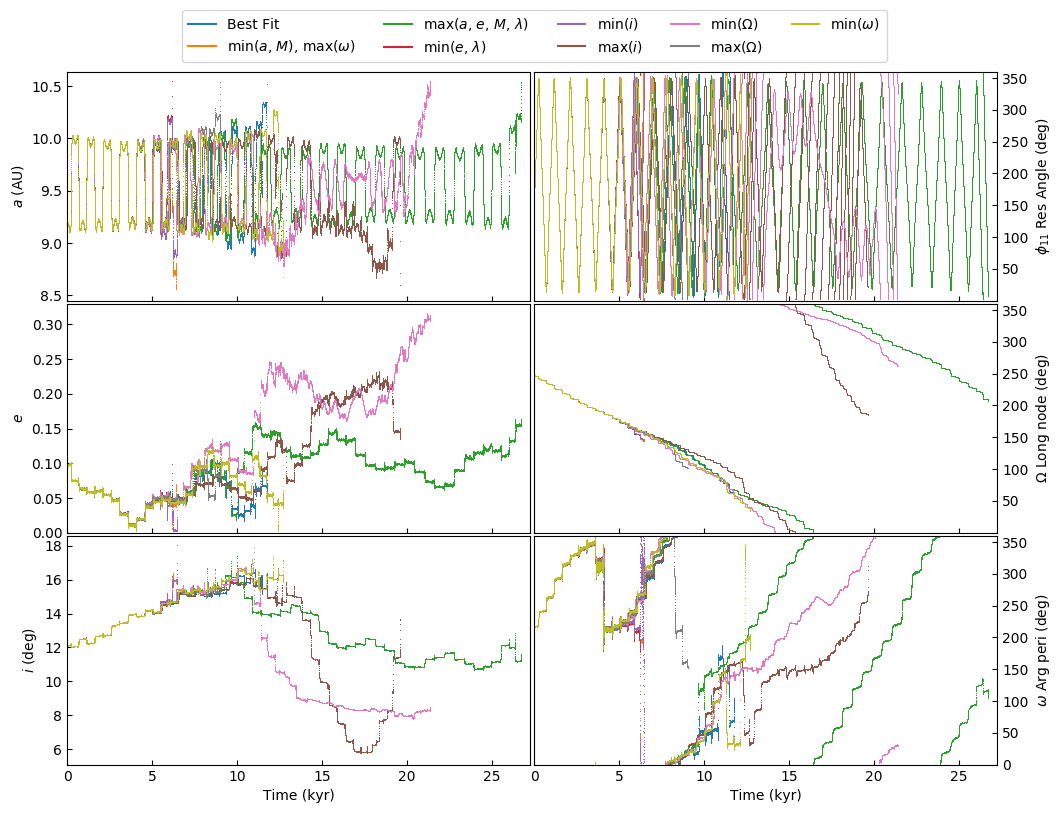
Figure 3: Future evolution of 2013 VZ₇₀, the temporary Saturnian horseshoe coorbital. The nine clones marked on Figure 2 were integrated (the best fit orbit plus eight extremal clones). For clarity, clone trajectories have only been drawn until the semi-major axis of the clone deviates from Saturn’s by more than 1 au for the first time. The top right panel has been expanded in Figure 4 to better show the clones’ interactions with the resonance. The "stair step" patterns occurs at the time when $\phi_{11}$ is close to $0\arcdeg/360\arcdeg$, which is the time the coorbital is closest to the planet; the close approach causes the switch from a slightly-larger-than-the-planet’s semi-major axis to a slightly-smaller-than-the-planet’s (and vice versa) that ensures that the planet/coorbital never overtake each other. The close approaches also imparts small changes in the other orbital elements, seen as the "stair step" pattern.

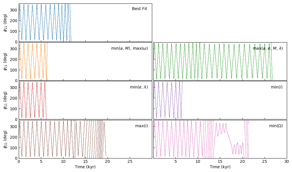
Figure 4: Future evolution of the resonant angle $\phi_{11}$ (with respect to Saturn) for each of the 2013 VZ₇₀ clones shown in Figures 2 and 3. The information here is identical to that in the top-right subplot of Figure 3, but split up for clarity. As in Figure 3, clone trajectories have only been drawn until the semi-major axis of the clone deviates from Saturn’s by more than 1 au for the first time. It is clear that 2013 VZ₇₀ is currently in the Saturnian coorbital resonance, but will escape from this state in 6–26 kyr. Note that after leaving the resonance, the minimum $\Omega$ clone gets recaptured and librates a few times in each Trojan island before becoming re-ejected.

3 Deriving the steady state orbital distribution

We proceed to investigate the potential origin of temporary coorbitals like 2013 VZ₇₀. We model the source of the giant planet temporary coorbitals and investigate their detectability in characterised surveys. We produced a steady-state distribution of scattering objects in the $a<34$ au region from orbital integrations similar to those used in Alexandersen et al. (2013); the details of those integrations can be found in the supplementary material of that paper. We primarily outline the deviations from those used in the previous paper below.

To perform the dynamical integrations, we used the N-body code SWIFT-RMVS4 (provided by Hal Levison, based on the original SWIFT (Levison & Duncan, 1994)) with a base time step of 25 days and an output interval of 50 years for the orbital elements of the planets and any particle which at the moment had $a<34$ au. The gravitational influences of the four giant planets and the Sun were included. The system starts with 8500 particles, derived from the 34 au $<a<$ 200 au scattering portion of the Kaib et al. (2011) model of the outer Solar System. Particles were removed from the simulation when they hit a planet, went outside 2000 AU or inside 2 AU from the Sun (since they would either interact with the terrestrial planets that are absent in our simulations or would rapidly be removed from the Solar System by Jupiter), or the final integration time of 1 Gyr was reached. As in Alexandersen et al. (2013) we confirm that the distribution in the first 100 Myr is similar enough to the distribution in the following 900 Myr (because the $a<$34 au region is populated very quickly despite starting off empty) that we can treat the distribution as a whole as being in steady state.

The method for determining coorbital behavior in the particle histories is also very similar to that used in Alexandersen et al. (2013), with some small modifications. To diagnose whether particles are coorbital, the orbital histories (at 50 year output intervals) were scanned using a running window 30 kyr long for Uranus/Neptune and 5 kyr long for Jupiter/Saturn; this window size was chosen to be several times longer than the typical Trojan libration period at the given planet ($\sim 1$ kyr for Saturn as seen in Figure 4). A particle was classified as a coorbital if, within the running window, both its average semimajor axis was less than 0.2 AU from the average semimajor axis of a given planet and no individual semimajor axis value deviated more than $R_{H}$ from that of the planet. Here $R_{H}$ is the planet’s Hill sphere radius (Murray & Dermott, 1999), where $R_{H}=0.35$  AU for Jupiter, $R_{H}=0.44$ AU for Saturn, $R_{H}=0.47$ AU for Uranus, and $R_{H}=0.77$ AU for Neptune. Further determination of which resonant island a coorbital is librating in was made identically to the method used in Alexandersen et al. (2013).

Our results are in good agreement with those for Uranus and Neptune in Alexandersen et al. (2013). Table 1 contains the fraction of the steady-state population in coorbital motion with each of the giant planets at any given time, as well as the distribution of coorbitals between horseshoe, Trojan and quasi-satellite orbits. The coorbital fraction for Uranus and Neptune are slightly higher than in Alexandersen et al. (2013), despite very similar methodology; however, these results agree within their expected accuracy. The capture fraction decreases from Neptune through to Jupiter (with almost 4000 times fewer coorbitals than Neptune), although this is unsurpring given that the source of the scattering objects is beyond Neptune and that the dynamical timescales (orbital period, libration timescale) are longer farther from the Sun. An interesting result is that while Neptune’s and Uranus’ coorbitals are roughly equally distributed between horseshoe and Trojan coorbitals, Saturn seems to very preferentially capture scattering objects into horseshoe orbits, and Jupiter has a much larger fraction of quasi-satellites than any of the other planets. Table 1 also shows the mean, median and maximum duration of a capture in coorbital resonance with the planets, as well as the mean, median and maximum number of captures experienced by particles with at least one episode of coorbital motion with a given planet. The mean and median coorbital lifetimes and number of captures for Uranus and Neptune are also within a factor of two of those in Alexandersen et al. (2013), which we thus adopt as the uncertainty. Note that the captures into coorbital motion with Saturn and Jupiter are typically significantly shorter than for Uranus and Neptune, although if the lifetimes are represented units of orbital periods rather than years, the Jovian captures actually have the second longest lifetimes, after Uranus. However, going Neptune to Jupiter, particles are increasingly unlikely to have multiple captures, presumably due to the increasing ability of the planet to scatter the object to large semi-major axis; this results in particles on average spending both more total time and more total orbital periods in coorbital motion with Uranus and Neptune than Saturn and Jupiter.

Table 1: Steady state fractions of the $a<34$ AU, $q>2$ AU scattering objects that are in temporary co-orbital resonance with the giant planets. For reference, “Horseshoe” coorbitals librate about $\phi_{11}=180\arcdeg$, “Trojan” librate about $\phi_{11}=60\arcdeg$ and $300\arcdeg$, and “Quasi-satellites” librate about $\phi_{11}=0\arcdeg$. Also listed are the mean, median and maximum duration of such captures seen in our simulations, and the median lifetime divided by the orbital period of the associated planet. Lastly the mean, median and maximum number of captures experienced by a particle that is trapped by the planet at least once.

Planet	Coorbitals		Horseshoe	Trojan	Quasi-satellite	Lifetime (kyr)						Median lifetime	Number of traps
	$\%$ of scattering		$\%$ of planet’s coorbitals			Mean		Median		Max		(orbital periods)	Mean	Median	Max
Jupiter	0.00093	33	21	46	11	7.1	26	600	1	1	1
Saturn	0.022	85	12	3	19	10	630	340	2	1	6
Uranus	0.65	56	37	7	129	59	16,000	700	4	2	30
Neptune	3.6	48	40	12	83	46	3,300	280	10	5	85

4 Comparing theory and observations

In order to compare our dynamical model to the real detections, we run the model through the OSSOS Survey Simulator (Bannister et al., 2018; Lawler et al., 2018a). The survey simulator generates one object at a time (with an orbit drawn from the dynamical model and an $H$-magnitude drawn from a parametric model discussed later) and assesses whether the object would have been discovered by the input surveys. We used all of the characterized surveys with sufficient characterization available for use in the simulator: the Canada-France Ecliptic Plane Survey (CFEPS, Petit et al., 2011), the CFEPS High-Latitude extension (Petit et al., 2015, HiLat), the Alexandersen et al. (2016) survey, and OSSOS (Bannister et al., 2018). These surveys combined will be referred to as OSSOS++.

4.1 Orbital distribution

For our survey simulations, it is preferable to have orbital distribution functions rather than an orbital distribution composed of a fixed number of discrete particles. This allows for the simulator to be run for as long as necessary, without producing duplicate identical particles. We have set up independent distributions for the coorbitals and the scattering objects, as described below, both inspired by the distribution seen in the integrations discussed in Section 3.

4.1.1 Scattering objects

We use the output from the Section 3 integrations, taking every particle’s orbit at every time step and binning them using bin sizes of $0.5$ au, $0.02$ and $2\arcdeg.0$ in $a$, $e$ and $i$ space. The survey simulator reads this binned table, randomly selects a bin weighted by the number of particles that went into the bin, and then randomly assigns $a$, $e$ and $i$ from a uniform distribution within the bin. $\Omega$, $\omega$ and $M$ are all assigned randomly from a uniform distribution from $0\arcdeg$ to $360\arcdeg$, since the orientations of scattering objects’ orbits are random. This process allows us to draw essentially infinite unique particles that follow a distribution consistent with the steady-state distribution from Section 3.

4.1.2 Coorbital objects

We cannot simply bin the coorbital distributions as we did for the scattering distribution. The numbers of coorbitals in the Section 3 integrations are low (particularly for Jupiter), and the number of dimensions we would need to bin is higher since the resonant angle $\phi_{11}$ is also important for the coorbital distribution. Instead, we opted to use parametric distributions, fitted to the distributions seen in Section 3.

In this simplified parametric model, the semi-major axis of the coorbital is always set equal to that of the planet, since the few tenths of au variability do not influence detectability by sky surveys as much as the details of the eccentricity and inclination distribution. The eccentricity is modelled with a normal distribution, centred at 0 with a width $w_{e}$, multiplied by $\sin^{2}(e)$, truncated to [$e_{min}$, $e_{max}$]:

$$f(e|e_{min}\leq e\leq e_{max})=\frac{\sin^{2}(e)}{w_{e}\sqrt{2\pi}}\exp\left(\frac{-e^{2}}{2w_{e}^{2}}\right)$$ (1)

This functional form has little physical motivation and was merely chosen as it in the end provides a good fit to the distribution seen in our integrations. The inclination is modelled as a normal distribution, with centre at $0\arcdeg$ and a width $w_{i}$, multiplied by $\sin(i)$, truncated at $i_{max}$:

$$f(i|0\arcdeg\leq i\leq i_{max})=\frac{\sin(i)}{w_{i}\sqrt{2\pi}}\exp\left(\frac{-i^{2}}{2w_{i}^{2}}\right)$$ (2)

This is simply a Normal distribution modified to account for the spherical coordinate system. Lastly, $\Omega$ and $M$ are chosen randomly from a uniform distribution [$0\arcdeg$, $360\arcdeg$) while $\omega$ is calculated from $\phi_{11}$, the value of which depends on the type of coorbital. The different types of coorbitals are generated using the ratios in Table 1. The details of the selection of a $\phi_{11}$ value is similar to that used in Alexandersen et al. (2013), accounting for a distribution of libration amplitudes and the fact that the centre of libration is offset away from $60\arcdeg$/$300\arcdeg$ for Trojans with large libration amplitudes. The values of $w_{e}$, $w_{i}$, $e_{min}$, $e_{max}$, and $i_{max}$ used in this work for each planet’s coorbital population are shown in Table 2.

Table 2: Orbital parameters used for each planet in the parametric model described in Section 4.1.2.

Planet	$w_{e}$		$e_{min}$		$e_{max}$	$w_{i}$ ($\arcdeg$)	$i_{max}$ ($\arcdeg$)
Jupiter	0.188	0.0	0.523	16.1	40.6
Saturn	0.127	0.0	0.707	15.6	89.6
Uranus	0.134	0.0	0.998	19.4	51.3
Neptune	0.123	0.0	0.974	18.1	80.9

4.2 Absolute magnitude distributions

The Solar System absolute magnitude ($H$) distribution of the TNOs is not well constrained for objects fainter than about $H_{r}\approx 8.0$, although it is clear that there is a transition from a steep to shallower slope somewhere in $7.5\leq H_{r}\leq 9$ (Sheppard & Trujillo, 2010; Shankman et al., 2013; Fraser et al., 2014; Alexandersen et al., 2016; Lawler et al., 2018b). The scattering objects provide a clue to the small-end distribution, as many of these reach distances closer to the Sun, allowing us to more easily detect smaller objects. Lawler et al. (2018b) carefully analysed the size distribution of the scattering objects in OSSOS++; since our sample is a subset of their sample (we only use objects with $a<34$ au), we will directly apply the two magnitude distributions favored by Lawler et al. (2018b): a divot (with $\alpha_{b}=0.9$, $\alpha_{f}=0.5$, $H_{b}=8.3$ and $c=3$) and a knee (with $\alpha_{b}=0.9$, $\alpha_{f}=0.4$, $H_{b}=7.7$ and $c=1$). Here $\alpha_{b}$ and $\alpha_{f}$ are the exponent of the exponential magnitude distribution on the bright and faint (respectively) side of a transition that happens at the break magnitude $H_{b}$; $c$ denotes the contrast factor of the population immediately on each side of the break, such that $c=1$ is a knee and $c>1$ is a divot. For further details on this parameterization, see Shankman et al. (2013) and Lawler et al. (2018b).

4.3 Population estimate

Table 3: Details of the sample (29 objects) used in this work. MPC name denotes the Minor Planet Center designation for the TNO, while O++ name is the internal designation used within the OSSOS++ surveys. Cls is the classification of the object, where coorbitals of Saturn, Uranus and Neptune are indicated with the initial of the planet (S, U, N), with subscripted H, 4 or 5 for horseshoe coorbitals, leading Trojans and trailing Trojans, respectively; finally C indicates a non-coorbital Centaur/scattering object. Mag is the magnitude at discovery in the filter F, while $H$ is the absolute magnitude in that same filter. The J2000 barycentric distance, semi-major axis, eccentricity and inclination are shown in $d$, $a$, $e$, $i$, respectively; for both $d$ and $i$ the uncertainty is 1 on the last digit or smaller, and has therefore been omitted. The elements for 2013 VZ₇₀ were calculated using Find_Orb (Gray, 2011) and the JPL DE430 planetary ephemerides (Folkner et al., 2014), while elements for all other objects were taken from Bannister et al. (2018).

MPC	O++	Cls	Mag		F	$H$		$d$		$a$		$e$	$i$
name	name							(au)		(au)			$\arcdeg$
2013 VZ70	Col3N10	S_H	23.28	r	13.75	8.891	9.1838	0.0002	0.097145	0.000011 ${}\pm{}$	12.041
2015 KJ172	o5m02	C	24.31	r	14.68	9.180	10.8412	0.0018	0.47436	0.00012 ${}\pm{}$	11.403
2015 GY53	o5p001	C	24.05	r	13.40	12.029	12.0487	0.0011	0.0828	0.0003 ${}\pm{}$	24.112
2015 KH172	o5m01	C	23.55	r	14.92	7.434	16.896	0.004	0.68003	0.00010 ${}\pm{}$	9.083
(523790) 2015 HP9	o5p003	C	21.39	r	10.15	13.563	18.146	0.003	0.2699	0.0003 ${}\pm{}$	3.070
2011 QF99	mal01	U_4	22.57	r	9.56	20.296	19.092	0.003	0.1769	0.0004 ${}\pm{}$	10.811
2013 UC17	o3l02	C	23.86	r	11.42	17.045	19.3278	0.0008	0.12702	0.00004 ${}\pm{}$	32.476
2015 RE277	o5t01	C	24.02	r	16.13	6.018	20.4545	0.0012	0.766535	0.000014 ${}\pm{}$	1.621
2015 RH277	o5s04	C	24.51	r	13.11	13.441	20.916	0.008	0.5083	0.0003 ${}\pm{}$	10.109
2015 GB54	o5p004	C	23.92	r	12.68	13.563	20.993	0.007	0.4205	0.0003 ${}\pm{}$	1.628
2015 RF277	o5t02	C	24.91	r	14.51	10.616	21.692	0.004	0.51931	0.00013 ${}\pm{}$	0.927
2015 RV245	o5s05	C	23.21	r	10.10	19.884	21.981	0.010	0.4793	0.0003 ${}\pm{}$	15.389
2013 JC64	o3o01	C	23.39	r	11.95	13.774	22.145	0.002	0.37858	0.00006 ${}\pm{}$	32.021
2015 GA54	o5p005	C	24.34	r	10.67	23.500	22.236	0.007	0.2582	0.0006 ${}\pm{}$	11.402
2014 UJ225	o4h01	C	22.74	r	10.29	17.756	23.196	0.009	0.3779	0.0004 ${}\pm{}$	21.319
2013 UU17	o3l03	C	24.07	r	9.93	25.336	25.87	0.04	0.249	0.003 ${}\pm{}$	8.515
2015 RD277	o5t03	C	23.27	r	10.48	18.515	25.9676	0.0014	0.28801	0.00004 ${}\pm{}$	18.849
2015 RK277	o5s01	C	23.36	r	15.29	6.237	26.9108	0.0012	0.802736	0.000009 ${}\pm{}$	9.533
2014 UG229	o4h02	C	24.33	r	11.47	19.526	27.955	0.005	0.44082	0.00011 ${}\pm{}$	12.242
2015 VF164	o5d001	C	23.93	r	12.74	13.286	28.273	0.005	0.54257	0.00013 ${}\pm{}$	5.729
2015 VE164	o5c001	C	23.72	r	11.75	15.857	28.529	0.007	0.45711	0.00019 ${}\pm{}$	36.539
2012 UW177	mah01	N_4	24.20	r	10.61	22.432	30.072	0.003	0.25912	0.00016 ${}\pm{}$	53.886
2004 KV18	L4k09	N_5	23.64	g	9.33	26.634	30.192	0.003	0.1852	0.0003 ${}\pm{}$	13.586
2015 RU245	o5t04	C	22.99	r	9.32	22.722	30.989	0.007	0.2898	0.0003 ${}\pm{}$	13.747
2015 GV55	o5p019	C	22.94	r	7.55	34.605	31.375	0.011	0.3026	0.0005 ${}\pm{}$	28.287
2008 AU138	HL8a1	C	22.93	r	6.29	44.517	32.393	0.002	0.37440	0.00009 ${}\pm{}$	42.826
2015 KS174	o5m04	C	24.38	r	10.19	26.018	32.489	0.005	0.2254	0.0002 ${}\pm{}$	7.026
2004 MW8	L4m01	C	23.75	g	8.75	31.360	33.467	0.004	0.33272	0.00008 ${}\pm{}$	8.205
2015 VZ167	o5c002	C	23.74	r	11.18	17.958	33.557	0.005	0.52485	0.00009 ${}\pm{}$	15.414

We predict a population estimate for the scattering objects with $a<34$ au of trans-Neptunian origin based on our model and the real detections. The OSSOS++ surveys discovered a total of 29 scattering objects with $a<34$ au (including 4 temporary coorbitals), listed in Table 3. For the purposses of this work, 2013 VZ₇₀ is included in this sample, despite its uncharacterized status, as discussed in subsection 4.5. We thus ran the survey simulation with our scattering model (see Section 4.1.1) as input until it detected 29 objects, recorded how many objects had been drawn from the model, and repeated 1000 times to measure the uncertainty for the population estimate. For the divot and knee $H$ distributions respectively, we predict the existence of $(2.1\pm 0.2)\times 10^{7}$ and $(4.9\pm 1.0)\times 10^{6}$ scattering TNOs with $a<34$ au and $H_{r}<19$. Given the size and orbit distribution, most of these are small objects beyond $30$ au and thus far beyond the detectability both of the surveys we consider here and similar-depth future surveys like the upcoming Legacy Survey of Space and Time (LSST) on the Vera Rubin Observatory.

4.4 Expected versus detected numbers

Using the population estimate of the $a<34$ au scattering objects as measured in Section 4.3, we predict the number of temporary coorbitals of TNO origin that OSSOS++ should have detected. This is done by running the survey simulator for each planet’s coorbital population separately (using the coorbital model defined in Section 4.1.2), inputting a fixed number of coorbital particles (equal to the total scattering object population estimate found in Section 4.3 multiplied by the coorbital fraction for the given planet as found in Section 3) and recording the number of detections, repeating 1000 times to sample the distribution. We find that for both the divot and knee distribution and for each planet, the most common (expected) value of temporary coorbital detections is zero. However, the probabilities of getting zero detected temporary coorbitals for Saturn, Uranus and Neptune are $84\%$, $74\%$ and $71\%$ (divot) or $91\%$, $73\%$ and $59\%$ (knee). The probability of getting zero detections for all three planets in these surveys is thus less than $50\%$. In other words, more often than not, we would expect OSSOS++ to detect at least one giant planet coorbital beyond Jupiter (the case of Jupiter is discussed in the next paragraph). From the distribution of simulated detections, we find that the detection of four coorbitals (as in the real surveys) is unlikely, at a probability of $0.8\%$, but not completely implausible. We expand on this below.

For Jupiter, the chance of zero detections is $>99.99\%$ due to the rate of motion cuts imposed on/by the moving object detection algorithms of the OSSOS++ surveys; only the most eccentric Jovian coorbitals would have been detectable at aphelion (and only in a few fields). It is thus entirely reasonable that OSSOS++ found no Jovian coorbitals, neither temporary nor long term stable; these surveys were simply not sensitive to objects at those distances. We note that there is one known temporary retrograde ($i>90\arcdeg$) coorbital of Jupiter, 2015 BZ₅₀₉ (514107) Ka‘epaoka‘awela (Wiegert et al., 2017), whose origin is, according to Greenstreet et al. (2020), most likely the main asteroid belt and not the trans-neptunian/scattering object population. Our simulations produce no retrograde coorbitals of any of the planets, supporting that Ka‘epaoka‘awela likely originates from the asteroid belt and not the transneptunian region.

Our survey simulations predict a number ratio of detected Jovian, Saturnian, Uranian and Neptunian coorbitals of 0:1:2:2 (J:S:U:N, where the mean number of detections have been scaled such that the value for Saturn is 1, then rounded). The ratio of real detections is 0:1:1:2 (2013 VZ₇₀, 2011 QF₉₉, 2012 UW₁₇₇ and 2004 KV₁₈), so the ratio of detected temporary coorbitals of each of the giant planets is in good agreement with predictions. However, the survey simulations predict that only $3\%$ of the detected $a<34$ au scattering objects should be coorbitals, whereas the four real coorbitals make up $14\%$ of detections (4 of 29); the observed fraction of the $a<34$ au scattering objects that are in temporary coorbital resonance is thus $\sim 5$ times higher than expected. Before the OSSOS survey, which was by far the most sensitive survey of the ensemble and discovered over $80\%$ of the OSSOS++ TNOs and scattering objects, $60\%$ were coorbital (3 of 5), so it would appear that the initially high fraction of coorbitals detected in the earlier surveys in our set was a fluke, and that the ratio is approaching the theoretical value predicted above as the observed sample increases. We thus do not feel it justified to hypothesize additional sources for the temporary coorbital population at this time. While we cannot rule out that the population of temporary coorbitals, particularly for Jupiter, is supplemented from other sources such as the asteroid belt and primordial Jovian Trojans, Greenstreet et al. (2020) finds that for Jovian temporary coorbitals, the asteroid belt is only the dominant source for retrograde ($i>90\arcdeg$) coorbitals, which they estimate comprise $\ll 1\%$ of the coorbital population. It is unlikely that the asteroid belt is a dominant source for the outer planets if it isn’t for Jupiter. The contribution of the asteroid belt to the steady state temporary coorbital distribution of the giant planets is thus insignificant, and we are likely not missing any important source population in producing our population/detection estimates.

4.5 Caveat

While the orbit of 2013 VZ₇₀ was well determined by the OSSOS observations, it is not part of the characterized OSSOS dataset. 2013 VZ₇₀ was discovered in images taken in a “failed” observing sequence from 2013B (failed due to poor image quality and the sequence not being completed), which was thus not used for the characterised (ie. well understood) part of the OSSOS survey. This failed sequence, which should have been 30 high-quality images of 10 fields (half of the OSSOS “H” block), only obtained low-quality (limiting $m_{r}\approx 23.5$) images of 6 fields. A TNO search of these images was conducted (discovering 2013 VZ₇₀) to facilitate follow-up observations (color and light curve measurements), but this shallow search was never characterised due to the expectation that everything would be rediscovered in an eventual high-quality discovery sequence. A high-quality observing sequence of the full set of H-block fields was successfully observed in 2014B, with limiting magnitude $m_{r}=24.67$, which was used for the characterised search. However, as a year had passed, 2013 VZ₇₀ had already left the field due to its large rate of motion; unlike all other objects discovered in the failed 2013B sequence, 2013 VZ₇₀ was thus not re-discovered in the characterised discovery images. As such, 2013 VZ₇₀ is not part of the characterised sample of the survey, as that sample only includes objects discovered in specific images on specific nights through a carefully characterised process. However, because the failed discovery sequence points at the same area of the sky as parts of the characterised survey and it is a small minority of the total observed fields, it would make hardly any difference on the discovery biases whether these particular images are included in the characterization or not. From our simulations in Section 4 we can see that only about $8\%$ of simulated detections of theoretical Saturnian Coorbitals were discovered in the OSSOS H block; this block is thus not in a crucial location for discovering Saturnian coorbitals in any way. The fact that the only Saturnian coorbital to have been discovered in OSSOS++ was among the very small minority of those surveys’ total discoveries that were not characterised thus appears to be a low-probability event. We can therefore treat 2013 VZ₇₀ as effectively being part of the characterised survey for the purposes of this work, with the warning that this approach should not be used for other non-characterised objects from these surveys; most other objects are non-characterised for other reasons, mostly for being fainter than the well-measured part of the detection efficiency function.

5 Conclusions

2013 VZ₇₀ is the first known temporary Saturnian horseshoe coorbital, remaining resonant for $6$–$26$ kyr; it likely originates in the trans-Neptunian region. Our simulations show that all the giant planets should have temporary coorbitals of TNO origin, although Jupiter has approximately a factor of 4000 fewer than Neptune; the duration of the coorbital captures are significantly more short-lived for Saturn and Jupiter than for Uranus and Neptune. Our simulations show that Neptune’s and Uranus’ coorbitals should be roughly equally distributed between horseshoe and Trojan coorbitals, Saturn very preferentially captures scattering objects into horseshoe orbits, and Jupiter should have a much larger fraction of its temporary coorbitals be quasi-satellites than any of the other planets. Accounting for observing biases in a set of well-characterized surveys (CFEPS (Petit et al., 2011), HiLat (Petit et al., 2015), the Alexandersen et al. (2016) survey, and OSSOS (Bannister et al., 2018)) we find that the fraction of $a<34$ au scattering objects that are in temporary coorbital motion is higher in the real observations ($13.7\%$) than in simulated observations ($2.9\%$). However, for the distribution of the temporary coorbitals among the giant planets, we find that our predictions ($\sim$ 0:1:2:2 for J:S:U:N) are consistent with the observations (0:1:1:2).

References

- Alexandersen et al. (2013) Alexandersen, M., Gladman, B., Greenstreet, S., et al. 2013, Science, 341, 994, doi: 10.1126/science.1238072
- Alexandersen et al. (2016) Alexandersen, M., Gladman, B., Kavelaars, J. J., et al. 2016, AJ, 152, 111, doi: 10.3847/0004-6256/152/5/111
- Alvarez-Candal & Roig (2005) Alvarez-Candal, A., & Roig, F. 2005, in IAU Colloq. 197: Dynamics of Populations of Planetary Systems, ed. Z. Knežević & A. Milani, 205–208, doi: 10.1017/S174392130400866X
- Bannister et al. (2021) Bannister, M. T., Kavelaars, J., Gladman, B. J., et al. 2021, Minor Planet Electronic Circulars, 2021-Q55
- Bannister et al. (2016) Bannister, M. T., Kavelaars, J. J., Petit, J.-M., et al. 2016, AJ, 152, 70, doi: 10.3847/0004-6256/152/3/70
- Bannister et al. (2018) Bannister, M. T., Gladman, B. J., Kavelaars, J. J., et al. 2018, The Astrophysical Journal Supplement Series, 236, 18, doi: 10.3847/1538-4365/aab77a
- Bernstein & Khushalani (2000) Bernstein, G., & Khushalani, B. 2000, AJ, 120, 3323, doi: 10.1086/316868
- Boulade et al. (2003) Boulade, O., Charlot, X., Abbon, P., et al. 2003, Instrument Design and Performance for Optical/Infrared Ground-based Telescopes. Edited by Iye, 4841, 72
- Bowell et al. (1990) Bowell, E., Holt, H. E., Levy, D. H., et al. 1990, in BAAS, Vol. 22, 1357
- Ćuk et al. (2012) Ćuk, M., Hamilton, D. P., & Holman, M. J. 2012, MNRAS, 426, 3051, doi: 10.1111/j.1365-2966.2012.21964.x
- de la Barre et al. (1996) de la Barre, C. M., Kaula, W. M., & Varadi, F. 1996, Icarus, 121, 88, doi: 10.1006/icar.1996.0073
- Duncan & Levison (1997) Duncan, M. J., & Levison, H. F. 1997, Science, 276, 1670, doi: 10.1126/science.276.5319.1670
- Dvorak et al. (2010) Dvorak, R., Bazsó, Á., & Zhou, L.-Y. 2010, Celestial Mechanics and Dynamical Astronomy, 107, 51, doi: 10.1007/s10569-010-9261-y
- Folkner et al. (2014) Folkner, W. M., Williams, J. G., Boggs, D. H., Park, R. S., & Kuchynka, P. 2014, Interplanetary Network Progress Report, 42-196, 1
- Fountain & Larson (1978) Fountain, J. W., & Larson, S. M. 1978, Icarus, 36, 92, doi: 10.1016/0019-1035(78)90076-3
- Fraser et al. (2014) Fraser, W. C., Brown, M. E., Morbidelli, A., Parker, A., & Batygin, K. 2014, ApJ, 782, 100, doi: 10.1088/0004-637X/782/2/100
- Gomes & Nesvorný (2016) Gomes, R., & Nesvorný, D. 2016, A&A, 592, A146, doi: 10.1051/0004-6361/201527757
- Gray (2011) Gray, B. 2011, Find_Orb: Orbit determination from observations. https://www.projectpluto.com/find_orb.htm
- Greenstreet et al. (2020) Greenstreet, S., Gladman, B., & Ngo, H. 2020, AJ, 160, 144, doi: 10.3847/1538-3881/aba2c9
- Holman & Wisdom (1993) Holman, M. J., & Wisdom, J. 1993, AJ, 105, 1987, doi: 10.1086/116574
- Horner & Lykawka (2012) Horner, J., & Lykawka, P. S. 2012, Monthly Notices of the Royal Astronomical Society, 426, 159, doi: 10.1111/j.1365-2966.2012.21717.x
- Horner & Wyn Evans (2006) Horner, J., & Wyn Evans, N. 2006, Monthly Notices of the Royal Astronomical Society, 367, L20, doi: 10.1111/j.1745-3933.2006.00131.x
- Hou et al. (2014) Hou, X. Y., Scheeres, D. J., & Liu, L. 2014, MNRAS, 437, 1420, doi: 10.1093/mnras/stt1974
- Huang et al. (2019) Huang, Y., Li, M., Li, J., & Gong, S. 2019, MNRAS, 488, 2543, doi: 10.1093/mnras/stz1840
- Hunter (2007) Hunter, J. D. 2007, Computing In Science & Engineering, 9, 90
- Innanen & Mikkola (1989) Innanen, K. A., & Mikkola, S. 1989, AJ, 97, 900, doi: 10.1086/115036
- Jedicke et al. (2018) Jedicke, R., Bolin, B. T., Bottke, W. F., et al. 2018, Frontiers in Astronomy and Space Sciences, 5, 13, doi: 10.3389/fspas.2018.00013
- Jones et al. (2001) Jones, E., Oliphant, T., Peterson, P., & Others. 2001, SciPy: Open source scientific tools for Python. http://www.scipy.org/
- Kaib et al. (2011) Kaib, N. A., Roškar, R., & Quinn, T. 2011, Icarus, 215, 491, doi: 10.1016/j.icarus.2011.07.037
- Karlsson (2004) Karlsson, O. 2004, Astronomy and Astrophysics, 413, 1153, doi: 10.1051/0004-6361:20031543
- Kinoshita et al. (1991) Kinoshita, H., Yoshida, H., & Nakai, H. 1991, Celestial Mechanics and Dynamical Astronomy, 50, 59
- Kluyver et al. (2016) Kluyver, T., Ragan-Kelley, B., Pérez, F., et al. 2016, in Positioning and Power in Academic Publishing: Players, Agents and Agendas, ed. F. Loizides & B. Schmidt, IOS Press, 87 – 90
- Lawler et al. (2018a) Lawler, S. M., Kavelaars, J. J., Alexandersen, M., et al. 2018a, Frontiers in Astronomy and Space Sciences, 5, 14, doi: 10.3389/fspas.2018.00014
- Lawler et al. (2018b) Lawler, S. M., Shankman, C., Kavelaars, J. J., et al. 2018b, AJ, 155, 197, doi: 10.3847/1538-3881/aab8ff
- Levison & Duncan (1994) Levison, H. F., & Duncan, M. J. 1994, Icarus, 108, 18, doi: 10.1006/icar.1994.1039
- Levison et al. (1997) Levison, H. F., Shoemaker, E. M., & Shoemaker, C. S. 1997, Nature, 385, 42, doi: 10.1038/385042a0
- Li et al. (2018) Li, M., Huang, Y., & Gong, S. 2018, A&A, 617, A114, doi: 10.1051/0004-6361/201833019
- Lykawka & Mukai (2007) Lykawka, P. S., & Mukai, T. 2007, Icarus, 192, 238, doi: 10.1016/j.icarus.2007.06.007
- Marzari & Scholl (2000) Marzari, F., & Scholl, H. 2000, Icarus, 146, 232, doi: 10.1006/icar.2000.6376
- Marzari et al. (2003) Marzari, F., Tricarico, P., & Scholl, H. 2003, A&A, 410, 725, doi: 10.1051/0004-6361:20031275
- Mikkola et al. (2004) Mikkola, S., Brasser, R., Wiegert, P., & Innanen, K. 2004, Monthly Notices of the Royal Astronomical Society, 351, L63, doi: 10.1111/j.1365-2966.2004.07994.x
- Mikkola et al. (2006) Mikkola, S., Innanen, K., Wiegert, P., Connors, M., & Brasser, R. 2006, MNRAS, 369, 15, doi: 10.1111/j.1365-2966.2006.10306.x
- Morbidelli et al. (2005) Morbidelli, A., Levison, H. F., Tsiganis, K., & Gomes, R. 2005, Nature, 435, 462, doi: 10.1038/nature03540
- Murray & Dermott (1999) Murray, C. D., & Dermott, S. F. 1999, Solar system dynamics (Cambridge University Press), 63–129
- Nesvorný & Dones (2002) Nesvorný, D., & Dones, L. 2002, Icarus, 160, 271, doi: 10.1006/icar.2002.6961
- Nesvorný et al. (2013) Nesvorný, D., Vokrouhlický, D., & Morbidelli, A. 2013, ApJ, 768, 45, doi: 10.1088/0004-637X/768/1/45
- Parker (2015) Parker, A. H. 2015, Icarus, 247, 112, doi: 10.1016/j.icarus.2014.09.043
- Petit et al. (2015) Petit, J.-M., Kavelaars, J. J., & Gladman, B. J. 2015, In prep
- Petit et al. (2011) Petit, J.-M., Kavelaars, J. J., Gladman, B. J., et al. 2011, Astronomical Journal, 142, 131, doi: 10.1088/0004-6256/142/4/131
- Polishook et al. (2017) Polishook, D., Jacobson, S. A., Morbidelli, A., & Aharonson, O. 2017, Nature Astronomy, 1, 0179, doi: 10.1038/s41550-017-0179
- Rein & Liu (2012) Rein, H., & Liu, S. F. 2012, A&A, 537, A128, doi: 10.1051/0004-6361/201118085
- Rein & Tamayo (2015) Rein, H., & Tamayo, D. 2015, MNRAS, 452, 376, doi: 10.1093/mnras/stv1257
- Scholl et al. (2005) Scholl, H., Marzari, F., & Tricarico, P. 2005, Icarus, 175, 397, doi: 10.1016/j.icarus.2005.01.018
- Shankman et al. (2013) Shankman, C., Gladman, B. J., Kaib, N., Kavelaars, J. J., & Petit, J. M. 2013, Astrophysical Journal Letters, 764, L2, doi: 10.1088/2041-8205/764/1/L2
- Sheppard & Trujillo (2010) Sheppard, S. S., & Trujillo, C. A. 2010, Astrophysical Journal Letters, 723, L233, doi: 10.1088/2041-8205/723/2/L233
- Tsiganis et al. (2000) Tsiganis, K., Varvoglis, H., & Hadjidemetriou, J. D. 2000, Icarus, 146, 240, doi: 10.1006/icar.2000.6382
- van der Walt et al. (2011) van der Walt, S., Colbert, S. C., & Varoquaux, G. 2011, Computing in Science Engineering, 13, 22, doi: 10.1109/MCSE.2011.37
- van Rossum & de Boer (1991) van Rossum, G., & de Boer, J. 1991, in EurOpen. UNIX Distributed Open Systems in Perspective. Proceedings of the Spring 1991 EurOpen Conference, Tromsø, Norway, May 20–24, 1991, ed. EurOpen (Buntingford, Herts, UK: EurOpen), 229–247
- Volk et al. (2018) Volk, K., Murray-Clay, R. A., Gladman, B. J., et al. 2018, AJ, 155, 260, doi: 10.3847/1538-3881/aac268
- Wiegert et al. (2017) Wiegert, P., Connors, M., & Veillet, C. 2017, Nature, 543, 687, doi: 10.1038/nature22029
- Wiegert et al. (1998) Wiegert, P. A., Innanen, K. A., & Mikkola, S. 1998, Astronomical Journal, 115, 2604, doi: 10.1086/300358
- Wisdom & Holman (1991) Wisdom, J., & Holman, M. 1991, AJ, 102, 1528, doi: 10.1086/115978
- Wolf (1906) Wolf, M. 1906, Astronomische Nachrichten, 170, 353
- Yu et al. (2018) Yu, T. Y. M., Murray-Clay, R., & Volk, K. 2018, AJ, 156, 33, doi: 10.3847/1538-3881/aac6cd