Further Generalizations of the Jaccard Index

Abstract

Quantifying the similarity between two mathematical structures or datasets constitutes a particularly interesting and useful operation in several theoretical and applied problems. Aimed at this specific objective, the Jaccard index has been extensively used in the most diverse types of problems, also motivating some respective generalizations. The present work addresses further generalizations of this index, including its modification into a coincidence index capable of accounting also for the level of relative interiority between the two compared entities, as well as respective extensions for sets in continuous vector spaces, the generalization to multiset addition, densities and generic scalar fields, as well as a means to quantify the joint interdependence between two random variables. The also interesting possibility to take into account more than two sets has also been addressed, including the description of an index capable of quantifying the level of chaining between three structures. Several of the described and suggested eneralizations have been illustrated with respect to numeric case examples. It is also posited that these indices can play an important role while analyzing and integrating datasets in modeling approaches and pattern recognition activities, including as a measurement of clusters similarity or separation and as a resource for representing and analyzing complex networks.

‘Riedificano Ersilia altrove. Tessono com i fili una figura simile che vorrebbero piú complicata e insieme piú regolare dell’altra.’

Italo Calvino, Le Città Invisibili.

1 Introduction

Despite its seeming simplicity, set theory underlies a substantial portion of the mathematical and physical sciences, while being also extensively used in virtually every area of human activity.

In fact, set theory concepts has been so ubiquitous as to have been incorporated into common language and daily conversations. When one says “I will buy bananas and potatoes and tomatoes,” it is actually the set operation of union that it is being meant. Interestingly, the tenuous border between set theory and propositional logic is often blurred by humans (see [1, 2]). At the same time, multisets (e.g. [3, 4, 5, 6, 7, 8, 9, 10, 11]) offer means for extending set so as to consider the multiplicity of elements which, in a sense, seems at least as compatible with human intuition than the classic set theory.

Other concepts that are as ubiquitously employed in every human activity regards the similarity and distance between two entities. Mathematically, this can be related to quantifying in an objective manner several types of similarity between two or more mathematical structures such as scalars, sets, vectors, matrices, functions, densities, graphs, etc (e.g. [12, 13, 14, 15, 16]). This can be done in several manners, which frequently take into account the respective type of structure. For instance, vectors are often compared in terms of their inner product, and several similarity indices (e.g. [17]) have been suggested for comparing matrices with binary features.

One approach to the similarity between two sets that has attracted particular attention as a consequence of its simple and intuitive conceptual characteristics, being therefore employed extensively, is the Jaccard or Tanimoto index (e.g. [18, 19, 20, 21]). In addition to being constrained within the interval $[0,1]$, the Jaccard index requires little computational expenses. Besides its vast range of applications (e.g. [22, 18, 23, 24, 25]), most of them related to binary or categorical data, the Jaccard index has also motivated some extensions and generalizations, including its adaptation to discrete multisets with positive multiplicites (e.g. [3, 4, 11]).

Given the popularity of the Jaccard index, as well as its appealing characteristics, it would be particularly useful if it could be adapted to as many as possible other mathematical structures. The present work aims at developing further possible generalizations of the Jaccard index.

We start by providing a brief historic perspective of the Jaccard index, which was introduced in 1901 by Paul Jaccard (1868–1944) under the name of coefficient de communauté.

Subsequently, we focus on the relative limitation of this index to reflect to which level one set is contained into the other, and a respective adaptation of the Jaccard index is then proposed to address this limitation that involves another measurement between two sets, here called interiority index (also known as overlap index e.g. [12]). More specifically, we define the coincidence index between two sets as corresponding to the square root of the product of respective Jaccard and Interiority indices. The specific characteristics and properties of these two indices, as well as some additional alternatives, are illustrated through a graphic construction, and it is shown that the coincidence index impose a more strict and selective characterization of the similarity between two sets. Another variation of the Jaccard index, here called addition-based Jaccard similarity, is then also motivated and presented.

We then approach the adaptation of the Jaccard index to take into account sets corresponding to regions in continuous spaces such as $\mathbb{R}^{N}$. It is shown that this can be immediately accommodated into the standard Jaccard (and also the coincidence) indices by having the regions area in place of the sizes of sets. In addition to allowing useful graphical characterizations of the Jaccard and coincidence indices, this extension to continuous sets also paves the way to dealing with densities and scalar fields. In particular, we develop a related graphical construct to compare the relationship between the Jaccard, interiority and coincidence indices.

Next, we address the particularly interesting question of adapting the Jaccard index to become capable of comparing densities, functions and fields in continuous spaces $\mathbb{R}^{N}$. This is achieved by extending multisets to real function spaces [11, 2], allowing a version of the Jaccard and coincidence indices incorporating integrals (functionals) of the minimum (multiset intersection) and maximum (multiset union) operations along the respective space. Because generic fields involve negative values, the approach is presented first for non-negative densities, being subsequently extended to more general fields with negative multiplicities. The potential of the approach, which is conceptually and computationally simple, is then illustrated with respect to comparing probability density functions as well as more generic functions corresponding to two sinusoidals as well as two real-world images.

Another issue of special relevance that has been addressed regards the inherent, but not often considered, relationship between the quantification of the similarity between two probability densities with the also ample subject of characterizing joint variation of two random variables. Two particular problems are addressed. We show that the multiset Jaccard adaptation to densities and functions can be effectively applied to quantify the joint relationship between two random variables, be it in terms of discrete observations or while taking into account their probability densities describing standardized versions of the involved variables.

The next generalizing approach described in the present work concerns the possibility of generalizing the Jaccard index to deal with more than 2 sets (see also [15]). We argue that there are two main ways in which this problem can be addressed. First, it is possible to have any of the two sets involved in the Jaccard index to correspond to generic combinations of any number of sets, obtained by using set operations. Alternatively, more than two sets can be actually considered as arguments of extended Jaccard indices. The latter possibility has been illustrated through the development of a generalization of the Jaccard index capable of quantifying the degree of chaining between three sets, as intermediated by one of them.

The above developments motivate the possibility to systematically combine several normalized indices, possibly involving several orders of data combinations, so as to logically integrate diverse data characteristics of interest about the analyzed data, therefore leading to a possible algebra of indices, of which the coincidence index constitutes an example.

The article concludes by discussing the particularly important role of indices such as those discussed and suggested here for the ubiquitous activities of model building and pattern recognition. Prospects for future developments are also provided.

2 A Brief Historic Note on Paul Jaccard

Paul Jaccard (1868–1944) (e.g. [18, 20, 26]) was a researcher in the area of plant physiology in Zurich, who started his studies in 1889 at the L Université de Lausanne (paleobotanic and phytoembriology), then moving to the L’Universit’e de Zurich, where he concluded his PhD in 1894, followed by an internship in Paris with Gaston Bonnier (1853–1922), a French botanist and ecologist and full professor at Sorbonne.

Jaccard held teaching and research activities at Lausanne, and then Zurich, focusing on subjects related to geobotanic and tree histophysiology, including wood microscopic studies. He also travelled extensively to Egypt, Sweden and Turkistan (Kazakhstan region), being particularly interested on trees interbreeding from the anatomic and physiologic points of view.

The similarity index that bears his name was proposed in 1901 [19] as a means to quantify co-localization of alpine flora, with particular interest in the study of species diversity. The index that now bears his name can be expressed in set theory notation as:

$$J(A,B)=\frac{|A\cap B|}{|A\cup B|}$$ (1)

where $A$ and $B$ are any two sets and $|A|$ and $|B|$ are their respective cardinality (number of elements).

Jaccard also proposed another relative index [27], namely the coefficient générique, aimed at quantifying species-to-genus ratio, which consists of:

$$G(species,genus)=\frac{|genus|}{|species|}$$ (2)

where $|genus|$ and $|species|$ stand respectively to the number of genus and species in a considered region.

3 The Basic Jaccard Index

The basic Jaccard index can be simply expressed (e.g. [19, 18, 20]) as:

$$\mathcal{J}(A,B)=\frac{\left|A\cap B\right|}{\left|A\cup B\right|}=\frac{\left|A\cap B\right|}{\left|A\right|+\left|B\right|-\left|A\cap B\right|}$$ (3)

where $A$ and $B$ are any two sets to be compared.

It is interesting to keep in mind that, though not frequently specified, the universe set of $A$ and $B$ can be conveniently taken as being equal to $\Omega=A\cup B$.

The Jaccard distance can be immediately derived from the Jaccard index by making:

$$\mathcal{D}_{J}(A,B)=1-\mathcal{J}(A,B)$$ (4)

This approach can be immediately extended to any other similarity index bound between 0 and 1.

It is also interesting to observe that it is possible to modify the Jaccard index so as to reflect in absolute terms the effective cardinality of the intersection of the two sets. This can be done as:

$$\mathcal{J}_{2}(A,B)=\frac{\left|A\cap B\right|^{2}}{\left|A\cup B\right|}$$ (5)

with $0\leq J_{2}(A,B)\leq|A\cap B|$.

Actually, it is also possible to consider taking higher powers, therefore implying even larger intersection cardinality weights, such as:

$$\mathcal{J}_{P}(A,B)=\frac{\left|A\cap B\right|^{P}}{\left|A\cup B\right|}$$ (6)

with $P\in\mathbb{R}$.

The Jaccard index can be immediately generalized to multisets or bags (e.g. [5, 6, 3]), which are basically sets in which repeated elements are allowed.

The multisets $A$ and $B$ sharing the same elements (support) can be simply represented as respective vectors $\vec{A}=[a_{1},a_{2},\ldots,a_{N}]$, $\vec{B}=[b_{1},b_{2},\ldots,b_{N}]$, where $N$ is the total number of possible distinct elements in the universe defined by the union of the two multiset elements, and $a_{i}$ corresponds to the multiplicity of element $i$ in the multiset $A$. The Jaccard index for multisets then becomes:

$$\mathcal{J}_{M}(A,B)=\frac{\sum_{i=1}^{N}\min{(a_{i},b_{i})}}{\sum_{i=1}^{N}\max{(a_{i},b_{i})}}$$ (7)

with $0\leq\mathcal{J}_{M}(A,B)\leq 1$.

As an example, let’s consider $A=\left\{a,a,a,b,b\right\}$ and $B=\left\{a,a,b,c,c,d\right\}$. If we have the set of possible elements organized into the indexing vector $\vec{p}=[a,b,c,d]$, we will obtain $\vec{A}=[3,2,0,0]$ and $\vec{B}=[2,1,2,1]$. Observe that the order of elements in $\vec{p}$ is immaterial to our analysis. The, we have:

$$\mathcal{J}(A,B)=\frac{2+1+0+0}{3+2+2+1}=\frac{3}{8}$$ (8)

As a consequence, this adaptation of the Jaccard index allows it to be applied also to vectors, matrices, and graphs. In the case of matrices, the Jaccard equation can be further modified as:

$$\mathcal{J}_{M}(A,B)=\frac{\sum_{i=1}^{N}\sum_{j=1}^{N}\min{(a_{i,j,}b_{i,j})}}{\sum_{i=1}^{N}\sum_{j=1}^{N}\max{(a_{i,j},b_{i,j})}}$$ (9)

Observe that many other mathematical structures, such as matroids, tensors, etc., can be compared by further adapting the above equation.

4 Interiority and Coincidence Indices

As illustrated in the previous sections, and also by the relatively extensive related literature, the Jaccard index provides an intuitive and logical manner to quantify the similarity between two discrete or continuous set. Yet, there is one particular situation, illustrated in Figure 1, which is not accounted for by this index.

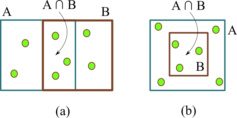
Figure 1: Two distinct situations involving two sets $A$ and $B$ that yield the same Jaccard index value of $3/7$. However, the two sets in (b) are much more compatible because $B$ is a subset of $A$ and therefore shares all its elements.

As it can be easily verified, both the situations depicted in Figure 1 lead to the same Jaccard index $\mathcal{J}=3/7$. However, the situation in (b) can be deemed to be quite distinct because, in this case, the set $B$ is completely contained in $A$ to the point of becoming a subset, i.e. $B\subset A$. In other words, all elements of $B$ are shared with the set $A$. This is not the case in the situation (a), for both sets $A$ and $B$ have elements that are not shared.

It therefore follows that it would be interesting to obtain a modification of the Jaccard index that could distinguish between these two situations. A possible approach is described as follows.

We start by considering an index capable of quantifying how much a set is relatively interior to another. Let $A$ and $B$ be any two sets. The henceforth called interiority index (also overlap index e.g. [12]) can be written as:

$$\mathcal{I}(A,B)=\frac{\left|A\cap B\right|}{\min\left\{\left|A\right|,\left|B\right|\right\}}$$ (10)

Though this index has been also known by the names of overlap or homogeneity, in this work we will adhere to the interiority term as it seems to convey more directly the concept of how much one of the sets is contained in the other.

It can be verified that $0\leq\mathcal{I}(A,B)\leq 1$. Its minimum value is observed when $A$ is completely separated from $B$, i.e. $A\cap B=0$. The maximum value is reached when any of the sets is completely contained into the other. In other words, there is no need to specify which of the two sets is being considered as being internal to the other.

By comparing Equations 10 and 10, it follows that:

$$0\leq\mathcal{I}(A,B)\leq\mathcal{J}(A,B)\leq 1$$ (11)

and it can also be verified that:

$$0\leq\mathcal{J}(A,B)\;\mathcal{H}(A,B)\leq 1$$ (12)

The verification of similarity accounted for by the Jaccard index can be conveniently combined with the interiority index simply by considering their respective product, i.e.:

$$\mathcal{C}(A,B)=\mathcal{J}(A,B)\;\mathcal{I}(A,B)$$ (13)

which is the same as:

$$\mathcal{C}(A,B)=\frac{\left|A\cap B\right|^{2}}{\left|A\cup B\right|\;\min\left\{\left|A\right|,\left|B\right|\right\}}$$ (14)

It may also interesting to take the square root of the coincidence in order to compensate for the smaller values implied when multiplying to measurements in the interval $[0,1]$. Therefore, in the present work we will adopted the coincidence indes as:

$$\mathcal{C}(A,B)=\sqrt{\mathcal{J}(A,B)\;\mathcal{I}(A,B)}$$ (15)

It is also possible, in certain situations, to dispense with the square root operation.

In some specific cases it is also possible to use these two indices separately, defining a corresponding tuple $[\mathcal{J}(A,B),\mathcal{I}(A,B)]$.

As with the Jaccard index, the coincidence index can also be generalized to virtually any mathematical structure including, we will discuss in Section 8 functions and fields in $\mathbb{R}^{N}$.

5 Weighted Discrete Elements

The Jaccard and coincidence indices can be readily adapted (e.g. [18]) to cope with cases in which the elements of sets $A$ and $B$ have been assigned respective weights corresponding to their relative importance in each specific problem.

This situation can be approached by using ordered pairs to represent each of the elements in $A\cup B$ associated to its respective weigh, i.e. $[x_{i},w(x_{i})]$. The Jaccard index then becomes:

$$\mathcal{J}_{W}(A,B)=\frac{\sum_{x_{i}\in(A\cap B)}w(x_{i})}{\sum_{y_{i}\in(A\cup B)}w(y_{i})}$$ (16)

with $0\leq\mathcal{J}_{w}(A,B)\leq 1$.

As an example, let $A=\left\{[a,2];[b,5];[c,1]\right\}$ and $B=\left\{[b,5];[e,1],[f,1]\right\}$. It follows that $A\cap B=\left\{[b,5]\right\}$.

$$\mathcal{J}_{W}(A,B)=\frac{5}{10}=\frac{1}{2}$$ (17)

Thus, in spite of in this particular example the intersection being limited to a single of the possible elements, the Jaccard index resulted relatively high as a consequence of the large weigh associated to the element $b$.

Observe that the weighted version of the Jaccard index is not the same as the Jaccard index adapted to multisets, as the latter case does not involve the sum of weights. However, it is possible to considered weighted multisets, in which case the Jaccard index becomes:

$$\mathcal{J}_{[W,M]}(A,B)=\frac{\sum_{i}{w_{i}\min\left\{a_{i},b_{i}\right\}}}{\sum_{i}{w_{i}\max\left\{a_{i},b_{i}\right\}}}$$ (18)

6 Addition-Based Multiset Jaccard Index

The multiset Jaccard index can be further generalized by taking into account the sum of the two sets $A$ and $B$ allowed by multiset theory, instead of their respective union, which leads to:

$$\mathcal{J}_{S}(A,B)=\frac{2\sum_{i=1}^{N}\min{(a_{i},b_{i})}}{\sum_{i=1}^{N}\left(a_{i}+b_{i}\right)}$$ (19)

with $0\leq\mathcal{J}_{S}(A,B)\leq 1$. Observe that other multiset operations including subtraction, complement, and intersection can also be employed to define other indices.

The interesting feature of this index is that it takes into account the situations where the multiple instances in the multisets need to be taken into account at its fullest when combining the sets.

As an example, let’s consider that $A=\left\{a,a,a,b,c,c,c\right\}$ and $B=\left\{a,a,c\right\}$. Then, we have that:

$$\mathcal{J}_{S}(A,A)=\frac{(2)(7)}{7+7}=1$$ (20)

and:

$$\mathcal{J}_{S}(A,B)=\frac{(2)(3)}{7+3}=\frac{3}{5}$$ (21)

The additive multised Jaccard index can be immediately combined with the respective interiority index to yield the addition-based multiset coincidence index.

7 Continuous Sets

The henceforth described approach holds for $\mathbb{R}^{N}$, but we shall consider the plane vector space $\mathbb{R}^{2}$. It is possible to associate sets to the points $(x,y)$ of this space in any possible manner, such as $R=\left\{(x,y)\;|\;x\text{ and }y\text{ are even}\right\}$, which is a discontinuous in $\mathbb{R}^{2}$, or $S=\left\{(x,y)\;|\;0\leq x\leq 2,-1\leq y\leq 1\right\}$, which defines a continuous region.

Though the Jaccard index can be immediately applied to any of these sets, it is of particular interest to our developments to consider sets configurations corresponding to simple connected regions of $\mathbb{R}^{2}$ such as those illustrated in Figure 2.

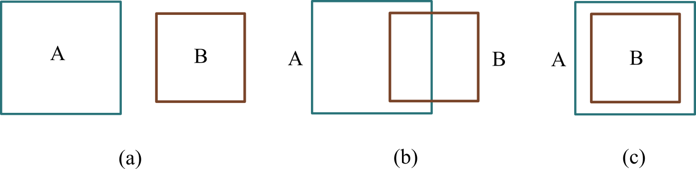
Figure 2: The three most relevant situations to be considered when comparing two sets: (a) no intersection; (b) partial interesection; (c) complete intersection.

In this case, the size of the involved sets and subsets can be conveniently represented by the respective areas, indicated as $|A|$, $|B|$, $|A\cap B|$, and $|A\cup B|$, which can be immediately used in Equation 10.

The three cases in Figure 2 correspond to the most representative situations when comparing two sets. In Figure 2(a), we have two separated sets, which results in null intersection, suggesting minimal similarity between the two sets. The situation depicted in (c) can be understood as leading to the maximum similarity that can be achieved with the sets $A$ and $B$. Figure 2(b) illustrates a frequently found situation in which there is some intersection between the sets. In this case, the similarity value would be expected to increase with the intersection area in a possibly linear manner.

The situation represented in Figure 2(b) actually incorporates the two other situations as limit cases. Consider the diagram shown in Figure 3, involving two square regions $A$ and $B$, with respective sides $a$ and $b$, $b\leq a$.

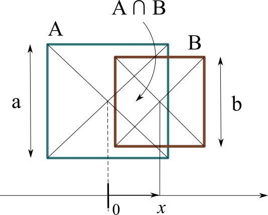
Figure 3: A construction representing all possible situations regarding the similarity of two sliding squares $A$ and $B$ with sides $a$ and $b$, respectively. Without loss of generality, we assume that $a\geq b$. Any of these situations can be specified by just two parameters: the relative position $x$ and the relative size $r=b/a$. This construction allows us to better understand the behavior of the Jaccard and other similarity indices covered in this work.

The relative position, and also the similarity, of the two sets can be completely controlled in terms of the relative position parameter $x$, with $\frac{a-b}{2}\leq x\leq\frac{a+b}{2}$. As $b$ increases, the two squares progressively separate, therefore becoming less similar.

There is only one other parameter that needs to be specified in order to completely represent the situation in Figure 3, namely the relative sizes of the two regions $r=b/a$, with $0\leq r\leq 1$.

The area of the intersection $A\cap B$ and union $A\cup B$ of the two sets can now be conveniently expressed in terms of $x$ and $b$ as:

$$|A\cap B|=(ra)\left(\frac{a}{2}-\left(x-\frac{ra}{2}\right)\right)=$$

$$\frac{1}{2}\left(a^{2}r(1+r)-2rax\right)$$ (22)

$$|A\cup B|=\frac{1}{2}\left(2a^{2}\left(1+r^{2}\right)-a^{2}r(1+r)+2rax\right)$$ (23)

We can now rewrite the Jaccard index as:

$$\mathcal{J}(A,B)=\frac{a^{2}r(1+r)-2rax}{2a^{2}\left(1+r^{2}\right)-a^{2}r(1+r)+2rax}$$ (24)

Figures 4 (a) to (c) present the Jaccard index for two rectangles, as developed above, in terms of several configurations of the parameters $x$ and $r$. Observe the yellow regions obtained for all indices, corresponing to the situations in which the smaller square is either completely insider or outside the other square.

The first row in Figure 4 concerns the Jaccard (a), interiority (b) and respectively obtained coincidence (c) indices. It can be observed that the Jaccard index values increase diagonally from top right to the lower left corner, achieving the peak $a$ at the bottom left corner in (a). The interiority index, however, varies from 0 to 1 along each vertical slice in (b), being therefore ‘degenerate’ in the mathematical sense of not implementing a bijective mapping with respect to the peak 1. Indeed, every point at the lower non-null region in (b) will correspond to maximum interiority of $1$. The coincidence index values, shown in (c) correspond to the product between the Jaccard and interiority indices, yielding a bijective association with the maximum value of 1 at the bottom right corner. Observe the respective change in the level sets shapes. Similar results hold for the addition-based Jaccard index shown in the lower row in Figure 4(d-f).

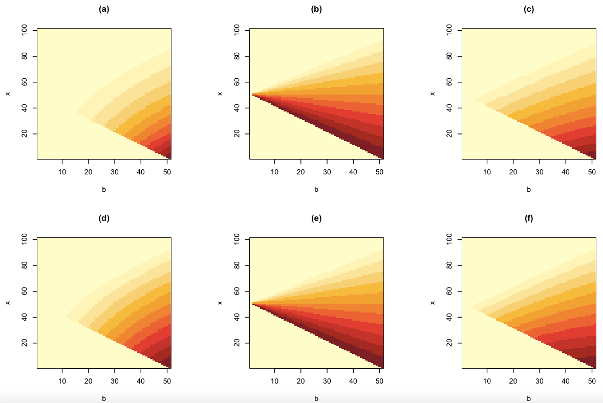
Figure 4: The Jaccard (a), interiority (b), and square root of the coincidence (c) indices obtained for the geometrical construction illustrated in Figure 3. The heat map increases from yellow to brown. The incorporation of the interiority level into the Jaccard index leads to a more comensurated distribution of the level sets. The maximum value the Jaccard and continuity indices are to be found at the lower righthand corner of the respective plots. The values of the interiority index increase linearly from the top to the bottom diagonal in (b). Along (d) to (f), we have analogous results concerning the additive multiset Jaccard index (d), the interiority (e), and square root of the additive coincidence index, the latter corresponding to the p (f). The latter index corresponds to the product of the additive multiset Jaccard and interiority indices.

The geometrical construct in Figure 3 therefore provides an interesting approach to comparing the varying results obtained in Figure 4. The rationale is as follows: as the square $B$ slides from being completely inside the square $A$, until it becomes completely outside the latter, it is reasonable to expect the similarity to decrease in a linear manner with $x$. This suggests that we can compare the several indices in Figure 4 while taking into account their respective slice along vertical slices of the scalar fields. For simplicity’s sake, we will consider five slices corresponding to $b=10,20,30,40,50$. The results are shown in Figure 5.

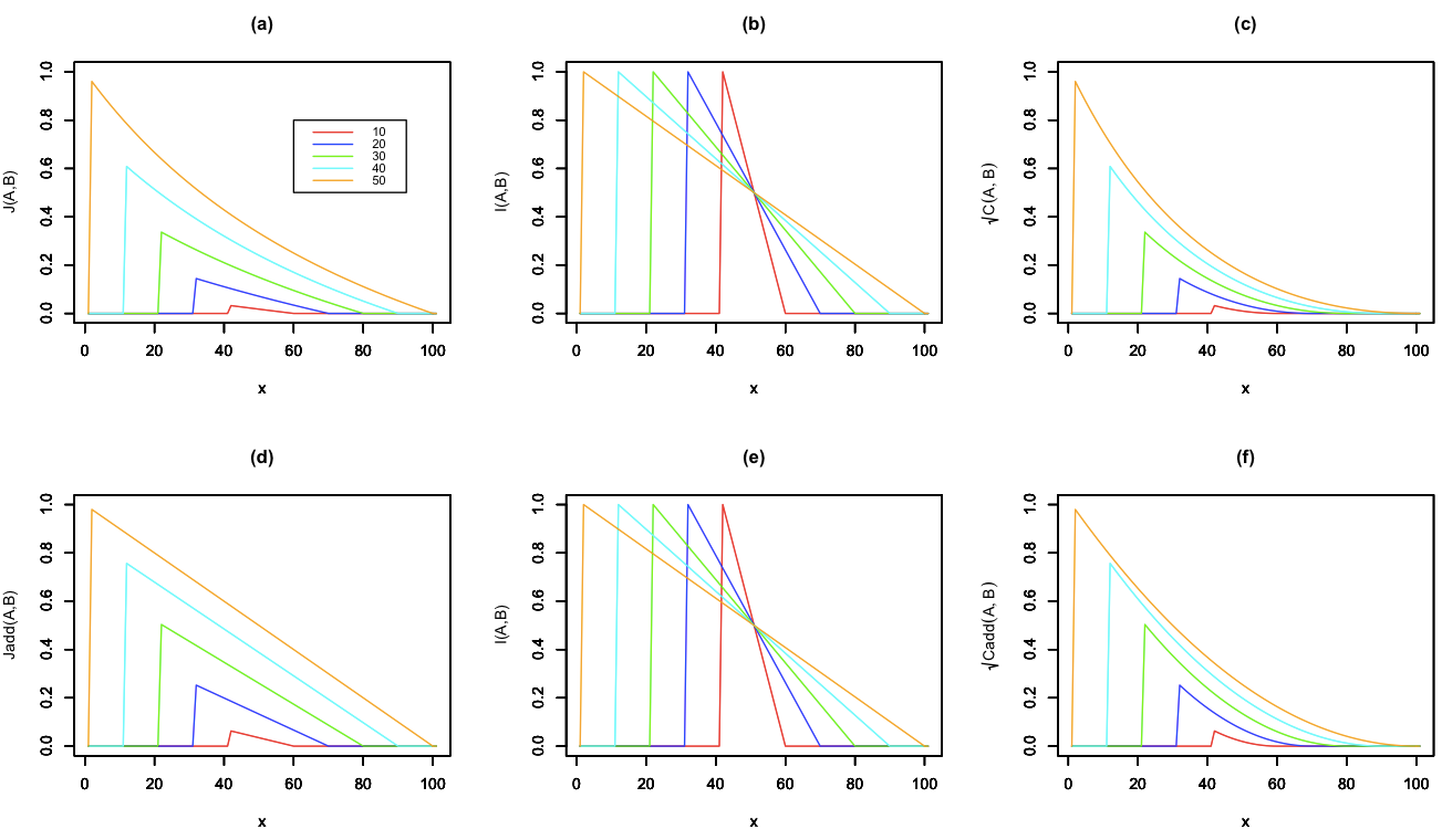
Figure 5: Five vertical slices of the respective indices in Fig. 4. Only the interiority and additive multiset Jaccard indices account for the expected linear decrease of similarity following $x$ displacements. However, the interiority is unable to take into account the relative size of the squares, which leaves only the additive multiset Jaccard as presenting a complete and linear quantification of the similarity between the two sets. The square root of the coincidence indices both penalizes the similarity when $x$ is small, with the basic coindicence index imposing the most severe test of similarity.

Among the five indices in Figure 4, only the additive multiset Jaccard index accounts for linear similarity quantification as $x$ varies also in linear manner. The interiority, as expected, is unable to consider the relative size of the sets. The coincidence indices penalize the similarity for small values of $x$ (i.e. when the slices are further away), with the basic coincidence index being more strict and selective. Also, the basic Jaccard tends to penalize these cases more intensely than the additive multised Jaccard index.

None of these indices are absolutely better than the others. It is the specific requirements of each application that should lead to a suitable choice while considering the above identified properties of each index. For instance, situations required enhanced selectivity and more strict similarity quantification may consider the adoption of any of the two described coincidence indices.

8 Continuous Densities and Scalar Fields

The developments discussed in the previous sections pave the way for considering also sets corresponding to densities, such as probability density functions, as well as completely generic functions and scalar fields. One of the main problem to be overcome here is that densities often have infinite support, meaning that they extend over infinite ranges in their respective space.

The problem of comparing two distributions is particularly important in many theoretical and applied areas, having motivated great interest and the proposal of several respective approaches (e.g. [28, 29]).

One interesting perspective that can be used to adapt the Jaccard and coincidence indices so as to allow comparison of densities is developed as follows.

We start by representing a generic continuous function in terms of a respective discretization, with resolution $\Delta x$, as illustrated in Figure 6.

Figure 6: A generic density function $p(x)$ being discretized with resolution $\Delta x$, so that it can be represented as a vector $\vec{p}=[x_{i}]\Delta x$. The integral of the original and respective discretization are assumed to be 1, so that they are both normalized as densities.

The density $p(x)$ becomes the vector $\vec{p}=[x_{i}]\Delta x$. Now, in a vector the order of the elements is all important, but it can indeed be incorporated into the multiset representation as:

$$X=\left\{[x_{1},m(x_{1});\ldots;[x_{i},m(x_{i})];\ldots[x_{n},m(x_{n})]\right\}$$ (25)

where $x_{i}$ are the elements in the respective support and $m(x_{i})$ is the multiplicity of the element $x_{i}$ generalized to take real values. In addition, we have also assumed, for simplicity’s sake, that the discretization takes place on $n$ points, which are henceforth understood as the support of both the function and the multiset. The functions transformed into their respective multisets are here called multifunctions, or mfunctions.

Now, let $m_{A}(x_{i})$ and $m_{B}(x_{i})$ correspond to the multiplicity of the elements $x_{i}$ in the two sets obtained by discretization of two density functions $p_{A}(x)$ and $p_{B}(x)$ assuming the same support. The respective multiset Jaccard can now be obtained as:

$$\mathcal{J}_{P}(A,B)=\frac{\sum_{i\in\Phi}\min(m_{A}(x_{i}),m_{B}(x_{i}))}{\sum_{j\in\Phi}\max(m_{A}(x_{j}),m_{B}(x_{j}))}$$ (26)

where $\Phi$ is the combined support of the two multisets $A$ and $B$.

This index is then capable of expressing the similarity between the two original densities up to the $x-$resolution $\Delta x$. The above reasoning extends immediately to discrete probability densities.

By making $\Delta_{x}\rightarrow 0$, we then obtain:

$$\mathcal{J}_{P}(A,B)=\frac{\int_{\Phi}\min(m_{A}(x),m_{B}(x))dx}{\int_{\Phi}\max(m_{A}(x),m_{B}(x))dx}$$ (27)

Observe that a bijective map is therefore obtained between the original density values $\left[x,p(x)\right]$ and the respective 2-tuples $\left[x_{i},(x_{i})\right]$.

As such, the Jaccard index can be understood to correspond to a functional derived fro the two functions or, perhaps more specifically, an mfunctional.

In addition to the above described limiting situation, it is also possible [2] to consider the Equation 28 directly from the real function space, without the need of taking the limit. Observe that the generalized Jaccard index as defined by equation is completely specified and valid in the space of real functions, provided the integrals exist.

The above result extends immediately to density functions on higher dimensional domains as:

$$\mathcal{J}_{P}(A,B)=\frac{\int_{\Phi}\min(m_{A}(\vec{x}),m_{B}(\vec{x}))d\vec{x}}{\int_{\Phi}\max(m_{A}(\vec{x}),m_{B}(\vec{x}))d\vec{x}}$$ (28)

Which provides a means to generalize the multiset Jaccard index to continuous or discrete scalar or vector fields for any number of random variables.

As an example of the generalization of multisets to real values, let’s consider the two density functions $X_{A}$ and $X_{B}$ depicted in Figure 7(a).

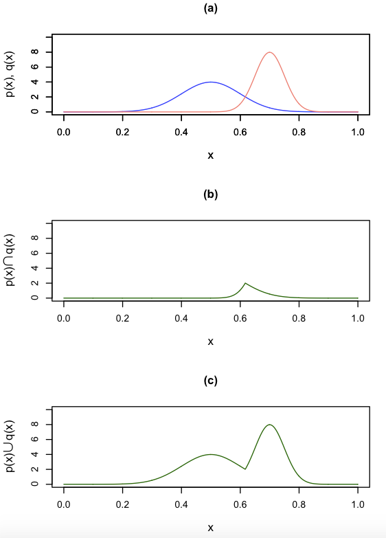
Figure 7: Two probability density functions $p(x)$ and $q(x)$ (a), with respective intersection and union as shown in (b) and (c). This situation yields a Jaccard index equal to 0.41. The maximum value 1 is obtained whenever the two densities are identical.

The respective intersection $X_{A}\cap X_{B}$ and union $X_{A}\cup X_{B}$ of these two densities, obtained by using the minimum and maximum operation between the elements of pair of values, are presented in Figures 7(a) and (b), respectively. The Jaccard index, obtained by dividing the area of the intersection curve by the area of the union, yielded the value 0.09257.

It is also interesting to observe that the comparison of two densities can be represented as a scatterplot, with the two density functions defining a parametric curve. This is illustrated in Figure 8. The closest the set of points covered by the respectively obtained parametric curve are to the identity line (in salmon), the higher the similarity index between the two densities will be. This construction can be immediately extended to generic functions.

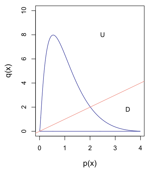
Figure 8: The two probability densities $p(x)$ and $q(x)$ in Figure 7 shown as a parametric curve in the respective scatterplot. In case of discrete densities, they can be represented in terms of parametric curves related to the joint observations. Continuous densities can be represented in a similar manner. The identity line, shown in salmon, partitions the scatterplot space into the two regions $U$ and $D$.

The Jaccard index can be also adapted to quantify the separation of two groups of points, or clusters, which can be understood as a discrete or continuous scalar field. The basic idea here would be to represent each of the clusters in terms of the joint probability density and then apply the Jaccard index over them by considering the densities as the respective multiplicity of every element. This method can be applied to any number of involved features.

Though we have so far considered both $X_{A}(\vec{x})$ and $X_{B}(\vec{x})$ to correspond to non-negative scalar fields with hypervolume 1, it is actually possible to employ the Jaccard and coincidence indices to quantify the similarity between any two scalar mfunctions or mfields $\phi_{A}(\vec{x})$ and $\phi_{B}(\vec{x})$ sharing the same domain, even in presence of negative multiplicities.

The extension of similarity indices to negative values has been previously approached in [13, 30, 31]. A respective possible manner to adapt the Jaccard index to negative multiplicities in a two-dimensional space is as follows. In case the pair of points $[m(X_{A}),m(X_{B})]$ is in the first quadrant, the minimum and maximum between the two multiplicities are accumulated into the intersection and union integral, respectively. It the point is in the third quadrant, both coordinates have their signal inverted and the respective minimum and maximum are accumulated.

Otherwise, if the point belongs to the II or IV quadrant, the point $[m(X_{A}),m(X_{B})]$ is mirrored into the opposite quadrant respectively to the vertical axis, and it is the negative of the minimum between the multiplicities that is then accumulated into the intersection integral (to compensate for the reflection), while the union is taken with positive sign, and the resulting accumulated intersection and union are then used in Equation 28 to obtain the respective Jaccard index.

Figure 9: Jaccard for mfunctions with negative multiplicity. Points in the II and IV quadrants are reflected with respect to the vertical axes, and their intersection (minimum values) and union (maximum values) enter with negative values in the accumulated intersection and union.

For instance, let’s calculate the multisets Jaccard index for the functions $f(x)=cos(\theta)$ and $g(x)=sin(\theta)$ for a complete period $0\leq\theta\leq 2\pi$, as illustrated in Figure 10.

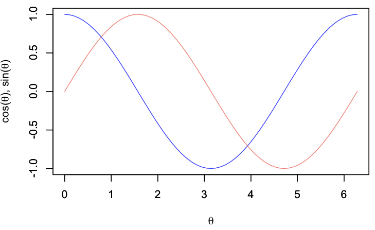
(a)

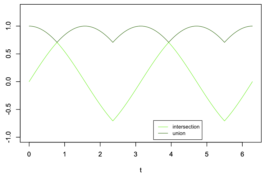
(b)

Figure 10: The Jaccard index calculated for a cosine and a sine function. The mfunctions are shown in (a), and the respective interesection and union mfunctions are shown in (b). The obtained Jaccard index was equal to 0. Indices of 1 and -1 will be obtained in case $g(x)=cos(t)$ and $g(x)=-cos(t)$, respectively.

This operation, which has been found to correspond to the intersection of real multisets with possibly negative values [11, 32], can be summarized as:

$$f(x)\sqcap g(x)=\int_{S}s_{f}s_{g}\min(s_{f}f(x),s_{g}g(x))dx$$ (29)

where $S$ is the combined support of $f(x)$ and $g(x)$.

From which, the multiset convolution [11] (mconvolution) of two functions can be derived:

$$f(x)\Box g(x)[y]=\int_{S}\frac{f(x)\sqcap g(x-y)}{f(x)\tilde{\sqcup}g(x-y)}dx$$ (30)

where $f(x)\tilde{\sqcup}g(x-y)$ corresponds to the absolute value union of generalized multisets [32]:

$$f(x)\tilde{\sqcup}g(x)=\int_{S}s_{f}s_{g}\min(s_{f}f(x),s_{g}g(x))dx$$ (31)

Equation 30 presents a direct analogy to the multiset Jaccard index. The other generalizations of the Jaccard index can be readily employed in the above expressions in order to cater for less or more strict similarity quantification.

Preliminary results have shown that the multiset convolution provides, in general, sharper and more selective peaks and smaller sidelobes than the standard correlation [11, 33].

A further example of the Jaccard index adapted to multidimensional scalar fields, namely a gray level image, also incorporating the respective scatterplot representation of the paired multiplicities is provided in Figure 11.

(a)

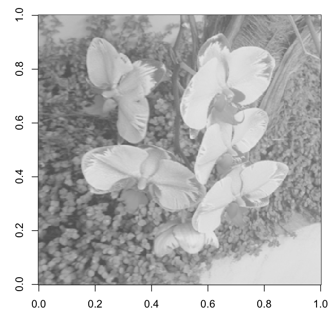
(b)

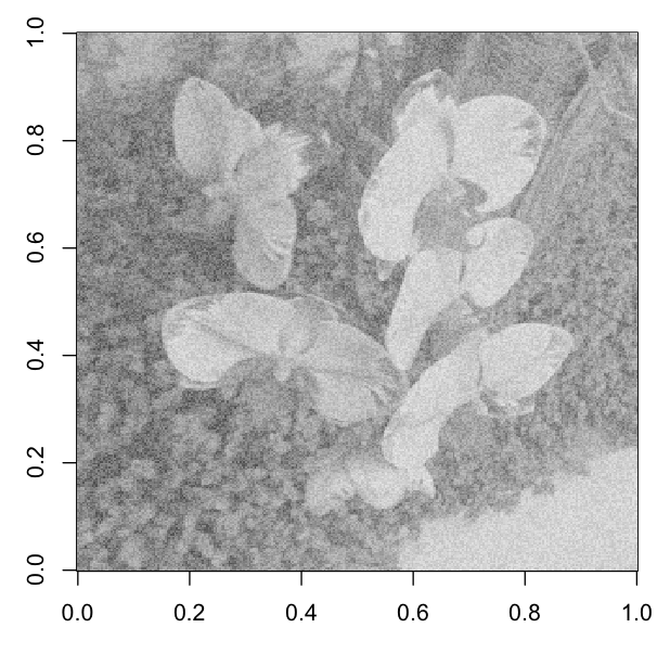
(c)

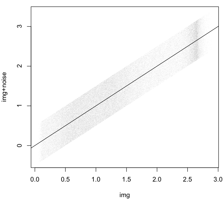
Figure 11: A gray level image of flowers $img[x,y]$ (a) was mixed with random noise uniformly distributed between $-0.5$ and $0.5$, resulting in the noisy image $img[x,y]+\xi[x,y]$ shown in (b). The resulting scatterplot is depicted in (c), including the identity line defining the two regions for calculation of the scalar field intersection and union, from which a respective Jaccard index of $\mathcal{J}(img,img+\xi)=0.83$ was obtained, reflecting a relatively high similarity between the two scalar fields.

9 Joint Variations

Joint variation are often taken in a normalized manner as when using the Pearson correlation coefficient. More specifically, we have that this coefficient can be understood as corresponding to the variance provided the samples of the two sets have been first standardized. By standardization it is henceforth understood that, given a random variable $X$, we apply the following random variable transformation:

$$\tilde{X}=\frac{X-\mu_{X}}{\sigma_{X}}$$ (32)

This standardization has the effect of normalizing the dispersions of a random variables, so that the its variance becomes 1 while the average is 0. It can also be verified that a standardized random variable will present most of its observations within the interval $[-2,2]$.

In the case of a set of $N$ observations of two standardized random variables, the Pearson correlation coefficient becomes:

$$\mathcal{P}(X,Y)=\frac{1}{N}\sum_{i,j=1}^{N}{[\tilde{X}_{i}][\tilde{Y}_{i}]}$$ (33)

When two standardized random variables $\tilde{X}$ and $\tilde{Y}$ are taken jointly, they define a scatterplot providing a useful illustration about the interrelationship between the two considered values. This scatterplot can be immediately understood as corresponding to a sampling of the joint probability density of the two random variables, which may be kernel expanded to obtain an estimation of the respective counterpart.

The quantification of joint variation by a L1-based operatoron possibly negative values [31] has been previously addressed [34].

It constitutes an interesting issue to consider joint variation quantification based on the Jaccard and coincidence indices. In order to illustrate the possibility to quantify the joint variation of observations in a scallterplot (or, actually, joint densities), we consider the situation in Figure 12, which shows several scatterplots drawn from normal densities with increasing correlation.

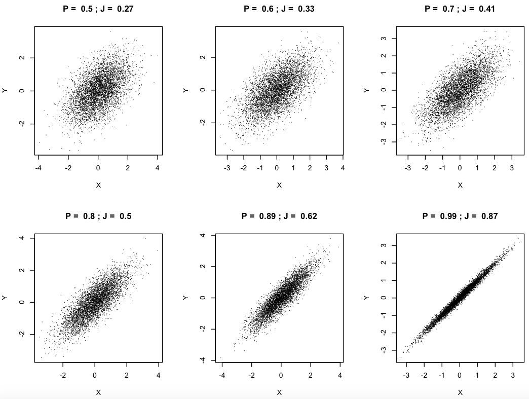
Figure 12: Comparision of the Pearson correlation coefficient and the multiset Jaccard index for negative multiplicities with respect to several distribution of points with increasing correlation. Interestingly, the Jaccard index seems to provide a more gradual quantification of the joint variations that is probably more compatible with our perception. At the same time, the respective Pearson correlation coefficients tend to saturate as the correlation increases.

10 Multiple Sets

We have so far considered indices applied to two sets or entities. There are two basic ways in which more sets can be taken into account. The first one consists of simply understanding that each of the two sets $A$ and $B$ are obtained by set operation combinations among several other sets.

For instance, in case we are interested in $A=(C\cap D)\cup E-F$ and $B=C\cup G$, we can write:

$$A=f(C,D,E,F)$$

$$B=f(C,G)$$

and then apply the Jaccard or coincidence indices.

Observe that there is absolute no restriction on these functions, except that they are not both empty sets.

The Jaccard index for the example above can be expressed as:

$$\mathcal{J}(A(C,D,E,F),B(C,G))=\frac{\left|A(C,D,E,F)\cap B(C,G)\right|}{\left|A(C,D,E,F)\cup B(C,G)\right|}$$

Therefore, a vast range of possible combinations of diverse sets become possible, but they will ultimately always lead to two resulting sets $A$ and $B$ to be compared by the Jaccard or coincidence indices.

There is another interesting possibility to take into account more than 2 sets, and this corresponds to extending the Jaccard index, for instance in the case involving 3 sets, as:

$$\mathcal{J}_{3}(A,B,C)=\frac{\left|A\cap B\cap C\right|}{\left|A\cup B\cup C\right|}$$

with $0\leq\mathcal{J}(A,B,C)\leq 1$. This concept can be immediately extended to any number $N_{S}$ of sets.

The extension of the interiority index becomes:

$$\mathcal{I}_{[3,1]}(A,B,C)=\frac{\left|A\cap B\cap C\right|}{\min\left\{\left|A\right|,\left|B\right|,\left|C\right|\right\}}$$

It can be verified that this extended interiority index now quantifies how much the smallest of the sets is contained in the overall intersection. However, it does not take into account how the intermediate size set relates to the mutual intersection. This can be accomplished by introducing a second interiority index as:

$$\mathcal{I}_{[3,2]}(A,B,C)=\frac{\left|A\cap B\cap C\right|}{\left|X\right|}$$

where $X$ is the set with the second smallest cardinality.

The two obtained interiority indices can then be combined into a single respective index as:

$$\mathcal{I}_{3}(A,B,C)=\mathcal{I}_{[3,1]}(A,B,C)\;\mathcal{I}_{[3,2]}(A,B,C)$$

with $0\leq\mathcal{I}_{3}(A,B,C)\leq 1$.

We can now define the coincidence index extended to three sets as:

$$\mathcal{C}_{3}(A,B,C)=\mathcal{I}_{3}(A,B,C)\;\mathcal{J}_{3}(A,B,C)$$

A similar development applies to more than 3 sets.

The consideration of more than 2 sets in similarity index suggests other possible extensions of the Jaccard and coincidence indices. For instance, it becomes interesting not only to quantify the overall similarity between 3 sets, but also to develop indices capable of reflecting how these three sets are connected one another. Consider the situation depicted in Figure 13.

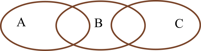
Figure 13: Three sets $A$, $B$ and $C$ characterized by sequential, or chained intersections. In the suggested approach, $B$ is taken as a candidate reference for intermediating the other two sets through a chaining relationship.

This situation suggests that set $B$ intermediates the connection between the sets $C$ follows and $A$, therefore establishing a chaining relationship. The Jaccard index with 2 sets cannot cope directly with this situation.

A possible index involving three sets that can quantify the chaining between 3 sets is:

$$\mathcal{X}(A,B,C)=\mathcal{J}(B,(A\cap B)\cup(B\cap C))\;\left[1-\mathcal{J}(A,C)\right]$$

As an example, let’s consider:

$$A=\left\{a,b,c,d,e,f,g\right\};$$

$$B=\left\{e,f,g,h,i,j,k\right\};$$

$$C=\left\{i,j,k,l,m,n,o\right\}$$

It folows that:

$$A\cap B=\left\{e,f,g\right\};$$

$$A\cap C=\left\{\right\};$$

$$B\cap C=\left\{i,j,k\right\};$$

$$A\cup C=\left\{a,b,c,d,e,f,g,i,j,k,l,m,n,o\right\};$$

$$(A\cap B)\cup(B\cap C)=\left\{e,f,g,i,j,k\right\};$$

$$B\cap[(A\cap B)\cup(B\cap C)]=\left\{e,f,g,i,j,k\right\}$$

$$B\cup[(A\cap B)\cup(B\cap C)]=\left\{e,f,g,h,i,j,k\right\}$$

So, we have that:

$$\mathcal{J}(B,(A\cap B)\cup(B\cap C))=$$

$$=\frac{\left|B\cap[(A\cap B)\cup(B\cap C)]\right|}{\left|B\cup[(A\cap B)\cup(B\cap C)]\right|}=\frac{6}{7}$$ (34)

and:

$$\mathcal{J}(B,C)=\frac{|A\cap C|}{|A\cup C|}=\frac{0}{14}=0$$ (35)

From which we obtain the chaining index value of:

$$\mathcal{X}(A,B,C)=$$

$$=\mathcal{J}(B,(A\cap B)\cup(B\cap C))\;\left[1-\mathcal{J}(A,C)\right]=$$

$$=\frac{6}{7}\left[1-0\right]=\frac{6}{7}$$

which provides an interesting indication of the chaining between the sets $A$, $B$, and $C$. Observe that the above described approach assumes that set $B$ has been adopted as a reference for implementing the chaining between $A$ and $C$. More generic situations can be addressed by considering successive pairwise combinations.

It should be observe that it is possible that one of the intersections betwen $B$ and $A$ or $C$ is large enough to bias the above index. In these situations, it is possible to incorporate an additional index specifying a minimum overlap between both $A$ and $B$ as well as $B$ and $C$.

Several other analogous chaining indices involving 3 or more sets or other structures are possible, leading to complementary properties.

11 The Jaccard and Coincidence Indices in Modeling

By allowing several types of mathematical structures to have their relationships to be quantified in terms of respective indices, it becomes possible to objective and quantitatively address a wide range of theoretical and practical problems, while also catering for the consideration of stochasticity.

In addition, the several indices discussed and suggested in this work represent a valuable resource while developing models (e.g. [35]) through the combination of datasets as described in [1].

Then, we have several additional possibilities of applying these indices. For instance, a new dataset can be compared to those already modeled by using the similarity indices. Also of particular interest is to identify which combinations, through set operations, between the existing datasets associated to models are more likely to account for other datasets of interest, therefore providing insights about how respective models can be identified, related, or developed.

The discussed indices are also interesting from the perspective of characterizing, developing, validating and applying pattern recognition and deep learning approaches [36, 37, 38].

12 Concluding Remarks

Relationships between the several important mathematical structures — including sets, functions, vectors, densities, and graphs — are critically important in virtually all areas where mathematics is employed. Given its interesting features, the Jaccard index has been extensively employed in a large range of scientific and technological situations. Also as a consequence of its potential, the Jaccard index has been generalized in several manners.

The present work aimed at generalizing further the Jaccard index. One of the first discussed possibilities consisted in using the interiority index, capable of quantifying how much a set is contained into another, as means to complement a identified limitation of the Jaccard index in taking into account the interiority of one set into the other . This index was then combined with the Jaccard index to yield the coincidence index, which is believed to provide a more strict and selective quantification of the similarity between sets. The possibility to adopt the sum of multisets instead of the union was also addressed, with promising results for the situations where the multiplicity of the elements have to be fully taken into in account.

The possibility to apply the Jaccard and coincidence indices on continuous sets was then addressed by considering the areas of the involved regions in place of the number of set elements. This adaptation of the Jaccard index allowed the consideration of density fields and functions, which was approached by using the Jaccard index for multisets. The potential of this generalization of the Jaccard index was then briefly illustrated with respect to probability density functions as well as in a comparison between the cosine and sine functions, which are not normalized and can take negative values, as well as a real-world image and a respective noise version.

The intrinsic relationship between similarity indices and statistical quantifications of joint variation between random variables was approached subsequently, and it has been argued that both the Pearson correlation coefficient can be used to compare two density functions, but also that a respective adaptation of the Jaccard and coincidence indices can also be used for that finality. We also discussed the interesting possibility to visualize the action of the Jaccard and coincidence indices with respect to the division of the data into two regions defined by the identity line in the scatterplot distribution.

The also interesting situation of similarity and other indices considering three or more sets was then discussed, identifying the possibility to consider the two sets involved in the basic Jaccard and coincidence index as corresponding to the result of set operation combinations between any number of other sets. Another important extension was considered with respect to taking into account more than 2 sets as arguments for the similarity indices, which was illustrated in terms of a suggested index to quantify the chaining between three sets.

Several are the further possible works motivated by the concepts and methods reported and suggested in this work, a more complete list of which would be particularly extensive. Some of the possibilities include comparing the described indices with other indicators of similarity, the identification of other types of relationships that can be quantified when considering 3 or more sets and analogue generalizations of other interesting indices, as well as extending the described indices to other mathematical structures.

In addition, as observed in Section 11, similarity and other indices such as those addressed here provide valuable means for developing and evaluating models of data as well as for several pattern recognition and deep learning tasks.

Acknowledgments.

Luciano da F. Costa thanks CNPq (grant no. 307085/2018-0) and FAPESP (grant 15/22308-2).

References

- [1] L. da F. Costa. An ample approach to modeling. Researchgate, 2019. https://www.researchgate.net/publication/355056285_An_Ample_Approach_to_Data_and_Modeling. [Online; accessed 10-Oct-2021.].
- [2] L. da F. Costa. Analogies between boolean algebra, set theory and function spaces. https://www.researchgate.net/publication/355680272_Analogies_Between_Boolean_Algebra_Set_Theory_and_Function_Spaces, 2021. [Online; accessed 21-Oct-2021].
- [3] B. K. Samanthula and W. Jiang. Secure multiset intersection cardinality and its application to jaccard coefficient. IEEE Transactions on Dependable and Secure Computing, 13(5):591–604, 1989.
- [4] D. Bacciu, A. Micheli, and A. Sperduti. Generative kernels for tree-structured data. IEEE Transactions on Neural Networks and Learning Systems, 29(10):4932–4946, 2018.
- [5] J. Hein. Discrete Mathematics. Jones & Bartlett Pub., 2003.
- [6] D. E. Knuth. The Art of Computing. Addison Wesley, 1998.
- [7] W. D. Blizard. Multiset theory. Notre Dame Journal of Formal Logic, 30:36—66, 1989.
- [8] W. D. Blizard. The development of multiset theory. Modern Logic, 4:319–352, 1991.
- [9] P. M. Mahalakshmi and P. Thangavelu. Properties of multisets. International Journal of Innovative Technology and Exploring Engineering, 8:1–4, 2019.
- [10] D. Singh, M. Ibrahim, T. Yohana, and J. N. Singh. Complementation in multiset theory. International Mathematical Forum, 38:1877–1884, 2011.
- [11] L. da F. Costa. Multisets. https://www.researchgate.net/publication/355437006_Multisets, 2021. [Online; accessed 21-Aug-2021].
- [12] M. K. Vijaymeena and K. Kavitha. A survey on similarity measures in text mining. Machine Learning and Applications, 3(1):19–28, 2016.
- [13] B. Mirkin. Mathematical Classification and Clustering. Kluwer Academic Publisher, Dordrecth, 1996.
- [14] R. A. Jarvisand E. A. Patrick. Clustering using a similarity measure based on shared near neighbors. IEEE Transactions on Computers, C-22:1025–1034, 1973.
- [15] R. A. Miranda-Quintana, D. Bajusz, A. Rácz, and K. Héberger. Extended similarity indices: the benefits of comparing more than two objects simultaneously. part 1: Theory and characteristics. J. Cheminformatics, 13, 2021.
- [16] H. Wolda. Similarity indices, sample size and diversity. Oecologia, 50:296–302, 1981.
- [17] M. Brusco, J. D. Cradit, and D. Steinley. A comparison of 71 binary similarity coefficients: The effect of base rates. PLOS One, 16(4):e0247751, 2021.
- [18] Wikipedia. Jaccard index. https://en.wikipedia.org/wiki/Jaccard_index. [Online; accessed 10-Oct-2021].
- [19] P. Jaccard. Distribution de la flore alpine dans le bassin des dranses et dans quelques régions voisines. Bulletin de la Société vaudoise des sciences naturelles, 37:241–272, 1901.
- [20] Fr-Academic.com. Paul jaccard. Fr-Academic.com, 2021. https://fr-academic.com/dic.nsf/frwiki/1306378. [Online; accessed 10-Nov-2021.].
- [21] T. T. Tanimoto. An elementary mathematical theory of classification and prediction. Internal IBM Technical Report, 1958.
- [22] Y. Yuan, M. Chao, and Y.-C. Lo. Automatic skin lesion segmentation using deep fully convolutional networks with jaccard distance. IEEE Transactions on Medical Imaging, 36(9):1876–1886, 2017.
- [23] L. Hamers, Y. Hemeryck, G. Herweyers, M. Janssen, H. Ketters, H. Rousseau, and A. Vanhoutte. Similarity measures in scientometric research: The jaccard index versus salton’s cosine formula. Information Processing and Management, 25(3):315–318, 1989.
- [24] L. Leydesdorff. On the normalization and visualization of author co-citation data: Salton’s cosine versus the jaccard index. Journal of the American Society for Information Science and Technology, 59(1):77–85, 2008.
- [25] S. Park and D.-Y. Kim. Assessing language discrepancies between travelers and online travel recommendation systems: Application of the jaccard distance score to web data mining. Technological Forecasting and Social Change, 123:381–388, 2017.
- [26] M. Kurz. Paul jaccard. Dictionnaire Historique de la Suisse – DHS, 2019. https://hls-dhs-dss.ch/fr/articles/031406/2005-09-01/. [Online; accessed 10-Nov-2021.].
- [27] P. Jaccard. Étude comparative de la distribution florale dans une portion des alpes et des jura. Bulletin de la Société vaudoise des sciences naturelles, 37:547–549, 1901.
- [28] S.-H. Cha. Comprehensive survey on distance/similarity measures between probability density functions. Intl. J. Math. Models and Meths. in Appl. Sci., 1(4):300–307, 2007.
- [29] J. D. Loudin and H. E Miettinen. A multivariate method for comparing n-dimensional distributions. In PHYSTAT2003, SLAC, 2003.
- [30] C. E. Akbas, A. Bozkurt, M. T. Arslan, H. Aslanoglu, and A. E. Cetin. L1 norm based multiplication-free cosine similiarity measures for big data analysis. In IEEE Computational Intelligence for Multimedia Understanding (IWCIM), France, Nov. 2014.
- [31] C. E. Akbas, A. Bozkurt, A. E. Cetin, R. Cetin-Atalay, and A. Uner. Multiplication-free neural networks. In Signal Processing and Communications Applications Conference (SIU), Malatya, Turkey, May. 2015.
- [32] L. da F. Costa. Generalized multiset operations. https://www.researchgate.net/profile/Luciano-Da-F-Costa, 2021. [Online; accessed 10-Nov-2021].
- [33] L. da F. Costa. Comparing cross correlation-based similarities. https://www.researchgate.net/publication/355546016_Comparing_Cross_Correlation-Based_Similarities, 2021. [Online; accessed 21-Oct-2021].
- [34] H. Pan, D Badawi, E. Koyuncu, and A. E. Cetin. Robust principal component analysis using a novel kernel related with the l1-norm. https://arxiv.org/abs/2105.11634, 2021. [Online; accessed 16-Nov-2021].
- [35] L. da F. Costa. Modeling: The human approach to science. Researchgate, 2019. https://www.researchgate.net/publication/333389500_Modeling_The_Human_Approach_to_Science_CDT-8. [Online; accessed 1-Oct-2020.].
- [36] G. E. Hinton. Training products of experts by mini-mizing contrastive divergence. Neural computation, 14(8):1771–1800, 2002.
- [37] J. Schmidhuber. Deep learning in neural networks:an overview. Neural networks, 61:85–117, 2015.
- [38] H. F. de Arruda, A. Benatti, C. H. Comin, and L. da F. Costa. Learning deep learning. Researchgate, 2019. https://www.researchgate.net/publication/335798012_Learning_Deep_Learning_CDT-15. [Online; accessed 22-Dec-2019.].