The Two Cultures for Prevalence Mapping: Small Area Estimation and Spatial Statistics

Abstract

The emerging need for subnational estimation of demographic and health indicators in low- and middle-income countries (LMICs) is driving a move from design-based area-level approaches to unit-level methods. The latter are model-based and overcome data sparsity by borrowing strength across covariates and space and can, in principle, be leveraged to create fine-scale pixel level maps based on household surveys. However, typical implementations of the model-based approaches do not fully acknowledge the complex survey design, and do not enjoy the theoretical consistency of design-based approaches. We describe how spatial methods are currently used for prevalence mapping in the context of LMICs, highlight the key challenges that need to be overcome, and propose a new approach, which is methodologically closer in spirit to small area estimation. The main discussion points are demonstrated through a case study of vaccination coverage in Nigeria based on 2018 Demographic and Health Surveys (DHS) data. We discuss our key findings both generally and with an emphasis on the implications for popular approaches undertaken by industrial producers of subnational prevalence estimates.

1 Introduction

Accurate tracking of the Sustainable Development Goals (SDGs) set forth in General Assembly of the United Nations, (2015) requires the estimation of a range of demographic and health indicators across all countries of the world. We focus on indicators that can be expressed as proportions of individuals that are in the binary states of interest. Examples include the neonatal mortality rate, vaccination coverage, female attainment of specific years of education and percentage below the poverty line. In addition to monitoring attainment of targets, subnational estimates of such indicators are a key aid to designing effective health and economic policies and ensuring that no one is left behind in implementing the United Nations 2030 development agenda (UN System Chief Executives Board for Coordination,, 2017).

The subnational areas of interest are the first administrative level (admin1) and the second administrative level (admin2), which are nested partitions of the national level (admin0) geography. Admin2 is the level at which many health policy decisions are made (Hosseinpoor et al.,, 2016). In many low- and middle-income countries (LMICs), a reliable data source is provided by household surveys such as the Demographic and Health Surveys (DHS) and the Multiple Indicator Cluster Surveys (MICS). Both conduct stratified two-stage cluster sampling. For the purposes of sampling, a country consists of geographical areas that are crossed with an urban/rural indicator to produce stata. Within these strata are small enumeration areas (EAs), also called clusters, that consist of collections of households. A survey is conducted by sampling a specific number of clusters in each stratum, and sampling a specific number of households within each selected cluster. This means that each household has an inclusion probability that describes the a priori probability that it will be included in the sample. Recent survey samples are point-referenced. Small area estimation (SAE) is the endeavor of, “producing reliable estimates of parameters of interest … for subpopulations (domains or areas) of a finite population for which samples of inadequate size or no samples are available” (Rao and Molina, 2015, p. xxiii). In the terminology of SAE, one may consider area-level and unit-level approaches, with the units corresponding to clusters in our LMIC context (and it is the geographical location of the cluster that gives the spatial ‘point’).

DHS surveys are typically powered to admin1, i.e., they collect sufficient samples for reliable estimation of key indicators for admin1 areas. Hence, at admin1, it is natural to report weighted estimates, which use information on the survey design and the inclusion probabilities. In the language of SAE (Rao and Molina,, 2015), a weighted estimate is an example of a direct estimate that only uses information on the response variable for the specific area. By contrast, indirect estimates allow borrowing of response information from other areas. The seminal Fay and Herriot, (1979) model provides an early example of a hierarchical indirect area-level model, in which a (possibly transformed) weighted estimate is taken as response. The original model included area-level covariates and normal random effects, assumed to be independent across areas. Many extensions of the Fay-Herriot model, including the use of discrete spatial models and space-time generalizations have been proposed (You and Zhou,, 2011; Marhuenda et al.,, 2013; Mercer et al.,, 2015; Watjou et al.,, 2017). These SAE models are called area-level models because aggregated response variables are modeled. A key feature is that the survey design is acknowledged through the use of weighted estimators and their associated variances.

Unfortunately, if the target areas contain few samples, it is not possible to obtain a weighted estimate and accompanying variance. To deal with this, a more flexible but assumption-laden approach is provided by unit-level models that are specified at the level of the cluster and include area-level random effects (Battese et al.,, 1988). The challenges with unit-level models are that: (i) they require model terms that explicitly acknowledge the design, and (ii) area-level estimates are not directly available without an aggregation procedure. With respect to (i), fixed effects are typically included to account for stratification, and independent random effects are included to account for the clustering aspect. In many settings, it is common practice to include covariates at either the area- or the unit-level. However, as regards (ii), in the context of LMICs, including cluster- or individual-specific covariates is challenging since aggregation to produce area-level estimates requires reliable covariate values for the unobserved units, and these may not be available (or be only available through modeling). More details and further variations of area-level and unit-level SAE models can be found in Rao and Molina, (2015).

Unit-level spatial models that include variation over continuous space, i.e., geostatistical models, have been used to produce pixel maps (e.g., at the $1\times 1\,\text{km}$ or $5\times 5\,\text{km}$ level) for a range of indicators (Diggle and Giorgi,, 2016; Golding et al.,, 2017; Utazi et al.,, 2020; Local Burden of Disease Vaccine Coverage Collaborators and others,, 2021). To facilitate the comparison of such methods with SAE approaches, we make a distinction between prevalence, which is the empirical proportion of the finite population within the administrative area who are in the binary state, and risk, which is the analogous proportion of a hypothetical infinite population. SAE approaches perform prevalence mapping, i.e., the empirical proportions for areas are estimated and mapped, while most current endeavors using spatial statistics methods approximate prevalences through risk mapping, where areal risk estimates are extracted based on a geostatistical model.

More specifically, a geostatistical model is expressed in terms of an unobservable spatial risk surface that exists independently of the finite population. Each point-referenced observation is viewed as the result of a group of individuals being exposed to the risk at the given location. The risk surfaces are described in terms of Gaussian random fields and spatial covariates, and may borrow strength across space and covariates. The advantage of defining models in continuous space is that estimates of risk can be made at the pixel level. However, aggregating these risk surfaces to areal risk estimates poses a major challenge since auxiliary population information is needed and the geostatistical models use non-linear link functions. Further, auxiliary information such as fine-scale rasters of population density are modelled quantities with uncertainty, but it is not clear how to propogate this uncertainty into the aggregate estimates.

For linear models, both the SAE and the spatial statistics literature are interested in optimal linear predictors. The former in the context of finite population summaries such as means and totals, and the latter in terms of point predictions or averages over areas. However, optimal predictions at a given spatial resolution, say pixel-level or admin2, combined with an aggregation procedure, which uses imprecise and inaccurate knowledge about the population, are not guaranteed to result in optimal predictions at coarser levels such as admin1 or admin0. In this paper, we formally evaluate the accuracy and precision of different approaches with the aim being to provide a recommended workflow for prevalence mapping.

With respect to the title of this paper, we take SAE methods to correspond to area-level models in which design-based inference is carried out, while spatial statistics methods correspond to unit-level model-based inference with geostatistical spatial models and aggregation required to produce areal estimates. The area-level approach is explicitly linked to the data collection process and directly considers the discrete areas of interest. The unit-level models that are typically used in a LMIC context do not adjust for the design, with the implicit assumption that the sampling procedure is non-informative under the specified model. Our approach in data sparse situations is to marry the two approaches. We take from SAE the focus on adjustment for the design (as far as is possible given the available data) – we use unit-level (sampling) models but with area-level spatial random effects that are specified at the target areal level of inference; we also focus greater attention on the aggregation step than is typically the case. As is more common in spatial statistics that in SAE, we take a fully-Bayesian approach, with efficient implementation through integrated nested Laplace approximations (INLA) as described in Rue et al., (2009). Through the case study, we emphasize that estimation at different administrative levels may call for different approaches. Specifically, we consider spatial estimation of vaccination coverage for admin1 and admin2 areas in Nigeria in 2018. We compare the new approach, area-level SAE approaches and standard geostatistical models, through quantitative model validation based on cross-validation of cluster-level predictions and hold-out-area validation of admin1 estimates. Figures 1(a) and 1(b) show the admin1 areas and admin2 areas, respectively.

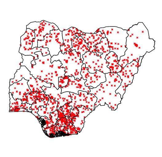
(a) Admin1.

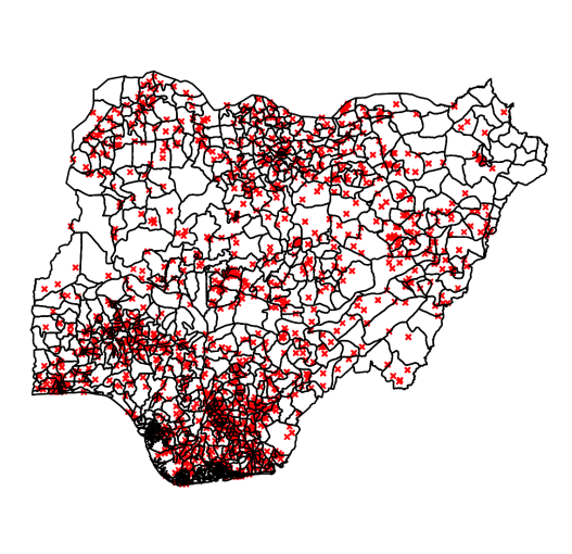
(b) Admin2.

Figure 1: Maps of Nigeria showing 1(a) the 37 admin1 areas, and 1(b) the 774 admin2 areas. The crosses show the locations of the 1389 sampled clusters.

The outline of the paper is as follows. In Section 2, we describe the background to our motivating case study, including a discussion of finite populations and complex surveys. Then, in Section 3, we describe the core ideas of design-based inference and the area-level modeling of weighted estimates including spatial and auxiliary variable smoothing. This is followed by a discussion of unit-level models, again considering spatial and auxiliary variable smoothing, along with the key aggregation step, in Section 4. In Section 5, our proposed model is described in detail. We present the most important results from the Nigeria case study in Section 6, and the paper ends with a discussion in Section 7. Supplementary model details and additional results are relegated to Appendix A, and data and code are available at https://github.com/gafuglstad/prevalence-mapping.

2 Household survey data

2.1 Finite populations and target parameters

In design-based inference, we consider a finite target population in a study area that consists of $N>0$ observation units. In the motivating example, these units are children aged 12–23 months at a given point in time. The target population can be represented as the set of indices $U=\{1,2,\ldots,N\}$ where observation unit $i$ has an associated value $y_{i}\in\{0,1\}$ for $i\in U$. These values are deterministic and unknown. When a country is divided into $A$ administrative areas, these areas partition the population $U$ into $A$ disjoint subpopulations, $U=U_{1}\cup U_{2}\cup\cdots\cup U_{A}$, where $U_{a}$ is the set of units that belong to area $a$. The target parameters are the area-specific prevalences

$$p_{a}=\frac{1}{N_{a}}\sum_{i\in U_{a}}y_{i},\quad a=1,\ldots,A,$$ (1)

where $N_{a}$ denotes the number of units in $U_{a}$.

2.2 Complex survey samples

Censuses are conducted in LMICs at best every tenth year. From each census a master sampling frame, which aims to be an enumeration of the households, may be constructed. Each master sampling frame assigns every household in the census to an EA. The EAs are classified as urban/rural by national authorities at the time of the census (based on their own definition), but in some cases the classifications are updated between the time of the census and the survey.

DHS conducts household surveys, approximately every fifth year, where the sampling units are households, selected based on the latest master sampling frame. DHS surveys are generally conducted with a stratified two-stage cluster sampling design, as detailed in ICF International, (2012). The country is stratified by a set of geographic areas, often admin1, crossed with urban/rural. The urbanicity status of an EA may change over time because of, for example, urbanization. But, when model-based procedures adjust for the urban/rural stratification, the recorded stratification variable should be viewed as a fixed partition over time, because it is not the current urban/rural state of the cluster that is relevant, but rather the state at the time the sampling frame was constructed. In the survey, pre-specified numbers of urban EAs and rural EAs are sampled in each area. In the first stage, EAs are sampled from strata with selection probabilities proportional-to-size (with size corresponding to number of households). The sampled EAs are termed primary sampling units (PSUs) or clusters. Since the lists of households in the master sampling frame are likely to be outdated, an up-to-date list of households is collected for each cluster. Then in the second stage, the same fixed number (often between 20 and 35) of households are sampled with equal probability from the updated list of households in each cluster. The households are termed secondary sampling units (SSUs).

Information on specific target populations is secured via interviews from members of the households. Thus the data collected by a household survey can also be viewed as a random sample of units from the target populations discussed in Section 2.1. Critically, the inclusion probability of each observation unit equals that of the household and we denote this probability by $\pi_{i}=\mathrm{P}(\text{``unit $i$ sampled''})$.

2.3 Vaccination coverage in Nigeria

Extensive efforts to map vaccination coverage has lead to the production of many detailed maps including for the measles vaccine (Takahashi et al.,, 2017) and for the diphteria-pertussis-tetanus vaccine (Mosser et al.,, 2019). High-resolution maps are being created through geostatistical models (Utazi et al., 2018a, ; Utazi et al., 2018b, ), and may have the potential to guide vaccination programs (Utazi et al.,, 2019). However, Dong and Wakefield, (2021) highlight the need for visualization techniques that account for the considerable uncertainty in such maps when they are used to identify areas of low and high vaccination coverage.

We consider vaccination coverage for the first dose of measles-containing-vaccine (MCV1) among children aged 12–23 months in Nigeria. The goal of the analysis is estimation of MCV1 coverage for admin1, which consists of 36 states and the federal capital area, and admin2, which consists of 774 local government areas (LGAs), and to this end we analyze the 2018 Nigeria Demographic and Health Survey (NDHS2018; National Population Commission - NPC and ICF, (2019)). For children in the sampled households, vaccination status is decided from either vaccination cards or caregiver recall. Area-level approaches are applicable for admin1 areas, but not for admin2 areas as data is sparse with 144 admin2 areas with no observations. Unit-level models, where the units are the clusters/EAs, are applicable both for admin1 and admin2 areas. The data is collected under a complex survey design, and the key question is which approaches result in reliable estimates. The key finding we will illustrate in the case study is that one should specify a spatial model at the administrative level at which prevalences are desired. The choice of approach should be tied to the target administrative area. At admin2, structured random effects are necessary, either through the new approach or through geostatistical models. At admin1, geostatistical models give artifically low uncertainty, and the new approach or SAE models are preferred.

The sampling frame is based on the 2006 census and divides Nigeria into 664,999 census EAs. The urban/rural classification of the EAs was updated in 2017; for details see National Population Commission - NPC and ICF, (2019, Appendix A.2). Nigeria was stratified into 74 strata: 37 admin1 areas crossed with urban and rural. Within each stratum a two-stage clustered sampled was drawn; see Section 2.2 for a general description. There are 1389 clusters for which data were successfully collected; data could not be obtained for a number of the clusters that were on the list to be sampled, because of law and order concerns. For Borno this was particularly problematic, and the estimates for this state should be interpreted with caution; see National Population Commission - NPC and ICF, (2019) for further details. The admin1 areas are explicitly known and though the admin2 areas are not available directly in the data, we can derive this information for most clusters, since 1382 clusters have GPS coordinates.

3 Area-level models

3.1 Direct estimates

We let $S_{a}\subset U_{a}$ be the indices of the sampled units in area $a$, and define $w_{i}=\pi_{i}^{-1}$ for $i\in S_{a}$. The weights may be updated if there are non-response and post-stratification adjustments (in the DHS the weights include a non-response adjustment, but post-stratification is not carried out). The direct (weighted) estimator (Horvitz and Thompson,, 1952; Hájek,, 1971) replaces the numerator and denominator in Equation (1) with the survey weighted estimates, i.e.,

$$\hat{P}_{a}^{\mathrm{HT}}=\frac{\sum_{i\in S_{a}}w_{i}y_{i}}{\sum_{i\in S_{a}}w_{i}},\quad a=1,2,\ldots,A.$$ (2)

Stochasticity arises from repeated sampling under the complex survey design, and the random quantity in the above equation is $S_{a}$. The estimators of the numerator and the denominator are unbiased, and $\hat{P}_{a}^{\mathrm{HT}}$ is approximately unbiased for $p_{a}$. Design-based estimates of variance can be made with a linearized or jackknife estimator (Lohr,, 2009), and the R package survey (Lumley,, 2004) provides an implementation.

Reliable estimates with low variances require sufficient sample sizes for each $a$. However, the $A$ administrative areas may be unplanned areas (Lehtonen and Veijanen,, 2009), which do not match the stratification, so that some administrative areas have few clusters. More generally, the sample sizes of DHS surveys are too low to make reliable subnational estimates at admin2.

3.2 Fay-Herriot models

Direct estimates can be viewed as observations of the true area-specific prevalences. This was the rationale behind the celebrated Fay and Herriot, (1979) model where the design information was implicitly contained through the use of the weighted estimate and its standard error. We let $Z_{a}$ represent the (possibly transformed) direct estimate and let $\hat{V}_{a}$ be a design-based estimate of the variance of $Z_{a}$. The Fay-Herriot model is

$$Z_{a}|\theta_{a}\overset{\text{iid}}{\sim}\mathcal{N}(\theta_{a},\hat{V}_{a}),\qquad\theta_{a}=\alpha+\boldsymbol{x}_{a}^{\mathrm{T}}\boldsymbol{\beta}+\delta_{a},\quad a=1,\ldots,A,$$ (3)

where $\alpha$ is the intercept, $\boldsymbol{x}_{a}$ are area-level covariates, $\boldsymbol{\beta}$ are coefficients and $\delta_{a}\sim\mathcal{N}(0,\sigma^{2}_{\delta})$ is true between-area variation not explained by covariates.

Empirical Bayes (EB) or full (often referred to as hierarchical) Bayes inference may be carried out, with the SAE literature commonly favoring the former more than mainstream statistics, one reason being that under EB there is no need to specify a hyperprior distribution. In addition, at least historically, EB was easier to implement than full Bayes. For a full discussion of EB and full Bayes, see Chapters 9 and 10 of Rao and Molina, (2015). In the case of a prevalence (such as vaccine coverage) we could define $Z_{a}=\text{logit}(\hat{P}_{a}^{\text{HT}})$. Alternatively, in an unmatched model (You and Rao,, 2002) we may take $Z_{a}=\hat{P}_{a}^{\text{HT}}$ but with linking model $\text{logit}(\theta_{a})=\alpha+\boldsymbol{x}_{a}^{\mathrm{T}}\boldsymbol{\beta}+\delta_{a}$, in order to avoid small-sample design bias due to the logit transform. When the variance is unstable, or unavailable in some areas, modeling may be carried out, see for example Otto and Bell, (1995). We emphasize that it is the prevalence that is being modeled, and not the risk.

The Small Area Income and Poverty Estimation (SAIPE) program in the US produce county-level estimates of poverty using the Fay-Herriot model; see Bell et al., (2016). The Fay-Herriot formulation provides the potential to reduce the uncertainty in the estimated prevalences by borrowing strength using covariates to explain between-area variation, and by borrowing strength using the random effects $\delta_{a}$ to reduce uncertainty about unexplained between-area variation. Model (3) may also be simply extended, as we illustrate in Section 6, by adding spatial random effects to the linking model. Chung and Datta, (2020) provide a comparison of the traditional Fay-Herriot model with spatial alternatives. Li et al., 2019b used a space-time version of the Fay-Herriot model to estimate admin1 under-5 mortality in 35 African countries.

For SAE, a large emphasis is placed on estimating the mean squared error (MSE) associated with an areal estimate, with the bootstrap being a popular tool. A good discussion of design-based and model-based approaches to MSE estimation is provided by Datta et al., (2011). Under a fully Bayesian approach, as discussed in Section 4, the natural analog is the posterior variance, which is a model-based uncertainty measure.

3.3 Advantages and disadvantages

A major advantage of design-based approaches is that they account for the sampling design and achieve design consistency, in the sense that the (design) bias and variance of the estimated prevalence tend to zero as one considers a sequence of growing finite populations, along with a sequence of sampling designs with the ratio of the sample size to the population size converging to a fixed constant; for a good overview see Breidt and Opsomer, (2017). The ability to explain between-area variation using auxiliary variables and random effects is also very appealing, and for this reason, along with the computational ease with which the models may be fitted, Fay-Herriot models are extremely popular.

The major drawbacks are the practical and financial difficulties in collecting a large enough sample to be able to use the approach for SAE in the context of granular spatial resolution. For example, there are 774 LGAs in Nigeria, but only 1389 clusters in NDHS2018. If high quality auxiliary data is available for all the population, model-assisted methods (Lehtonen and Veijanen,, 2009) could leverage the auxiliary information while maintaining design-consistency. However, in the context of LMICs, demographic data of such a type are typically unavailable. These difficulties motivate the need to look beyond the traditional design-based methods when the data are sparse at the level at which inference is required, and consider model-based methods that are prolific in the analysis of spatial data in other contexts (Cressie and Wikle,, 2011).

4 Unit-level models

4.1 Household surveys in LMICs

In a household survey for an LMIC, it is often the case that only some households have individuals from the target population and that the number of individuals per household will be low. For example, in NDHS2018, 41670 households were visited, but only 6036 children aged 12–23 months with vaccination records and geographic information were recorded. Therefore, it is common to model at the cluster-level when the goal is to produce areal prevalences. The theoretical consequence of this is that one can estimate the between-cluster variation in the sample, but not learn how much of this variation is true between-cluster variation in the target population and how much arises due to sampling only a subset of the households in each cluster. The practical consequence is that when producing areal estimates for the target population, one needs to make a conscious choice about how to interpret the estimated between-cluster variation. To focus Section 4 on the core points about unit-level models, we imagine that all households in the sampled cluster were selected, and continue the discussion on issues related to the second stage of clustering in Section 5.

Let $m>0$ denote the number of visited clusters, index observed outcomes by cluster $c=1,\ldots,m$, and let $n_{c}$ be the sampled number of individuals at risk and $y_{c}^{\text{\tiny{CL}}}$ be the subsequent number of events. For cluster $c$, we assume that we know the geographical coordinates, $\boldsymbol{s}_{c}\in\mathbb{R}^{2}$, and we denote cluster-level covariates by $\boldsymbol{x}_{c}=\boldsymbol{x}(\boldsymbol{s}_{c})$. The notation $\boldsymbol{x}_{c}$ focuses on the cluster, while the notation $\boldsymbol{x}(\boldsymbol{s}_{c})$ focuses on space. Household-specific covariates are typically not included because we lack reliable household-level information for the population, which is necessary to aggregate to form areal prevalences.

4.2 Model formulation

At first appearance unit-level models in the SAE literature and the spatial statistics literature look similar. Following the notation in Section 2.1, we consider the outcomes of the individuals in the target population to be random variables, $Y_{i}$, $i\in U$. This means that cluster prevalences are also random variables, but they are not modelled directly. Instead, one makes the implicit assumption that $\mathrm{E}[Y_{i}]=r_{c}$ for all observed individuals $i$ in visited cluster $c$, with $r_{c}=r(\boldsymbol{s}_{c})$ the risk in cluster $c$. Conditional on this risk, we define the observation model,

$$Y_{c}^{\text{\tiny{CL}}}|n_{c},r_{c}\sim\text{Binomial}(n_{c},r_{c}),\quad c=1,\ldots,m,$$

and formulate a latent model for $\mbox{logit}(r_{c})$.

In the SAE literature, the latent model often has a form such as

$$\mbox{logit}(r_{c})=\alpha+\boldsymbol{x}_{c}^{\mathrm{T}}\boldsymbol{\beta}+\delta_{a[c]}+\epsilon_{c},\quad c=1,\ldots,m,$$ (4)

where $\alpha$ is the intercept, $\boldsymbol{\beta}$ is the coefficient of the covariates, $a[c]$ denotes the area containing cluster $c$, $\delta_{1},\ldots,\delta_{A}\overset{\text{iid}}{\sim}\mathcal{N}(0,\sigma_{\delta}^{2})$ describes true between-area variation, and $\epsilon_{1},\ldots,\epsilon_{m}\overset{\text{iid}}{\sim}\mathcal{N}(0,\sigma_{\epsilon}^{2})$ describes true variation between clusters within each area. The focus of this model formulation is on describing between-cluster variation in the target population through covariates and capturing unexplained between-area variation through the area-specific random effects. The cluster-specific random effects, $\epsilon_{c}$, account for the fact that individuals within the same cluster are more similar than individuals that are selected by simple random sampling (SRS).

On the other hand, the most commonly-used geostatistical model favors the more complex form,

$$\mbox{logit}(r_{c})=\alpha+\boldsymbol{x}(\boldsymbol{s}_{c})^{\mathrm{T}}\boldsymbol{\beta}+u(\boldsymbol{s}_{c})+\epsilon_{c},\quad c=1,\ldots,m,$$ (5)

where the area-specific random effects in Equation (4) have been replaced by $u(\boldsymbol{s}_{c})$, which is assumed to arise from a Gaussian random field (GRF). The focus of this model formulation is to describe a continuous-space risk surface as a function of location $\boldsymbol{s}_{c}$. The goal is to capture spatial variation in risk as best as possible, and $\epsilon_{c}$ plays the role of capturing “random deviations” from this continuous risk surface at an observed cluster.

Equation (5) emphasizes continuous space as the key component and aims to describe as much of the spatial variation as possible, while Equation (4) emphasizes the target areas as the key component and does not aim to use random effects to explain spatial variation at a finer scale than the target areas. The former can lead to improved cluster predictions compared to the latter. However, the key difference between the SAE literature and spatial statistical literature is evident after the unit-level model is estimated and one wants to extract areal prevalences.

4.3 Aggregation to areal prevalences

In the context of a complex survey with non-SRS, it is assumed that the model formulation will account for the design. For example, for the stratified two-stage cluster sampling of the DHS, spatial terms and auxiliary information $\boldsymbol{x}_{c}$ can be used to recognize the stratification and the cluster-specific random effects will induce within-cluster dependence. As an illustration, consider a situation where prevalence among urban clusters is higher than rural clusters, and the sampling design oversamples urban clusters relative to rural clusters. If the covariates do not account for this in Equation (4), one expects to overestimate prevalence as the area effect will be biased for the target population. Similarly, while Equation (5) allow for spatial variation within areas, it would be infeasible to capture the abrupt local changes caused by urban/rural.

Certain assumptions needs to be satisfied for the design to be ignorable given the model. We need both i) the estimated risk model to be correct for all individuals in both observed and unobserved clusters, and ii) outcomes for any set of individuals from the target population to be independent, conditional on the risks in their clusters. While the SAE literature formulate models with the target population explicitly in mind, such assumptions are typically not explicitly stated for geostatistical models, and this causes ambiguities and makes the process to create areal prevalences unclear. For example, there are multiple possible assumptions with respect to the error terms $\epsilon_{c}$ that would give rise to the geostatistical model in Section 4.2: $\epsilon_{c}$ is measurement error, and $\epsilon_{c}$ is true variation between clusters. As we will discuss in in Section 5.3, each of these suggest different aggregation procedures.

For area $a$, let $S_{a}\subset U_{a}$ be the sampled individuals and decompose the prevalence as

$$P_{a}=\frac{1}{N_{a}}\left(\sum_{i\in S_{a}}Y_{i}+\sum_{i\in U_{a}\setminus S_{a}}Y_{i}\right),$$

where $N_{a}$ is the number of individuals in $U_{a}$. The first and second terms consist of observed and unobserved individuals, respectively. After sampling, the first term is known, and the estimation of $p_{a}$ essentially requires prediction of the second term. A detailed discussion about spatial aggregation is complex as prediction of the above sum using a non-linear model for risk such as Equation (4) requires that we know covariates, population sizes and target areas for every cluster in the target population. Equation (5) additionally requires that we know the coordinates of every cluster in the target population. Such detailed population information is not available in LMICs, and we defer detailed discussion to Section 5.3 after introducing the new approach in Section 5.1.

Current practice in geostatistical models is to model risk through Equation (5), and define a smooth risk surface by $r_{\mathrm{s}}(\boldsymbol{s})=\mbox{expit}(\alpha+\boldsymbol{x}(\boldsymbol{s})^{\mathrm{T}}\boldsymbol{\beta}+u(\boldsymbol{s}))$ for all locations $\boldsymbol{s}$ in the study region. This surface is a model quantity that exist at any location in the study domain independently of the existence of a cluster or individuals at the location. For an administrative area $a$ of interest, a $1\,\text{km}\times 1\,\text{km}$ or $5\,\text{km}\times 5\,\text{km}$ integration grid consisting of $K$ grid cells with centroids $\boldsymbol{s}_{k}$, $k=1,\ldots,K$, is created (Utazi et al.,, 2020; Local Burden of Disease Vaccine Coverage Collaborators and others,, 2021). Then the prevalence of area $a$ is estimated by the risk

$$R_{a}=\frac{\sum_{k=1}^{K}\rho(\boldsymbol{s}_{k})r_{\mathrm{s}}(\boldsymbol{s}_{k})}{\sum_{k=1}^{K}\rho(\boldsymbol{s}_{k})},$$ (6)

where $\rho(\boldsymbol{s})$ is the population density. It is often not explicitly stated whether the $\epsilon_{c}$ terms play a part in this aggregation, a point we return to in Section 5.3. When they are included, an independent $\epsilon_{k}$ is added to $\mbox{logit}(r(\boldsymbol{s}_{k}))$ before evaluating $r(\boldsymbol{s}_{k})$ in each grid cell. This is not consistent with the model assumption that $\epsilon_{c}$ was associated with clusters.

4.4 Caveats

The main advantage of unit-level models over area-level models are that unit-level models work even in data sparse situations, and they can produce surfaces for any set of areas or pixels. Combining data of different types (points and areas) is also conceptually straightforward. However, unit-level models require far more assumptions than area-level models. We wish to carefully evaluate the recent trend of using geostatistical methods for producing fine-scale pixel maps and prevalence estimates (Diggle and Giorgi,, 2019; Burstein et al.,, 2019; Utazi et al.,, 2020). It is becoming common to include an unstructured cluster-specific random effect to account for the dependence between units sampled in the same cluster (Scott and Smith,, 1969), but it is not commonplace to explicitly acknowledge the stratification by urban and rural. Paige et al., (2020) demonstrate that not accounting for the stratification by urban and rural can lead to bias. Even though spatial methods open new possibilities over design-based approaches in data sparse situations, we need to understand how much of the design we need to acknowledge to produce reliable small area estimates. We leave the discussion of the role of PPS sampling, adjustments for nonresponse, jittering of GPS coordinates, raking and poststratification to Section 7.

5 The proposed unit-level model

We present prevalence mapping in two steps: we express cluster-level models in terms of risk in Section 5.1, and then discuss how to extract areal prevalence maps in Section 5.3.

5.1 A design-motivated model focused on the target of inference

The design of DHS surveys have two major components that makes the survey design informative: stratification and clustering. In a stratified sample, some strata tend to be oversampled compared to other strata, and using a model where strata share model parameters and model components (so that strata are indistinguishable) may lead to biased estimates. A simple way to make stratification ignorable is to fit separate models in each stratum (Little,, 2003), but then the models cannot borrow strength across strata. In a clustered sample, we sample clusters of units and if the outcomes in the clusters are correlated, the effective sample size is smaller than the apparent sample size (Gelman and Hill,, 2006). The consequence of ignoring the clustering is that the estimated variances of the model components will tend to be too small. To achieve ignorability of the complex survey design, one needs to consider and to acknowledge the design in the model specification (Sugden and Smith,, 1984; Pfeffermann,, 1993).

Let $m>0$ denote the number of observed clusters, and let $M\geq m$ denote the total number of clusters in the sampling frame. Based on the discussion in Section 4.3, we should think in terms of the target population when modelling, and we denote risks for clusters in the whole sampling frame as $R_{c}$, $c=1,\ldots,M$. We will not consider misclassification models (i.e., models to acknowledge errors in the binary responses), and so the expectation of the prevalences for the sampled individuals in the sampled clusters should match the risks, i.e., $\mathrm{E}[Y_{c}^{\text{\tiny{CL}}}/n_{c}|R_{c}]=R_{c}$ for $c=1,\ldots,m$. However, we do not expect the sampling distribution of $Y_{c}^{\text{\tiny{CL}}}|n_{c},R_{c}$ to be binomial due to potential overdispersion arising from sampling households within the clusters instead of SRS of individuals. Dong and Wakefield, (2021) considered two options for overdispersed binomial distributions: a Beta-Binomial model and a so-called Lono-Binomial model that assumes lognormal random effect contributions to the risk odds.

We use the binomial model $Y_{c}^{\mathrm{cl}}|r_{c},n_{c}\sim\mathrm{Binomial}(n_{c},r_{c})$ for $c=1,\ldots,m$ and defer the discussion about the interpretation of $r_{c}$ versus $R_{c}$ to the next section. We model in a Bayesian framework, and propose the general latent model

$$\mbox{logit}(r_{c}) =\alpha+\boldsymbol{x}(\boldsymbol{s}_{c})^{\mathrm{T}}\boldsymbol{\beta}+\sigma_{\mathrm{s}}\left(\phi_{\mathrm{s}}v_{a[\boldsymbol{s}_{c}]}+\sqrt{1-\phi_{\mathrm{s}}^{2}}\delta_{a[\boldsymbol{s}_{c}]}\right)+\epsilon_{c},\quad c=1,\ldots,m,$$ (7)

where:

• $\alpha$ is the intercept, and $\alpha\sim\mathcal{N}(0,1000)$.

• $\boldsymbol{x}(\cdot)$ is a $k$-variate vector of covariates, and $\boldsymbol{\beta}\sim\mathcal{N}_{k}(\boldsymbol{0},1000\mathbf{I}_{k})$. The covariates could either be cluster-specific, admin2-specific, or admin1-specific.

• $a[\boldsymbol{s}_{c}]$ indicates the area that contains the spatial location $\boldsymbol{s}_{c}$.

• $\delta_{1},\ldots,\delta_{A}\overset{\mathrm{iid}}{\sim}\mathcal{N}(0,1)$, and $(v_{1},\ldots,v_{A})^{\mathrm{T}}$ is the ICAR model rescaled as described in Sørbye and Rue, (2014). This combination was termed the BYM2 model by Riebler et al., (2016) and has parameters $\sigma_{\mathrm{s}}^{2}$ and $\phi_{\mathrm{s}}$, but similar choices exist, e.g., in the Leroux model (Leroux et al.,, 1999). We use a sum-to-zero constraint on the ICAR model to avoid confounding with the intercept.

• $\epsilon_{1},\ldots,\epsilon_{m}\overset{\text{iid}}{\sim}\mathcal{N}(0,\sigma_{\mathrm{N}}^{2})$ are cluster-specific random effects.

We suggest the use of PC priors for the parameters $\sigma_{\mathrm{s}}^{2}$, $\phi_{\mathrm{s}}$ and $\sigma_{\mathrm{N}}^{2}$ (Simpson et al.,, 2017; Sørbye and Rue,, 2017; Riebler et al.,, 2016). UN IGME, (2021) and Wu et al., (2021) illustrate that this class of priors work well with the default hyperparameters in the SUMMER package (which we describe in Section 5.5) across diverse countries for spatial estimation, but results should always be carefully scrutinized for anomalous behavior. See Appendix A for specific choices of hyperparameters in the context of the case study.

5.2 Interpretation of the cluster-specific error term

Since each cluster is sampled once, it is impossible to separate overdispersion due to the sampling design and true unstructured between-cluster variation. In Equation (7), the cluster effects could be interpreted both as a tool to induce overdispersion or as true unstructured between-cluster variation. In the former case, $R_{c}\neq r_{c}$ and one needs to average over the distribution of $\epsilon_{c}$ to find $R_{c}$, but in the latter case, $R_{c}=r_{c}$. It is straightforward to average over the distribution of $\epsilon_{c}$ to find $R_{c}$, though it adds computational burden, and so in more complex models we have focused on Beta-Binomial models, where $R_{c}$ is modelled directly (Wu et al.,, 2021). In practice, we have found little substantive differences between Beta-Binomial and Lono-Binomial models as ways of introducing overdispersion. In Section 5.3, we discuss why the intepretation of the cluster effects matters for spatial aggregation, and in Section 6.4, we demonstrate the practical difference for estimation of vaccination coverage in Nigeria.

5.3 Estimating prevalence across administrative areas

From a spatial statistics perspective, the main issue is that there is spatial misalignment (Gelfand,, 2010) between the desired areal estimates and the point-referenced observations. When the cluster-level model for risk includes spatial coordinates and covariates, we can only estimate risk at clusters for which this information is known. Furthermore, estimating prevalences at the clusters requires knowledge about the target population sizes at all clusters. We therefore need additional information about the target population to aggregate the clusters and produce areal prevalence estimates. A detailed investigation is ongoing research. The aggregation problem disappears in the design-based approach, since the relevant population information is encoded in the weights.

We demonstrate the issue through a simplified example. Consider the target population in an administrative area indexed by a set of clusters $c=1,\ldots,M$, where $N_{c}$ and $Z_{c}$ denotes the number of individuals and the number of individuals with the outcome of interest, respectively, in cluster $c$. Let $N=N_{1}+\ldots+N_{M}$, then the desired target of inference is the prevalence $P=\sum_{c=1}^{M}\frac{N_{c}}{N}\times\frac{Z_{c}}{N_{c}}$. After a spatial cluster-level model with covariates is estimated based on the survey data, estimating $P$ requires knowledge about the population sizes, spatial locations, and covariates for every cluster in the administrative area.

Current geostatistical approaches assume that the population in the administrative area is so large that the difference between prevalence and risk is minor. Following the notation in Section 5.1, this implies changing the target of inference to $R=\mathrm{E}[P|\{N_{c}\}_{c=1}^{M},\{R_{c}\}_{c=1}^{M}]=\sum_{c=1}^{M}\frac{N_{c}}{N}\times R_{c}$, where $R_{c}$ are the cluster-specific risks for the target population. However, population sizes are not known, and we are missing the required cluster-specific information to estimate $R_{c}$ for unobserved clusters. One solution to overcoming these hurdles has been to replace $N_{c}$ by spatially varying population density $\rho(\cdot)$, and to replace $R_{c}$ by a spatially varying risk $r_{\mathrm{s}}(\cdot)$. This results in an estimate

$$R_{\mathrm{smooth}}=\frac{\int_{\mathcal{A}}\rho(\boldsymbol{s})r_{\mathrm{s}}(\boldsymbol{s})\mathrm{d}\boldsymbol{s}}{\int_{\mathcal{A}}\rho(\boldsymbol{s})\mathrm{d}\boldsymbol{s}}.$$ (8)

Three key issues need to be investigated: 1) the accuracy of age-specific population surfaces $\rho(\cdot)$, 2) the selection of the smooth risk surface $r_{\mathrm{s}}(\cdot)$, and 3) under which conditions are $R_{\mathrm{smooth}}\approx R\approx P$.

As discussed in Sections 5.1 and 5.2, the relationship between $R_{c}$ and $r_{c}$ depends on the interpretation of the cluster-specific random effects. If the cluster-specific effect is measurement error, it should be excluded from $r_{\mathrm{s}}(\cdot)$, and if the cluster-specific effect is overdispersion, one should marginalize over it when calculating $r_{\mathrm{s}}(\cdot)$. On the other hand, if the cluster-specific effect describes true between-cluster variation, it would be impossible to include it in $r_{\mathrm{s}}(\cdot)$ unless we knew the exact boundaries of each cluster. The option taken in Paige et al., (2020) is to marginalise the cluster-specific random effect and interpret $r_{\mathrm{s}}(\cdot)$ as the expected risk under repeated sampling of new clusters at the given location. In the case study in Section 6.4 we demonstrate that this assumption gives almost the same estimates as assuming that the cluster-specific random effect describes true variation, and in general we suggest this approach.

These issues have received little discussion in the midst of the recent trend of producing fine-scale pixel maps of demographic and health indicators (Giorgi and Diggle,, 2017; Burstein et al.,, 2019). Care should be taken when interpreting the pixel maps and comparing different pixel maps. Dong and Wakefield, (2021) provides a more detailed discussion of the different interpretations. In the Lono-Binomial case; some authors have removed the cluster-specific effect in prediction (Wakefield et al.,, 2019; Diggle and Giorgi,, 2019), and others include a new cluster effect in each pixel (Burstein et al.,, 2019; Utazi et al.,, 2020). The latter makes the implicit assumption that each pixel constitutes a cluster.

5.4 Modelling with urban and rural stratification

We should acknowledge the stratification by urbanicity in the survey design by stratifying the model by urbanicity. However, stratifying the latent model in Equation (7) by urban and rural hinges on sufficient power in the data to estimate stratum-specific effects, and one needs to strike a balance between complexity and feasibility. In the spatial setting, we propose to only stratify the intercept and covariates by urban/rural. However, urban/rural rasters that conform with the definition of urban/rural used in different sampling frames do not exist.

In this paper, in order to perform aggregation, we propose the following approach to produce pixel-level maps of urban/rural. We assume that we know the correct proportion of urban population over rural population in each admin1 area. When no changes have been made to the sampling frame, these msy be found in the survey reports and when the sampling frame has been changed, an updated list must be acquired such as for Nigeria in Section 6. We obtained the updated list for NDHS2018 through contact with DHS. The algorithm for producing the urban/rural pixel map proceeds with the following steps:

• From WorldPop, download $100\,\mathrm{m}\times 100\,\mathrm{m}$ maps of all-age population density for the year matching the list of known urban proportions, and age-specific population density maps for all years where estimates are desired.

• For each admin1 area, select a threshold and set pixels with population above the threshold as urban and values below the threshold as rural. The thresholds are selected by using the all-age population density map and matching the urban proportion to the known urban proportion.

• For each year of interest, combine the urban/rural map with the age-specific population density map for that year in the expression for $R_{\mathrm{smooth}}$ in Equation (8).

5.5 Computation

Inference for complex spatial Bayesian hierarchical models requires specialized tools. The R package INLA (Lindgren and Rue,, 2015; Rue et al.,, 2017) implements approximate full Bayesian inference using the INLA method (Rue et al.,, 2009), and the R package TMB (Kristensen et al.,, 2016) provides empirical Bayesian inference that allows fast inference for spatial models (Osgood-Zimmerman and Wakefield,, 2021). There are also more specific tools such as the R package SUMMER (Li et al.,, 2021), which extends INLA and produces estimates of prevalence at a specified administrative level, and PrevMap (Giorgi and Diggle,, 2017), which produces continuously indexed maps of risk. The power of INLA has been demonstrated in, for example, Golding et al., (2017); Burstein et al., (2019); Utazi et al., (2020); Bakka et al., (2018), and SUMMER and the Beta-Binomial model was used in Li et al., 2019a and UN IGME, (2021). We use INLA in Section 6 due to flexibility in exploring new models.

6 Spatial Estimation of Vaccination Coverage in Nigeria

6.1 Recent approaches for vaccination coverage

Yearly MCV1 vaccination coverages have been estimated for $5\,\mathrm{km}\times 5\,\mathrm{km}$ pixels, admin2 areas and admin1 areas in 101 LMICs by Local Burden of Disease Vaccine Coverage Collaborators and others, (2021). They follow a three step approach: 1) selecting covariates, 2) fitting a geostatistical model with a Matérn GRF for the spatial structure and an AR(1) process for the temporal structure, and 3) calibrating to global burden of disease model estimates. In the geostatistical model, the model in Section 4.2 is used with separate nugget effects for each pixel and year combination. The models are fitted across several countries jointly and use many data sources.

In addition to MCV1, coverage of diphtheria-tetanus-pertussis-containing vaccine have been considered. Early models were formulated with a standard binomial likelihood with no overdispersion (Utazi et al., 2018a, ; Utazi et al.,, 2019), but later work has included nuggets associated with each cluster (Utazi et al.,, 2020). The latter employ cluster-level geostatistical models incorporating covariates and a spatial Matérn GRF. Empirical evidence on the treatment of the nugget in aggregation is mixed: results in Utazi et al., (2021) indicate that the nugget is not important after aggregating to admin1 estimates, while Dong and Wakefield, (2021) find that the treatment of the nugget effect can affect the estimates.

While there has been a push towards fine-scale modelling, the DHS report for surveys such as NDHS2018 (National Population Commission - NPC and ICF,, 2019) use direct estimates for vaccination coverage, while the spatial Fay-Herriot approach in Section 3.2 has been used for child mortality (Mercer et al.,, 2015; Li et al., 2019a, ).

6.2 Data and targets of inference

The aim is to estimate MCV1 coverage among children aged 12–23 months in Nigeria in 2018. We consider two targets of estimation: 37 admin1 areas and 774 admin2 areas. There are on average 163 children per admin1 area and $35.8$ clusters per admin1, and there are on average $7.8$ children per admin2 area and $1.7$ clusters per admin2 area. All admin1 areas have observations, but only 630 admin2 areas have observations and 206 of these admin2 areas have two or fewer children. This means that estimation for admin1 areas is a data-rich situation that allows for direct estimation, but that estimation for admin2 areas is a data-sparse situation where direct estimation is not possible.

The key data source is NDHS2018, which is described in Section 2.3. For unit-level models, aggregation is done using the WorldPop $100\,\text{m}\times 100\,\text{m}$ population count raster for age group 1–4 years, which is the closest match to 1 year olds. Additionally, we use the three covariates “urbanicity” (constructed according to Section 5.4), “poverty” (Tatem et al.,, 2021) and “travel-time to nearest city” (Weiss et al.,, 2018); “poverty” and “travel-time to nearest city” are commonly used in risk mapping for LMICs. We include an interaction between “urbanicity” and “poverty”, and an interaction between “urbanicity” and “travel-time to nearest city”. These five spatially varying covariates are created as matching $1\,\text{km}\times 1\,\text{km}$ rasters, for poverty and travel-time to nearest city, and $100\,\text{m}\times 100\,\text{m}$ rasters, for urbanicity and interactions with urbanicity. These rasters align with the $100\,\text{m}\times 100\,\text{m}$ population count raster. Areal-covariates for admin1 areas are created using population-weighted averages across each admin1 area. More details on the covariates can be found in Appendix A.2.

6.3 Estimation approaches

We employ the 15 approaches summarized in Table 1, and investigate the differences between the approaches. The approaches comprise direct estimation, four area-level approaches, and ten unit-level approaches. We focus on differences between the three types of approaches, the importance of non-spatial versus spatial random effects, and the importance of covariates. All approaches are applicable for admin1 areas, but only the unit-level approaches are applicable for admin2 areas.

DE-Weighted uses the Hájek estimator $\hat{P}_{a}^{\mathrm{HT}}$ for areas $a=1,\ldots,A$ as described in Section 3.1. The four area-level approaches include and extend the Fay-Herriot model described in Section 3.2 through the model

$$Z_{a}=\text{logit}(\hat{P}_{a}^{\mathrm{HT}})=\alpha+\boldsymbol{x}_{a}^{\mathrm{T}}\boldsymbol{\beta}+\delta_{a}+\epsilon_{a},\quad a=1,\ldots,A,$$

where $\alpha$ is the intercept, and $\epsilon_{a}\sim\mathcal{N}(0,\hat{V}_{a})$, independently for $a=1,\ldots,A$, where $\hat{V}_{a}$ is the design-based estimate of the variance of $Z_{a}$. Let $\boldsymbol{\delta}=(\delta_{1},\ldots,\delta_{A})^{\mathrm{T}}$ and let the BYM2 model refer to the sum of an unstructured random effect and a Besag random effect (Besag,, 1974) that is parametrized through the total variance $\sigma_{\delta}^{2}$ and the proportion of variance, $\phi_{\delta}$, arising from the Besag model (Riebler et al.,, 2016), then the four models are:

• FH-IID: no covariates ($\boldsymbol{x}_{a}$ is not included), and $\boldsymbol{\delta}\sim\mathcal{N}_{A}(\boldsymbol{0},\sigma_{\delta}^{2}\mathbf{I}_{A})$;

• FH-IID-Cov: five areal covariates in $\boldsymbol{x}_{a}$, and $\boldsymbol{\delta}\sim\mathcal{N}_{A}(\boldsymbol{0},\sigma_{\delta}^{2}\mathbf{I}_{A})$;

• FH-BYM: no covariates ($\boldsymbol{x}_{a}$ is not included), and $\boldsymbol{\delta}$ follows the BYM2 model;

• FH-BYM-Cov: five areal covariates in $\boldsymbol{x}_{a}$, and $\boldsymbol{\delta}$ follows the BYM2 model.

We use priors $\alpha\sim\mathcal{N}(0,1000)$ and $\boldsymbol{\beta}\sim\mathcal{N}_{k}(0,1000\mathbf{I}_{k})$ for the fixed effects. For FH-IID and FH-IID-Cov, we use a PC prior (Simpson et al.,, 2017) with $\mathrm{P}(\sigma_{\delta}>1)=0.05$, and for FH-BYM and FH-BYM-Cov, we use a PC prior (Riebler et al.,, 2016) with $\mathrm{P}(\phi_{\delta}>0.5)=0.5$ and $\mathrm{P}(\sigma_{\delta}>1)=0.05$.

NDHS2018 has 1324 clusters that have both GPS coordinates and at least one child in the $[12,24)$ month age-group. Let $C=1324$, then for cluster $c$ with spatial location $\boldsymbol{s}_{c}$, we observe $n_{c}$ children of which $y^{\text{\tiny{CL}}}_{c}$ are vaccinated, $c=1,2,\ldots,C$. We use a Lono-Binomial model, where $Y_{c}|n_{c},r_{c}\sim\text{Binomial}(n_{c},r_{c})$ independently for $c=1,\dots,C$. The risk $r_{c}=\text{expit}(\eta(\boldsymbol{s}_{c})+\epsilon_{c})$ consists of a spatial GRF $\eta(\cdot)$ and random effects $\epsilon_{1},\ldots,\epsilon_{1324}\overset{\mathrm{iid}}{\sim}\mathcal{N}(0,\sigma_{\mathrm{C}}^{2})$, where $\sigma_{\mathrm{C}}^{2}$ is the cluster variance. We discuss the sensitivity to the assumption on what $\epsilon_{c}$ represents in Section 6.4. The spatial GRF

$$\eta(\boldsymbol{s})=\alpha+\boldsymbol{x}(\boldsymbol{s})^{\mathrm{T}}\boldsymbol{\beta}+u(\boldsymbol{s}),\quad\boldsymbol{s}\in\mathbb{R}^{2},$$ (9)

combines an intercept $\alpha$, spatially varying covariates $\boldsymbol{x}(\cdot)$, coefficients of the covariates $\boldsymbol{\beta}$, and a spatial effect $u(\cdot)$. The 5 unit-level models without covariates, but with intercept stratified by urban/rural, are:

• UL-Int: does not include any spatial effects or covariates.

• UL-IID(A1) includes independent random effects at admin1.

• UL-BYM(A1) includes spatial BYM2 random effects at admin1.

• UL-BYM(A2) includes spatial BYM2 random effects at admin2.

• UL-GRF: a geostatistical model where $u(\cdot)$ is a Matérn GRF with range $\rho$, marginal variance $\sigma^{2}$ and smoothness $\nu=1$.

The priors are $\alpha\sim\mathcal{N}(0,1000)$ and $\boldsymbol{\beta}\sim\mathcal{N}_{k}(\boldsymbol{0},1000\mathbf{I}_{k})$. For UL-IID(A1), we use the PC prior with $\mathrm{P}(\sigma_{\delta}>1)=0.05$, for UL-BYM(A1) and UL-BYM(A2), we use the PC prior with $\mathrm{P}(\sigma_{\delta}>1)=0.05$ and $\mathrm{P}(\phi_{\mathrm{S}}>0.5)=0.5$, and for UL-GRF, we use the Matérn PC prior (Fuglstad et al.,, 2019) with $\mathrm{P}(\sigma>0.5)=0.5$ and $\mathrm{P}(\rho>3)=0.5$. Five additional unit-level models add 5 covariates to the above choices, we use ‘-Cov’ to denote the variation of the models with five covariates.

Spatial aggregation is done as described in Section 5.3 for all unit-level models. We first investigate the sensitivity to the interpretation of the cluster effect for spatial aggregation in Section 6.4, and then consider admin1 and admin2 estimation in turn in Sections 6.5 and 6.6 before ending with a discussion of model-validation in Section 6.7.

Table 1: Approaches used to estimate MCV1 in Nigeria. Unit-level approaches use separate intercepts in urban and rural pixels.

	Spatial effect
Approach	Level	Type	Covariates	Applicability
Direct estimation
DE-Weighted	N/A	N/A	N/A	admin1
Area-level (Fay-Herriot)
FH-IID	admin1	IID	No	admin1
FH-IID-Cov	admin1	IID	admin1	admin1
FH-BYM	admin1	BYM	No	admin1
FH-BYM-Cov	admin1	BYM	admin1	admin1
Unit-level
UL-Int	N/A	No	No	admin1, admin2, pixel
UL-Cov	N/A	No	pixel	admin1, admin2, pixel
UL-IID(A1)	admin1	IID	No	admin1, admin2, pixel
UL-IID(A1)-Cov	admin1	IID	pixel	admin1, admin2, pixel
UL-BYM(A1)	admin1	BYM	No	admin1, admin2, pixel
UL-BYM(A1)-Cov	admin1	BYM	pixel	admin1, admin2, pixel
UL-BYM(A2)	admin2	BYM	No	admin1, admin2, pixel
UL-BYM(A2)-Cov	admin2	BYM	pixel	admin1, admin2, pixel
UL-GRF	pixel	GRF	No	admin1, admin2, pixel
UL-GRF-Cov	pixel	GRF	pixel	admin1, admin2, pixel

6.4 Spatial aggregation for unit-level models

Let $M_{a}$, $a=1,\ldots,A$, denote the number of EAs in each administrative area. These are on the order of 10000 EAs, and Table A.1 in Appendix A lists them for the 37 admin1 areas in Nigeria. In Section 5.3, we identified three interpretations of the cluster effect in the observation model: measurement error, overdispersion, and true signal. Let $U_{a}$ denote the set of EAs in area $a$ so that $U=U_{1}\cup\cdots\cup U_{A}$ is the set of all EAs. EA $c^{\prime}\in U_{a}$ has spatial location $\boldsymbol{s}_{c^{\prime}}$ and cluster effect $\epsilon_{c^{\prime}}|\sigma_{\mathrm{C}}^{2}\sim\mathcal{N}(0,\sigma_{\mathrm{C}}^{2})$, and each interpretation of the cluster effect implies a different true risk:

• Measurement error: the true risk is $R_{c^{\prime}}=\text{expit}(\eta(\boldsymbol{s}_{c^{\prime}}))$.

• True signal: the true risk is $R_{c^{\prime}}=\text{expit}(\eta(\boldsymbol{s}_{c^{\prime}})+\epsilon_{c^{\prime}})$.

• Overdispersion: the true risk is $R_{c^{\prime}}=\mathrm{E}[\text{expit}(\eta(\boldsymbol{s}_{c^{\prime}})+\epsilon_{c^{\prime}})|\eta(\boldsymbol{s}_{c^{\prime}})]$, that is, the marginalized risk with respect to the cluster effect.

Imagine that the observed cluster $c$ corresponds to EA $c^{\prime}$. Then the apparent risk, $r_{c}$, in the binomial observation model in Section 5.1 matches the true risk, $R_{c^{\prime}}$, under the true signal interpretation, but not under the other two interpretations.

Assume that all EAs have the same size and assume that the area $a$ is so large that the risk matches the prevalence. We approximate the prevalence by $P_{a}\approx\sum_{c^{\prime}\in U_{a}}R_{c^{\prime}}/M_{a}$. We choose to use UL-BYM(A1) for demonstration, and we use this expression to estimate prevalence under the three interpretations. In Figure 2, the differences between the measurement error and true signal estimates compared to the overdispersion estimates are plotted against the overdispersion estimates and it is clear that there is not much difference between the overdispersion and the true signal interpretations. This is not unexpected since the number of EAs in each area is large, and $\sum_{c^{\prime}\in U_{a}}R_{c^{\prime}}/M_{a}$ under the true signal assumption converges to $\sum_{c^{\prime}\in U_{a}}R_{c^{\prime}}/M_{a}$ under the overdispersion assumption when $M_{a}$ grows to infinity. Therefore, we will use the overdispersion interpretation and not focus on true non-spatial variation between clusters. On the other hand, using the measurement error interpretation gives different results than the two other interpretations, and should only be done when the context justifies this interpretation. The difference between the measurement error interpretation and the overdispersion interpretation is an odd function around $0.5=\text{expit}(0)$ because $\text{expit}(x)-0.5$ is an odd function around $0$.

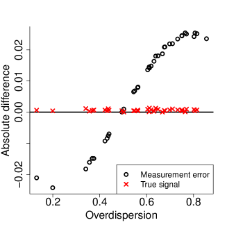
Figure 2: For vaccination coverages for the 37 admin1 areas in Nigeria, absolute differences in estimates for different cluster effect interpretations compared to the overdispersion assumption, plotted against estimates under the overdispersion assumption.

6.5 Admin1 estimates

We approximate the risk in area $a$ using the area $a$ specific version of Equation (6) with $\rho(\cdot)$ the population for children aged $[1,5)$ years, and $r_{\mathrm{S}}(\cdot)$ the smooth risk under the overdispersion interpretation. The smooth risk function is described in Section 5.3, and population density is defined on a $100\,\mathrm{m}\times 100\,\mathrm{m}$ with urban/rural assigned according to Section 5.4. Admin1 estimates of prevalence are produced according to the above procedure for the unit-level approaches, while direct estimation and the Fay-Herriot models directly produce estimates of the admin1 prevalences (since they are area-based methods).

A comparison between the direct estimates in Figure 3(a) and the covariate-based model UL-Cov in Figure 3(e) shows that the five covariates are not sufficient to capture the full spatial varation, and that random effects are necessary. With random effects included such as in UL-BYM(A1)-Cov, Figure 3(c) shows that estimates are visually indistinguishable from DE-Weighted. This is representative for the seven other unit-level models that include random effects and UL-Int has even less spatial variation than UL-Cov. The remaining estimates are shown in Appendix A.8.

Figure 3(b) shows that the direct estimates have high uncertainty as measured by the coefficient of variation (CV), Figure 3(d) shows that the spatial smoothing and covariates in UL-BYM(A1)-Cov reduces the uncertainty, whereas Figure 3(b) shows that using UL-Cov, which only includes covariates, results in artifically low uncertainty. The CV for the estimates from each approach are summarized in Figure 4(a). The direct estimates do not borrow strength across admin1 areas and have the highest uncertainty. The area-level models reduce the uncertainty somewhat by post-hoc smoothing of direct estimates across admin1 areas. The biggest reduction in variance happens in areas with high variance, and areas with low variance are not much affected by the post-hoc smoothing. For the four model-based approaches, estimation uncertainty is increasingly reduced as we model at finer and finer spatial scale. The changes in variation in CV values are mostly determined by area-level versus unit-level modelling, and when using unit-level models, the spatial resolution used for the spatial effect. Including covariates does not give major changes in the variation. The reduction in variance occurring when using unit-level models with spatial effects at finer spatial resolutions warrants further investigation because it may indicate oversmoothing of the sparse data.

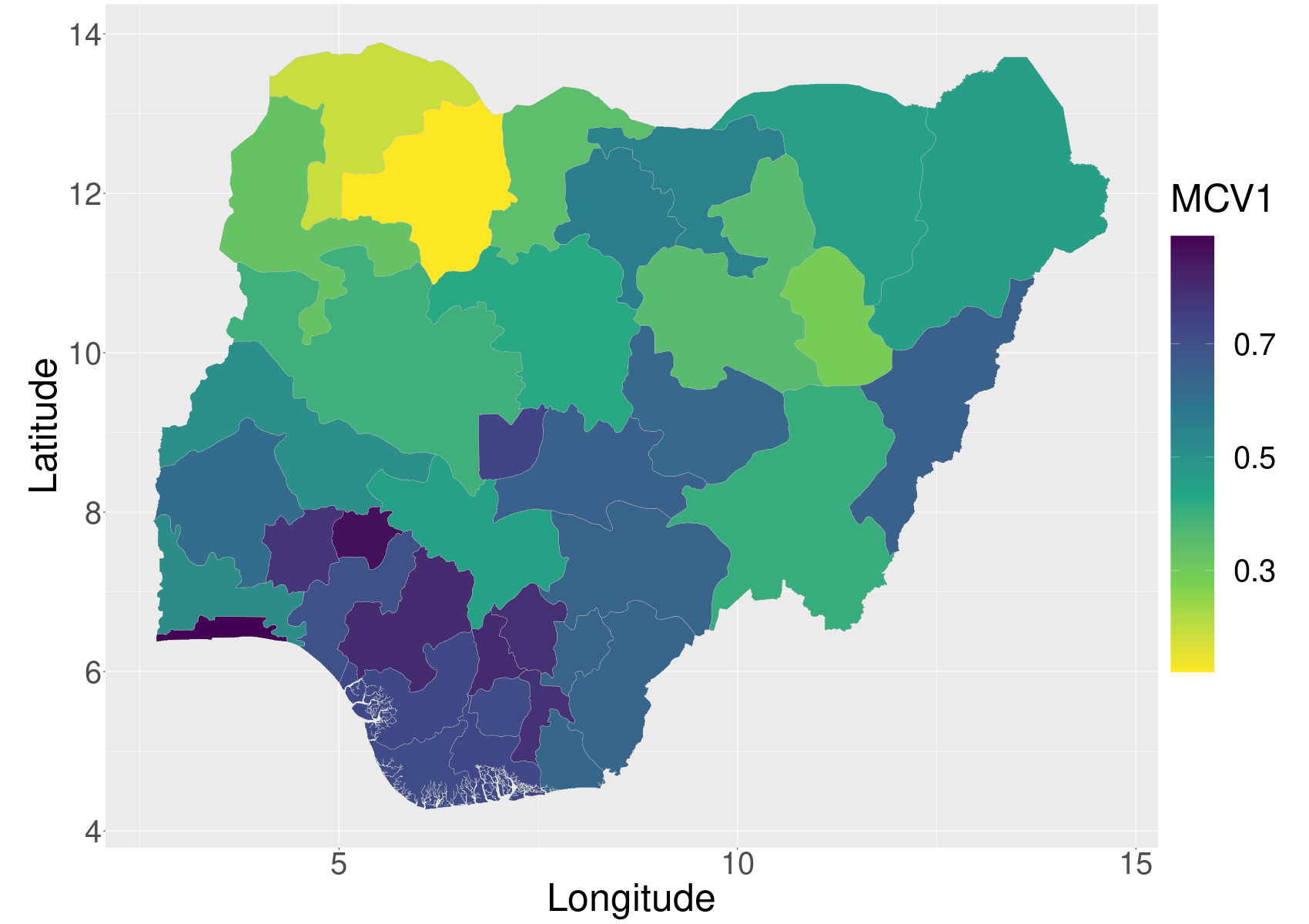
(a) MCV1 for DE-Weighted

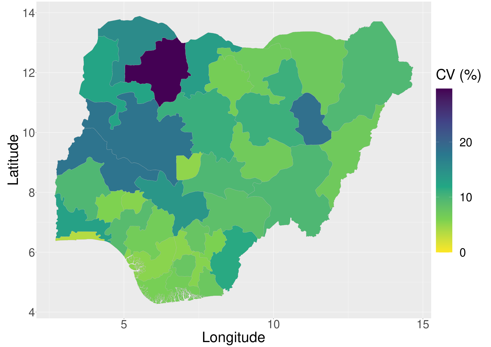
(b) CV for DE-Weighted

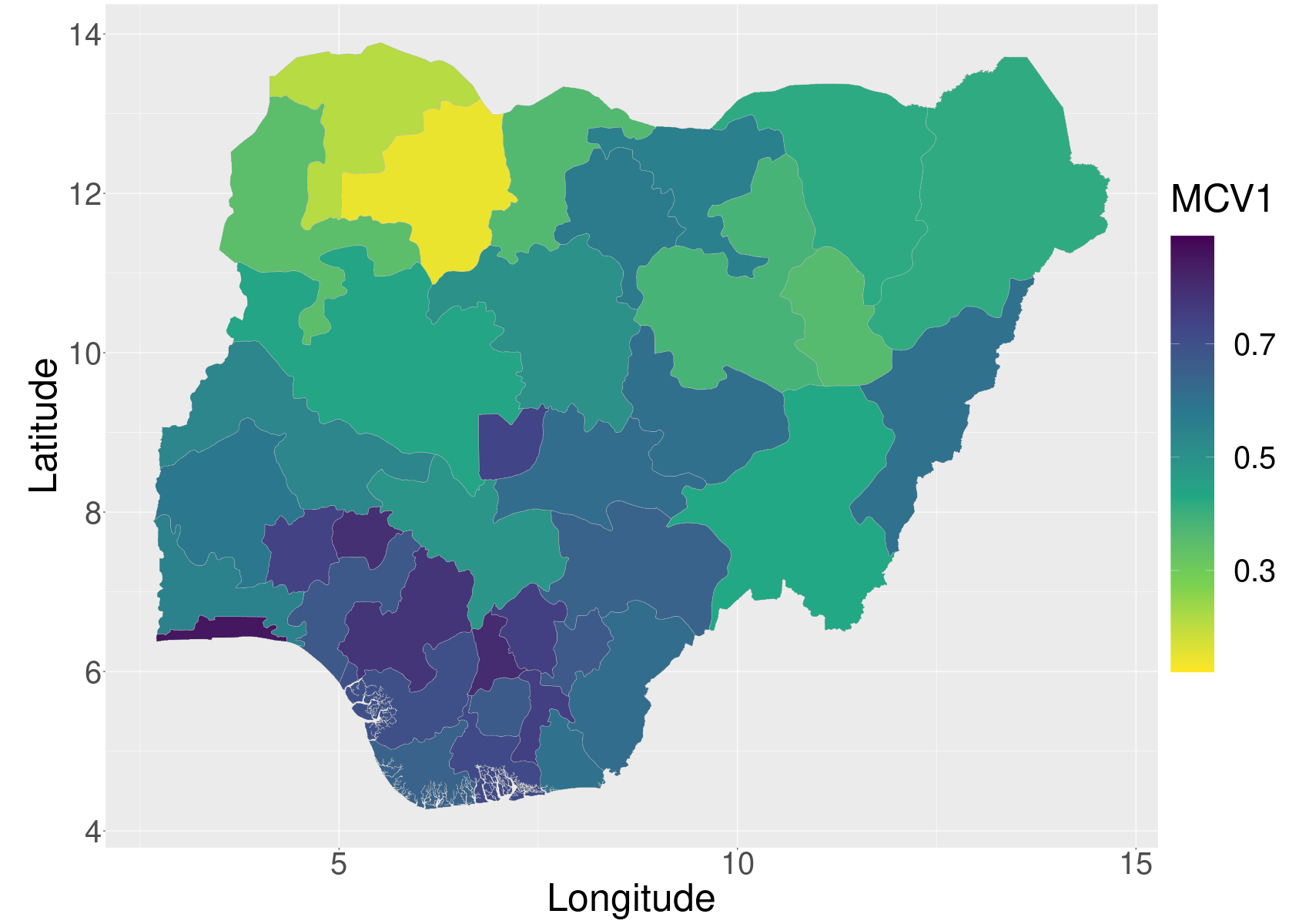
(c) MCV1 for UL-BYM(A1)-Cov

(d) CV for UL-BYM(A1)-Cov

(e) MCV1 for UL-Cov

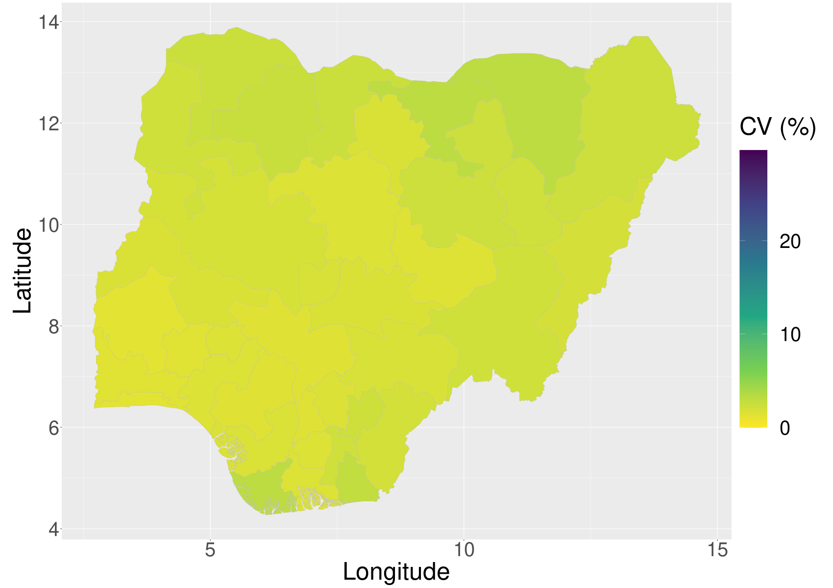
(f) CV for UL-Cov

Figure 3: Left: Estimates of MCV1. Right: coefficients of variation(CV) for vaccination coverage for the 37 admin1 areas using (row 1) DE-Weighted, (row 2) UL-BYM(A1)-Cov and (row 3) UL-Cov.

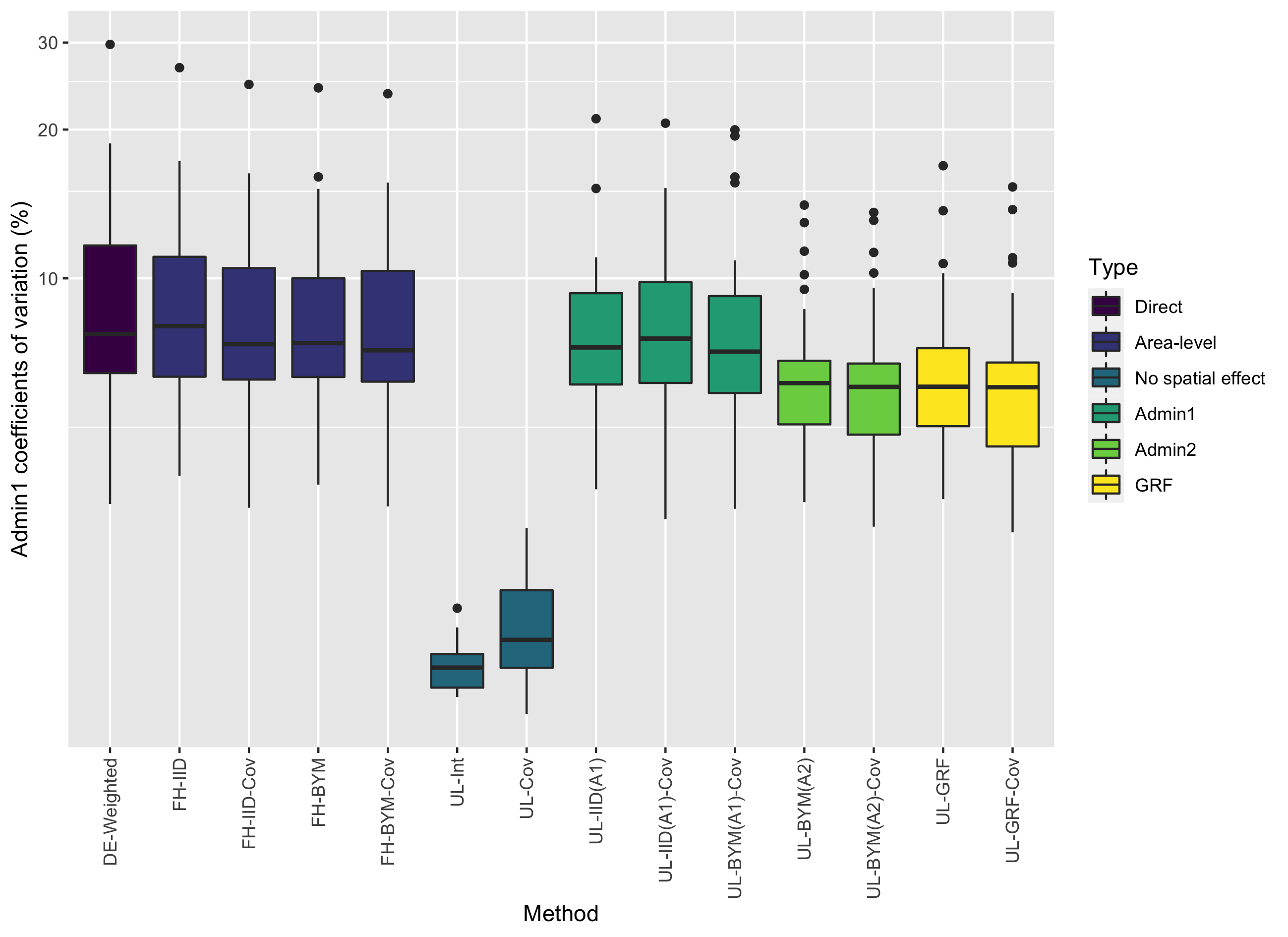
(a) Admin1 estimates

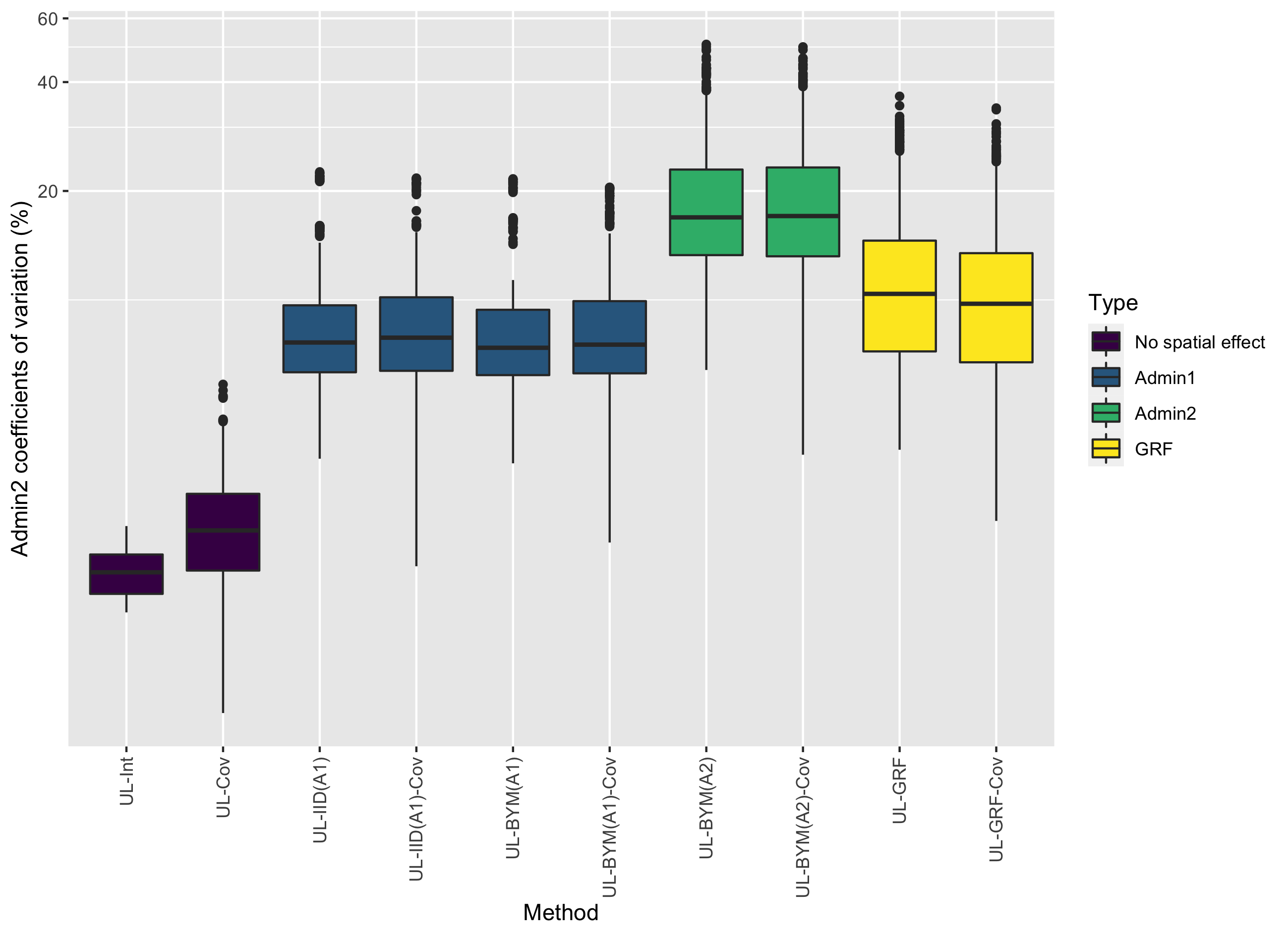
(b) Admin2 estimates

Figure 4: Boxplot of (a) the 37 coefficients of variation for each approach and (b) the 774 coefficients of variation for each approach.

6.6 Admin2 estimates

Figure 5 shows that UL-BYM(A1)-Cov allows some variation at admin2 through the covariates, but that the major changes occur when changing from admin1 areas to finer spatial scales for the random effects. Furthermore, the CV values are artificially low in some of the North-Eastern admin2 areas which have no observations. This is caused by sharing the spatial effect across all admin2 areas within the admin1 area. UL-BYM(A2)-Cov gives less sharp changes across admin1 boundaries since the spatial effect can take different values at each admin2 area. Furthermore, it correctly captures the fact that uncertainty should be higher at admin2 areas that have no observations. UL-GRF-Cov gives estimates that are much smoother than UL-BYM(A2)-Cov, and also reduces the CV values. This demonstrates that using a continuous space model implies much smoother behaviour than an admin2 model.

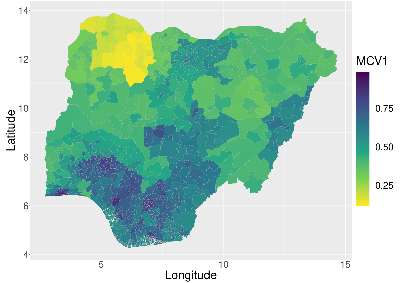
(a) MCV1 for UL-BYM(A1)-Cov.

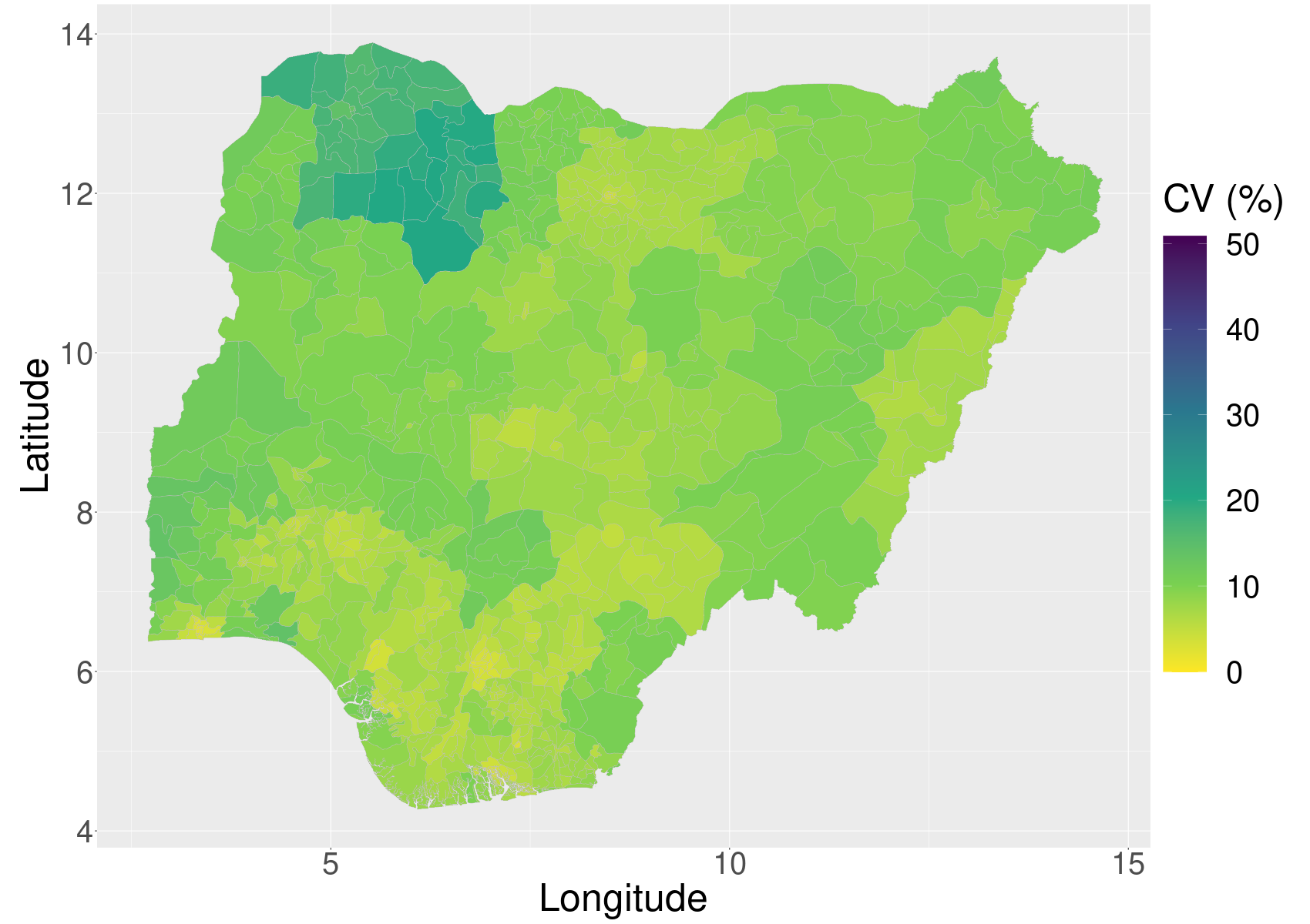
(b) CV for UL-BYM(A1)-Cov.

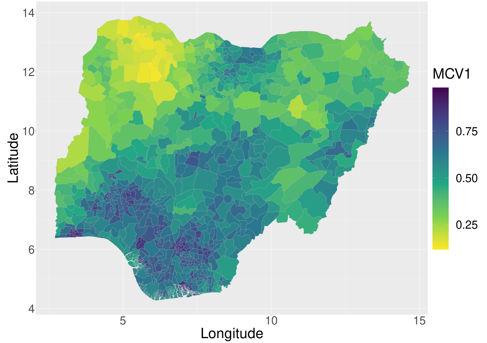
(c) MCV1 for UL-BYM(A2)-Cov.

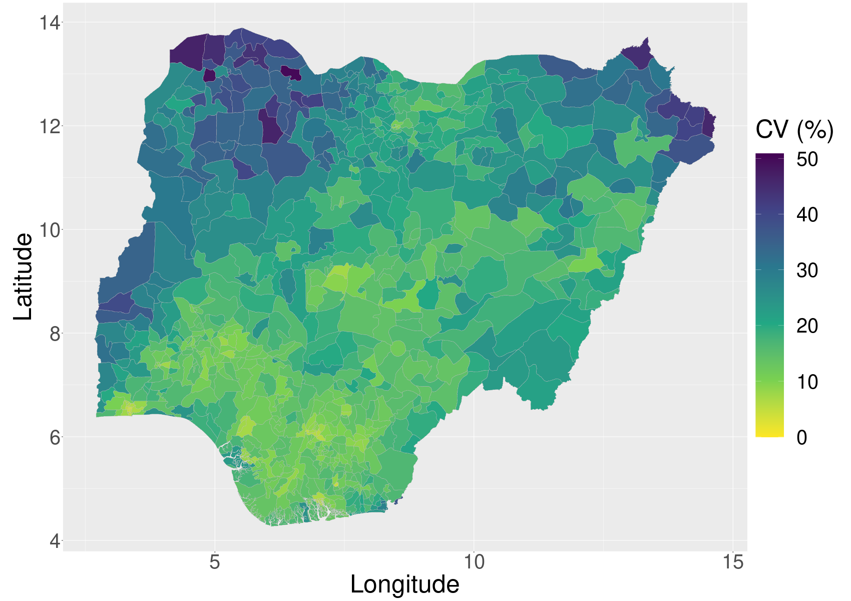
(d) CV for UL-BYM(A2)-Cov.

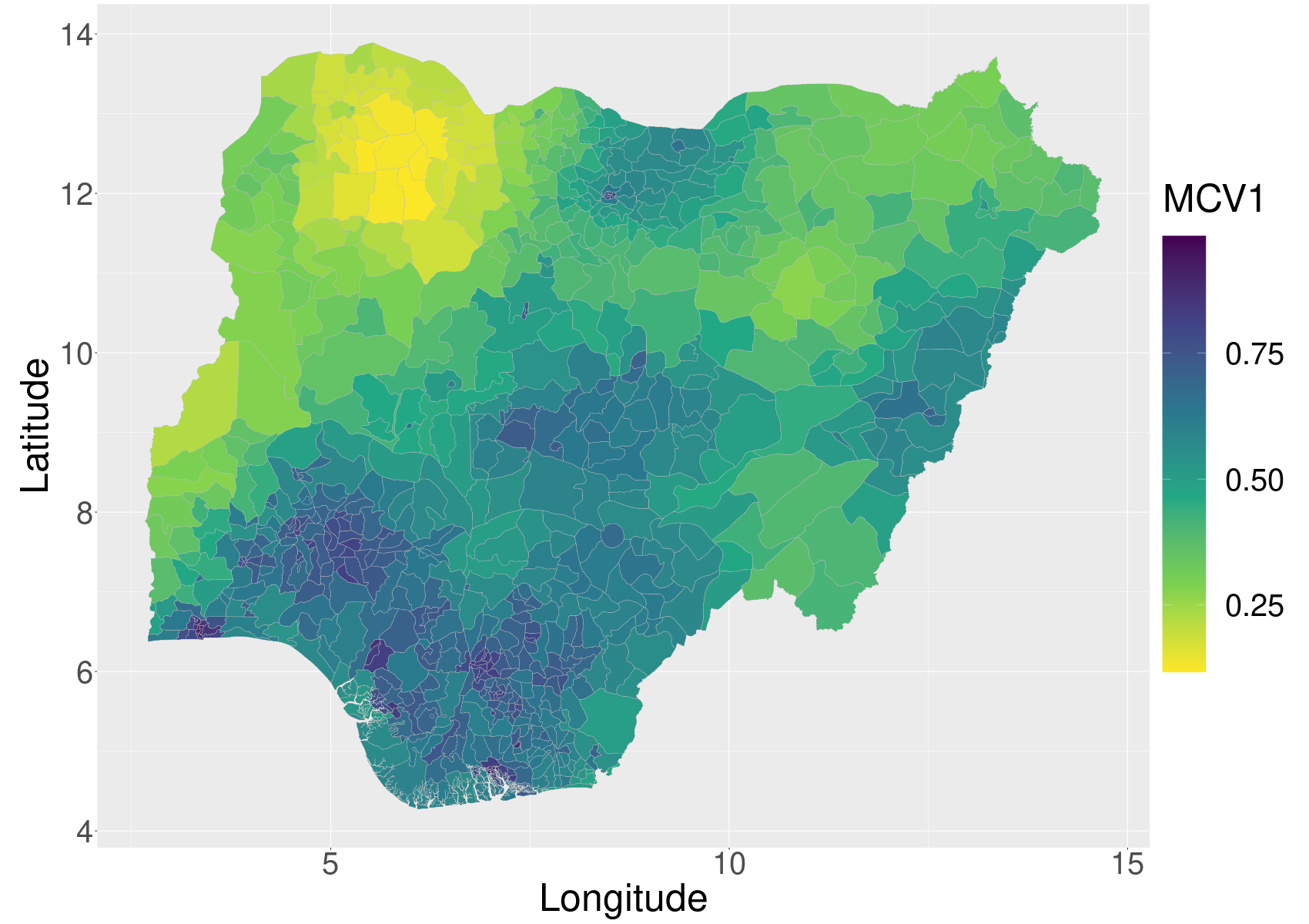
(e) MCV1 for UL-GRF-Cov.

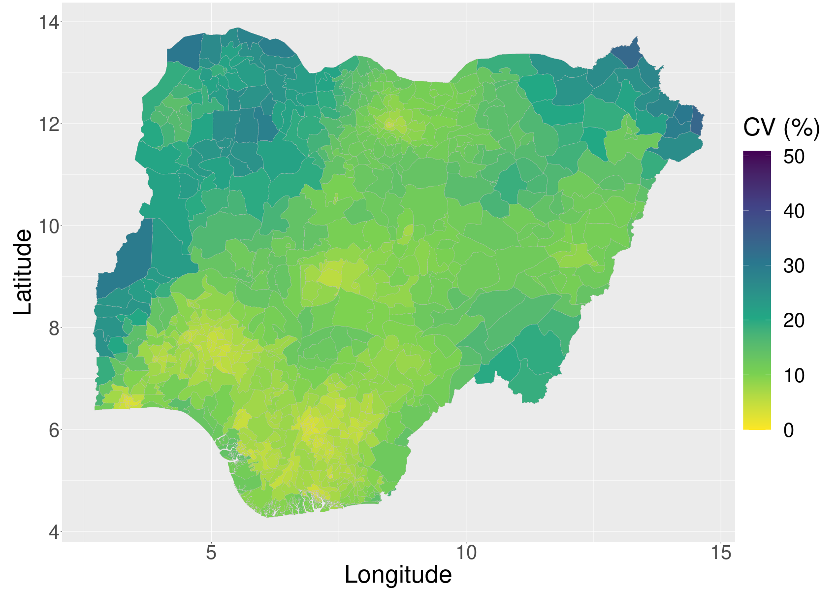
(f) CV for UL-GRF-Cov.

Figure 5: Left: Estimates of MCV1. Right: coefficients of variation(CV) for vaccination coverage for the 37 admin1 areas using (row 1) UL-BYM(A1)-Cov, (row 2) UL-BYM(A2)-Cov and (row 3) UL-GRF-Cov.

Including covariates gives only small differences in the estimates when the spatial effect varies at admin2 or in continuous space. However, the effect of including covariates is clear when the spatial effect exists at a coarser resolution than the target geography. See Appendix A.9 for figures of estimates and CV values for all models. Figure 4(b) shows that the key factor that influences the CV values are the resolution at which the spatial effects are included. Admin1 spatial effects, continuous space spatial effects, and admin2 spatial effects give increasing amounts of uncertainty.

6.7 Admin1 validation

The main target of our analysis is prevalences for administrative areas and we aim to assess the models’ ability to estimate these. We have sufficient power in the survey to make reliable direct estimates at admin1 areas and propose to view the direct estimates for admin1 areas as observations of the true vaccination coverages in the admin1 areas. From this perspective, the observation model for the logit of the direct estimate in area $a$, $Z_{a}=\text{logit}(\hat{P}_{a})$, is approximately Gaussian for large sample sizes. The expected value is approximately equal to the true logit of vaccination coverage, $\text{logit}(p_{a})$, and the estimated variance $\hat{V}_{a}$ is computed taking the complex survey design into account.

Each Bayesian model gives rise to a predictive distribution of the true logit vaccination coverage, $\pi(\text{logit}(p_{a})|\text{data})$. If we hold out clusters in area $a$ when fitting the model, the direct estimate is independent of the predictive distribution, and we can construct a predictive distribution of the direct estimate, $\pi(z_{a}|\text{data from other areas})$, which includes the uncertainty in the direct estimates. These can be used in a validation scheme where we compare the 37 hold-out predictive distributions of the direct estimates with the “observed” direct estimates being used to score the predictions.

We simplify scoring by assuming that the predictive distributions are Gaussian so that we only need to estimate the posterior mean and posterior standard deviation for each hold-out area. To assess the predictions we use the mean square error (MSE) and the log-score, both on the logit-scale. Given the normal observation model for the direct estimates, the difference between the MSE and log-score metrics is that the latter scale the sum of squares by the estimated variance of the direct estimates. See Appendix A.7 for further details. In addition, we compute the coverage for the hold-out areas as the proportion of the 37 direct estimates that are contained in the 95% credible intervals. Table 2 shows that for admin1-level validation, UL-BYM(A2)-Cov and UL-GRF-Cov are best in terms of MSE, but the coverages are 51% and 62%, respectively, which is well below the nominal level of 95%. This suggests that while mean square errors are better, the predictive distributions are less compatible with the observed direct estimates. UL-BYM(A1)-Cov is the best model in terms of MSE, log-score, and coverage. The results suggest that including covariates is helpful, but that modelling at fine resolution should not be done just because we have the ability to do so, but that one should keep the target of inference in mind when choosing the model, and that model validation is important. This point of view is supported by Corral et al., (2021) who suggest that random effects should be introduced at the level at which inference is desired.

The added value of admin1-level validation is clear when compared with standard 10-fold cross-validation. Here we randomly divide the 1324 clusters into 10 similarly sized sets, hold out one set at a time, fit the model to the remaining clusters, and predict the observed vaccination coverage for the hold-out clusters. MSE and log-scores are then computed cluster-wise and averaged across all clusters, and given in Table 3. This approach can barely distinguish between the approaches, and only detects that random effects are necessary and that there is a slight improvement when including covariates. This approach does not have the power to strongly differentiate between the spatial models due to the low number of trials in each cluster.

Table 2: Scores for hold-out predictions of direct estimates in the 37 admin1 areas. These were computed on logit-scale. Lower scores are better and coverage closer to nominal level is preferable.

Model	MSE	Log-score	Cvg. (95%)	Avg. CI len. (95%)
Fay-Herriot
FH-IID	0.814	1.34	92	3.35
FH-IID-Cov	0.397	1.00	92	2.43
FH-BYM	0.440	0.98	92	2.35
FH-BYM-Cov	0.355	0.92	95	2.25
Unit-level – covariates
UL-Int	0.619	4.37	3	0.15
UL-Cov	0.389	2.53	16	0.20
Unit-level – admin1
UL-IID(A1)	0.660	1.24	95	2.99
UL-IID(A1)-Cov	0.451	1.03	95	2.50
UL-BYM(A1)	0.378	0.91	97	2.28
UL-BYM(A1)-Cov	0.310	0.84	95	2.11
Unit-level – admin2
UL-BYM(A2)	0.342	1.08	57	1.08
UL-BYM(A2)-Cov	0.270	0.93	62	0.99
Unit-level – GRF
UL-GRF	0.361	1.18	62	1.07
UL-GRF-Cov	0.286	0.98	51	0.97

Table 3: Scores for 10-fold cluster-level cross-validation. Lower scores are better.

Model	MSE	Log-score
Unit-level – covariates
UL-Int	0.110	1.52
UL-Cov	0.099	1.46
Unit-level – admin1
UL-IID(A1)	0.089	1.40
UL-IID(A1)-Cov	0.087	1.39
UL-BYM(A1)	0.089	1.40
UL-BYM(A1)-Cov	0.087	1.38
Unit-level – admin2
UL-BYM(A2)	0.089	1.40
UL-BYM(A2)-Cov	0.088	1.39
Unit-level – GRF
UL-GRF	0.089	1.40
UL-GRF-Cov	0.087	1.39

7 Discussion

Subnational prevalence mapping entails the estimation of empirical proportions in administrative areas. Traditional SAE approaches directly target such proportions and estimation is intimately connected to the survey design under which the data was collected. However, successful application of these approaches hinges on sufficient power for direct estimation or sufficient power for indirect estimation through reliable auxiliary population information at the target resolution. This means that unit-level models cannot include spatial effects at finer resolutions than one has population sizes. For example, a cluster-level spatial effect requires knowledge about the locations and the population sizes of all EAs in order to predict the outcomes of the unobserved individuals in a consistent way. Thus, the SAE literature does not typically go beyond simple unstructured random effects or area-level random effects when modeling between-area variation.

Traditional geostatistical approaches take a different perspective. Models are expressed in terms of risk with the aim being to describe the outcome at any spatial location. Since the data source is point-referenced, this motivates the use of spatial models in continuous space. Such models have the potential to provide detailed maps of the spatial variation in risk, but areal estimates cannot be produced without detailed auxiliary population information and one has to consider the sampling design.

There is a strong and growing desire to produce official subnational estimates of demographic and health indicators. When producing official statistics using SAE, Tzavidis et al., (2018) suggest that one consider progressively finer geographies while at each level assessing the feasibility of producing SAE estimates for the current level. In our experience, for estimation when the data are rich, for example when constructing national estimates using DHS or MICS surveys, direct (weighted) estimation is a reliable approach. This offers asymptotic (design) consistency and the inclusion probabilities encompass all the necessary information to estimate a national prevalence. As mentioned, the weighted estimates implicitly encode the relevant population information (the weights were constructed from the sampling frame), and target empirical proportions. In the context of LMICs, reliable covariate information is limited, and at admin1 one should first consider areal Fay-Herriot SAE models such as Mercer et al., (2015), and if the survey does not provide reliable admin1 estimates using SAE, one should apply spatial smoothing. For finer levels such as admin2 or pixel maps, one should generally use spatial statistical methods, but ensure that the model contains terms to acknowledge the complex design. The key point here is that the goal of the analysis should determine the approach, and different goals may call for different approaches.

Complex survey designs lead to spatially varying sampling efforts. This resembles geostatistical preferential sampling (Diggle et al.,, 2010), but in survey sampling, the inclusion probabilities are not directly linked to the level of risk in the clusters. The inclusion probabilities are instead determined by a survey design that aims to reach the desired statistical power for areas of interest in a cost efficient way. This does not mean that the survey design should be haphazardly ignored, however. Most household surveys are stratified on the basis of urban/rural, and it is commonplace for the outcome to be associated with this classification. We have chosen to acknowledge the stratification in spatial models using covariates and area effects.

Aggregation is a major challenge even without the presence of a complex survey design. For example, if one disaggregates areas into rural and urban, it is necessary to construct reliable aggregation weights for combining the rural and urban estimates in each area. Estimating an urban/rural association is relatively uncomplicated, but producing reliable fine-scale maps of urban/rural, which are needed for spatial aggregation, is an ongoing research problem. Treating space as continuous, increases the challenge as one needs to rely on fine-scale population density rasters to perform aggregation to the areal level. Both population and covariate rasters are estimated based on other data sources, and there is a need for further investigation to understand the consequences of not acknowledging the inherent uncertainty when used in an aggregation scheme. The result of aggregation is typically an areal risk and an examination of the importance of distinguishing between risk and prevalence at different spatial scales would be worthwhile. These open issues motivate our suggestion for spatial modelling at the target administrative level unless the stratification necessitates modelling at finer scales. Corral et al., (2021) reached a similar conclusion.

Section 6 demonstrates the clear importance of model choices both in terms of central predictions and uncertainty. Since it will always be possible to argue for many reasonable models, we need formal validation techniques to compare different models in terms of their ability to estimate areal prevalences. However, the spatial misalignment between the point-referenced observations and the desired areal quantities makes validation a challenging task. We propose a model validation approach that frames direct estimates as observations and scores different models based on their ability to predict direct estimates. One should be wary of using more complex models unless one can show they are better than simpler models through validation. In the case study, we observe that modelling at finer spatial scales than the target administrative level, gave rise to poorer prediction scores. In particular, a continuously-indexed risk surface performed more poorly than a model with constant risk in each administrative area. As an extreme example, if we wanted a national estimate, we would not use spatial models and aggregate, but simply calculate a weighted estimate. There are cases in which a continuously-indexed model is necessary for a principled way to handle data that is available with limited geographical information (e.g., area only information and not points) or under different geographical partitions (Marquez and Wakefield,, 2021; Wilson and Wakefield,, 2020).

There are several other important aspects that have not been addressed in this paper, and require further research. In particular, spatio-temporal analysis may require the combination of surveys from different sampling frames. This further complicates the issue of urban/rural stratification because the definitions of urban/rural in the sampling frames will most likely give rise to different geographic stratfications. One may then stratify the model by urban/rural crossed by sampling frame, but the question is how to combine estimates for different sampling frames into a single estimate? Additionally, a common technique in survey statistics is poststratification whereby inclusion probabilities are adjusted to account for known structures in the population such as the proportion of males to females. It is not obvious how to adjust the aggregation schemes in a similar way for geostatistical models, but poststratification is less common in LMICs since such information is not sufficiently reliable. The fact that the GPS coordinates provided to the public have been jittered is another source for concern, but the amount is always small compared to the size of a country. Finally, benchmarking the subnational estimates to officially accepted national levels may be necessary (Särndal,, 2007; Zhang and Bryant,, 2020), and non-sampling errors such as recollection bias and migration of interview subjects may bias estimates.

A more complex space-time discrete hazards model has been used to produce spatio-temporal estimates of the under-5 mortality rate (U5MR) for 22 LMICs (UN IGME,, 2021). A key focus for these estimates was to consider each country separately, rather than a joint model for multiple countries (as practiced by IHME, see for example, Burstein et al., (2018)). This is important as some countries require specific considerations such as adjustments due to natural disasters or conflicts. There is still work to be done in making such estimates a tool that routinely guides policy decisions. We believe a key focus should be on transparent methods and software such as SUMMER (Li et al.,, 2021) that can be reproducibly run by national statistics’ offices. Software should be accompanied with development of detailed vignettes. This is consistent with the GATHER statement (Stevens et al.,, 2016). We have recently partnered with researchers at DHS to produce guidelines and code scripts to routinely produce subnational child mortality estimates (Wu et al.,, 2021).

We believe that the way forward for prevalence mapping is to bridge the rich literatures of SAE and spatial statistics. The aim should be a synthesis which exploits the broad range of techniques from spatial statistics to overcome data sparsity, but at the same time acknowledges the design and the subnational areal targets of inference, which are often empirical averages. As a step in this direction, we have presented an approach that is framed from a spatial statistics perspective, but includes cluster effects to acknowledge clustering, and urban/rural fixed effects and a piece-wise constant risk surface to acknowledge stratification. The latter is similar to the inclusion of fixed effects to acknowledge stratification, but induces spatial smoothing. The approach is not fully design-consistent, and does not capture all aspects of the inclusion probabilities or make non-response adjustments. However, we believe it is an important step towards spatial modelling with a clear understanding of the importance of the survey design, which has too often been downplayed.

Appendix A Supplementary Details for Spatial Estimation of Vaccination Coverage in Nigeria

This section provides supplementary details on the sampling frame and covariates, full model details, and more details on the scores used for validation. The admin1 and admin 2 estimates from all models are shown in Section A.8 and Section A.9, respectively.

A.1 Details on enumeration areas

The 2006 census in Nigeria divided Nigeria into 664999 EAs. Table A.1 shows how these EAs disaggregate into the 37 admin1 areas crossed by urban/rural. Note that the classifications of these EAs were updated before the Nigeria 2018 DHS (NDHS2018) survey was conducted (National Population Commission - NPC and ICF,, 2019, Appendix A.2).

Table A.1: Number of EAs classified as urban and rural for each admin1 area in the 2006 census. In total, 276058 urban EAs and 388941 rural EAs.

Admin1	Urban	Rural
Abia	2106	9463
Adamawa	2820	9988
Akwa Ibom	908	16205
Anambra	18409	3498
Bauchi	2761	17124
Bayelsa	2628	6379
Benue	2006	20850
Borno	7798	16288
Cross River	1410	14912
Delta	9008	9201
Ebonyi	11911	1977
Edo	7964	4829
Ekiti	9438	2123
Enugu	9774	4223
FCT Abuja	2452	1138
Gombe	1955	7539
Imo	10006	9567
Jigawa	2293	18900
Kaduna	9529	12263

Admin1	Urban	Rural
Kano	16957	19402
Katsina	6874	26442
Kebbi	14020	2621
Kogi	5492	10354
Kwara	11715	4556
Lagos	25424	0
Nasarawa	2008	7211
Niger	5126	18319
Ogun	7085	7408
Ondo	8588	10667
Osun	19810	6097
Oyo	22405	8701
Plateau	3949	11930
Rivers	12480	12381
Sokoto	2548	10231
Taraba	1657	8943
Yobe	3053	11870
Zamfara	3090	13942

A.2 Covariate rasters

We use two covariate rasters:

• Poverty: Worldpop 2010 estimates of proportion of people per grid square living in poverty, as defined by $2 a day threshold. URL: https://www.worldpop.org/geodata/summary?id=1267.

• Access: Malaria Mapping Project 2015 Map of Travel Time to Cities. URL: https://malariaatlas.org/explorer/. (Weiss et al.,, 2018).

Both covariates are converted to matching $1\,\mathrm{km}\times 1\,\mathrm{km}$ rasters that covers Nigeria. The values are shown in Figure A.1. The major pattern in the poverty covariate is that it is relatively stable over rural areas, but that some urban areas such as the capital has much lower poverty.

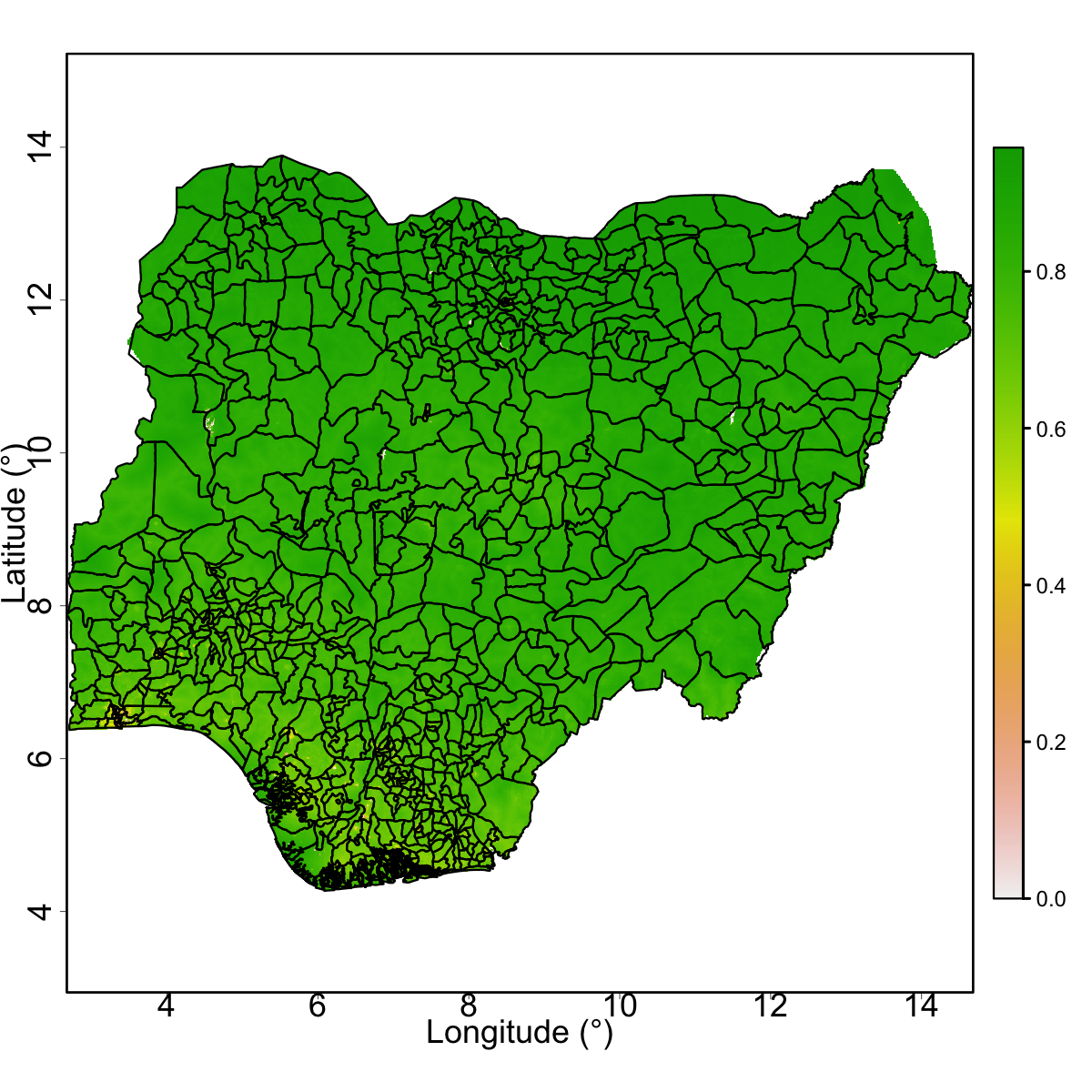
(a) Poverty

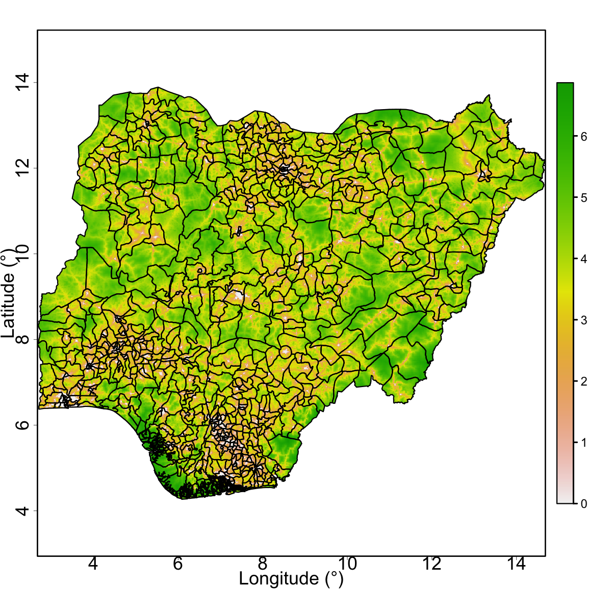
(b) log1p(Travel-time)

Figure A.1: The two covariate rasters: proportion of people per $1\,\text{km}\times 1\,\text{km}$ grid cell living in poverty (as defined by $2 per day), and the $\text{log1p}(x)=\text{log}(1+x)$ transformation of travel-time to nearest city.

A.3 Urban/rural classification

Using the procedure described in the main paper, we constructed a $100\,\mathrm{m}\times 100\,\mathrm{m}$ raster with values 1 (urban) and 0 (rural). The raster is a refinement of the covariate rasters in Section A.2 such that each $1\,\text{km}\times 1\,\text{km}$ grid cell is divided into 100 smaller grid cells. The resulting raster is shown in Figure A.2.

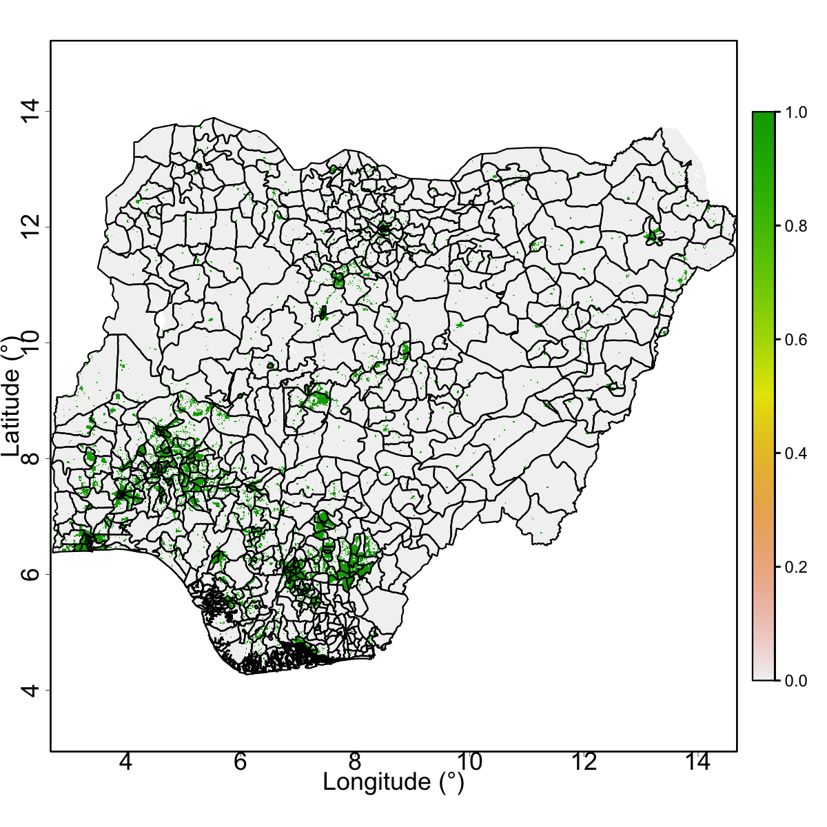
Figure A.2: $100\,\text{m}\times 100\,\text{m}$ raster of estimated urban and rural grid cells for NDHS2018 sampling frame. Green is urban and grey is rural.

A.4 Full model details

In this section, we denote cluster index by $c=1,\ldots,m$, where $m=1324$ is the number of clusters, and we denote the location of cluster $c$ by $\boldsymbol{s}_{c}$. The number of areas in the administrative level is $A$ and the individual areas are indexed by $a=1,\ldots,A$. Throughout the section, we assume that the cluster index run over all possible values unless otherwised specified. Observations consist of number of children $n_{c}$ and number of children vaccinated $y^{\mathrm{cl}}_{c}$. Let $p_{a}$ denote the prevalence in area $a$ for $a=1,\ldots,A$.

A.4.1 Direct estimation

Direct estimates that account for the complex survey design are computed using the R-package survey (Lumley,, 2018). This provides estimates $\widehat{\text{logit}(p_{a})}$ with associated variance estimates $\hat{V}_{a}$. We assume that the sample distributions (under repeated sampling under the survey design) are given by $\widehat{\text{logit}(P_{a})}\sim\mathcal{N}(\text{logit}(p_{a}),\hat{V}_{a})$. The estimates are independent between regions as the estimates are based on independent data. This model is denoted DE-Weighted in the main paper.

A.4.2 Area-level models

Let $\hat{P}_{a}^{\mathrm{HT}}$, $a=1,\ldots,37$, be the Hájek estimators used to produce the direct estimates for each admin1 area in Section A.4.1, and let $Z_{a}=\log(\hat{P}_{a}^{\mathrm{HT}})$. The four Fay-Herriot (FH) type models use

$$Z_{a}=\alpha+\boldsymbol{x}_{a}^{\mathrm{T}}\boldsymbol{\beta}+\delta_{a}+\epsilon_{a},\quad a=1,\ldots,37,$$ (10)

where $\alpha\sim\mathcal{N}(0,1000)$ is the intercept, $\boldsymbol{x}_{a}$ is a $k$-dimensional vector of areal covariates associated with each admin1 area, $\boldsymbol{\beta}\sim\mathcal{N}_{k}(\boldsymbol{0},1000\mathbf{I}_{k})$, and $\epsilon_{a}\sim\mathcal{N}(0,\hat{V}_{a})$, independently for $a=1,\ldots,37$, where $\hat{V}_{a}$ is the design-based estimate of the variance of $Z_{a}$. $\boldsymbol{\delta}=(\delta_{1},\ldots,\delta_{37})^{\mathrm{T}}$ is a Gaussian random effect whose interpretation varies in the four models. Here we assume that $\mathrm{logit}(p_{a})=\alpha+\boldsymbol{x}_{a}^{\mathrm{T}}\boldsymbol{\beta}+\delta_{a}$ and that $\epsilon_{a}$ is the sampling error.

Let BYM2 (Riebler et al.,, 2016) refer to the model

$$\boldsymbol{\delta}=\sigma_{\delta}(\phi_{\mathrm{s}}\boldsymbol{v}+\sqrt{1-\phi_{\mathrm{s}}^{2}}\boldsymbol{u}),$$

where $\boldsymbol{v}\sim\mathcal{N}_{37}(\boldsymbol{0},\mathbf{I}_{37})$, and $\boldsymbol{u}$ is a rescaled Besag model on the admin1 areas that has representative variance around 1 (Sørbye and Rue,, 2014). We create four types of FH models by varying the number of covariates included and the model for $\boldsymbol{\delta}$:

• FH-IID: no covariates ($\boldsymbol{x}_{a}$ is not included in Equation (10)), and $\boldsymbol{\delta}\sim\mathcal{N}_{37}(0,\sigma_{\delta}^{2}\mathbf{I}_{37})$;

• FH-IID-Cov: five areal covariates in $\boldsymbol{x}_{a}$, and $\boldsymbol{\delta}\sim\mathcal{N}_{37}(0,\sigma_{\delta}^{2}\mathbf{I}_{37})$;

• FH-BYM: no covariates ($\boldsymbol{x}_{a}$ is not included in Equation (10)), and $\boldsymbol{\delta}$ is the BYM2 model;

• FH-BYM-Cov: five areal covariates in $\boldsymbol{x}_{a}$, and $\boldsymbol{\delta}$ is the BYM2 model.

For FH-IID and FH-IID-Cov, we use a PC prior (Simpson et al.,, 2017) with hyperparameter set so that $\mathrm{P}(\sigma_{\delta}>1)=0.05$, and for FH-BYM and FH-BYM-Cov, we use a PC prior (Riebler et al.,, 2016) with hyperparameters set by $\mathrm{P}(\phi_{\mathrm{s}}>0.5)=0.5$ and $\mathrm{P}(\sigma_{\delta}>1)=0.05$.

A.4.3 Unit-level models

The unit level models vary depending on i) covariates or not covariates, ii) the spatial resolution used for modelling, and iii) whether structured or unstructured random effects are used. From a geostatistical/spatial statistics perspective all unit-level models that we consider share the form

$$Y_{c}^{\mathrm{cl}}|r_{c},n_{c} \sim\text{Binomial}(n_{c},r_{c}),$$

$$\text{logit}(r_{c}) =\eta(\boldsymbol{s})+\epsilon_{c},\quad c=1,\ldots,m,$$

$$\boldsymbol{\eta}(\boldsymbol{s}) =\alpha+\boldsymbol{x}(\boldsymbol{s})^{\mathrm{T}}\boldsymbol{\beta}+u(\boldsymbol{s}),\quad\boldsymbol{s}\in\mathcal{D}\subset\mathbb{R}^{2},$$

where $\epsilon_{1},\ldots,\epsilon_{m}\overset{\text{iid}}{\sim}\mathcal{N}(0,\sigma_{\mathrm{N}}^{2})$, $\alpha\sim\mathcal{N}(0,1000)$, $\boldsymbol{x}_{a}$ is a covariate vector of length $k$, $\boldsymbol{\beta}\sim\mathcal{N}_{k}(0,1000\mathbf{I}_{k})$, $u(\cdot)$ is a Gaussian random field (GRF) that will be described for each model, and $\mathcal{D}$ is the geographic area describing Nigeria. We use the a PC prior for $\sigma_{\mathrm{N}}^{2}$ (Simpson et al.,, 2017) with hyperparameter specified by $\mathrm{P}(\sigma_{\mathrm{N}}>1)=0.05$.

The two models without any random effects are

• UL-Int: The spatially varying linear predictor is

  $$\boldsymbol{\eta}(\boldsymbol{s})=\alpha+\boldsymbol{x}(\boldsymbol{s})^{\mathrm{T}}\boldsymbol{\beta},\quad\boldsymbol{s}\in\mathcal{D},$$

  where $\boldsymbol{x}(\boldsymbol{s})$ has one covariate giving rural (0) or urban (1), and $u(\cdot)$ is excluded.

• UL-Int-Cov: The spatially varying linear predictor is

  $$\boldsymbol{\eta}(\boldsymbol{s})=\alpha+\boldsymbol{x}(\boldsymbol{s})^{\mathrm{T}}\boldsymbol{\beta},\quad\boldsymbol{s}\in\mathcal{D},$$

  where $\boldsymbol{x}(\boldsymbol{s})$ has five covariates, and $u(\cdot)$ is excluded.

The four models at admin1 resolution additionally contains parameters describing the marginal variance, $\sigma_{\mathrm{s}}^{2}>0$, and the proportion of $\sigma_{\mathrm{s}}^{2}$ that is structured, $0\leq\phi_{\mathrm{s}}\leq 1$. The models are:

• UL-IID(A1) The spatially varying linear predictor is

  $$\boldsymbol{\eta}(\boldsymbol{s})=\alpha+\boldsymbol{x}(\boldsymbol{s})^{\mathrm{T}}\boldsymbol{\beta}+\sigma_{\mathrm{s}}\delta_{a[\boldsymbol{s}]},\quad\boldsymbol{s}\in\mathcal{D},$$

  where $\boldsymbol{x}(\boldsymbol{s})$ has one covariate giving rural (0) or urban (1), $a[\boldsymbol{s}]$ denotes the admin1 area that location $\boldsymbol{s}$ belongs to, and $\delta_{1},\ldots,\delta_{37}\overset{\text{iid}}{\sim}\mathcal{N}(0,1)$.

• UL-IID(A1)-Cov The spatially varying linear predictor is

  $$\boldsymbol{\eta}(\boldsymbol{s})=\alpha+\boldsymbol{x}(\boldsymbol{s})^{\mathrm{T}}\boldsymbol{\beta}+\sigma_{\mathrm{s}}\delta_{a[\boldsymbol{s}]},\quad\boldsymbol{s}\in\mathcal{D},$$

  where $\boldsymbol{x}(\boldsymbol{s})$ has five covariates, $a[\boldsymbol{s}]$ denotes the admin1 area that location $\boldsymbol{s}$ belongs to, and $\delta_{1},\ldots,\delta_{37}\overset{\text{iid}}{\sim}\mathcal{N}(0,1)$.

• UL-BYM(A1) The spatially varying linear predictor is

  $$\boldsymbol{\eta}(\boldsymbol{s})=\alpha+\boldsymbol{x}(\boldsymbol{s})^{\mathrm{T}}\boldsymbol{\beta}+\sigma_{\mathrm{s}}(\phi_{\mathrm{s}}v_{a}+\sqrt{1-\phi_{\mathrm{s}}^{2}}\delta_{a[\boldsymbol{s}]}),\quad\boldsymbol{s}\in\mathcal{D},$$

  where $\boldsymbol{x}(\boldsymbol{s})$ has one covariate giving rural (0) or urban (1), $a[\boldsymbol{s}]$ denotes the admin1 area that location $\boldsymbol{s}$ belongs to, $\delta_{1},\ldots,\delta_{37}\overset{\text{iid}}{\sim}\mathcal{N}(0,1)$, and $\boldsymbol{v}=(v_{1},\ldots,v_{37})$ is a Besag model on admin1 areas scaled such that the representative variance is 1 (Sørbye and Rue,, 2014).

• UL-BYM(A1)-Cov The spatially varying linear predictor is

  $$\boldsymbol{\eta}(\boldsymbol{s})=\alpha+\boldsymbol{x}(\boldsymbol{s})^{\mathrm{T}}\boldsymbol{\beta}+\sigma_{\mathrm{s}}(\phi_{\mathrm{s}}v_{a}+\sqrt{1-\phi_{\mathrm{s}}^{2}}\delta_{a[\boldsymbol{s}]}),\quad\boldsymbol{s}\in\mathcal{D},$$

  where $\boldsymbol{x}(\boldsymbol{s})$ has five covariates, $a[\boldsymbol{s}]$ denotes the admin1 area that location $\boldsymbol{s}$ belongs to, $\delta_{1},\ldots,\delta_{37}\overset{\text{iid}}{\sim}\mathcal{N}(0,1)$, and $\boldsymbol{v}=(v_{1},\ldots,v_{37})$ is a Besag model on admin1 areas scaled such that the representative variance is 1 (Sørbye and Rue,, 2014).

For UL-IID(A1) and FH-IID(A1)-Cov, we use a PC prior (Simpson et al.,, 2017) with hyperparameter set so that $\mathrm{P}(\sigma_{\mathrm{s}}>1)=0.05$, and for UL-BYM(A1) and UL-BYM(A1)-Cov, we use a PC prior (Riebler et al.,, 2016) with hyperparameters set by $\mathrm{P}(\phi_{\mathrm{s}}>0.5)=0.5$ and $\mathrm{P}(\sigma_{\mathrm{s}}>1)=0.05$.

The two models at admin2 resolution additionally contains parameters describing the marginal variance, $\sigma_{\mathrm{s}}^{2}>0$, and the proportion of $\sigma_{\mathrm{s}}^{2}$ that is structured, $0\leq\phi_{\mathrm{s}}\leq 1$. The models are:

• UL-BYM(A2) The spatially varying linear predictor is

  $$\boldsymbol{\eta}(\boldsymbol{s})=\alpha+\boldsymbol{x}(\boldsymbol{s})^{\mathrm{T}}\boldsymbol{\beta}+\sigma_{\mathrm{s}}(\phi_{\mathrm{s}}v_{a}+\sqrt{1-\phi_{\mathrm{s}}^{2}}\delta_{a[\boldsymbol{s}]}),\quad\boldsymbol{s}\in\mathcal{D},$$

  where $\boldsymbol{x}(\boldsymbol{s})$ has one covariate giving rural (0) or urban (1), $a[\boldsymbol{s}]$ denotes the admin2 area that location $\boldsymbol{s}$ belongs to, $\delta_{1},\ldots,\delta_{774}\overset{\text{iid}}{\sim}\mathcal{N}(0,1)$, and $\boldsymbol{v}=(v_{1},\ldots,v_{774})$ is a Besag model on admin2 areas scaled such that the representative variance is 1 (Sørbye and Rue,, 2014).

• UL-BYM(A2)-Cov The spatially varying linear predictor is

  $$\boldsymbol{\eta}(\boldsymbol{s})=\alpha+\boldsymbol{x}(\boldsymbol{s})^{\mathrm{T}}\boldsymbol{\beta}+\sigma_{\mathrm{s}}(\phi_{\mathrm{s}}v_{a}+\sqrt{1-\phi_{\mathrm{s}}^{2}}\delta_{a[\boldsymbol{s}]}),\quad\boldsymbol{s}\in\mathcal{D},$$

  where $\boldsymbol{x}(\boldsymbol{s})$ has five covariates, $a[\boldsymbol{s}]$ denotes the admin2 area that location $\boldsymbol{s}$ belongs to, $\delta_{1},\ldots,\delta_{774}\overset{\text{iid}}{\sim}\mathcal{N}(0,1)$, and $\boldsymbol{v}=(v_{1},\ldots,v_{774})$ is a Besag model on admin2 areas scaled such that the representative variance is 1 (Sørbye and Rue,, 2014).

For UL-IID(A2) and FH-IID(A2)-Cov, we use a PC prior (Simpson et al.,, 2017) with hyperparameter set so that $\mathrm{P}(\sigma_{\mathrm{s}}>1)=0.05$, and for UL-BYM(A2) and UL-BYM(A2)-Cov, we use a PC prior (Riebler et al.,, 2016) with hyperparameters set by $\mathrm{P}(\phi_{\mathrm{s}}>0.5)=0.5$ and $\mathrm{P}(\sigma_{\mathrm{s}}>1)=0.05$.

The two models in continuous space (or pixel level resolution) includes a GRF that has an covariance function that is approximately Matérn with smoothness equals 1, marginal variance $\sigma_{\mathrm{s}}^{2}>0$, and spatial range $\rho_{s}>0$. The GRF is implemented through the SPDE approach (Lindgren et al.,, 2011) and uses the mesh discussed in Section A.5. The models are:

• UL-GRF: The spatially varying linear predictor is

  $$\boldsymbol{\eta}(\boldsymbol{s})=\alpha+\boldsymbol{x}(\boldsymbol{s})^{\mathrm{T}}\boldsymbol{\beta}+u(\boldsymbol{s}),\quad\boldsymbol{s}\in\mathcal{D},$$

  where $\boldsymbol{x}(\boldsymbol{s})$ has one covariate giving rural (0) or urban (1), and $u(\cdot)$ is a Matérn GRF with smoothness equals 1, marginal variance $\sigma_{\mathrm{s}}^{2}>0$, and spatial range $\rho_{s}>0$.

• UL-GRF-Cov: The spatially varying linear predictor is

  $$\boldsymbol{\eta}(\boldsymbol{s})=\alpha+\boldsymbol{x}(\boldsymbol{s})^{\mathrm{T}}\boldsymbol{\beta}+u(\boldsymbol{s}),\quad\boldsymbol{s}\in\mathcal{D},$$

  where $\boldsymbol{x}(\boldsymbol{s})$ has five covariates, and $u(\cdot)$ is a Matérn GRF with smoothness equals 1, marginal variance $\sigma_{\mathrm{s}}^{2}>0$, and spatial range $\rho_{s}>0$.

For UL-GRF and UL-GRF-Cov, we use the PC prior for Matérn GRFs (Fuglstad et al.,, 2019), where hyperparameters are specified by $\mathrm{P}(\sigma_{\mathrm{s}}>0.5)=0.5$ and $\mathrm{P}(\rho_{\mathrm{s}}>3)=0.5$.

A.5 Triangulation used for SPDE approach

We implement an approximate Matérn GRF using the SPDE approach (Lindgren et al.,, 2011). This is a common way to achieve computational efficiency in the geostatistical approaches (Utazi et al.,, 2020; Local Burden of Disease Vaccine Coverage Collaborators and others,, 2021). We used the mesh shown in Figure A.3, which has 6888 vertexes. The mesh extends beyond Nigeria to avoid boundary effects.

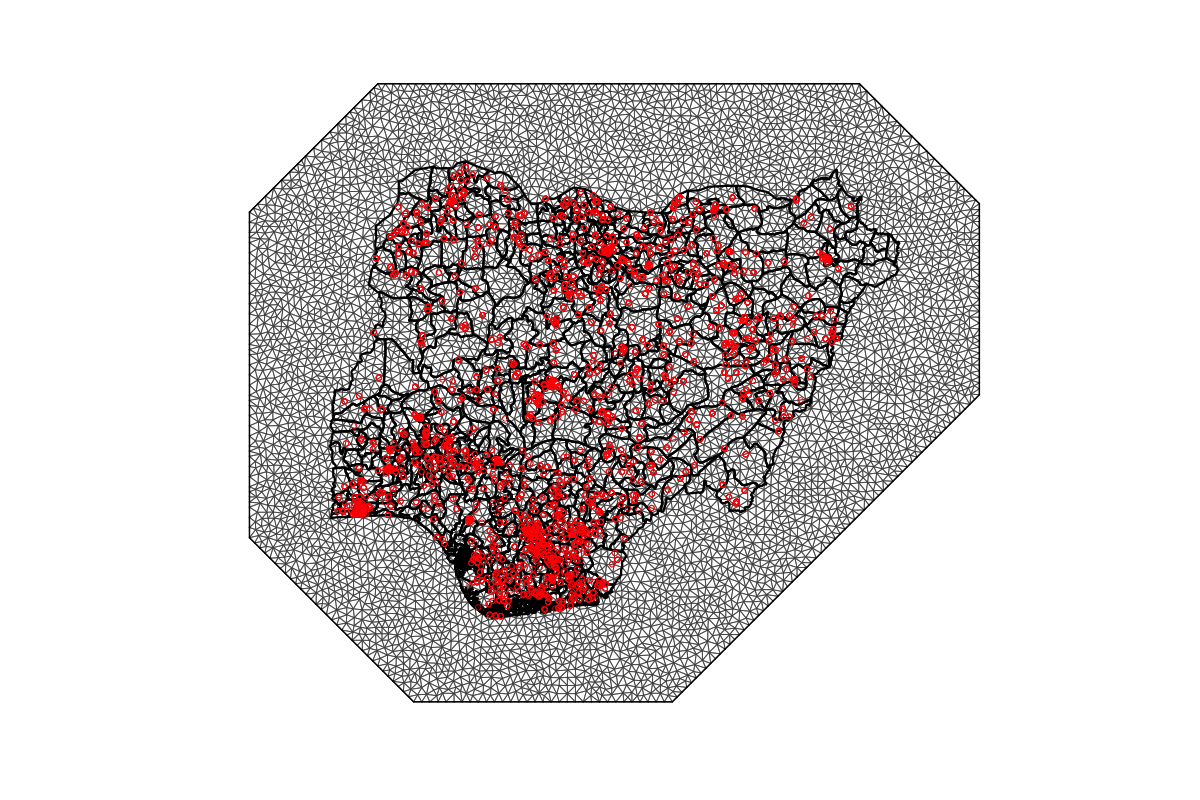
Figure A.3: Mesh used for the SPDE approach. There are 6888 vertexes and the red circles show the locations of the observed clusters.

A.6 Computing scores

Let $p_{a}$ denote the prevalence in area $a$. We consider two scoring strategies: scoring areal estimates and scoring cluster predictions.

A.6.1 Scoring admin1 estimates

We follow Section A.4, and assume that the direct estimators have the sampling distribution $\widehat{\text{logit}(p_{a})}\sim\mathcal{N}(\text{logit}(p_{a}),\hat{V}_{a})$, where $\hat{V}_{a}$ is the direct estimate of the variance. If we hold out area $b$ when estimating the model, the posterior $\pi(p_{b}|\text{Data excluding area $b$})$ is independent of $\widehat{\text{logit}(p_{b})}$ because they are based on independent data.

Let $h_{b}$ be the observed value of $\widehat{\text{logit}(p_{b})}$, then we can view $h_{b}$ as a noisy observation of the true value $\text{logit}(p_{b})$. The key observation is that if we combine the independent sampling distribution of the direct estimator with the model-based posterior for the true value $\text{logit}(p_{b})$, we find a predictive distribution $\pi(h_{b}|\text{Data excluding area $b$})$. This allows us to directly score performance for estimation of areal prevalences. The discriminatory power of this approach depends on the size of $\hat{V}_{b}$ versus the sharpness of the model-based posteriors.

Use $H_{b}$ to denote the stochastic variable, and $h_{b}$ to be the observed value. We compute two scores:

• MSE:

  $$\text{MSE}=\frac{1}{37}\sum_{b=1}^{37}(h_{b}-\mathrm{median}[H_{b}|\text{``Data excluding area $b$''}])^{2}.$$

• LogScore:

  $$\text{LogScore}=\frac{1}{37}\sum_{b=1}^{37}-\log(\pi(H_{b}=h_{b}|\text{``Data excluding area $b$''})).$$

The negative sign in the log-score ensures that lower is better for both MSE and LogScore.

A.6.2 Scoring cluster predictions

Cluster predictions are scored in a standard way through 10-fold cross validation. The clusters are randomly divided into 10 folds, each fold is held out in turn, and the response in the hold-out clusters is predicted. Scores are computed by comparing the observed proportion of vaccinated children with predicted proportion of vaccinated children. We compute both MSE and the log-score averaged over all clusters.

A.7 Diagnostics: sharing effect of urban/rural

All models use the assumption that we can use the same effect of urban versus rural in all 37 admin1 areas. We investigate this assumption by modifying UL-Int-Cov to use 37 separate coefficients of urban versus rural $\beta_{a}$, $a=1,\ldots,37$. Figure A.4 demonstrates that this assumption is not unreasonable given the amount of information available in the data. The large mismatch for $a=25$ is because everyone was vaccinated in the rural part of area $a=25$, and should be ignored.

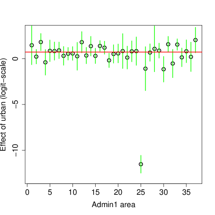
Figure A.4: Estimated effects $\beta_{a}$ of urban versus rural for admin1 areas $a=1,\ldots,37$. The green lines show 95% credible intervals. Note that estimation breaks down for area 25 to observing everyone vaccinated in the rural part of the area. The red line shows the corresponding estimate when $\beta_{1}=\cdots=\beta_{37}$.

A.8 Comparison of admin1 estimates

The MCV1 coverage estimates for the admin1 areas for direct estimates and area-level models are shown in Figure A.5, unit-level models without spatial effects and admin1 spatial effects are shown in Figure A.6, and unit-level models with admin2 spatial effects and GRFs are shown in Figure A.7. The only striking difference is that UL-Int and UL-Int-Cov seems to be missing most of the spatial variation, and that there is higher attenuation in the estimates as we model at finer and finer spatial scales.

The coefficients of variations for the MCV1 coverage estimates for the admin1 areas for direct estimates and area-level models are shown in Figure A.8, unit-level models without spatial effects and admin1 spatial effects are shown in Figure A.9, and unit-level models with admin2 spatial effects and GRFs are shown in Figure A.10. For UL-Int and UL-Int-Cov the uncertainty is unrealistically low, there is a clear reduction in uncertainty when moving from direct estimates and area-level models to unit-level models, and uncertainty reduces as we model at finer and finer spatial scales in the unit-level models.

(a) DE-Weighted.

(b) FH-IID.

(c) FH-IID-Cov.

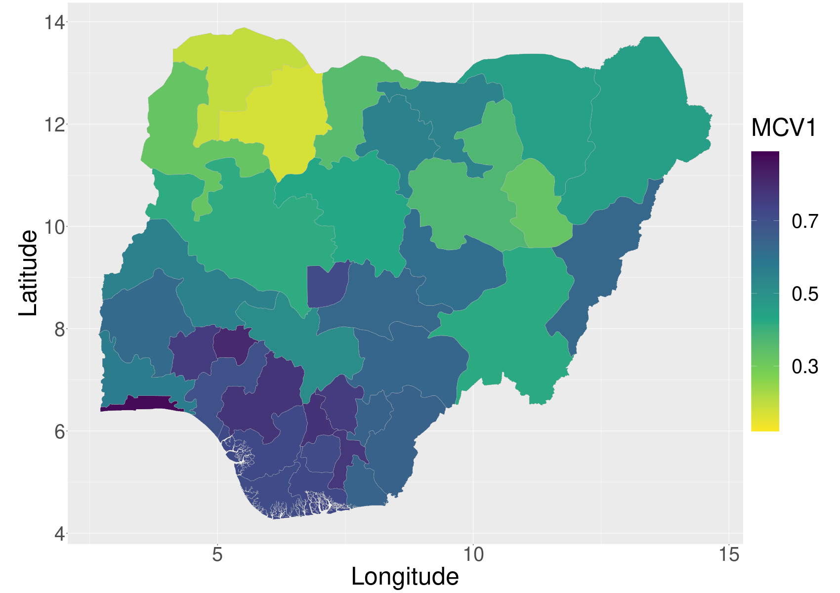
(d) FH-BYM.

(e) FH-BYM-Cov.

Figure A.5: MCV1 estimates for admin1 areas using direct estimates and area-level models.

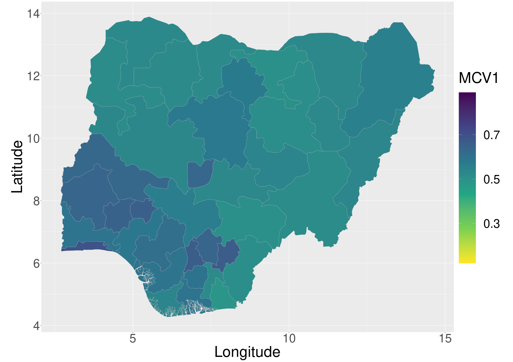
(a) UL-Int.

(b) UL-Int-Cov.

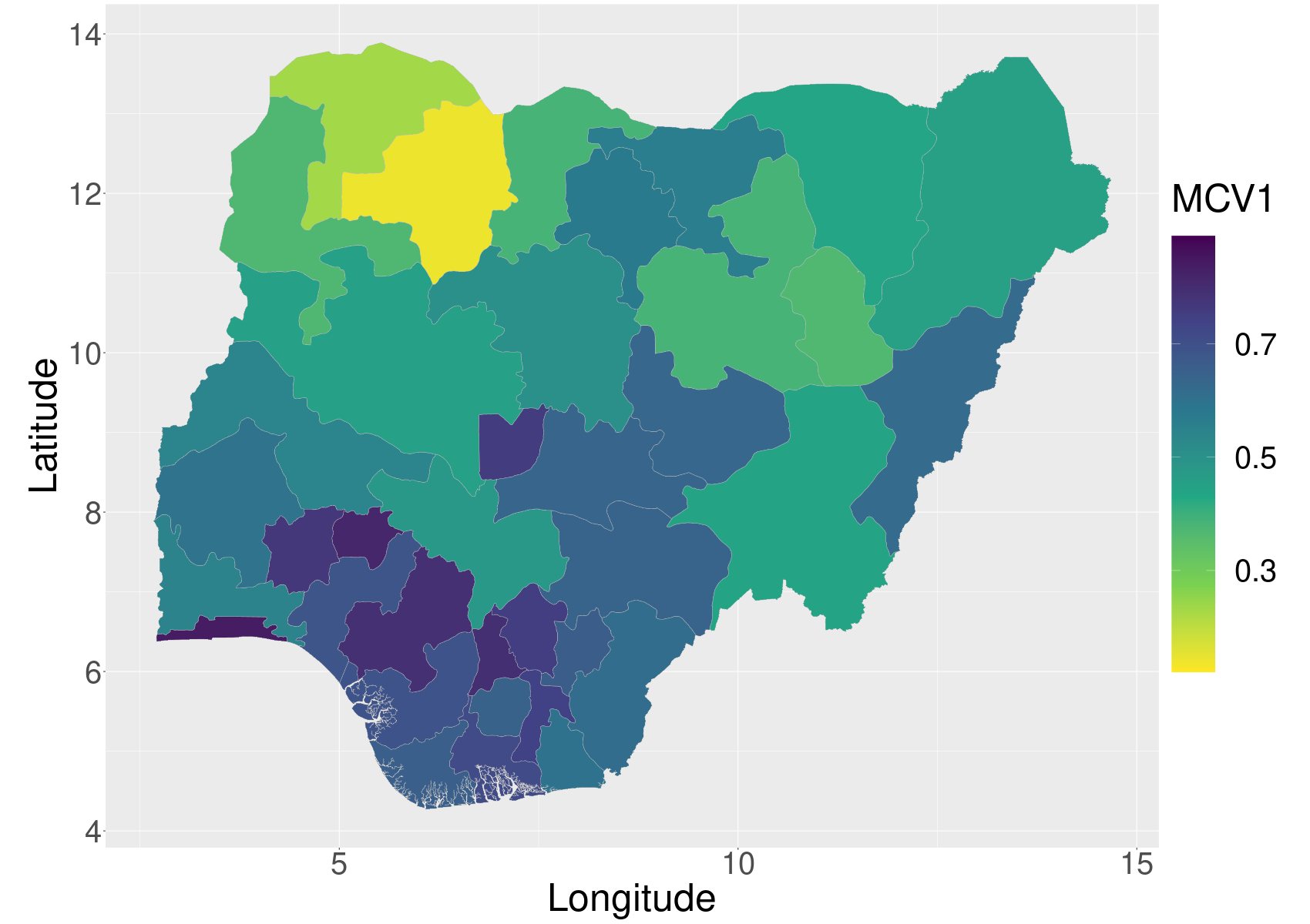
(c) UL-IID(A1).

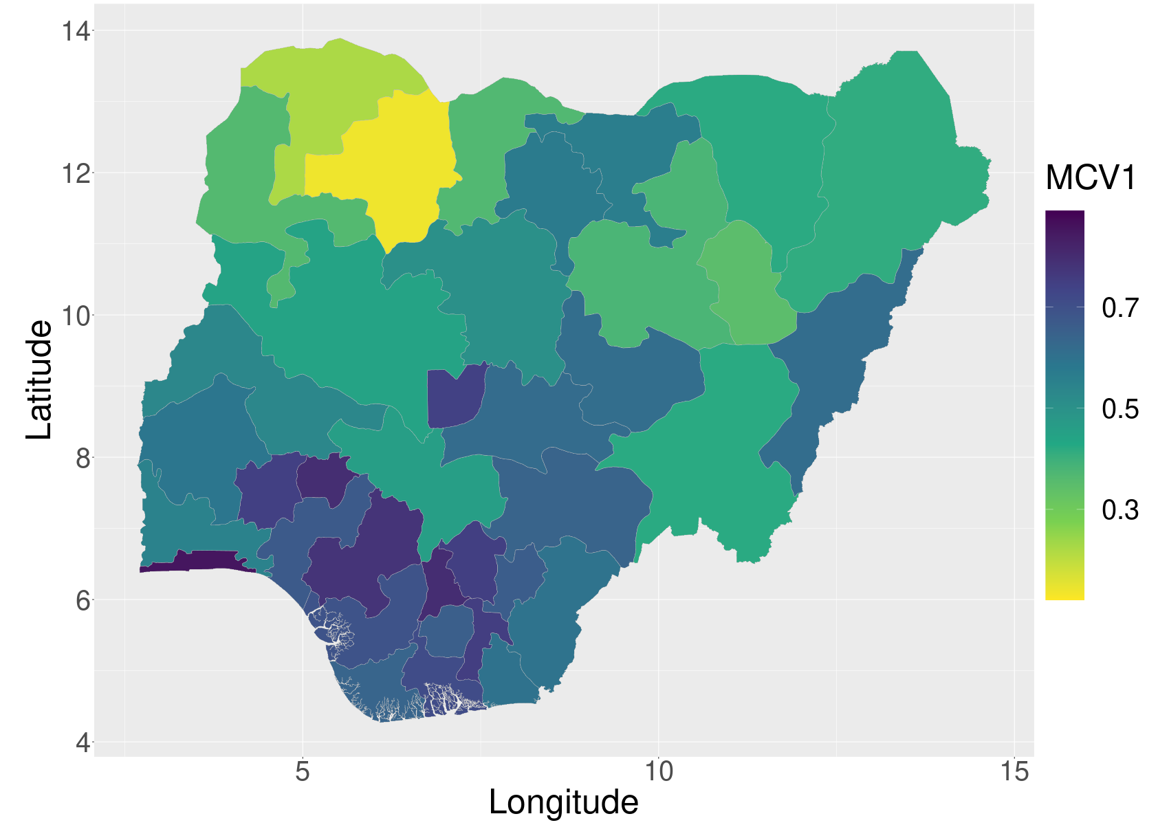
(d) UL-IID(A1)-Cov.

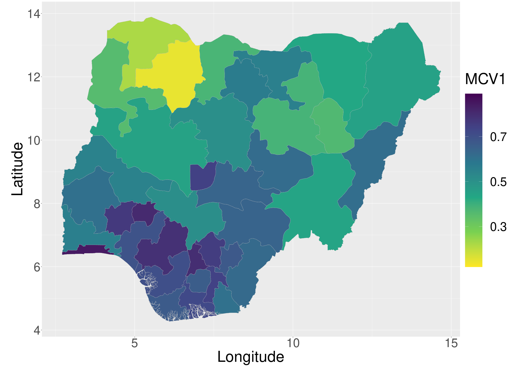
(e) UL-BYM(A1).

(f) UL-BYM(A1)-Cov.

Figure A.6: MCV1 estimates for admin1 areas using unit-level models without random effects or random effects at admin1.

(a) UL-BYM(A2).

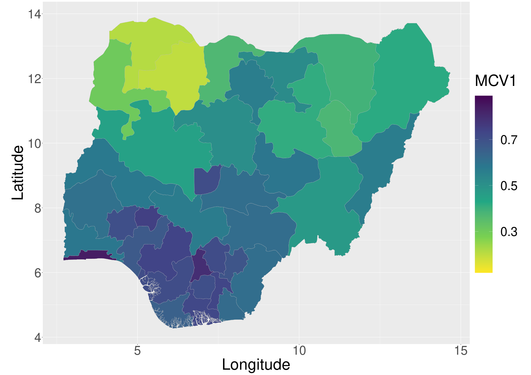
(b) UL-BYM(A2)-Cov.

(c) UL-GRF.

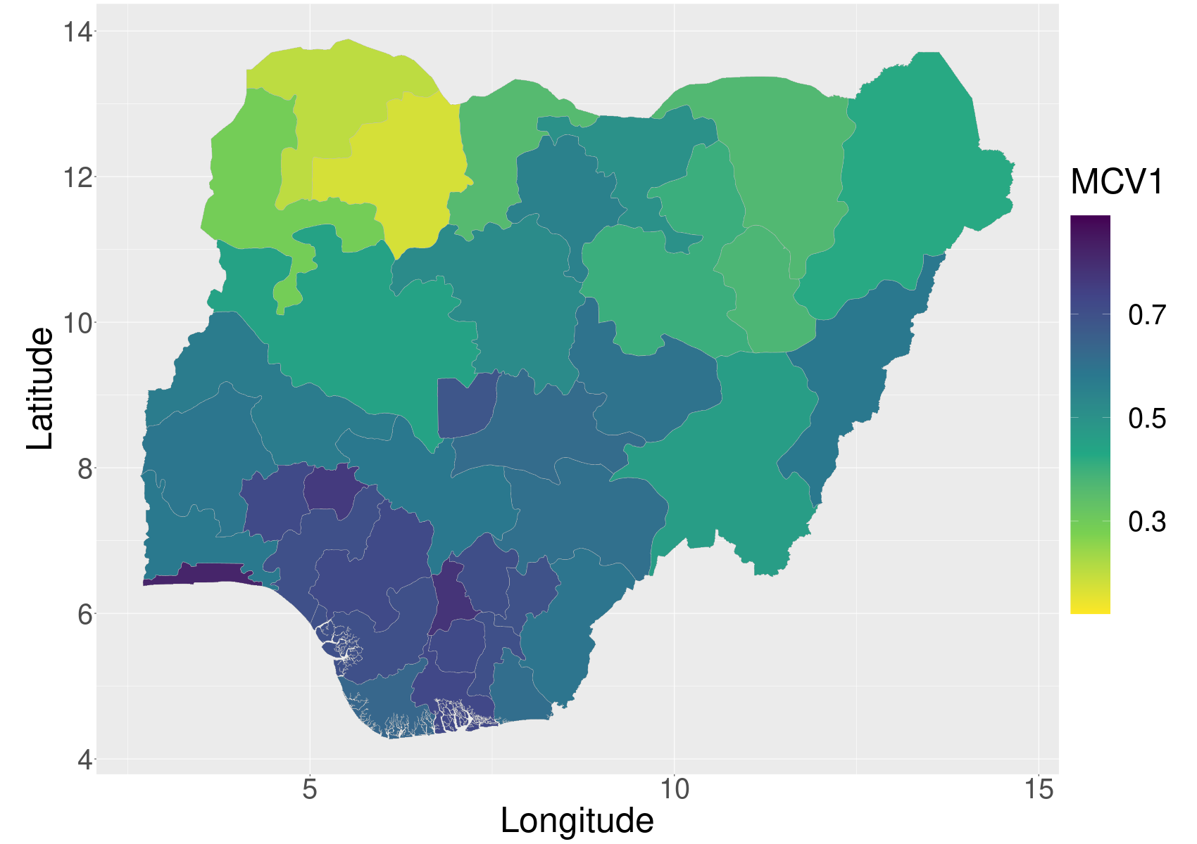
(d) UL-GRF-Cov.

Figure A.7: MCV1 estimates for admin1 areas using unit-level models with random effects at admin2 or a continuous space GRF.

(a) DE-Weighted.

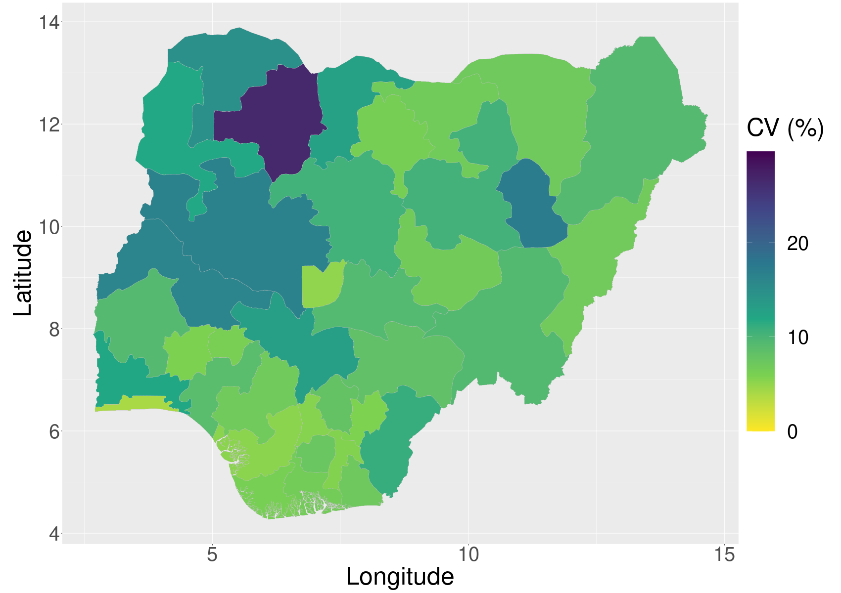
(b) FH-IID.

(c) FH-IID-Cov.

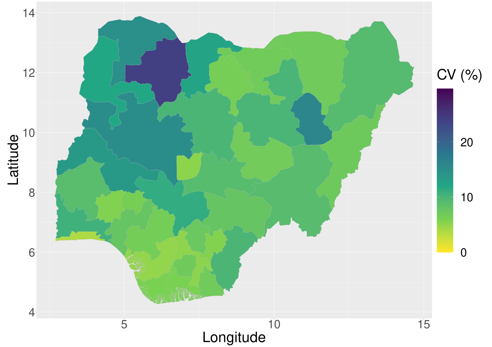
(d) FH-BYM.

(e) FH-BYM-Cov.

Figure A.8: Coefficients of variations for MCV1 estimates for admin1 areas using direct estimates and area-level models.

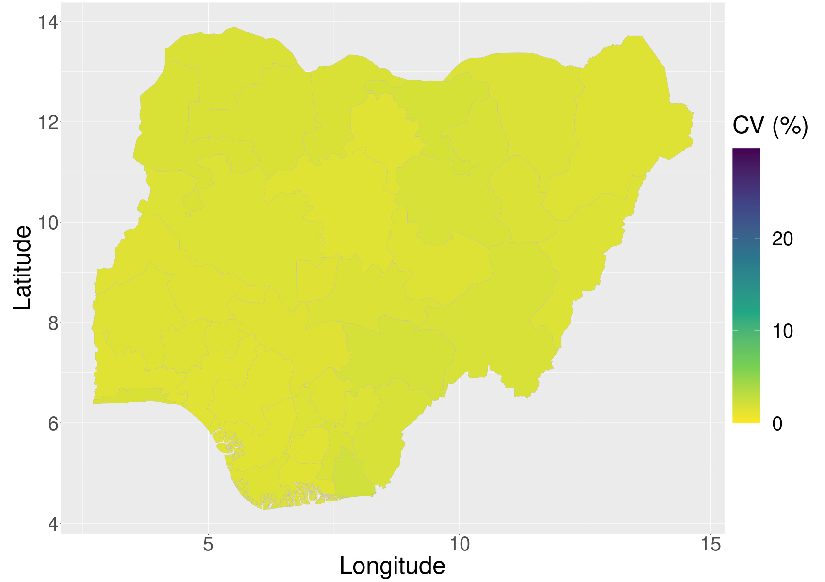
(a) UL-Int.

(b) UL-Int-Cov.

(c) UL-IID(A1).

(d) UL-IID(A1)-Cov.

(e) UL-BYM(A1).

(f) UL-BYM(A1)-Cov.

Figure A.9: Coefficients of variations for MCV1 estimates for admin1 areas using unit-level models without random effects or random effects at admin1.

(a) UL-BYM(A2).

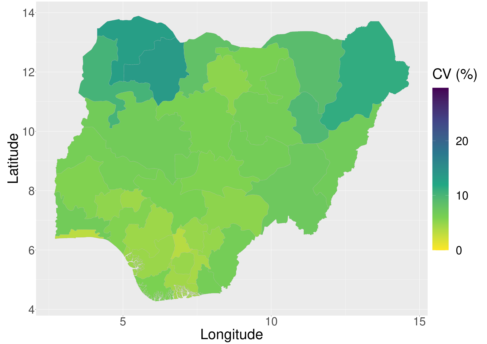
(b) UL-BYM(A2)-Cov.

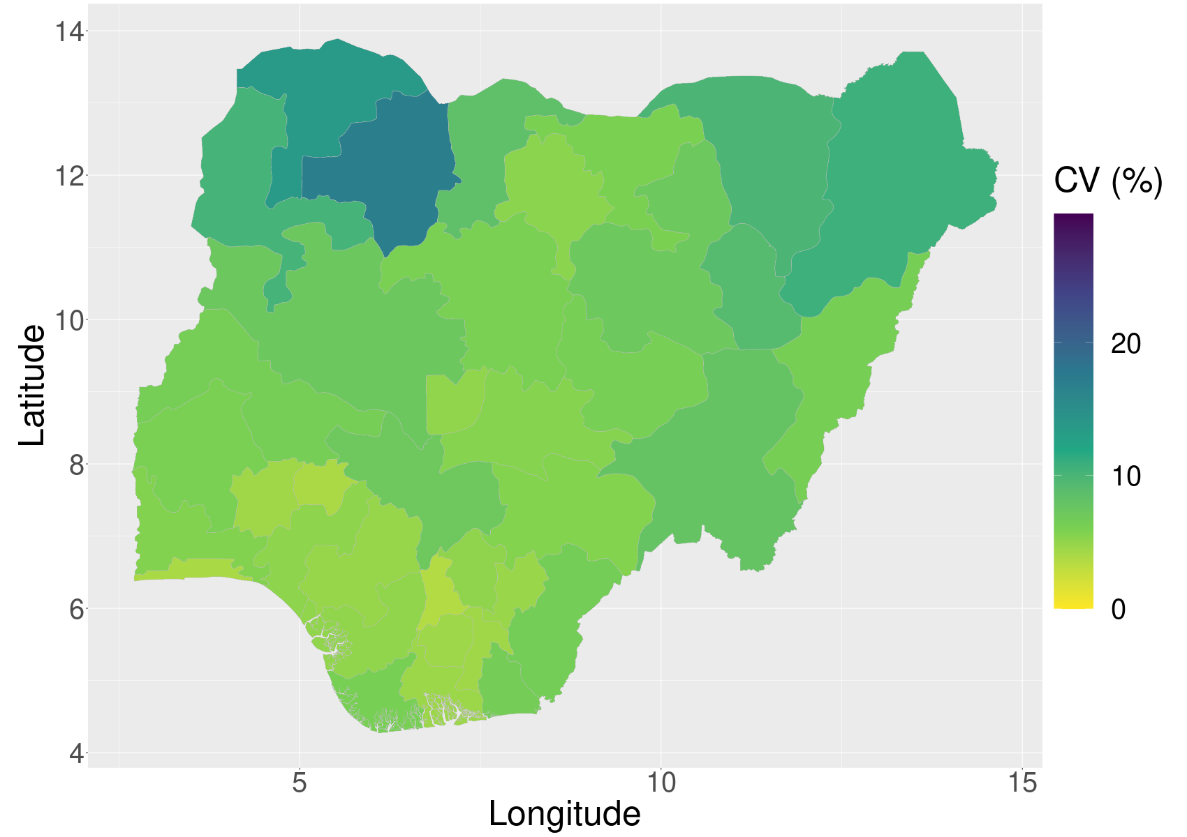
(c) UL-GRF.

(d) UL-GRF-Cov.

Figure A.10: Coefficients of variations for MCV1 estimates for admin1 areas using unit-level models with random effects at admin2 or a continuous space GRF.

A.9 Comparison of admin2 estimates

The MCV1 coverage estimates for the admin2 areas for unit-level models without spatial effects and admin1 spatial effects are shown in Figure A.11, and unit-level models with admin2 spatial effects and GRFs are shown in Figure A.12. UL-Int and UL-Int-Cov does not capture the spatial variation observed in the other models, and the models with a spatial effect at admin1 resolution does not estimate much variation within each admin1. UL-BYM(A2) and UL-BYM(A2)-Cov is similar to UL-GRF and UL-GRF-Cov, but the former shows much more noisy behaviour than the latter.

The coefficients of variations for the MCV1 coverage estimates for the admin2 areas for unit-level models without spatial effects and admin1 spatial effects are shown in Figure A.13, and unit-level models with admin2 spatial effects and GRFs are shown in Figure A.14. For UL-Int and UL-Int-Cov, the uncertainty is unrealistically low. The uncertainty in the estimates is highest when modelling at finer spatial scale, and the highest uncertainty is observed for UL-BYM(A2) and UL-BYM(A2)-Cov.

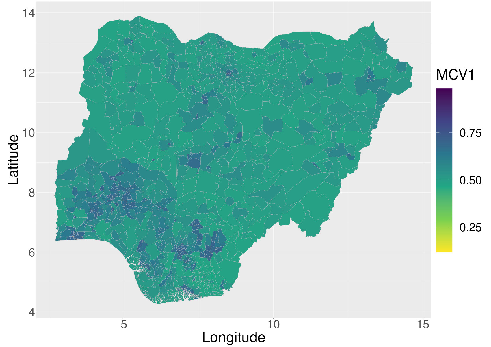
(a) UL-Int.

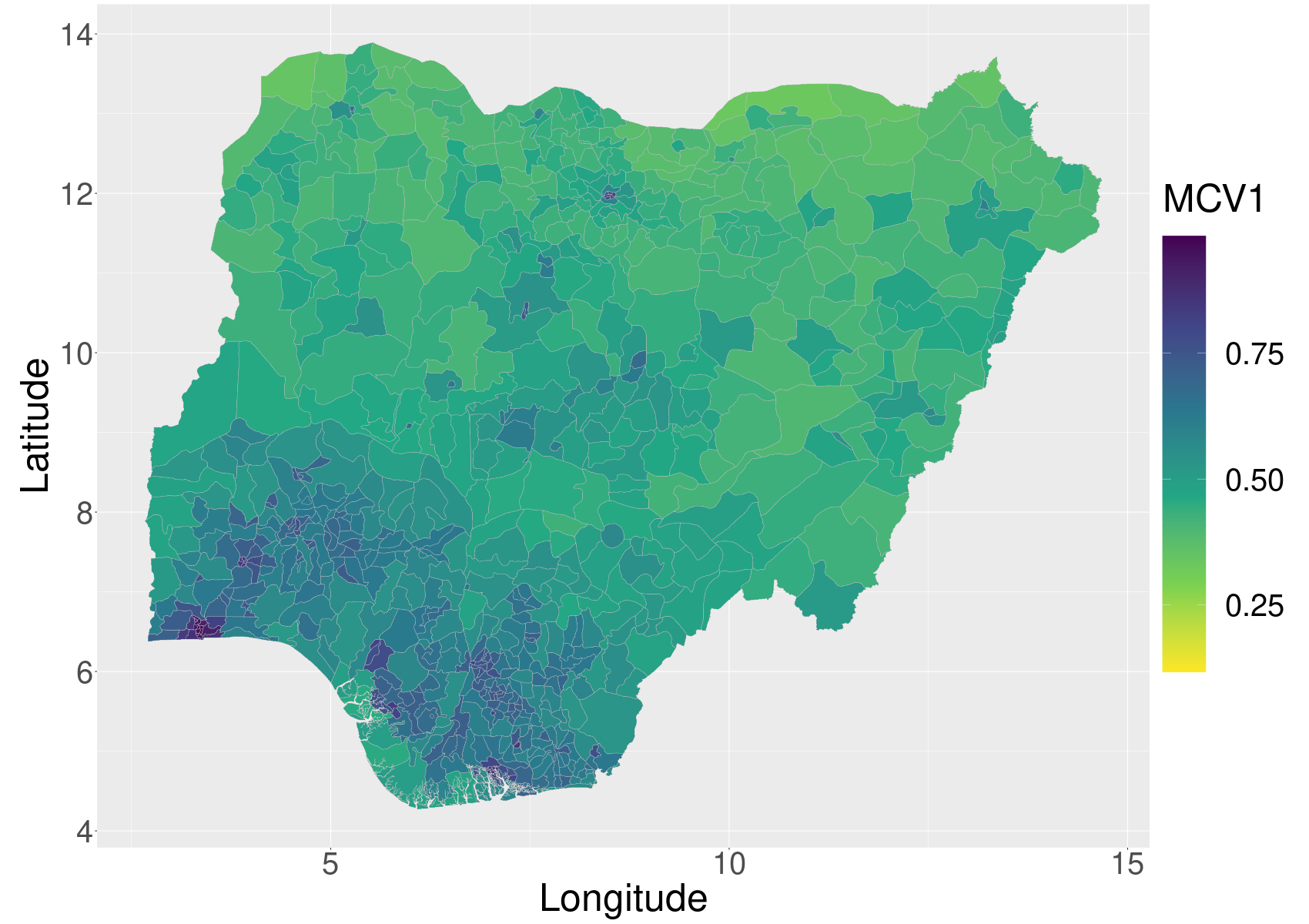
(b) UL-Int-Cov.

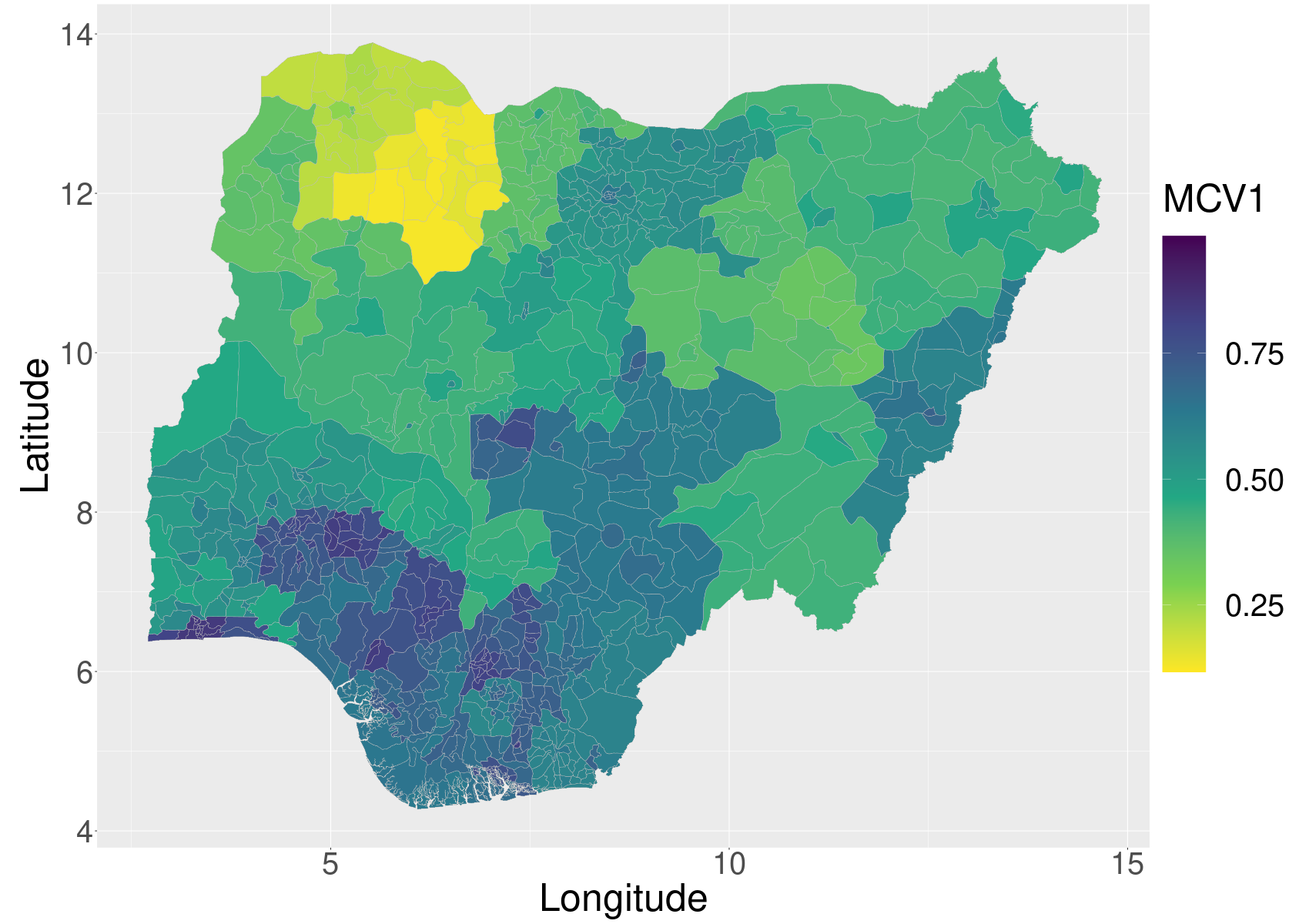
(c) UL-IID(A1).

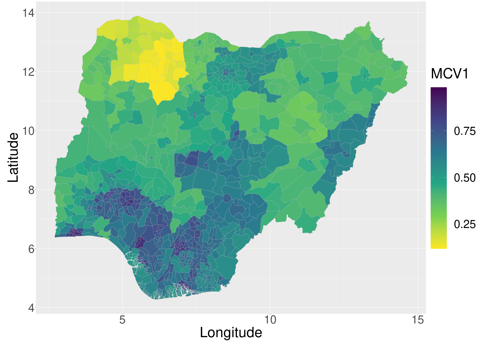
(d) UL-IID(A1)-Cov.

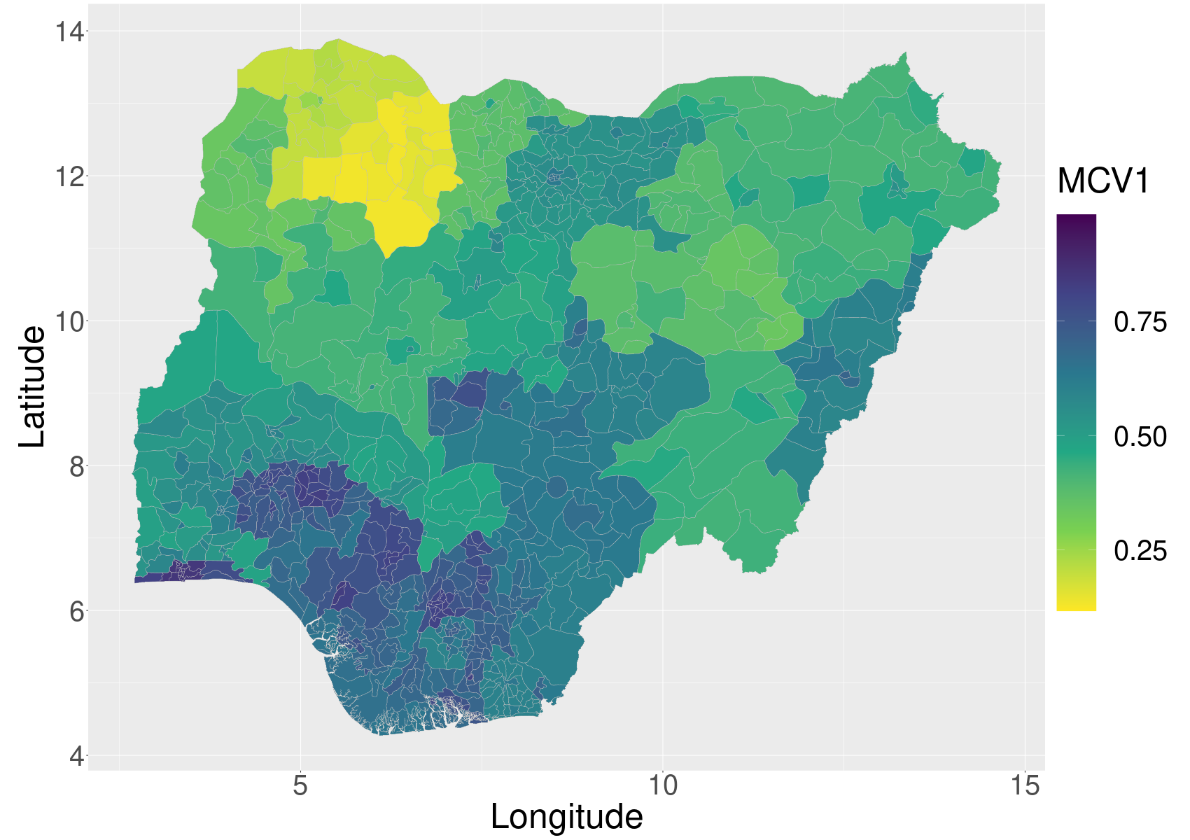
(e) UL-BYM(A1).

(f) UL-BYM(A1)-Cov.

Figure A.11: MCV1 estimates for admin2 areas using unit-level models without random effects or random effects at admin1.

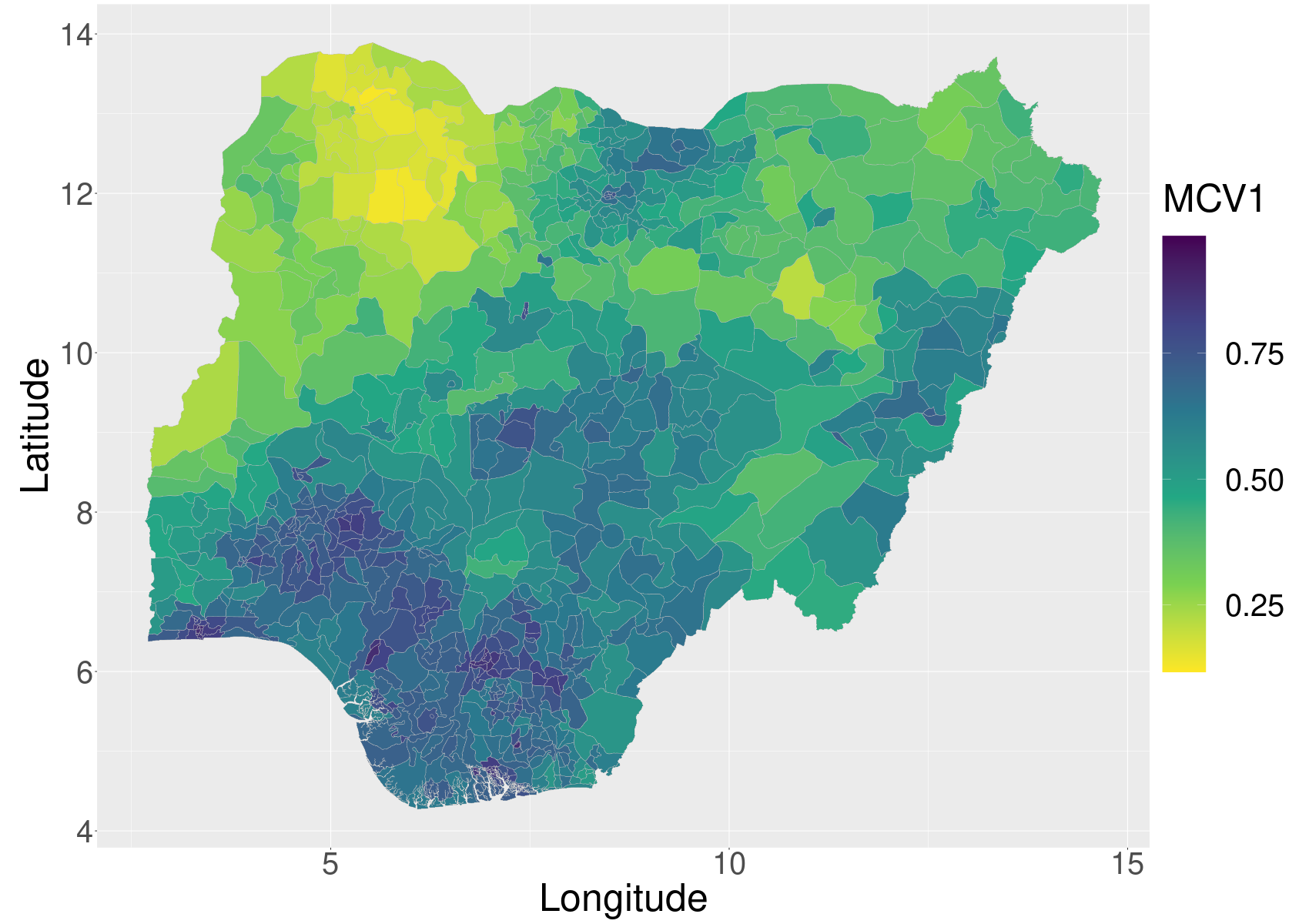
(a) UL-BYM(A2).

(b) UL-BYM(A2)-Cov.

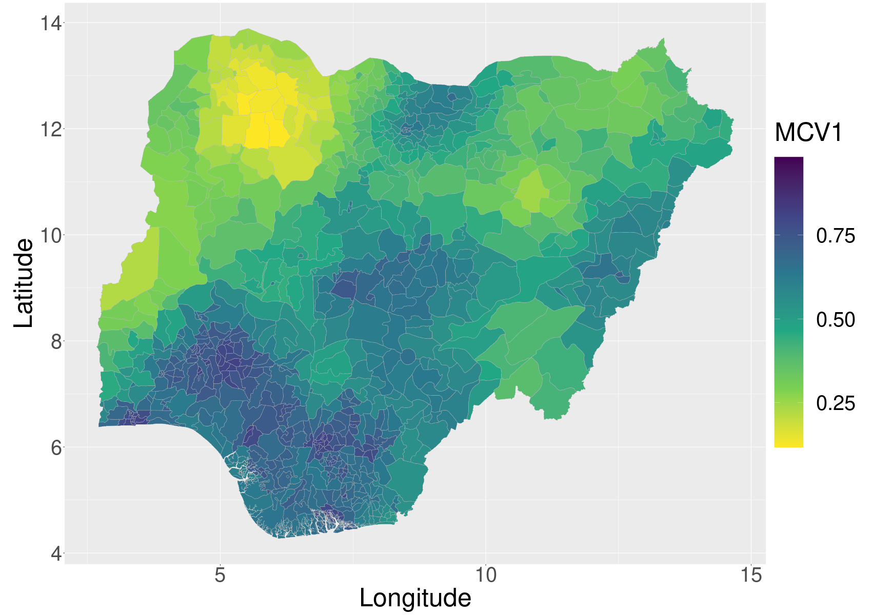
(c) UL-GRF.

(d) UL-GRF-Cov.

Figure A.12: MCV1 estimates for admin2 areas using unit-level models with random effects at admin2 or a continuous space GRF.

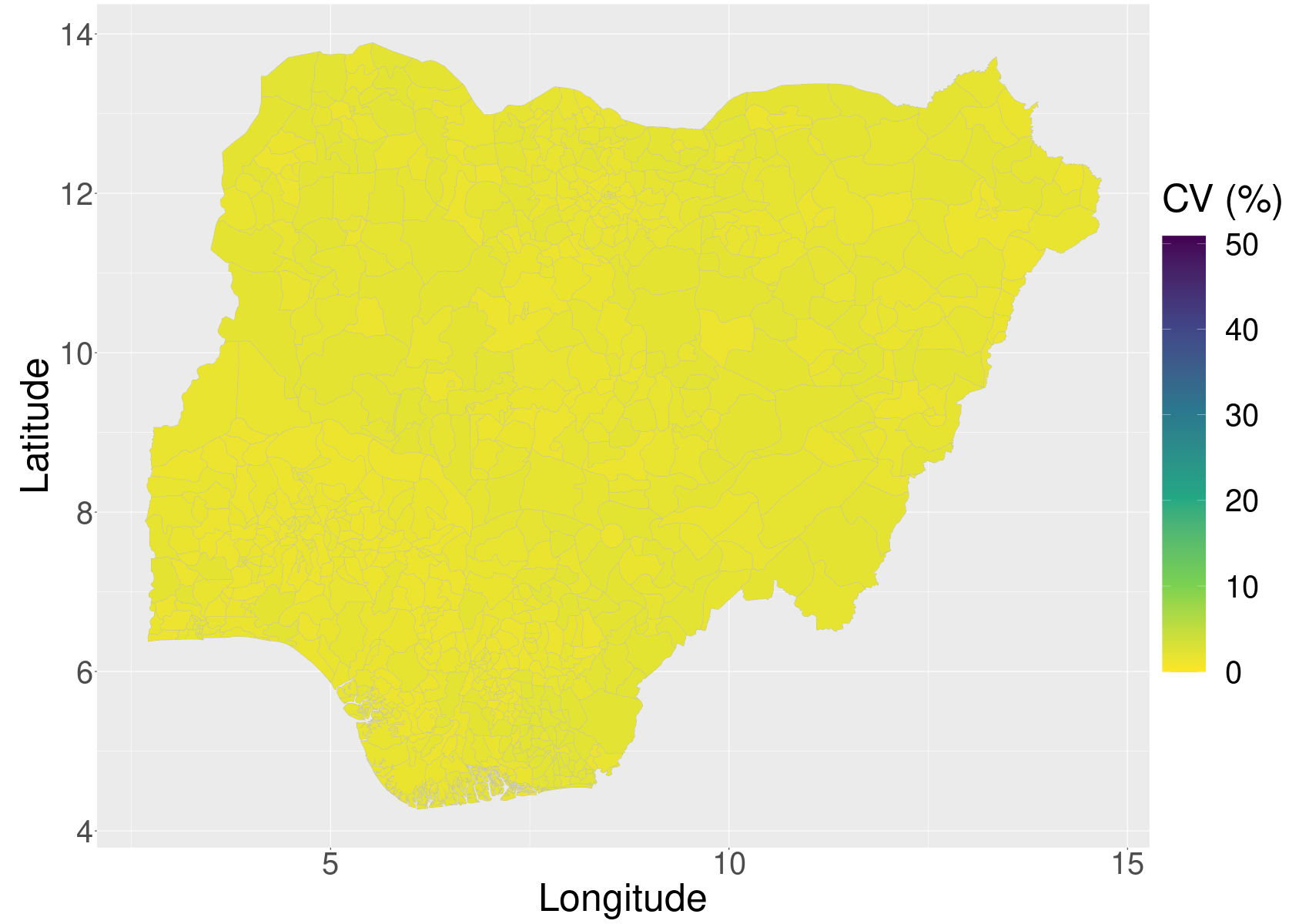
(a) UL-Int.

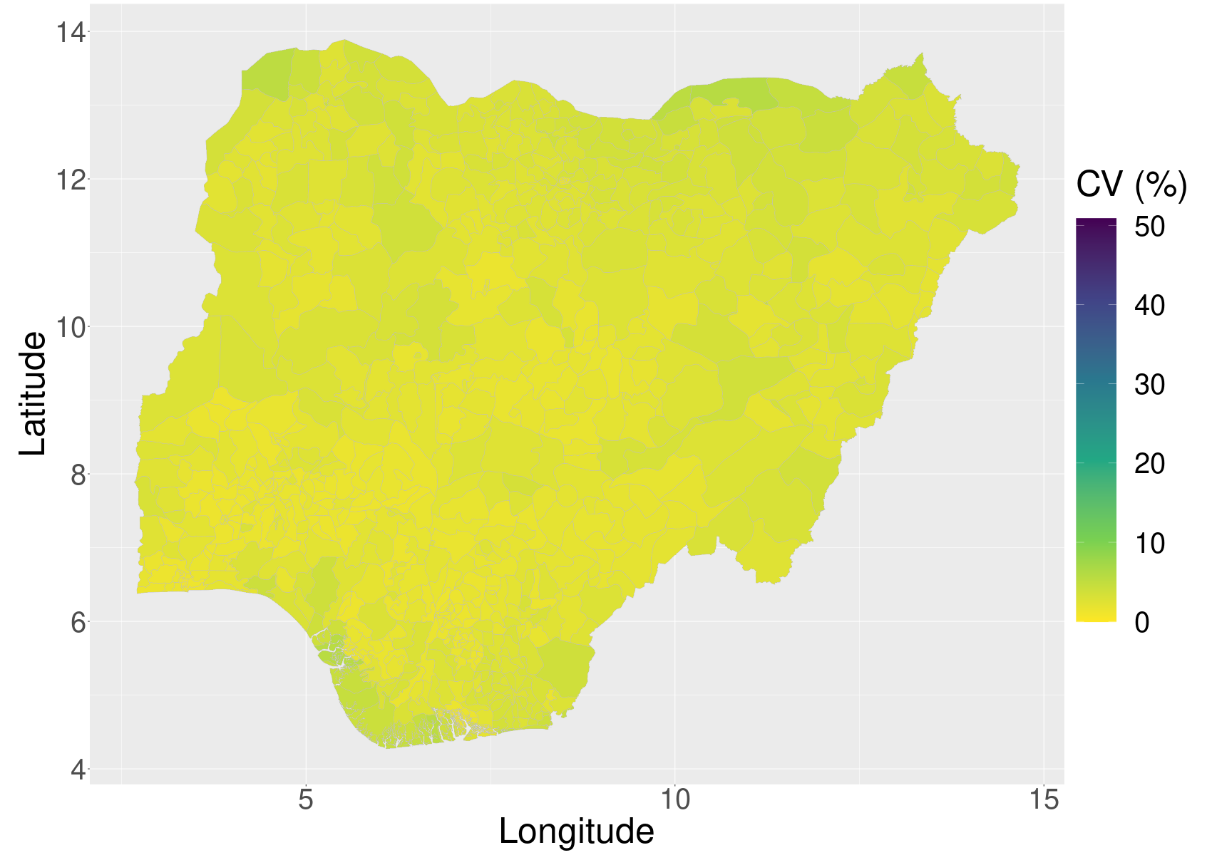
(b) UL-Int-Cov.

(c) UL-IID(A1).

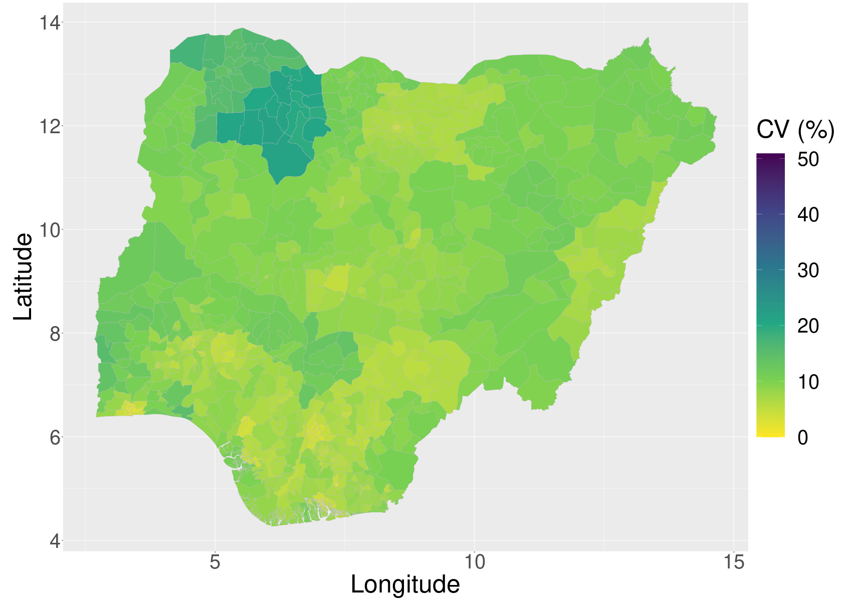
(d) UL-IID(A1)-Cov.

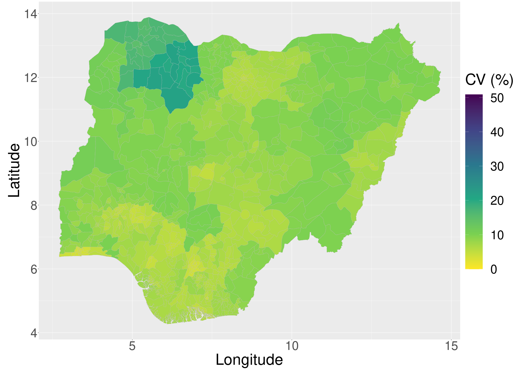
(e) UL-BYM(A1).

(f) UL-BYM(A1)-Cov.

Figure A.13: Coefficients of variations for MCV1 estimates for admin2 areas using unit-level models without random effects or random effects at admin1.

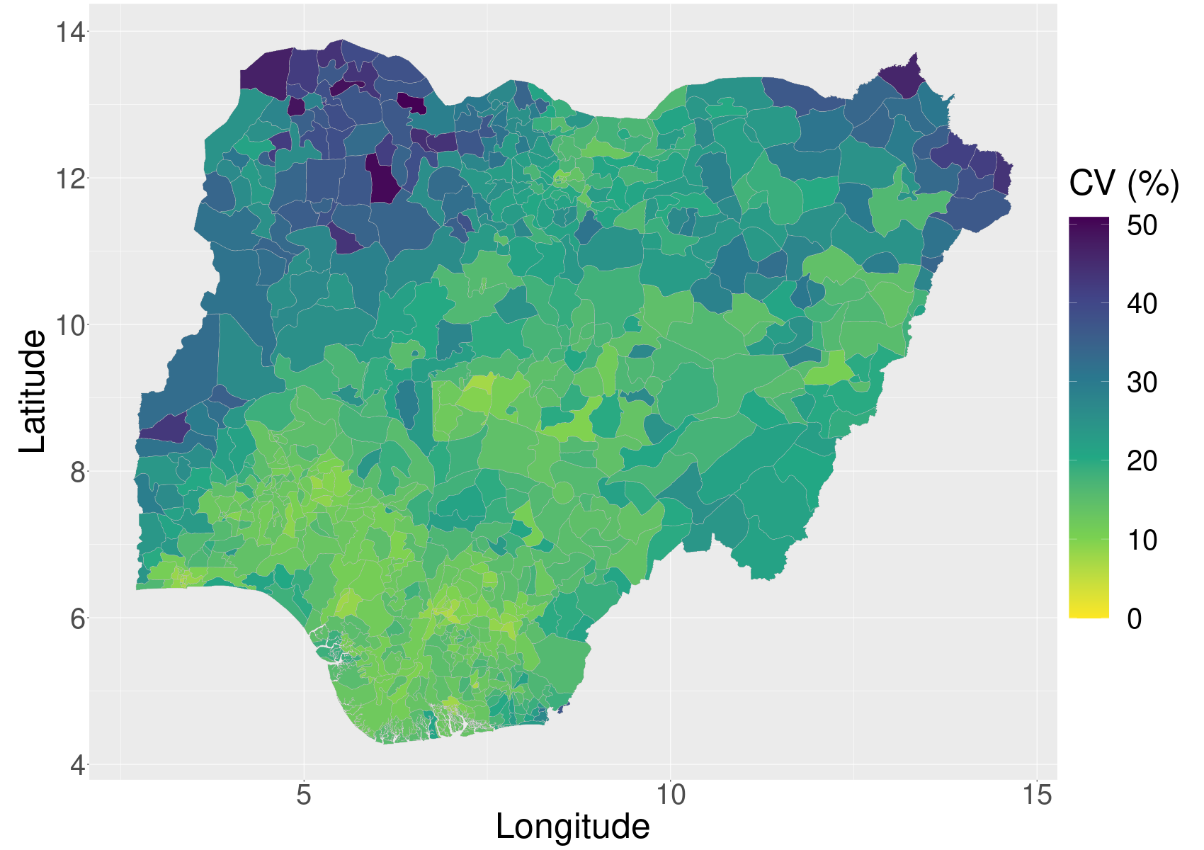
(a) UL-BYM(A2).

(b) UL-BYM(A2)-Cov.

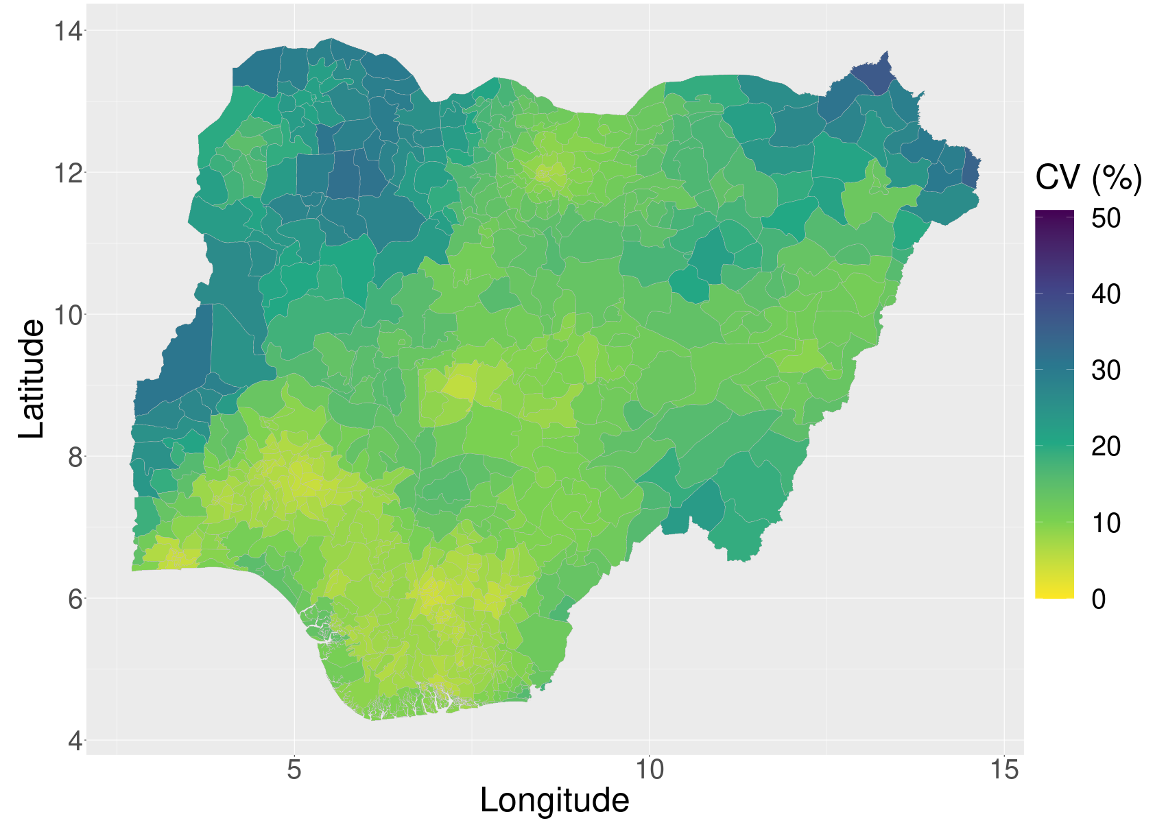
(c) UL-GRF.

(d) UL-GRF-Cov.

Figure A.14: Coefficients of variations for MCV1 estimates for admin1 areas using unit-level models with random effects at admin2 or a continuous space GRF.

References

- Bakka et al., (2018) Bakka, H., Rue, H., Fuglstad, G.-A., Riebler, A., Bolin, D., Illian, J., Krainski, E., Simpson, D., and Lindgren, F. (2018). Spatial modeling with r-inla: A review. WIREs Computational Statistics, 10:e1443.
- Battese et al., (1988) Battese, G. E., Harter, R. M., and Fuller, W. A. (1988). An error-components model for prediction of county crop areas using survey and satellite data. Journal of the American Statistical Association, 83:28–36.
- Bell et al., (2016) Bell, W. R., Basel, W., and Maples, J. (2016). An overview of the US Census Bureau’s small area income and poverty estimates program. In Pratesi, M., editor, Analysis of Poverty Data by Small Area Estimation, pages 349–378. Wiley Online Library.
- Besag, (1974) Besag, J. (1974). Spatial interaction and the statistical analysis of lattice systems. Journal of the Royal Statistical Society, Series B, 36:192–236.
- Breidt and Opsomer, (2017) Breidt, J. and Opsomer, J. (2017). Model-assisted survey estimation with modern prediction techniques. Statistical Science.
- Burstein et al., (2019) Burstein, R., Henry, N. J., Collison, M. L., Marczak, L. B., Sligar, A., Watson, S., Marquez, N., Abbasalizad-Farhangi, M., Abbasi, M., Abd-Allah, F., et al. (2019). Mapping 123 million neonatal, infant and child deaths between 2000 and 2017. Nature, 574:353–358.
- Burstein et al., (2018) Burstein, R., Wang, H., Reiner Jr, R. C., and Hay, S. I. (2018). Development and validation of a new method for indirect estimation of neonatal, infant, and child mortality trends using summary birth histories. PLoS Medicine, 15:e1002687.
- Chung and Datta, (2020) Chung, H. C. and Datta, G. S. (2020). Bayesian hierarchical spatial models for small area estimation. Technical report, Center for Statistical Research & Methodology, U.S. Census Bureau.
- Corral et al., (2021) Corral, P., Himelein, K., McGee, K., and Molina, I. (2021). A map of the poor or a poor map? Policy Research Working Paper;No. 9620, World Bank, Washington, DC.
- Cressie and Wikle, (2011) Cressie, N. and Wikle, C. (2011). Statistics for Spatio-Temporal Data. John Wiley and Sons.
- Datta et al., (2011) Datta, G. S., Kubokawa, T., Molina, I., and Rao, J. (2011). Estimation of mean squared error of model-based small area estimators. Test, 20:367–388.
- Diggle and Giorgi, (2016) Diggle, P. and Giorgi, E. (2016). Model-based geostatistics for prevalence mapping in low-resource settings. Journal of the American Statistical Association, 111:1096–1120.
- Diggle and Giorgi, (2019) Diggle, P. J. and Giorgi, E. (2019). Model-based Geostatistics for Global Public Health: Methods and Applications. Chapman and Hall/CRC, Boca-Raton.
- Diggle et al., (2010) Diggle, P. J., Menezes, R., and Su, T.-L. (2010). Geostatistical inference under preferential sampling. Journal of the Royal Statistical Society: Series C, 59:191–232.
- Dong and Wakefield, (2021) Dong, T. and Wakefield, J. (2021). Modeling and presentation of health and demographic indicators in a low- and middle-income countries context. Vaccine, 39:2584–2594.
- Fay and Herriot, (1979) Fay, R. and Herriot, R. (1979). Estimates of income for small places: an application of James–Stein procedure to census data. Journal of the American Statistical Association, 74:269–277.
- Fuglstad et al., (2019) Fuglstad, G.-A., Simpson, D., Lindgren, F., and Rue, H. (2019). Constructing priors that penalize the complexity of Gaussian random fields. Journal of the American Statistical Association, 114:445–452.
- Gelfand, (2010) Gelfand, A. (2010). Misaligned spatial data. In Gelfand, A., Diggle, P., Fuentes, M., and Guttorp, P., editors, Handbook of Spatial Statistics, pages 517–539. CRC Press.
- Gelman and Hill, (2006) Gelman, A. and Hill, J. (2006). Data Analysis using Regression and Multilevel/Hierarchical Models. Cambridge University Press.
- General Assembly of the United Nations, (2015) General Assembly of the United Nations (2015). Resolution adopted by the General Assembly on 25 September 2015. A/RES/70/1.
- Giorgi and Diggle, (2017) Giorgi, E. and Diggle, P. J. (2017). Prevmap: An r package for prevalence mapping. Journal of Statistical Software, Articles, 78:1–29.
- Golding et al., (2017) Golding, N., Burstein, R., Longbottom, J., Browne, A., Fullman, N., Osgood-Zimmerman, A., Earl, L., Bhatt, S., Cameron, E., Casey, D., Dwyer-Lindgren, L., Farag, T., Flaxman, A., Fraser, M., Gething, P., Gibson, H., Graetz, N., Krause, L., Kulikoff, X., Lim, S., Mappin, B., Morozoff, C., Reiner, R., Sligar, A., Smith, D., Wang, H., Weiss, D., Murray, C., Moyes, C., and Hay, S. (2017). Mapping under-5 and neontal mortality in Africa, 2000–15: a baseline analysis for the Sustainable Development Goals. The Lancet, 390:2171–2182.
- Hájek, (1971) Hájek, J. (1971). Discussion of, “An essay on the logical foundations of survey sampling, part I”, by D. Basu. In Godambe, V. and Sprott, D., editors, Foundations of Statistical Inference. Holt, Rinehart and Winston, Toronto.
- Horvitz and Thompson, (1952) Horvitz, D. and Thompson, D. (1952). A generalization of sampling without replacement from a finite universe. Journal of the American Statistical Association, 47:663–685.
- Hosseinpoor et al., (2016) Hosseinpoor, A. R., Bergen, N., Barros, A. J., Wong, K. L., Boerma, T., and Victora, C. G. (2016). Monitoring subnational regional inequalities in health: measurement approaches and challenges. International Journal for Equity in Health, 15:1–13.
- ICF International, (2012) ICF International (2012). Demographic and Health Survey Samling and Household Listing Manual. MEASURE DHS, MD: Claverton.
- Kristensen et al., (2016) Kristensen, K., Nielsen, A., Berg, C. W., Skaug, H., and Bell, B. M. (2016). TMB: Automatic differentiation and laplace approximation. Journal of Statistical Software, Articles, 70:1–21.
- Lehtonen and Veijanen, (2009) Lehtonen, R. and Veijanen, A. (2009). Design-based methods of estimation for domains and small areas. In Handbook of statistics, volume 29, pages 219–249. Elsevier.
- Leroux et al., (1999) Leroux, B., Lei, X., and Breslow, N. (1999). Estimation of disease rates in small areas: A new mixed model for spatial dependence. In Halloran, M. and Berry, D., editors, Statistical Models in Epidemiology, the Environment and Clinical Trials, pages 179–192. Springer, New York.
- (30) Li, Z., Hsiao, Y., Godwin, J., Martin, B. D., Wakefield, J., Clark, S. J., with support from the United Nations Inter-agency Group for Child Mortality Estimation, and its technical advisory group (2019a). Changes in the spatial distribution of the under-five mortality rate: Small-area analysis of 122 DHS surveys in 262 subregions of 35 countries in Africa. PloS one, 14:e0210645.
- (31) Li, Z. R., Hsiao, Y., Godwin, J., Martin, B. D., Wakefield, J., and Clark, S. J. (2019b). Changes in the spatial distribution of the under five mortality rate: small-area analysis of 122 DHS surveys in 262 subregions of 35 countries in Africa. PLoS One, 14:e0210645.
- Li et al., (2021) Li, Z. R., Martin, B. D., Hsiao, Y., Godwin, J., Paige, J., Wakefield, J., Clark, S. J., Fuglstad, G.-A., and Riebler, A. (2021). SUMMER: SAE Unit/area Models and Methods for Estimation in R. R package version 1.2.0.
- Lindgren and Rue, (2015) Lindgren, F. and Rue, H. (2015). Bayesian spatial modelling with R-INLA. Journal of Statistical Software, 63:1–25.
- Lindgren et al., (2011) Lindgren, F., Rue, H., and Lindström, J. (2011). An explicit link between Gaussian fields and Gaussian Markov random fields: the stochastic differential equation approach (with discussion). Journal of the Royal Statistical Society, Series B, 73:423–498.
- Little, (2003) Little, R. J. (2003). The Bayesian approach to sample survey inference. In Analysis of survey data, pages 49–57. Wiley Online Library.
- Local Burden of Disease Vaccine Coverage Collaborators and others, (2021) Local Burden of Disease Vaccine Coverage Collaborators and others (2021). Mapping routine measles vaccination in low-and middle-income countries. Nature, 589:415.
- Lohr, (2009) Lohr, S. (2009). Sampling: Design and Analysis. Cengage Learning.
- Lumley, (2004) Lumley, T. (2004). Analysis of complex survey samples. Journal of Statistical Software, 9:1–19.
- Lumley, (2018) Lumley, T. (2018). survey: analysis of complex survey samples. R package version 3.35.
- Marhuenda et al., (2013) Marhuenda, Y., Molina, I., and Morales, D. (2013). Small area estimation with spatio-temporal Fay–Herriot models. Computational Statistics and Data Analysis, 58:308–325.
- Marquez and Wakefield, (2021) Marquez, N. and Wakefield, J. (2021). Harmonizing child mortality data at disparate geographic levels. Statistical Methods in Medical Research, 30:1187–1210.
- Mercer et al., (2015) Mercer, L., Wakefield, J., Pantazis, A., Lutambi, A., Mosanja, H., and Clark, S. (2015). Small area estimation of childhood mortality in the absence of vital registration. Annals of Applied Statistics, 9:1889–1905.
- Mosser et al., (2019) Mosser, J. F., Gagne-Maynard, W., Rao, P. C., Osgood-Zimmerman, A., Fullman, N., Graetz, N., Burstein, R., Updike, R. L., Liu, P. Y., Ray, S. E., et al. (2019). Mapping diphtheria-pertussis-tetanus vaccine coverage in africa, 2000–2016: a spatial and temporal modelling study. The Lancet, 393:1843–1855.
- National Population Commission - NPC and ICF, (2019) National Population Commission - NPC and ICF (2019). Nigeria demographic and health survey 2018 - final report. http://dhsprogram.com/pubs/pdf/FR359/FR359.pdf.
- Osgood-Zimmerman and Wakefield, (2021) Osgood-Zimmerman, A. and Wakefield, J. (2021). A statistical introduction to template model builder: A flexible tool for spatial modeling. arXiv preprint arXiv:2103.09929.
- Otto and Bell, (1995) Otto, M. C. and Bell, W. R. (1995). Sampling error modelling of poverty and income statistics for states. In American Statistical Association, Proceedings of the Section on Government Statistics, pages 160–165.
- Paige et al., (2020) Paige, J., Fuglstad, G.-A., Riebler, A., and Wakefield, J. (2020). Design- and model-based approaches to small-area estimation in a low and middle income country context: Comparisons and recommendations. Journal of Survey Statistics and Methodology. In press.
- Pfeffermann, (1993) Pfeffermann, D. (1993). The role of sampling weights when modeling survey data. International Statistical Review / Revue Internationale de Statistique, 61:317–337.
- Rao and Molina, (2015) Rao, J. and Molina, I. (2015). Small Area Estimation, Second Edition. John Wiley, New York.
- Riebler et al., (2016) Riebler, A., Sørbye, S., Simpson, D., and Rue, H. (2016). An intuitive Bayesian spatial model for disease mapping that accounts for scaling. Statistical Methods in Medical Research, 25:1145–1165.
- Rue et al., (2009) Rue, H., Martino, S., and Chopin, N. (2009). Approximate Bayesian inference for latent Gaussian models using integrated nested Laplace approximations (with discussion). Journal of the Royal Statistical Society, Series B, 71:319–392.
- Rue et al., (2017) Rue, H., Riebler, A., Sørbye, S. H., Illian, J. B., Simpson, D. P., and Lindgren, F. K. (2017). Bayesian computing with inla: A review. Annual Review of Statistics and Its Application, 4:395–421.
- Särndal, (2007) Särndal, C.-E. (2007). The calibration approach in survey theory and practice. Survey Methodology, 33:99–119.
- Scott and Smith, (1969) Scott, A. and Smith, T. (1969). Estimation in multi-stage surveys. Journal of the American Statistical Association, 64:830–840.
- Simpson et al., (2017) Simpson, D., Rue, H., Riebler, A., Martins, T., and Sørbye, S. (2017). Penalising model component complexity: A principled, practical approach to constructing priors (with discussion). Statistical Science, 32:1–28.
- Sørbye and Rue, (2014) Sørbye, S. and Rue, H. (2014). Scaling intrinsic Gaussian Markov random field priors in spatial modelling. Spatial Statistics, 8:39–51.
- Stevens et al., (2016) Stevens, G. A., Alkema, L., Black, R. E., Boerma, J. T., Collins, G. S., Ezzati, M., Grove, J. T., Hogan, D. R., Hogan, M. C., Horton, R., et al. (2016). Guidelines for accurate and transparent health estimates reporting: the GATHER statement. PLoS medicine, 13:e1002056.
- Sugden and Smith, (1984) Sugden, R. A. and Smith, T. M. F. (1984). Ignorable and informative designs in survey sampling inference. Biometrika, 71:495–506.
- Sørbye and Rue, (2017) Sørbye, S. H. and Rue, H. (2017). Penalised complexity priors for stationary autoregressive processes. Journal of Time Series Analysis, 38:923–935.
- Takahashi et al., (2017) Takahashi, S., Metcalf, C. J. E., Ferrari, M. J., Tatem, A. J., and Lessler, J. (2017). The geography of measles vaccination in the african great lakes region. Nature communications, 8:15585.
- Tatem et al., (2021) Tatem, A., Gething, P., Bhatt, S., Weiss, D., and Pezzulo, C. (2021). Nigeria 1km Poverty. https://www.worldpop.org/geodata/summary?id=1267. Accessed: 2021-10-18.
- Tzavidis et al., (2018) Tzavidis, N., Zhang, L.-C., Luna, A., Schmid, T., and Rojas-Perilla, N. (2018). From start to finish: a framework for the production of small area official statistics. Journal of the Royal Statistical Society, Series A, 181:927–979.
- UN IGME, (2021) UN IGME (2021). Subnational Under-five Mortality Estimates, 1990–2019: Estimates developed by the United Nations Inter-agency Group for Child Mortality Estimation. United Nations Children’s Fund, NY:New York.
- UN System Chief Executives Board for Coordination, (2017) UN System Chief Executives Board for Coordination (2017). Equality and non-discrimination at the heart of sustainable development: A shared united nations framework for action.
- Utazi et al., (2021) Utazi, C. E., Nilsen, K., Pannell, O., Dotse-Gborgbortsi, W., and Tatem, A. J. (2021). District-level estimation of vaccination coverage: Discrete vs continuous spatial models. Statistics in Medicine, 40:2197–2211.
- (66) Utazi, C. E., Thorley, J., Alegana, V. A., Ferrari, M. J., Nilsen, K., Takahashi, S., Metcalf, C. J. E., Lessler, J., and Tatem, A. J. (2018a). A spatial regression model for the disaggregation of areal unit based data to high resolution grids with application to vaccination coverage mapping. Statistical Methods in Medical Research, 28:1–16.
- Utazi et al., (2019) Utazi, C. E., Thorley, J., Alegana, V. A., Ferrari, M. J., Takahashi, S., Metcalf, C. J. E., Lessler, J., Cutts, F. T., and Tatem, A. J. (2019). Mapping vaccination coverage to explore the effects of delivery mechanisms and inform vaccination strategies. Nature communications, 10:1–10.
- (68) Utazi, C. E., Thorley, J., Alegana, V. A., Ferrari, M. J., Takahashi, S., Metcalf, C. J. E., Lessler, J., and Tatem, A. J. (2018b). High resolution age-structured mapping of childhood vaccination coverage in low and middle income countries. Vaccine, 36:1583–1591.
- Utazi et al., (2020) Utazi, C. E., Wagai, J., Pannell, O., Cutts, F. T., Rhoda, D. A., Ferrari, M. J., Dieng, B., Oteri, J., Danovaro-Holliday, M. C., Adeniran, A., et al. (2020). Geospatial variation in measles vaccine coverage through routine and campaign strategies in Nigeria: Analysis of recent household surveys. Vaccine, 38:3062–3071.
- Wakefield et al., (2019) Wakefield, J., Fuglstad, G.-A., Riebler, A., Godwin, J., Wilson, K., and Clark, S. (2019). Estimating under five mortality in space and time in a developing world context. Statistical Methods in Medical Research, 28:2614–2634.
- Watjou et al., (2017) Watjou, K., Faes, C., Lawson, A., Kirby, R., Aregay, M., Carroll, R., and Vandendijck, Y. (2017). Spatial small area smoothing models for handling survey data with nonresponse. Statistics in Medicine, 36:3708–3745.
- Weiss et al., (2018) Weiss, D. J., Nelson, A., Gibson, H., Temperley, W., Peedell, S., Lieber, A., Hancher, M., Poyart, E., Belchior, S., Fullman, N., et al. (2018). A global map of travel time to cities to assess inequalities in accessibility in 2015. Nature, 553:333–336.
- Wilson and Wakefield, (2020) Wilson, K. and Wakefield, J. (2020). Pointless spatial modeling. Biostatistics, 21:e17–e32.
- Wu et al., (2021) Wu, Y., Li, Z. R., Mayala, B., Wang, H., Gao, P., Paige, J., Fuglstad, G.-A., Moe, C., Godwin, J., Donohue, R., Janocha, B., Croft, T., and Wakefield, J. (2021). Spatial modeling for subnational administrative level 2 small-area estimation. Technical report, ICF International. DHS Spatial Analysis Reports No. 21.
- You and Rao, (2002) You, Y. and Rao, J. (2002). Small area estimation using unmatched sampling and linking models. Canadian Journal of Statistics, 30:3–15.
- You and Zhou, (2011) You, Y. and Zhou, Q. M. (2011). Hierarchical Bayes small area estimation under a spatial model with application to health survey data. Survey Methodology, 37:25–37.
- Zhang and Bryant, (2020) Zhang, J. L. and Bryant, J. (2020). Fully Bayesian benchmarking of small area estimation models. Journal of Official Statistics, 36:197–223.