TransFusion: Cross-view Fusion with Transformer for 3D Human Pose Estimation

Abstract

Estimating the 2D human poses in each view is typically the first step in calibrated multi-view 3D pose estimation. But the performance of 2D pose detectors suffers from challenging situations such as occlusions and oblique viewing angles. To address these challenges, previous works derive point-to-point correspondences between different views from epipolar geometry and utilize the correspondences to merge prediction heatmaps or feature representations. Instead of post-prediction merge/calibration, here we introduce a transformer framework for multi-view 3D pose estimation, aiming at directly improving individual 2D predictors by integrating information from different views. Inspired by previous multi-modal transformers, we design a unified transformer architecture, named TransFusion, to fuse cues from both current views and neighboring views. Moreover, we propose the concept of epipolar field to encode 3D positional information into the transformer model. The 3D position encoding guided by epipolar field provides an efficient way of encoding correspondences between pixels of different views. Experiments on Human 3.6M and Ski-Pose show that our method is more efficient and has consistent improvements compared to other fusion methods. Specifically, we achieve 25.8 mm MPJPE on Human 3.6M with only 5M parameters on 256 $\times$ 256 resolution. Source code and trained model can be found at https://github.com/HowieMa/TransFusion-Pose.

1 Introduction

Estimating the 3D locations of human joints is a critical task for many AI applications such as augmented reality, virtual reality and medical diagnosis [Chen et al.(2021c)Chen, Ma, Wang, Wu, Wu, and Xie]. The estimation is often carried out in two common settings: One is estimating the 3D pose from monocular images [Mehta et al.(2017)Mehta, Sridhar, Sotnychenko, Rhodin, Shafiei, Seidel, Xu, Casas, and Theobalt, Zhang et al.(2019)Zhang, Li, Mo, Zhang, and Zheng, Zimmermann et al.(2019)Zimmermann, Ceylan, Yang, Russell, Argus, and Brox, Ge et al.(2019)Ge, Ren, Li, Xue, Wang, Cai, and Yuan, Wang et al.(2020b)Wang, Shin, and Fowlkes, Chen et al.(2020a)Chen, Lin, Xie, Lin, Fan, and Xie, Chen et al.(2018a)Chen, Lin, Xie, Tang, Xue, Xie, Lin, and Fan, Tome et al.(2017)Tome, Russell, and Agapito], and the other is estimating 3D poses from multiple cameras [Simon et al.(2017)Simon, Joo, Matthews, and Sheikh, Wang et al.(2019)Wang, Chen, Rathore, Shin, and Fowlkes, Chen et al.(2021b)Chen, Lin, Xie, Lin, and Xie, Qiu et al.(2019)Qiu, Wang, Wang, Wang, and Zeng, He et al.(2020)He, Yan, Fragkiadaki, and Yu]. The former is challenging due to the ambiguity of depth estimation with only one view. The latter setting, the focus of this paper, usually obtains better 3D pose estimation performance since the multi-view settings can help resolve depth ambiguity. Most multi-view works follow a two-step pipeline that firstly estimates 2D poses in each view and then recovers 3D pose from them. However, it is still difficult to solve challenging cases such as occlusions in the first step, and the estimated 3D poses are often inaccurate as it depends on the results from the first step.

Researchers have sought to introduce the 3D information in the first step to improve the 2D pose detector, because the challenging cases in one view are potentially easier to solve in other views. Specifically, they usually fuse the features of the neighboring view (reference view) with epipolar constraints [Xie et al.(2020)Xie, Wang, and Wang, Zhang et al.(2021)Zhang, Wang, Qiu, Qin, and Zeng, He et al.(2020)He, Yan, Fragkiadaki, and Yu]. Although interpretable, fusing along the epipolar line only does not fully utilize the semantic information of the reference view as the information off the epipolar line is discarded. For example, it is difficult to associate the ankle with the leg from the epipolar line in the reference view of Figure 1, which could be an important cue as part of the structure information for pose estimation. On the other hand, fusing all locations of other views can address this drawback. In this paper, we propose the Epipolar Field, a more general form of the epipolar line. It assigns probabilities to all locations of the reference view and still keep the knowledge of epipolar constraints.

Recently, attention mechanisms and the transformers [Vaswani et al.(2017)Vaswani, Shazeer, Parmar, Uszkoreit, Jones, Gomez, Kaiser, and Polosukhin] achieve great progress in computer vision areas [Wang et al.(2018)Wang, Girshick, Gupta, and He, Dosovitskiy et al.(2020)Dosovitskiy, Beyer, Kolesnikov, Weissenborn, Zhai, Unterthiner, Dehghani, Minderer, Heigold, Gelly, et al., Carion et al.(2020)Carion, Massa, Synnaeve, Usunier, Kirillov, and Zagoruyko, Zhu et al.(2020)Zhu, Su, Lu, Li, Wang, and Dai, Zheng et al.(2020)Zheng, Lu, Zhao, Zhu, Luo, Wang, Fu, Feng, Xiang, Torr, et al., Lin et al.(2020)Lin, Wang, and Liu, Tang et al.(2021)Tang, Liu, Han, Xie, Chen, Qian, Liu, Sun, and Bai, Wang et al.(2022)Wang, Chen, Li, Liu, Xiong, Tighe, and Fowlkes]. The self-attention module [Vaswani et al.(2017)Vaswani, Shazeer, Parmar, Uszkoreit, Jones, Gomez, Kaiser, and Polosukhin] can capture long range dependencies and correspondences, which is difficult for the convolutional layer. Although promising, there are only a few works [Lin et al.(2020)Lin, Wang, and Liu] that apply it to the 3D pose estimation tasks. To the best of our knowledge, none of the previous works have exploited the transformer architectures in the multi-view 3D pose estimation setting. Inspired by previous multi-modal transformers [Su et al.(2019)Su, Zhu, Cao, Li, Lu, Wei, and Dai, Tan and Bansal(2019), Kim et al.(2021)Kim, Son, and Kim], we propose the TransFusion, a lightweight framework that can utilize all pixels from both the current view itself and reference view simultaneously. As an example in Figure 1, the attention layer actually relies on the whole leg to infer the location of the ankle. Moreover, we add the 3D geometry positional encoding based on the epipolar field to help the transformer explicitly capture the correspondence.

Our main contributions are summarized as follows:

• We are the first to apply the transformer architecture to multi-view 3D human pose estimation. We propose the TransFusion, a unified architecture to fuse cues from multiple views.

• We propose the epipolar field, a novel and more general form of epipolar line. It readily integrates with the transformer through our proposed geometry positional encoding to encode the 3D relationships among different views.

• Extensive experiments are conducted to demonstrate that our TransFusion outperforms previous fusion methods on both Human 3.6M and SkiPose datasets, but requires substantially fewer parameters.

[capbesideposition=left,top,capbesidewidth=0.5]figure[]

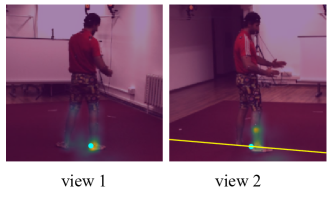
Figure 1: Comparison of epipolar line and attention module. Given the query pixel (cyan dot) in view 1 (current). The attention map on the view 2 (reference) indicates that the prediction relies on the image clues provided by the area of right shank, not just the corresponded right ankle. While previous methods based on epipolar line (yellow line) cannot capture this information.

2 Related Work

2.1 Multi-view 3D Pose Estimation

Multi-view 3D pose estimation usually follows a two-step process: (1) localize 2D joints with a 2D pose estimator on each view, and (2) lift the 2D joints from multi-view images to the 3D position via triangulation. To improve the performance of 2D pose detector, researchers typically resort to sophisticated architectures to capture both low-level and high-level representations [Wei et al.(2016)Wei, Ramakrishna, Kanade, and Sheikh, Chen et al.(2018b)Chen, Wang, Peng, Zhang, Yu, and Sun, Newell et al.(2016)Newell, Yang, and Deng, Xiao et al.(2018)Xiao, Wu, and Wei, Sun et al.(2019)Sun, Xiao, Liu, and Wang] or use the structural information to model the spatial constraints [Tompson et al.(2014)Tompson, Jain, LeCun, and Bregler, Kong et al.(2019)Kong, Chen, Ma, Yan, and Xie, Kong et al.(2020a)Kong, Ma, Chen, and Xie, Kong et al.(2020b)Kong, Ma, and Xie, Chen et al.(2020b)Chen, Ma, Kong, Yan, Wu, Fan, and Xie]. However, the occlusion cases are still challenging, as monocular images do not provide evidence for occlusion joints localization.

An alternative approach, more explainable, is to make the 2D pose detector 3D-aware, i.e., fusing the 2D feature heatmaps [Qiu et al.(2019)Qiu, Wang, Wang, Wang, and Zeng, Zhang et al.(2021)Zhang, Wang, Qiu, Qin, and Zeng, Xie et al.(2020)Xie, Wang, and Wang, Chen et al.(2021b)Chen, Lin, Xie, Lin, and Xie, He et al.(2020)He, Yan, Fragkiadaki, and Yu] from different views. Specifically, the Cross-view Fusion [Qiu et al.(2019)Qiu, Wang, Wang, Wang, and Zeng] directly learns a fixed attention weight to fuse all pairs of pixels given a pair of views. However, the learnable weight requires the multi-camera setup unchanged during the inference time, and the number of parameters is quadratic to the resolution of input images. The epipolar transformer [He et al.(2020)He, Yan, Fragkiadaki, and Yu] applies the non-local module [Wang et al.(2018)Wang, Girshick, Gupta, and He] to obtain the weights and only fuse pixels along the epipolar line in other views. Thus it is easy to learn and flexible to use. However, sampling along the epipolar line discards off-epipolar line information and thus obtains limited information from the reference views. In the second step, researchers use graphical model with the structure of human [Qiu et al.(2019)Qiu, Wang, Wang, Wang, and Zeng] to improve the quality of triangulation or directly learn 3D pose via differentiable triangulation [Iskakov et al.(2019)Iskakov, Burkov, Lempitsky, and Malkov]. Our work still focuses on enhancing 2D pose by fully integrating information from different views.

2.2 Transformer

Vision Transformer

Recently, several studies demonstrated that the transformer architectures [Vaswani et al.(2017)Vaswani, Shazeer, Parmar, Uszkoreit, Jones, Gomez, Kaiser, and Polosukhin] plays a significant role in a wide range of computer vision tasks, such as image classification [Dosovitskiy et al.(2020)Dosovitskiy, Beyer, Kolesnikov, Weissenborn, Zhai, Unterthiner, Dehghani, Minderer, Heigold, Gelly, et al., Touvron et al.(2020)Touvron, Cord, Douze, Massa, Sablayrolles, and Jégou, Chen et al.(2021a)Chen, Fan, and Panda], object detection [Carion et al.(2020)Carion, Massa, Synnaeve, Usunier, Kirillov, and Zagoruyko, Zhu et al.(2020)Zhu, Su, Lu, Li, Wang, and Dai], and semantic segmentation [Zheng et al.(2020)Zheng, Lu, Zhao, Zhu, Luo, Wang, Fu, Feng, Xiang, Torr, et al., Wang et al.(2020a)Wang, Xu, Wang, Shen, Cheng, Shen, and Xia, Yan et al.(2022)Yan, Tang, Sun, Ma, Kong, and Xie]. Recently, some studies also explored applying the transformer on human pose estimation tasks [Yang et al.(2020)Yang, Quan, Nie, and Yang, Li et al.(2021)Li, Wang, Zhang, Xu, Xu, and Tu, Mao et al.(2021)Mao, Ge, Shen, Tian, Wang, and Wang, Lin et al.(2020)Lin, Wang, and Liu, Zheng et al.(2021)Zheng, Zhu, Mendieta, Yang, Chen, and Ding]. More specifically, for 2D pose estimation, TransPose [Yang et al.(2020)Yang, Quan, Nie, and Yang] aims to explain the spatial dependencies of the predicted keypoints with transformers, PRTR [Li et al.(2021)Li, Wang, Zhang, Xu, Xu, and Tu] and TF-Pose [Mao et al.(2021)Mao, Ge, Shen, Tian, Wang, and Wang] attempt to directly regress the joint coordinates by transformer decoders. While for the 3D pose estimation, METRO [Lin et al.(2020)Lin, Wang, and Liu] firstly applies transformer to reconstruct 3D human pose and mesh from a single image, and PoseFormer [Zheng et al.(2021)Zheng, Zhu, Mendieta, Yang, Chen, and Ding] builds a spatial-temporal transformers with the input of 2D joint sequences for 3D pose estimation in videos. However, previous works have hardly exploited the transformer architectures on the multi-view 3D pose estimation setting, which is however an important task in the pose estimation area.

Multi-modal Transformer

Transformers with multi-modality inputs such as images and texts have also been fully exploited [Kim et al.(2021)Kim, Son, and Kim, Tan and Bansal(2019), Su et al.(2019)Su, Zhu, Cao, Li, Lu, Wei, and Dai, Li et al.(2020)Li, Duan, Fang, Gong, and Jiang, Zhuge et al.(2021)Zhuge, Gao, Fan, Jin, Chen, Zhou, Qiu, and Shao, You et al.(2021a)You, Chen, and Zou, You et al.(2021b)You, Chen, and Zou]. In general, these methods directly concatenate the embeddings from two sources together [Kim et al.(2021)Kim, Son, and Kim] and make the transformer itself to learn the correspondence between two modalities from millions of image-text paris [Sharma et al.(2018)Sharma, Ding, Goodman, and Soricut]. Thus, these methods are quite expensive and inefficient, and difficult to apply on limited datasets. Our method, however, directly provides the correspondence between two inputs and makes the transformer explicitly learn their relationships.

3 Methods

3.1 Overview

Figure 2 is an overview of TransFusion. It takes two images from different views as input, and predicts the heatmaps of joints in each view. The framework consists of three modules: a CNN backbone to extract low-level features; a transformer encoder to capture both correspondence between two views and long-range spatial correlations within single view images; a head to predict the heatmaps of joints. Specifically, given images $\mathbf{I}_{i}\in\mathbb{R}^{3\times H_{I}\times W_{I}}$ in each view, where $i\in\{1,2\}$ denotes view $1$ and view $2$, the backbone $\mathcal{F}(\cdot)$ firstly produces the low-level features $\mathbf{X}_{i}=\mathcal{F}(\mathbf{I}_{i})\in\mathbb{R}^{d\times H\times W}$ of each image. Here $d$ is the number of channels. $H$ and $W$ are the height and width of the feature map, respectively. The feature $\mathbf{X}_{i}$ is flattened into a sequence vector $\mathbf{X}_{i}^{{}^{\prime}}\in\mathbb{R}^{L\times d}$, where $L=H\times W$. Both 2D sine positional encoding $\mathbf{E_{2D}}$ and 3D geometry positional encoding $\mathbf{E_{G}}_{i}$ are added onto $\mathbf{X}_{i}^{{}^{\prime}}$ to make the transformer aware of position information. $\mathbf{X}_{1}^{{}^{\prime}}$ and $\mathbf{X}_{2}^{{}^{\prime}}$ are concatenated together to build a uniform embedding $\mathbf{X}=[\mathbf{X}_{1}^{{}^{\prime}}+\mathbf{E_{2D}}+\mathbf{E_{G}}_{1},\mathbf{X}_{2}^{{}^{\prime}}+\mathbf{E_{2D}}+\mathbf{E_{G}}_{2}]\in\mathbb{R}^{2L\times d}$. The embedding $\mathbf{X}$ then enters the standard transformer encoder $\mathcal{E}(\cdot)$. Finally, the output of the transformers $\mathbf{\tilde{X}}=\mathcal{E}(\mathbf{X})$ are split into $\tilde{\mathbf{X}_{1}}$ and $\tilde{\mathbf{X}_{2}}$, which is embedding of each view, and a prediction head $\mathcal{H}(\cdot)$ takes $\tilde{\mathbf{X}_{i}}$ and predicts the joint heatmaps $\bar{\mathbf{H}}_{i}=\mathcal{H}(\tilde{\mathbf{X}_{i}})\in\mathbb{R}^{k\times H_{h}\times W_{h}}$ for each view, where $k$ is the number of joints.

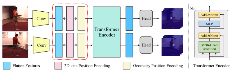
Figure 2: Overview of TransFusion.

3.2 TransFusion

Transformer Encoders

The transform encoder $\mathcal{E(\cdot)}$ consists of several layers of multi-head self-attention. Let $l=2L$ for short, given the input sequence $\mathbf{X}\in\mathbb{R}^{l\times d}$, the self-attention layer first uses linear projections to obtain a set of queries ($\mathbf{Q}\in\mathbb{R}^{l\times d}$), keys ($\mathbf{K}\in\mathbb{R}^{l\times d}$) and values ($\mathbf{V}\in\mathbb{R}^{l\times d}$) from $\mathbf{X}$. The three linear projections are parameterized by three learnable matrices $\mathbf{W}_{q}$, $\mathbf{W}_{k}$, $\mathbf{W}_{v}\in\mathbb{R}^{d\times d}$. Following [Carion et al.(2020)Carion, Massa, Synnaeve, Usunier, Kirillov, and Zagoruyko], the position encoding $\mathbf{E}$ is added into the input $\mathbf{X}$ for computing the query and key. The scaled dot-product attention [Vaswani et al.(2017)Vaswani, Shazeer, Parmar, Uszkoreit, Jones, Gomez, Kaiser, and Polosukhin] between $\mathbf{Q}$ and $\mathbf{K}$ is adopted to compute the attention weights, and aggregate the values:

$$\mathbf{A}=\operatorname{softmax}\left(\frac{\mathbf{QK}^{T}}{\sqrt{d}}\right)\mathbf{V}$$ (1)

Finally, a non-linear transformation (i.e., multi layer perceptron, and the skip connection) is applied on $\mathbf{A}$ to calculate the output $\tilde{\mathbf{X}}$. As $\mathbf{X}$ is low-level features of all views, given one query pixel on the feature map, it can attend cues from the its own view and other views simultaneously through the entire network.

Positional encoding

The attention layer would degenerate into a permutation-equivariant architecture without any position information. Thus, the positional encoding is necessary to make the transformer aware of position and order of input sequence. For each individual view, we follow the 2D sine positional encoding in the original transformers [Dosovitskiy et al.(2020)Dosovitskiy, Beyer, Kolesnikov, Weissenborn, Zhai, Unterthiner, Dehghani, Minderer, Heigold, Gelly, et al., Yang et al.(2020)Yang, Quan, Nie, and Yang], and we denote it as $\mathbf{E_{2D}}$. However, it only encodes position information from its own view, while the position information in the 3D space and that from the reference views cannot be encoded. Thus, another positional encoding $\mathbf{E_{G}}_{i}$ (See Section 3.3) is required to encode the 3D location information of each view $i$ in the 3D space.

3.3 Geometry Position Encoding (GPE)

To make the transformers 3D-aware, we introduce 3D camera information [Andrew(2001), Zhao et al.(2021)Zhao, Kong, and Fowlkes] into the positional encoding and propose the Geometry Positional Encoding. Denote the world coordinate system as $\mathbf{O}_{\text{world}}$. The 3D location of view $i$ ’s camera center in $\mathbf{O}_{\text{world}}$ is denoted as $\mathbf{C}_{i}$, and the 3D location of the $n$-th pixel ($n\in\{1,2,...,L\}$) of view $i$ in $\mathbf{O}_{\text{world}}$ is denoted as $\mathbf{P}_{i}^{n}$. $\mathbf{P}_{i}^{n}$ can be derived from the camera parameters of view $i$. As shown in Figure 3, the ray $\overrightarrow{\mathbf{C}_{i}\mathbf{P}_{i}^{n}}$ (gray line with arrow) indicates the direction of the pixel $p_{i}$ in the world. The unit vector $\widehat{\overrightarrow{\mathbf{C}_{i}\mathbf{P}_{i}^{n}}}$ is its direction vector, and can encode the relative 3D location of each pixel. Thus, we design GPE based on this unit vector, and we add one linear transformation to make it fit the input dimension $d$. The 3D geometry positional encoding for the $n$-th pixel in view $i$ is defined as:

$$\mathbf{E_{G}}_{i}^{n}=\mathbf{W}_{e}\widehat{\overrightarrow{\mathbf{C}_{i}\mathbf{P}_{i}^{n}}}\in\mathbb{R}^{d}$$ (2)

Where $\mathbf{W}_{e}\in\mathbb{R}^{d\times 3}$ is a learnable transformation matrix. With $\mathbf{E_{G}}_{i}$, the transformer can be aware of the 3D location of each view.

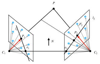
Figure 3: Illustration of Geometry Positional Encoding. For each pixel, its geometry positional encoding is calculated from the unit vector $\mathbf{\hat{u}_{i}^{n}}$ of ray ${\mathbf{C}_{i}\mathbf{P}_{i}}$ in the world coordinate $\mathbf{O}_{\text{world}}$.

3.4 Epipolar Field

Although GPE impose the 3D space information into transformers, it does not explicitly encode the relationship between two views. As a result, given a pixel in the current view, it is still difficult to attend the corresponding regions when performing global attention between features of two views. We further impose the Epipolar Constraints [Andrew(2001)] into GPE: Given one pixel $p_{1}$ in view $1$, its correspondence pixel $p_{2}$ in view $2$ must be on the epipolar line $l_{2}$ (Figure 3). However, the epipolar line does not model the relationship with pixels outside $l_{2}$. Instead, pixels close to the line and pixels away from the line should be treated differently. Thus, we propose the Epipolar Field to model the relationship among all pixels in the reference view. In detail, given $\mathbf{P}_{1}^{n}$, the 3D location of $n$-th pixel $p_{1}^{n}$ in view 1, we calculate the normal vector $\mathbf{N}_{\mathbf{P}_{1}^{n}\mathbf{C}_{1}\mathbf{C}_{2}}$ of plane $\mathbf{P}_{1}^{n}\mathbf{C}_{1}\mathbf{C}_{2}$ by:

$$\mathbf{N}_{\mathbf{P}_{1}^{n}\mathbf{C}_{1}\mathbf{C}_{2}}=\widehat{\overrightarrow{\mathbf{C}_{1}\mathbf{C}_{2}}}\times\widehat{\overrightarrow{\mathbf{C}_{1}\mathbf{P}_{1}^{n}}}$$ (3)

Given $\mathbf{P}_{2}^{m}$, the 3D location of $m$-th pixel $p_{2}^{m}$ in view $2$, we use the angle $\theta$ between the normal vector $\mathbf{N}_{\mathbf{P}_{1}^{n}\mathbf{C}_{1}\mathbf{C}_{2}}$ and ray $\overrightarrow{\mathbf{C}_{2}\mathbf{P}_{2}^{m}}$ to model the relationship between $p_{1}^{n}$ and $p_{2}^{m}$, and use the cosine of $\theta$ to calculate the correspondence score:

$$\mathbf{S}(p_{1}^{n},p_{2}^{m})=1-\mid\cos\theta\mid=1-\mid\mathbf{N}_{\mathbf{P}_{1}^{n}\mathbf{C}_{1}\mathbf{C}_{2}}\cdot\widehat{\overrightarrow{\mathbf{C}_{2}\mathbf{P}_{2}^{m}}}\mid$$ (4)

The absolute $\mid\cdot\mid$ is added to limit the score in $[0,1]$. With Eq. 4, if $p_{2}^{m}$ falls in the epipolar line $l_{2}$, the score $\mathbf{S}(p_{1}^{n},p_{2}^{m})$ will be $1$. Otherwise, the far $p_{2}^{m}$ is from $l_{2}$, the closer the score would be $0$. We further add a soft factor $\gamma$ to control the sharpness, thus the epipolar field is $\mathbf{S}^{\prime}(p_{1}^{n},p_{2}^{m})=(\mathbf{S}(p_{1}^{n},p_{2}^{m}))^{\gamma}$. Figure 4 gives a visualization of the epipolar field. Comparing with the epipolar line, the epipolar field model relationships with all pixels in the reference view. We can also reduce it to the epipolar line with a very large $\gamma$. Thus, epipolar field can be considered as a more general form of the epipolar line.

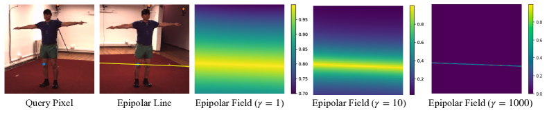
Figure 4: Illustration of Epipolar Field. The epipolar field can reflect the distance from the epipolar line to the off-line pixels. By adjusting the soft factor $\gamma$, it can also reduce to the standard epipolar line.

We then use the epipolar field to guide the learning of $\mathbf{W}_{e}$ to help the $\mathbf{E_{G}}_{i}^{n}$ encode correspondence between two views. In detail, we let the dot product of $\mathbf{E_{G}}_{1}^{n}$ and $\mathbf{E_{G}}_{2}^{m}$ match $\mathbf{S}^{\prime}(p_{1}^{n},p_{2}^{m})$ with the mean square error loss during the training process:

$$L_{\text{pos}}=\frac{1}{L^{2}}\sum_{n}^{L}\sum_{m}^{L}(\mathbf{E_{G}}_{1}^{n}{(\mathbf{E_{G}}_{2}^{m})}^{T}-\mathbf{S}^{\prime}(p_{1}^{n},p_{2}^{m}))^{2}$$ (5)

Therefore, a high attention score will be achieved along the epipolar line when calculating the cross-view attention maps between $\mathbf{X}_{1}^{{}^{\prime}}+\mathbf{E_{2D}}+\mathbf{E_{G}}_{1}$ and $\mathbf{X}_{2}^{{}^{\prime}}+\mathbf{E_{2D}}+\mathbf{E_{G}}_{2}$, which makes the transformer easy to attend corresponding regions. Moreover, with this soft design, semantic information from offline pixels are still kept, rather than discarded like [He et al.(2020)He, Yan, Fragkiadaki, and Yu].

3.5 Implementation Details

CNN backbone

We follow [Yang et al.(2020)Yang, Quan, Nie, and Yang] and apply a very shallow CNN architecture as the CNN backbone $\mathcal{F}(\cdot)$, which is the initial part of the ResNet-50 [He et al.(2016)He, Zhang, Ren, and Sun]. Specifically, the number of parameters of the shallow CNN is $1.4$ M, which is just $5.5\%$ of the original Simple Baseline with ResNet-50 ($25.6$M). The output feature map has size $H=H_{I}/8$, $W=W_{I}/8$. Thus, the fine-grained local feature information can still be kept.

TransFusion

Following [Carion et al.(2020)Carion, Massa, Synnaeve, Usunier, Kirillov, and Zagoruyko, Yang et al.(2020)Yang, Quan, Nie, and Yang], we set the dimension of the feature embedding $d$ to $256$, the number of heads to $8$, the number of encoder layers $N$ to $3$. Due to the limitation of resource, we only consider the fusion of $2$ neighborhood views, although out framework can be easily extended to more than $2$ views.

Prediction head

Given $\tilde{\mathbf{X}_{i}}$, we first reshape it back to $\tilde{\mathbf{X}_{i}^{{}^{\prime}}}\in\mathbb{R}^{d\times H\times W}$. The prediction head $\mathcal{H}(\cdot)$ applies one deconvolution layer and one $1\times 1$ convolution layer to predict the heatmap of keypoints. By default, the height and width of heatmaps $\mathbf{H}_{i}$ are $H_{h}=H_{I}/4$ and $W_{h}=W_{I}/4$.

Loss function

The groundtruth heatmap $\mathbf{H}_{i}\in\mathbb{R}^{k\times H_{h}\times W_{h}}$ of 2D keypoints is defined as a 2D a Gaussian centering around each keypoint [Wei et al.(2016)Wei, Ramakrishna, Kanade, and Sheikh]. We apply the Mean Square Error (MSE) loss to calculate the difference between the output heatmaps $\bar{\mathbf{H}}_{i}$ and $\mathbf{H}_{i}$. By combining the Equation 5, we train the network end-to-end with loss function $L=\frac{1}{HW}\parallel\bar{\mathbf{H}}_{i}-\mathbf{H}_{i}\parallel_{F}^{2}+L_{\text{pos}}$.

4 Experiments

4.1 Experimental Settings

Dataset

We conduct extensive experiments on two public multi-view 3D human pose estimation datasets, Human 3.6M [Ionescu et al.(2014)Ionescu, Papava, Olaru, and Sminchisescu, Catalin Ionescu(2011)] and Ski-Pose [Spörri(2016), Rhodin et al.(2018)Rhodin, Spörri, Katircioglu, Constantin, Meyer, Müller, Salzmann, and Fua, Gilgien et al.(2013)Gilgien, Spörri, Chardonnens, Kröll, and Müller, Gilgien et al.(2014)Gilgien, Spörri, Limpach, Geiger, and Müller, Gilgien et al.(2015)Gilgien, Spörri, Chardonnens, Kröll, Limpach, and Müller, Fasel et al.(2016)Fasel, Spörri, Gilgien, Boffi, Chardonnens, Müller, and Aminian, Fasel et al.(2017)Fasel, Spörri, Chardonnens, Kröll, Müller, and Aminian]. (1) The Human 3.6M contains joint annotations of video frames captured by four calibrated cameras in a room. We adopt the same training and test split as in [Qiu et al.(2019)Qiu, Wang, Wang, Wang, and Zeng, Iskakov et al.(2019)Iskakov, Burkov, Lempitsky, and Malkov, He et al.(2020)He, Yan, Fragkiadaki, and Yu], where subjects 1, 5, 6, 7, 8 are used for training, and 9, 11 are for testing. Note that 3D annotations of some scenes of the ’S9’ are damaged [Iskakov et al.(2019)Iskakov, Burkov, Lempitsky, and Malkov], we exclude these scenes from the evaluation as in [Iskakov et al.(2019)Iskakov, Burkov, Lempitsky, and Malkov, He et al.(2020)He, Yan, Fragkiadaki, and Yu]. (2) The Ski-Pose dataset aims to help analyze skiers’s giant slalom runs with 6 calibrated cameras. It provides six camera views as well as corresponding 3D pose. In detail, 8,481 frames are used for training and $1,716$ are used for testing. We resize all images to $256\times 256$ in all experiments.

Training

As the training of transformers requires huge datasets [Vaswani et al.(2017)Vaswani, Shazeer, Parmar, Uszkoreit, Jones, Gomez, Kaiser, and Polosukhin, Dosovitskiy et al.(2020)Dosovitskiy, Beyer, Kolesnikov, Weissenborn, Zhai, Unterthiner, Dehghani, Minderer, Heigold, Gelly, et al.], while the scenes of multi-view pose datasets are quite limited, making it difficult to train the transformer from scratch. By convention [Iskakov et al.(2019)Iskakov, Burkov, Lempitsky, and Malkov, He et al.(2020)He, Yan, Fragkiadaki, and Yu], we use the MS-COCO [Lin et al.(2014)Lin, Maire, Belongie, Hays, Perona, Ramanan, Dollár, and Zitnick] pretrained TransPose [Yang et al.(2020)Yang, Quan, Nie, and Yang] to initialize our network and fine tune it on the multi-view human pose datasets. Following the settings in [He et al.(2020)He, Yan, Fragkiadaki, and Yu], we apply Adam optimizer [Kingma and Ba(2014)] and train the model for $20$ epochs. The learning rate is initialized with $0.001$ and decays at $10$-th and $15$-th epoch with ratio $0.1$.

Evaluation metrics

The performance of 2D pose estimation is evaluated by Joint Detection Rate (JDR), which measures the percentage of the successfully detected keypoints. A keypoints is detected if the distance between the predicted location and the ground truth is within a predefined threshold. The threshold is set to half of the head size for human pose estimation. Given the estimated 2D joints of each view, following [Qiu et al.(2019)Qiu, Wang, Wang, Wang, and Zeng, He et al.(2020)He, Yan, Fragkiadaki, and Yu], direct triangulation is used for estimating the 3D poses with respect to the global coordinates. The 3D pose estimation accuracy is measured by Mean Per Joint Position Error (MPJPE) between the groundtruth 3D pose and the estimated 3D pose.

4.2 Results on Human 3.6M

We compare with two state-of-the-art methods, the crossview fusion [Qiu et al.(2019)Qiu, Wang, Wang, Wang, and Zeng] and the epipolar transformers [He et al.(2020)He, Yan, Fragkiadaki, and Yu]. For fair comparison, we use the SimpleBaseline-ResNet50 pretrained on COCO [Xiao et al.(2018)Xiao, Wu, and Wei] as initialization and then finetuned with their official codes [Qiu et al.(2019)Qiu, Wang, Wang, Wang, and Zeng, He et al.(2020)He, Yan, Fragkiadaki, and Yu].

Quantitative results

The results of both 2D and 3D pose estimation are shown in Table 1. We also shown the number of parameters of each model, the MACs (multiply-add operations). Besides, we also report the inference time to obtain the 3D pose from 4 views on a single 2080Ti GPU of all multiview methods. For both 2D and 3D pose estimation, TransFusion consistently outperforms or achieves comparable performance with epipolar transformers [He et al.(2020)He, Yan, Fragkiadaki, and Yu] and cross-view fusion [Qiu et al.(2019)Qiu, Wang, Wang, Wang, and Zeng]. Note that JDR is a relative loose metric, with a wider threshold which tolerates small errors, so the improvement on 2D is not very obvious. However, on the 3D metric, which directly computes the distance, our improvement is much more significant. Moreover, as in Table 2, our method can achieve significant improvement on sophisticated poses sequences such as "Phone" and "Smoke", which usually encounters heave occlusions for certain views. This result suggests that fusing features from the entire images of other views, instead of just features along the epipolar line [He et al.(2020)He, Yan, Fragkiadaki, and Yu], can bring more benefits. Besides, comparing to the single view TransPose [Yang et al.(2020)Yang, Quan, Nie, and Yang], our Transfusion can achieve $4.7$ mm gain on 3D. Thus, the improvement is not only from the TransPose architecture, but from the fusion with other views. Moreover, our method is lightweight and efficient. It only requires $2.1\%$ (5M / 235M) of the parameters of cross-view fusion [Qiu et al.(2019)Qiu, Wang, Wang, Wang, and Zeng]. Benefit from the parallel computing of transformers architectures, it further reduces the inference time, while the operation of sampling along epipolar lines [He et al.(2020)He, Yan, Fragkiadaki, and Yu] is time-consuming.

Method	Params	MACs	Inference Time (s)	JDR (%) $\uparrow$	MPJPE (mm) $\downarrow$
Single view - Simple Baseline[Xiao et al.(2018)Xiao, Wu, and Wei]	34M	51.7G	-	98.5	30.2
Single view - TransPose [Yang et al.(2020)Yang, Quan, Nie, and Yang]	5M	43.6G	-	98.6	30.5
Crossview Fusion [Qiu et al.(2019)Qiu, Wang, Wang, Wang, and Zeng]	235M	55.1G	0.048	99.4	27.8
Epipolar Transformer [He et al.(2020)He, Yan, Fragkiadaki, and Yu]	34M	51.7G	0.086	98.6	27.1
TransFusion	5M	50.2G	0.032	99.4	25.8

Table 1: 2D and 3D pose estimation accuracy comparison on Human3.6M. The metric of 2D pose is JDR (%), and the metric of 3D pose is MPJPE (mm). All networks are pretrained on COCO [Lin et al.(2014)Lin, Maire, Belongie, Hays, Perona, Ramanan, Dollár, and Zitnick] and then finetuned on Human 3.6M [Ionescu et al.(2014)Ionescu, Papava, Olaru, and Sminchisescu]. All images are resized to $256\times 256$.

Method	Dir	Disc	Eat	Greet	Phone	Pose	Purch	Sit	SitD	Smoke	Photo	Wait	WalkD	Walk	WalkT
Crossview Fusion[Qiu et al.(2019)Qiu, Wang, Wang, Wang, and Zeng]	24.0	28.8	25.6	24.5	28.3	24.4	26.9	30.7	34.4	29.0	32.6	25.1	24.3	30.8	24.9
Epipolar transformers [He et al.(2020)He, Yan, Fragkiadaki, and Yu]	23.2	27.1	23.4	22.4	32.4	21.4	22.6	37.3	35.4	29.0	27.7	24.2	21.2	26.6	22.3
TransFusion	24.4	26.4	23.4	21.1	25.2	23.2	24.7	33.8	29.8	26.4	26.8	24.2	23.2	26.1	23.3

Table 2: The MPJPE of each pose sequence on Human 3.6M.

Visualization of Attention maps

Given the query pixel in one view, we further visualize the attention maps on both views. We show our results in Figure 5. It is observed that on the view itself, typically the attention map is around the joints. If the query joint is occluded, it may resort to joints on the other side of the symmetry [Yang et al.(2020)Yang, Quan, Nie, and Yang]. On the neighboring view, the network usually not just attends the corresponding keypoint, but attends the whole limbs, which cannot be located by the epipolar line. Previous methods based on epipoar line [He et al.(2020)He, Yan, Fragkiadaki, and Yu] actually miss this important clue.

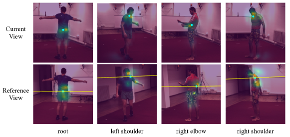
Figure 5: Visualization of attention maps on Human 3.6M test set. The cyan dots are groundtruth. Given the query pixel, the first rows are attention maps of current views, and the second rows are attention maps of reference views. We also visualize the epipolar line (yellow) for comparison.

Qualitative results

We also present examples of predicted 2D keypoints on the image and 3D pose in the space, and compare our methods with baseline methods [Qiu et al.(2019)Qiu, Wang, Wang, Wang, and Zeng]. As in Figure 6, even if the entire arms (green line) are occluded, our method still predicts the 2D keypoints correctly by fusing information from the reference view, and further gives a better 3D pose.

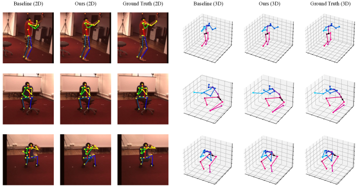
Figure 6: Visualization of predictions for Human 3.6M. Both skeletons of 2D keypoints on the image and 3D pose in the space are presented.

4.3 Ablation Studies

Geometry Positional Encoding

We conduct ablation studies on the GPE to verify its significance. In detail, we consider 3 settings: 1) training without 3D geometry positional encoding, 2) applying a learnable 3D positional encoding, i.e., directly learn $\mathbf{E_{G}}_{i}$ from scratch 3) training the 3D GPE without epipolar field constraints $L_{\text{pos}}$. Table 3 presents the results. Without the 3D location information, the performance of 1) and 2) are even worse than the single view TransPose, we hypothesize that the 2D sine PE makes the transformer easy to attend the same pixel location of all views, and the learned 3D PE is easy to overfit the training examples. Without $L_{\text{pos}}$, the error will also increase. Thus the guide from the epipolar field is favorable, as it imposes correspondence for cross-view attention.

Method	2D Pose / JDR (%) $\uparrow$	3D Pose / MPJPE (mm) $\downarrow$
TransFusion - without 3D positional encoding	98.5	35.9
TransFusion - learnable 3D positional encoding	96.0	57.3
TransFusion - GPE without $L_{\text{pos}}$	99.3	26.8
TransFusion	99.4	25.8

Table 3: Ablation studies on different types of 3D positional encoding

Soft Factor $\gamma$

We also try different values of the soft vector $\gamma$, results are shown in Figure 7(a). With a small $\gamma$, the epipolar field assign all locations with relative high probabilities, the performance are slightly worse (1.3 mm drop). While with a huge $\gamma=1000$, the epipolar field reduces to the hard epipolar line, and the performance drops $2.7$ mm. Thus, we verify the effectiveness of our epipolar field compared with hard-coded epipolar line.

Transformer architecture

We study how performance scales with the size of the transformer. As in Figure 7(b), with the number of layers $N$ increasing, the performance improves significantly, as the learning ability of transformer is more powerful with more parameters. But when $N>3$, it tends to saturate or degenerate. We hypothesize that the transformer is easy to overfit when the size is too huge. Meanwhile, as in Figure 7(c), with the number of heads increases, the performance also improves gradually, as more heads can help attend different features [Vaswani et al.(2017)Vaswani, Shazeer, Parmar, Uszkoreit, Jones, Gomez, Kaiser, and Polosukhin]. In summary, our choice with $N=3$ and 8 heas are reasonable.

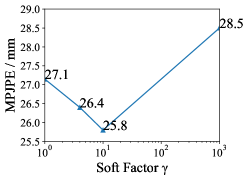
(a) Soft Factor

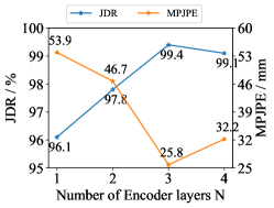
(b) Number of encoder layers

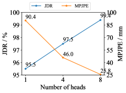
(c) Number of heads

Figure 7: Ablation studies on the soft factor $\gamma$ of the epipolar field, the number of transformer encoder layers $N$, and the number of transformer heads.

Method	2D Pose / JDR (%) $\uparrow$	3D Pose / MPJPE (mm) $\downarrow$
Single view - Simple Baseline [Xiao et al.(2018)Xiao, Wu, and Wei]	94.5	39.6
Epipolar Transformer [He et al.(2020)He, Yan, Fragkiadaki, and Yu]	94.9	34.2
TransFusion	96.0	31.6

Table 4: 2D and 3D pose estimation accuracy comparison on Ski-Pose.

4.4 Results on Ski-Pose Dataset

We further apply TransFusion on the Ski-Pose dataset to verify its generalization ability. Results are presented in Table 4. In the settings with six cameras, the Crossview Fusion is too huge (537M) to train on the 2080Ti GPU. Similar to Human 3.6M, TransFusion still outperform or achieve comparable performance with other fusion methods, while it is much lightweight. Thus, our method is also effective in outdoor multi-view settings.

5 Conclusion

In this paper, we apply the transformer to the multi-view 3D human pose estimation for the first time. Inspired by multi-modal transformers, we propose the TransFusion network, a lightweight architecture to integrate cues from both self views and reference views. Furthermore, we propose the epipolar field, and apply it to the 3D positional encoding to encode correspondence between two views explicitly. Experimental results shows that our method outperform previous fusion methods but with a more light weighted network. In the future we plan to apply our TransFusion to regress the 3D locations with multi-view inputs in an end-to-end way to further improve 3D predictions.

References

- [Andrew(2001)] Alex M Andrew. Multiple view geometry in computer vision. Kybernetes, 2001.
- [Carion et al.(2020)Carion, Massa, Synnaeve, Usunier, Kirillov, and Zagoruyko] Nicolas Carion, Francisco Massa, Gabriel Synnaeve, Nicolas Usunier, Alexander Kirillov, and Sergey Zagoruyko. End-to-end object detection with transformers. In European Conference on Computer Vision, pages 213–229. Springer, 2020.
- [Catalin Ionescu(2011)] Cristian Sminchisescu Catalin Ionescu, Fuxin Li. Latent structured models for human pose estimation. In International Conference on Computer Vision, 2011.
- [Chen et al.(2021a)Chen, Fan, and Panda] Chun-Fu Chen, Quanfu Fan, and Rameswar Panda. Crossvit: Cross-attention multi-scale vision transformer for image classification. arXiv preprint arXiv:2103.14899, 2021a.
- [Chen et al.(2018a)Chen, Lin, Xie, Tang, Xue, Xie, Lin, and Fan] Liangjian Chen, Shih-Yao Lin, Yusheng Xie, Hui Tang, Yufan Xue, Xiaohui Xie, Yen-Yu Lin, and Wei Fan. Generating realistic training images based on tonality-alignment generative adversarial networks for hand pose estimation. arXiv preprint arXiv:1811.09916, 2018a.
- [Chen et al.(2020a)Chen, Lin, Xie, Lin, Fan, and Xie] Liangjian Chen, Shih-Yao Lin, Yusheng Xie, Yen-Yu Lin, Wei Fan, and Xiaohui Xie. Dggan: Depth-image guided generative adversarial networks for disentangling rgb and depth images in 3d hand pose estimation. In Proceedings of the IEEE/CVF Winter Conference on Applications of Computer Vision, pages 411–419, 2020a.
- [Chen et al.(2021b)Chen, Lin, Xie, Lin, and Xie] Liangjian Chen, Shih-Yao Lin, Yusheng Xie, Yen-Yu Lin, and Xiaohui Xie. Mvhm: A large-scale multi-view hand mesh benchmark for accurate 3d hand pose estimation. In Proceedings of the IEEE/CVF Winter Conference on Applications of Computer Vision, pages 836–845, 2021b.
- [Chen et al.(2020b)Chen, Ma, Kong, Yan, Wu, Fan, and Xie] Yifei Chen, Haoyu Ma, Deying Kong, Xiangyi Yan, Jianbao Wu, Wei Fan, and Xiaohui Xie. Nonparametric structure regularization machine for 2d hand pose estimation. In Proceedings of the IEEE/CVF Winter Conference on Applications of Computer Vision, pages 381–390, 2020b.
- [Chen et al.(2021c)Chen, Ma, Wang, Wu, Wu, and Xie] Yifei Chen, Haoyu Ma, Jiangyuan Wang, Jianbao Wu, Xian Wu, and Xiaohui Xie. Pd-net: Quantitative motor function evaluation for parkinson’s disease via automated hand gesture analysis. In Proceedings of the 27th ACM SIGKDD Conference on Knowledge Discovery & Data Mining, pages 2683–2691, 2021c.
- [Chen et al.(2018b)Chen, Wang, Peng, Zhang, Yu, and Sun] Yilun Chen, Zhicheng Wang, Yuxiang Peng, Zhiqiang Zhang, Gang Yu, and Jian Sun. Cascaded pyramid network for multi-person pose estimation. In Proceedings of the IEEE conference on computer vision and pattern recognition, pages 7103–7112, 2018b.
- [Dosovitskiy et al.(2020)Dosovitskiy, Beyer, Kolesnikov, Weissenborn, Zhai, Unterthiner, Dehghani, Minderer, Heigold, Gelly, et al.] Alexey Dosovitskiy, Lucas Beyer, Alexander Kolesnikov, Dirk Weissenborn, Xiaohua Zhai, Thomas Unterthiner, Mostafa Dehghani, Matthias Minderer, Georg Heigold, Sylvain Gelly, et al. An image is worth 16x16 words: Transformers for image recognition at scale. arXiv preprint arXiv:2010.11929, 2020.
- [Fasel et al.(2016)Fasel, Spörri, Gilgien, Boffi, Chardonnens, Müller, and Aminian] Benedikt Fasel, Jörg Spörri, Matthias Gilgien, Geo Boffi, Julien Chardonnens, Erich Müller, and Kamiar Aminian. Three-dimensional body and centre of mass kinematics in alpine ski racing using differential gnss and inertial sensors. Remote Sensing, 8(8):671, 2016.
- [Fasel et al.(2017)Fasel, Spörri, Chardonnens, Kröll, Müller, and Aminian] Benedikt Fasel, Jörg Spörri, Julien Chardonnens, Josef Kröll, Erich Müller, and Kamiar Aminian. Joint inertial sensor orientation drift reduction for highly dynamic movements. IEEE journal of biomedical and health informatics, 22(1):77–86, 2017.
- [Ge et al.(2019)Ge, Ren, Li, Xue, Wang, Cai, and Yuan] Liuhao Ge, Zhou Ren, Yuncheng Li, Zehao Xue, Yingying Wang, Jianfei Cai, and Junsong Yuan. 3d hand shape and pose estimation from a single rgb image. In Proceedings of the IEEE Conference on Computer Vision and Pattern Recognition, pages 10833–10842, 2019.
- [Gilgien et al.(2013)Gilgien, Spörri, Chardonnens, Kröll, and Müller] Matthias Gilgien, Jörg Spörri, Julien Chardonnens, Josef Kröll, and Erich Müller. Determination of external forces in alpine skiing using a differential global navigation satellite system. Sensors, 13(8):9821–9835, 2013.
- [Gilgien et al.(2014)Gilgien, Spörri, Limpach, Geiger, and Müller] Matthias Gilgien, Jörg Spörri, Philippe Limpach, Alain Geiger, and Erich Müller. The effect of different global navigation satellite system methods on positioning accuracy in elite alpine skiing. Sensors, 14(10):18433–18453, 2014.
- [Gilgien et al.(2015)Gilgien, Spörri, Chardonnens, Kröll, Limpach, and Müller] Matthias Gilgien, Jörg Spörri, Julien Chardonnens, Josef Kröll, Philippe Limpach, and Erich Müller. Determination of the centre of mass kinematics in alpine skiing using differential global navigation satellite systems. Journal of sports sciences, 33(9):960–969, 2015.
- [He et al.(2016)He, Zhang, Ren, and Sun] Kaiming He, Xiangyu Zhang, Shaoqing Ren, and Jian Sun. Deep residual learning for image recognition. In Proceedings of the IEEE conference on computer vision and pattern recognition, pages 770–778, 2016.
- [He et al.(2020)He, Yan, Fragkiadaki, and Yu] Yihui He, Rui Yan, Katerina Fragkiadaki, and Shoou-I Yu. Epipolar transformers. In Proceedings of the IEEE/CVF Conference on Computer Vision and Pattern Recognition, pages 7779–7788, 2020.
- [Ionescu et al.(2014)Ionescu, Papava, Olaru, and Sminchisescu] Catalin Ionescu, Dragos Papava, Vlad Olaru, and Cristian Sminchisescu. Human3.6m: Large scale datasets and predictive methods for 3d human sensing in natural environments. IEEE Transactions on Pattern Analysis and Machine Intelligence, 36(7):1325–1339, jul 2014.
- [Iskakov et al.(2019)Iskakov, Burkov, Lempitsky, and Malkov] Karim Iskakov, Egor Burkov, Victor Lempitsky, and Yury Malkov. Learnable triangulation of human pose. In Proceedings of the IEEE/CVF International Conference on Computer Vision, pages 7718–7727, 2019.
- [Kim et al.(2021)Kim, Son, and Kim] Wonjae Kim, Bokyung Son, and Ildoo Kim. Vilt: Vision-and-language transformer without convolution or region supervision. arXiv preprint arXiv:2102.03334, 2021.
- [Kingma and Ba(2014)] Diederik P Kingma and Jimmy Ba. Adam: A method for stochastic optimization. arXiv preprint arXiv:1412.6980, 2014.
- [Kong et al.(2019)Kong, Chen, Ma, Yan, and Xie] Deying Kong, Yifei Chen, Haoyu Ma, Xiangyi Yan, and Xiaohui Xie. Adaptive graphical model network for 2d handpose estimation. arXiv preprint arXiv:1909.08205, 2019.
- [Kong et al.(2020a)Kong, Ma, Chen, and Xie] Deying Kong, Haoyu Ma, Yifei Chen, and Xiaohui Xie. Rotation-invariant mixed graphical model network for 2d hand pose estimation. In Proceedings of the IEEE/CVF Winter Conference on Applications of Computer Vision, pages 1546–1555, 2020a.
- [Kong et al.(2020b)Kong, Ma, and Xie] Deying Kong, Haoyu Ma, and Xiaohui Xie. Sia-gcn: A spatial information aware graph neural network with 2d convolutions for hand pose estimation. arXiv preprint arXiv:2009.12473, 2020b.
- [Li et al.(2020)Li, Duan, Fang, Gong, and Jiang] Gen Li, Nan Duan, Yuejian Fang, Ming Gong, and Daxin Jiang. Unicoder-vl: A universal encoder for vision and language by cross-modal pre-training. In Proceedings of the AAAI Conference on Artificial Intelligence, pages 11336–11344, 2020.
- [Li et al.(2021)Li, Wang, Zhang, Xu, Xu, and Tu] Ke Li, Shijie Wang, Xiang Zhang, Yifan Xu, Weijian Xu, and Zhuowen Tu. Pose recognition with cascade transformers. arXiv preprint arXiv:2104.06976, 2021.
- [Lin et al.(2020)Lin, Wang, and Liu] Kevin Lin, Lijuan Wang, and Zicheng Liu. End-to-end human pose and mesh reconstruction with transformers. arXiv preprint arXiv:2012.09760, 2020.
- [Lin et al.(2014)Lin, Maire, Belongie, Hays, Perona, Ramanan, Dollár, and Zitnick] Tsung-Yi Lin, Michael Maire, Serge Belongie, James Hays, Pietro Perona, Deva Ramanan, Piotr Dollár, and C Lawrence Zitnick. Microsoft coco: Common objects in context. In European conference on computer vision, pages 740–755. Springer, 2014.
- [Mao et al.(2021)Mao, Ge, Shen, Tian, Wang, and Wang] Weian Mao, Yongtao Ge, Chunhua Shen, Zhi Tian, Xinlong Wang, and Zhibin Wang. Tfpose: Direct human pose estimation with transformers. arXiv preprint arXiv:2103.15320, 2021.
- [Mehta et al.(2017)Mehta, Sridhar, Sotnychenko, Rhodin, Shafiei, Seidel, Xu, Casas, and Theobalt] Dushyant Mehta, Srinath Sridhar, Oleksandr Sotnychenko, Helge Rhodin, Mohammad Shafiei, Hans-Peter Seidel, Weipeng Xu, Dan Casas, and Christian Theobalt. Vnect: Real-time 3d human pose estimation with a single rgb camera. ACM Transactions on Graphics (TOG), 36(4):1–14, 2017.
- [Newell et al.(2016)Newell, Yang, and Deng] Alejandro Newell, Kaiyu Yang, and Jia Deng. Stacked hourglass networks for human pose estimation. In European conference on computer vision, pages 483–499. Springer, 2016.
- [Qiu et al.(2019)Qiu, Wang, Wang, Wang, and Zeng] Haibo Qiu, Chunyu Wang, Jingdong Wang, Naiyan Wang, and Wenjun Zeng. Cross view fusion for 3d human pose estimation. In Proceedings of the IEEE/CVF International Conference on Computer Vision, pages 4342–4351, 2019.
- [Rhodin et al.(2018)Rhodin, Spörri, Katircioglu, Constantin, Meyer, Müller, Salzmann, and Fua] Helge Rhodin, Jörg Spörri, Isinsu Katircioglu, Victor Constantin, Frédéric Meyer, Erich Müller, Mathieu Salzmann, and Pascal Fua. Learning monocular 3d human pose estimation from multi-view images. In Proceedings of the IEEE Conference on Computer Vision and Pattern Recognition, pages 8437–8446, 2018.
- [Sharma et al.(2018)Sharma, Ding, Goodman, and Soricut] Piyush Sharma, Nan Ding, Sebastian Goodman, and Radu Soricut. Conceptual captions: A cleaned, hypernymed, image alt-text dataset for automatic image captioning. In Proceedings of the 56th Annual Meeting of the Association for Computational Linguistics (Volume 1: Long Papers), pages 2556–2565, 2018.
- [Simon et al.(2017)Simon, Joo, Matthews, and Sheikh] Tomas Simon, Hanbyul Joo, Iain Matthews, and Yaser Sheikh. Hand keypoint detection in single images using multiview bootstrapping. In Proceedings of the IEEE conference on Computer Vision and Pattern Recognition, pages 1145–1153, 2017.
- [Spörri(2016)] Jörg Spörri. Reasearch dedicated to sports injury prevention-the’sequence of prevention’on the example of alpine ski racing. Habilitation with Venia Docendi in Biomechanics, 1(2):7, 2016.
- [Su et al.(2019)Su, Zhu, Cao, Li, Lu, Wei, and Dai] Weijie Su, Xizhou Zhu, Yue Cao, Bin Li, Lewei Lu, Furu Wei, and Jifeng Dai. Vl-bert: Pre-training of generic visual-linguistic representations. arXiv preprint arXiv:1908.08530, 2019.
- [Sun et al.(2019)Sun, Xiao, Liu, and Wang] Ke Sun, Bin Xiao, Dong Liu, and Jingdong Wang. Deep high-resolution representation learning for human pose estimation. In Proceedings of the IEEE Conference on Computer Vision and Pattern Recognition, pages 5693–5703, 2019.
- [Tan and Bansal(2019)] Hao Tan and Mohit Bansal. Lxmert: Learning cross-modality encoder representations from transformers. arXiv preprint arXiv:1908.07490, 2019.
- [Tang et al.(2021)Tang, Liu, Han, Xie, Chen, Qian, Liu, Sun, and Bai] Hao Tang, Xingwei Liu, Kun Han, Xiaohui Xie, Xuming Chen, Huang Qian, Yong Liu, Shanlin Sun, and Narisu Bai. Spatial context-aware self-attention model for multi-organ segmentation. In Proceedings of the IEEE/CVF Winter Conference on Applications of Computer Vision, pages 939–949, 2021.
- [Tome et al.(2017)Tome, Russell, and Agapito] Denis Tome, Chris Russell, and Lourdes Agapito. Lifting from the deep: Convolutional 3d pose estimation from a single image. In Proceedings of the IEEE Conference on Computer Vision and Pattern Recognition, pages 2500–2509, 2017.
- [Tompson et al.(2014)Tompson, Jain, LeCun, and Bregler] Jonathan J Tompson, Arjun Jain, Yann LeCun, and Christoph Bregler. Joint training of a convolutional network and a graphical model for human pose estimation. Advances in neural information processing systems, 27:1799–1807, 2014.
- [Touvron et al.(2020)Touvron, Cord, Douze, Massa, Sablayrolles, and Jégou] Hugo Touvron, Matthieu Cord, Matthijs Douze, Francisco Massa, Alexandre Sablayrolles, and Hervé Jégou. Training data-efficient image transformers & distillation through attention. arXiv preprint arXiv:2012.12877, 2020.
- [Vaswani et al.(2017)Vaswani, Shazeer, Parmar, Uszkoreit, Jones, Gomez, Kaiser, and Polosukhin] Ashish Vaswani, Noam Shazeer, Niki Parmar, Jakob Uszkoreit, Llion Jones, Aidan N Gomez, Lukasz Kaiser, and Illia Polosukhin. Attention is all you need. arXiv preprint arXiv:1706.03762, 2017.
- [Wang et al.(2018)Wang, Girshick, Gupta, and He] Xiaolong Wang, Ross Girshick, Abhinav Gupta, and Kaiming He. Non-local neural networks. In Proceedings of the IEEE conference on computer vision and pattern recognition, pages 7794–7803, 2018.
- [Wang et al.(2020a)Wang, Xu, Wang, Shen, Cheng, Shen, and Xia] Yuqing Wang, Zhaoliang Xu, Xinlong Wang, Chunhua Shen, Baoshan Cheng, Hao Shen, and Huaxia Xia. End-to-end video instance segmentation with transformers. arXiv preprint arXiv:2011.14503, 2020a.
- [Wang et al.(2019)Wang, Chen, Rathore, Shin, and Fowlkes] Zhe Wang, Liyan Chen, Shaurya Rathore, Daeyun Shin, and Charless Fowlkes. Geometric pose affordance: 3d human pose with scene constraints. arXiv preprint arXiv:1905.07718, 2019.
- [Wang et al.(2020b)Wang, Shin, and Fowlkes] Zhe Wang, Daeyun Shin, and Charless C Fowlkes. Predicting camera viewpoint improves cross-dataset generalization for 3d human pose estimation. In European Conference on Computer Vision, pages 523–540. Springer, 2020b.
- [Wang et al.(2022)Wang, Chen, Li, Liu, Xiong, Tighe, and Fowlkes] Zhe Wang, Hao Chen, Xinyu Li, Chunhui Liu, Yuanjun Xiong, Joseph Tighe, and Charless C Fowlkes. Sscap: Self-supervised co-occurrence action parsing for unsupervised temporal action segmentation. In Proceedings of the IEEE/CVF Winter Conference on Applications of Computer Vision, 2022.
- [Wei et al.(2016)Wei, Ramakrishna, Kanade, and Sheikh] Shih-En Wei, Varun Ramakrishna, Takeo Kanade, and Yaser Sheikh. Convolutional pose machines. In Proceedings of the IEEE conference on Computer Vision and Pattern Recognition, pages 4724–4732, 2016.
- [Xiao et al.(2018)Xiao, Wu, and Wei] Bin Xiao, Haiping Wu, and Yichen Wei. Simple baselines for human pose estimation and tracking. In Proceedings of the European conference on computer vision (ECCV), pages 466–481, 2018.
- [Xie et al.(2020)Xie, Wang, and Wang] Rongchang Xie, Chunyu Wang, and Yizhou Wang. Metafuse: A pre-trained fusion model for human pose estimation. In Proceedings of the IEEE/CVF Conference on Computer Vision and Pattern Recognition, pages 13686–13695, 2020.
- [Yan et al.(2022)Yan, Tang, Sun, Ma, Kong, and Xie] Xiangyi Yan, Hao Tang, Shanlin Sun, Haoyu Ma, Deying Kong, and Xiaohui Xie. After-unet: Axial fusion transformer unet for medical image segmentation. In Proceedings of the IEEE/CVF Winter Conference on Applications of Computer Vision, 2022.
- [Yang et al.(2020)Yang, Quan, Nie, and Yang] Sen Yang, Zhibin Quan, Mu Nie, and Wankou Yang. Transpose: Towards explainable human pose estimation by transformer. arXiv preprint arXiv:2012.14214, 2020.
- [You et al.(2021a)You, Chen, and Zou] Chenyu You, Nuo Chen, and Yuexian Zou. MRD-Net: Multi-Modal Residual Knowledge Distillation for Spoken Question Answering. In IJCAI, 2021a.
- [You et al.(2021b)You, Chen, and Zou] Chenyu You, Nuo Chen, and Yuexian Zou. Self-supervised contrastive cross-modality representation learning for spoken question answering. arXiv preprint arXiv:2109.03381, 2021b.
- [Zhang et al.(2019)Zhang, Li, Mo, Zhang, and Zheng] Xiong Zhang, Qiang Li, Hong Mo, Wenbo Zhang, and Wen Zheng. End-to-end hand mesh recovery from a monocular rgb image. In Proceedings of the IEEE International Conference on Computer Vision, pages 2354–2364, 2019.
- [Zhang et al.(2021)Zhang, Wang, Qiu, Qin, and Zeng] Zhe Zhang, Chunyu Wang, Weichao Qiu, Wenhu Qin, and Wenjun Zeng. Adafuse: Adaptive multiview fusion for accurate human pose estimation in the wild. International Journal of Computer Vision, 129(3):703–718, 2021.
- [Zhao et al.(2021)Zhao, Kong, and Fowlkes] Yunhan Zhao, Shu Kong, and Charless Fowlkes. Camera pose matters: Improving depth prediction by mitigating pose distribution bias. In Proceedings of the IEEE/CVF Conference on Computer Vision and Pattern Recognition, pages 15759–15768, 2021.
- [Zheng et al.(2021)Zheng, Zhu, Mendieta, Yang, Chen, and Ding] Ce Zheng, Sijie Zhu, Matias Mendieta, Taojiannan Yang, Chen Chen, and Zhengming Ding. 3d human pose estimation with spatial and temporal transformers. arXiv preprint arXiv:2103.10455, 2021.
- [Zheng et al.(2020)Zheng, Lu, Zhao, Zhu, Luo, Wang, Fu, Feng, Xiang, Torr, et al.] Sixiao Zheng, Jiachen Lu, Hengshuang Zhao, Xiatian Zhu, Zekun Luo, Yabiao Wang, Yanwei Fu, Jianfeng Feng, Tao Xiang, Philip HS Torr, et al. Rethinking semantic segmentation from a sequence-to-sequence perspective with transformers. arXiv preprint arXiv:2012.15840, 2020.
- [Zhu et al.(2020)Zhu, Su, Lu, Li, Wang, and Dai] Xizhou Zhu, Weijie Su, Lewei Lu, Bin Li, Xiaogang Wang, and Jifeng Dai. Deformable detr: Deformable transformers for end-to-end object detection. arXiv preprint arXiv:2010.04159, 2020.
- [Zhuge et al.(2021)Zhuge, Gao, Fan, Jin, Chen, Zhou, Qiu, and Shao] Mingchen Zhuge, Dehong Gao, Deng-Ping Fan, Linbo Jin, Ben Chen, Haoming Zhou, Minghui Qiu, and Ling Shao. Kaleido-bert: Vision-language pre-training on fashion domain. arXiv preprint arXiv:2103.16110, 2021.
- [Zimmermann et al.(2019)Zimmermann, Ceylan, Yang, Russell, Argus, and Brox] Christian Zimmermann, Duygu Ceylan, Jimei Yang, Bryan Russell, Max Argus, and Thomas Brox. Freihand: A dataset for markerless capture of hand pose and shape from single rgb images. In Proceedings of the IEEE International Conference on Computer Vision, pages 813–822, 2019.