Planetary nebulae with Wolf-Rayet-type central stars - III. A detailed view of NGC 6905 and its central star

Abstract

We present a multi-wavelength characterisation of the planetary nebula (PN) NGC 6905 and its [Wolf-Rayet]-type ([WR]) central star (CSPN) HD 193949. Our Nordic Optical Telescope (NOT) Alhambra Faint Object Spectrograph and Camera (ALFOSC) spectra and images unveil in unprecedented detail the high-ionization structure of NGC 6905. The high-quality spectra of HD 193949 allowed us to detect more than 20 WR features including the characteristic O-bump, blue bump and red bump, which suggests a spectral type no later than a [WO2]-subtype. Moreover we detect the Ne vii and Ne viii broad emission lines, rendering HD 193949 yet another CSPN with $T_{\mathrm{eff}}\lesssim 150$ kK exhibiting such stellar emission lines. We studied the physical properties ($T_{\mathrm{e}}$ and $n_{\mathrm{e}}$) and chemical abundances of different regions within NGC 6905 including its low-ionization clumps; abundances are found to be homogeneous. We used the PoWR stellar atmosphere code to model the spectrum of HD 193949, which is afterwards used in a photoionization model performed with Cloudy that reproduces the nebular and dust properties for a total mass in the 0.31–0.47 M_⊙ range and a mass of C-rich dust of $\sim$2 $\times 10^{-3}$ M_⊙. Adopting a current stellar mass of 0.6 M_⊙, our model suggests an initial mass $\sim$1 M_⊙ for HD 193949, consistent with the observations.

1 INTRODUCTION

By the end of their lives, low- and intermediate-mass stars (0.8 M${}_{\odot}\lesssim M_{\mathrm{ZAMS}}\lesssim 8$ M_⊙) produce copious ejections of material when evolving through the asymptotic giant branch (AGB) phase before the final white dwarf (WD) stage. Up to half of the initial mass of the star is deposited into the interstellar medium (ISM) through a slow and dense wind ($\text{v}_{\mathrm{AGB}}=10-30$ km s^-1, $\dot{M}\approx 10^{-6}-10^{-5}$ M_⊙ yr^-1; Vassiliadis & Wood, 1993). Owing to the low effective temperature in this phase ($T_{\mathrm{eff}}<10^{4}$ K), a dusty envelope is formed (see Mauron et al., 2013). After ejecting its outer layers, the star evolves into the post-AGB phase increasing its $T_{\mathrm{eff}}$ and subsequently developing a strong ionizing UV flux and a fast stellar wind ($\text{v}_{\infty}=500-4000$ km s^-1; e.g., Guerrero & De Marco, 2013). The combination of these two effects sweeps, compresses, heats and ionizes the previously ejected AGB material, forming a planetary nebula (PN; Kwok, 2000).

As a result of the vast number of works in the past decades, increasing evidence suggest that binaries could play a key rôle in PN shaping: producing apparent spherical morphologies (see Guerrero et al., 2020) as well as extremely collimated structures (see Frank et al., 2018). Changes in the orbital parameters caused by the evolution of the primary star affect the mass-loss (Iaconi et al., 2017). Moreover, binarity can produce changes in stellar structure and surface abundance, creating H-poor stars (Lau et al., 2011) and reflecting in the PN chemical composition (Wesson et al., 2018).

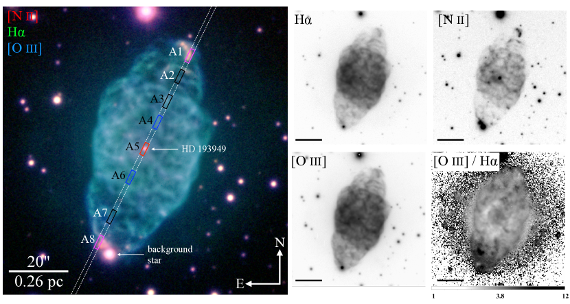
Figure 1: (left) NOT ALFOSC colour-composite image of NGC 6905 ([O iii] – blue, H$\alpha$ – green, [N ii]– red). The white dashed-line region represents the NOT ALFOSC slit at PA of 155^∘. The solid-line rectangles (0.75$\times$5 arcsec), labeled from A1 to A8, indicate our spectra extraction regions. The position of the CSPN (HD 193949) and a background star are indicated with arrows. (right) Individual H$\alpha$, [N ii] and [O iii] intensity images and line intensity [O iii]/H$\alpha$ ratio map. Each panel have the same FoV.

About 10 per cent of the central stars of planetary nebulae (CSPNe) are H-poor with strong and broad emission lines from He, C, N and O in their spectra. These spectral features resemble those typical in massive stars in their Wolf-Rayet (WR) phase (see Crowther, 2007) and can be classified following the same scheme (see Crowther et al., 1998; Acker & Neiner, 2003) as C-rich ([WC]), N-rich ([WN]) and with strong O emission lines ([WO]), with sub-classifications assigned depending on the ratio of the line strengths in their spectra. The most numerous [WR]-type stars are those of the carbon sequence, followed by the [WO]-types (see table 2 in Weidmann et al., 2020, and references therein), with a few cases of [WN]-types and transitional [WN/C]-types (e.g., Todt et al., 2010, 2013; Miszsalski et al., 2012).

Statistical analyses of PNe with [WR]-type CSPNe (hereinafter WRPN) have unveiled differences when compared to PNe with H-rich CSPNe. High-resolution spectroscopic observations have shown that WRPNe exhibit larger expansion velocities and present a higher degree of turbulence than non-WRPNe, very likely due to their higher wind mechanical luminosities or the presence of highly-collimated outflows (Gesicki et al., 2003; Medina et al., 2006; Rechy-García et al., 2017). WRPNe have also been found to have higher N and C abundances, suggesting that they are formed as a result of $\sim$4 M_⊙ stars (García-Rojas et al., 2013). It has also been suggested that there is a relation between the decrease in electron density with decreasing spectral subtype as a sign of evolutionary sequence from late to early [WC]-types (Acker et al., 1996; Górny & Tylenda, 2000). However, the N/O abundance ratio versus spectral type has shown that stars with different masses can evolve through the same [WC] state (Peña et al., 1998, 2001).

In Gómez-González et al. (2020, hereinafter Paper I), we started a series of works dedicated to a comprehensive characterisation of WRPNe. In Paper I we noted that statistical studies of WRPNe are helpful unveiling their properties as a population, but these do not provide the details that particular studies can offer us when combining multi-wavelength observations with theoretical predictions. Our analysis of the high-excitation WRPN NGC 2371 and its [WO1] CSPN WD 0722$+$295 presented in Paper I helped us to unveil its physical properties, origin and kinematical structure.

In this paper, we present a comprehensive multi-wavelength characterisation of NGC 6905 (PN G 061.4-09.5), a.k.a. the "Blue Flash Nebula" for its characteristic colours. NGC 6905 is a high-excitation WRPN with a clearly clumpy morphology (see Fig. 1), located at a distance of 2.7 kpc (Gaia Collaboration et al., 2020). It is composed of a central roundish cavity with angular radius $\sim$19 arcsec (0.25 pc) and a pair of extended V-shaped structures extending towards the NW and SE directions with a position angle (PA) of $\sim$160^∘ and with a total extension $\sim$80 arcsec (1 pc). These bipolar structures harbour a pair of low-ionization knots at their tips. These low-ionization features expand faster than the central regions of NGC 6905 with an inclination of 60^∘ with respect of the plane of the sky (Sabbadin & Hamzaoglu, 1982) and have been suggested to be responsible for giving this WRPN its bipolar morphology (Cuesta et al., 1993).

The CSPN of NGC 6905 has been classified as [WO]-type star. Due to the significant O vi emission lines, it has been classified as a [WO2]-subtype (Acker & Neiner, 2003). Spectroscopic studies in UV of NGC 6905 such as those presented by Keller et al. (2011, 2014) have allowed stellar atmosphere modeling of HD 193949 implying a $T_{\mathrm{eff}}$ in the range of 150–165 kK. These authors also found Ne to be overabundant with a mass fraction of 0.02.

This paper is organised as follows. In Section 2, we describe the observations used in this work. In Section 3, we present the analysis of the spectra and images. A discussion is presented in Section 4. Finally, our summary and conclusions are listed in Section 5.

2 OBSERVATIONS AND DATA PREPARATION

2.1 Nordic Optical Telescope

Optical images and spectra of NGC 6905 were obtained with the Alhambra Faint Object Spectrograph and Camera (ALFOSC) at the 2.5 m Nordic Optical Telescope (NOT) of the Observatorio del Roque de los Muchachos (ORM) in La Palma, Spain.

The images were obtained on 2009 July 21, using the H$\alpha$ ($\lambda_{\mathrm{c}}$=6563 Å and $\Delta\lambda$=33 Å), [N ii] ($\lambda_{\mathrm{c}}$=6584 Å and $\Delta\lambda$=36 Å) and [O iii] ($\lambda_{\mathrm{c}}$=5010 Å and $\Delta\lambda$=43 Å) narrow-band filters. Two images of 450 s were obtained in each filter. The images were processed using standard iraf routines (Tody, 1993) and are presented in Figure 1, together with a colour-composite picture and a [O iii]/H$\alpha$ ratio map.

NOT spectroscopic observations were carried out on 2020 July 26. The EEV 231–42 2K$\times$2K CCD was used, providing a pixel scale of 0.211 arcsec pixel^-1 and a field of view (FoV) of 7 arcmin. A spectrum at a position angle (PA) of 155^∘ was obtained using the grism #7, which covered the spectral range of 3650–7110 Å and a dispersion of $\sim$1.7 Å pixel^-1. The total observing time was of 2400 s, which was split into two exposures of 1200 s. We adopted a slitwidth of 0.75 arcsec, with spectral resolution of $\sim$5 Å. The seeing during the observations was $\sim$1 arcsec. The details of the spectroscopic observations are presented in Table1.

The spectra were also reduced and analyzed using standard iraf routines, which include bias subtraction and flat-fielding. The wavelength calibration was performed using HeNe arc lamps and the flux calibration by using the standard star Wolf 1346.

In order to study the ionization structure of NGC 6905, we have extracted spectra from different regions defined along the slit using the iraf task apall. We first extracted the 1D spectrum of the CSPN tracing the stellar continuum along the 2D spectrum. This information was then used as a reference to trace the nebular spectra along the 2D spectra, as these regions do not show continuum emission. The location of the extracted regions, labelled A1–A8, are shown in Figure 1, all of them with equal sizes of 0.75$\times$5 arcsec. The corresponding extraction region for HD 193619 is A5. Finally, we note that all extracted spectra were corrected for extinction by using the $c$(H$\beta$) value estimated from the Balmer decrement method with an intrinsic H$\alpha$/H$\beta$, H$\gamma$/H$\beta$ and H$\delta$/H$\beta$ ratios of 2.86, 0.45 and 0.25, respectively, which corresponds to mean values for $T_{\rm e}$ in the range 2000 K and 12,000 K and $n_{\rm e}$ between 100 cm^-3 and 1200 cm^-3 (see Osterbrock & Ferland, 2006) and using the reddening curve of Cardelli et al. (1989) with $R_{\mathrm{V}}$=3.1. The spectrum of HD 193949 is presented in Figure 2 and the spectra from different regions will be discussed in Section 3.3.

Table 1: Spectroscopic observing log.

Grating	Type	Name	Coordinates (J2000)		Exposure	Airmass
			R.A.	Dec.	time (s)
grism7	object	NGC 6905	20:22:22.6	20:06:15.5	2$\times$1200	1.15
	stds	Wolf 1346	20:34:21.2	25:03:34.4	6$\times$60	1.53
	arc	HeNe	–	–	2$\times$2	1.35
	flat	Halogen	–	–	10$\times$33.3	1.00
	bias	–	–	–	24$\times$0	–

2.2 IR data

In order to produce a consistent model of the nebular and dust properties of NGC 6905, we also need the infrared (IR) photometry of this WRPN. The necessary IR data were retrieved from the NASA/IPAC IR archive. Specifically, we retrieved archival IR images obtained from Spitzer, WISE, IRAS and Akari. With these, we can create a spectral energy distribution (SED) that covers the 5.8–160 $\mu$m spectral range. Details of the observations used here are listed in Table 2.

Table 2: IR observations of NGC 6905.

Telescope	Instrument	Band	Obs. date	Obs. ID.
		($\mu$m)	(yyyy-mm-dd)
Spitzer	IRAC	5.8, 8.0	2004-10-08	4421376
WISE		12, 22	2010-05-01	3056p196_ac51
IRAS	ISSA-II	60, 100	1992-04-22
Akari	FIS	140, 160	2000-01-01

Table 3: IR and radio photometric fluxes of NGC 6905.

Wavelength	Band	Flux	Error
range	($\mu$m)	(mJy)	(mJy)
Infrared	5.8	45	1
	8.0	165	1
	12	652	26
	22	3471	19
	60	7620	71
	100	7600	2800
	140	2730	280
	160	1920	560
	(cm)
Radio	6	63	10
	20	67	3

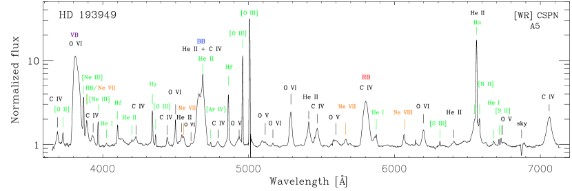
Figure 2: NOT ALFOSC spectrum of HD 193949, the CSPN of NGC 6905, extracted from region A5 defined in Fig. 1 (left panel). The most prominent broad WR features like the violet bump (VB) at $\sim\lambda 3820$ Å, the blue bump (BB) at $\sim\lambda 4686$ Å and the red bump (RB) at $\sim\lambda 5806$ Å are marked with their respective colours, whilst other WR features are indicated in black. Broad Ne lines of high ionization potential are indicated with orange labels, and the narrow nebular lines are labeled in green. The spectrum is shown normalized to the best-fit continuum spectrum. See table Table 4 for details.

IR photometric measurements were extracted from each image. We defined an extraction region that encompasses the nebular emission for each individual IR image. The corresponding photometric measurements were calculated adding up all the flux from the pixels within this region. Several background regions were selected from the vicinity of NGC 6905 with no contribution from the nebula, additionally we excised the contribution of background stars like the south-east star at the edge of the nebula. In Table 3 we list the photometric values and their errors. The errors account for the calibration uncertainty from each instrument as well as the standard deviation from the selected background regions. Details of this process can be found in Jiménez-Hernández et al. (2020, 2021) and Rubio et al. (2020) and will not be discussed here. We do not include the shorter wavelengths from Spitzer because of the presence of numerous background stars that hinders a proper photometry extraction.

Finally, photometric measurements obtained at radio frequencies were also included. Radio measurements at 1.4 and 4.85 GHz, that correspond to 20 and 6 cm, respectively, were also taken from the NASA/IPAC infrared archive, corresponding to the National Radio Astronomy Observatory (NRAO) Very Large Array (VLA) survey and the NRAO Green Bank telescope (GBT), respectively (see also Hajduk et al., 2018). The radio measurements are also listed in Table 3.

3 ANALYSIS

The NOT ALFOSC spectrum of HD 193949 presented in Figure 2 corroborates its [WR] nature with the clear presence of the broad features at $\sim$4686 Å  and $\sim$5806 Å, the so-called blue and red bumps (hereinafter BB and RB), together with other WR features. The CSPN of NGC 6905 also exhibits the broad O vi feature at $\sim$3820 Å  (hereinafter the violet bump or simply VB), which has been used to classify this object as part of the oxygen sequence (Acker & Neiner, 2003). Additionally, twenty one WR emission lines can be spotted in the ALFOSC spectrum at different wavelengths between 3680 Å and 7060 Å, plus several high-excitation Ne lines, which have never been discussed before. Several contributing narrow emission lines of nebular origin (non-stellar) are also labeled on the spectrum. All the ions responsible for the broad emission lines displayed in the spectrum of HD 193949 are listed in Table 4. Most of the observed wavelengths of the ions analysed here were consulted in the National Institute for Standards and Technology (NIST) Atomic Spectra Database.

Previous authors have developed a methodology to sub-classify [WR]-type CSPNe using the line fluxes and/or the equivalent widths (EW) of the broad spectral emission features (e.g., Acker & Neiner, 2003; Crowther et al., 1998). For this, we need to calculate the line fluxes for all the WR features in the spectrum; we note that some broad features are usually the result of blends of stellar broad features with some contribution from nebular lines. Although minor, these need to be taken into account. To help us disentangle the presence from the contributing nebular lines to the WR bumps, we applied the multi-Gaussian fitting technique discussed in length in Paper I. This method allows us to assess the contribution from nebular lines (e.g.: [Ar iv] $\lambda 4711$ and He ii $\lambda 4686$ in the BB). We give a brief description in the following.

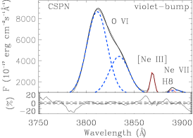
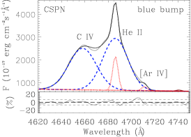
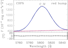
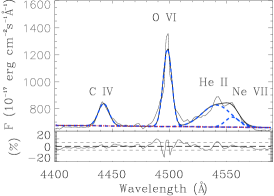
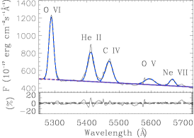
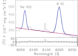
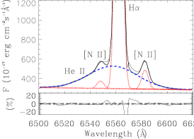
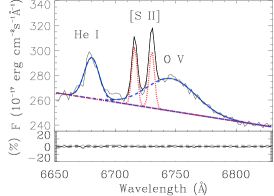
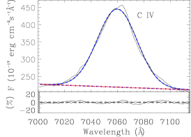
Figure 3: Multicomponent Gaussian fits to the bumps and other WR features of the CSPN on NGC 6905: VB (top left); BB (top center) and RB (top right). The rest of the panels show other WR features and high ionization Ne emission lines (see Fig. 2). The blue dashed lines represents the fits to the broad WR features and the red dotted-lines the narrow nebular emission. The sum is shown in black. The fitted continuum is shown by the dashed straight line. The residuals are shown at the bottom of each panel (in per cent). The results are listed in Table 4.

3.1 Line fluxes of the CSPN HD 193949

Table 4: Parameters of the WR features in the optical spectrum of the CSPN of NGC 6905.

ID	Nature	Ion	$\lambda_{0}$	$\chi$	$\lambda_{\mathrm{c}}$	$F^{\dagger}$	FWHM	$EW$	SNR	$F_{\mathrm{\lambda}}/F_{\mathrm{RB}}$	$EW_{\mathrm{\lambda}}/EW_{\mathrm{RB}}$
			(Å)	(eV)	(Å)	($10^{-14}$ erg cm-2 s-1)	(Å)	(Å)		($F_{\mathrm{RB}}=100$)	($F_{\mathrm{RB}}=100$)
(1)	(2)	(3)	(4)	(5)	(6)	(7)	(8)	(9)	(10)	(11)	(12)
VB
1	WR	O vi	3811	138.1	3811.0	206.99$\pm$0.46	24.8	245.9$\pm$1.3	43.6	572.74$\pm$2.29	279.37$\pm$0.15
2	WR	O vi	3834	138.1	3834.0	90.25$\pm$0.36	23.9	102.7$\pm$0.6	43.6	249.72$\pm$1.30	116.69$\pm$0.19
BB
3	WR	C iv	4658	64.5	4658.0	53.95$\pm$0.59	27.8	77.1$\pm$1.1	20.2	149.28$\pm$1.71	87.55$\pm$0.86
4	WR	He ii	4686	24.6	4686.0	61.52$\pm$0.58	25.4	90.4$\pm$1.2	20.2	170.23$\pm$1.70	102.71$\pm$0.94
5	Neb	He ii	4686	24.6	4686.1	8.62$\pm$0.24	5.4	12.7$\pm$0.4	20.2	23.85$\pm$0.67	14.39$\pm$0.45
6	Neb	[Ar iv]	4711		4711.0	1.05$\pm$0.19	5.4	1.6$\pm$0.3	20.2	2.91$\pm$0.53	1.80$\pm$0.32
RB
7	WR	C iv	5806	64.5	5802.8	36.14$\pm$0.12	37.4	88.0$\pm$0.4	65.5	100.00$\pm$0.47	100.00$\pm$0.03
other lines
8	WR	C iv	3689	64.5	3689.0	5.06$\pm$0.20	14.4	5.7$\pm$0.2	43.6	14.00$\pm$0.56	6.50$\pm$0.22
9	WR	C iv	3933	64.5	3932.4	3.19$\pm$0.19	18.1	4.2$\pm$0.2	43.6	8.83$\pm$0.53	4.73$\pm$0.25
10	WR	He ii	4200	24.6	4200.6	1.29$\pm$0.17	17.4	1.8$\pm$0.2	43.6	3.57$\pm$0.47	2.04$\pm$0.25
11	WR	C iv	4227	64.5	4226.7	2.96$\pm$0.18	18.9	4.2$\pm$0.2	43.6	8.19$\pm$0.50	4.72$\pm$0.26
12	WR	C iv	4440	64.5	4442.8	1.95$\pm$0.28	11.0	2.9$\pm$0.4	20.2	5.40$\pm$0.77	3.30$\pm$0.45
13	WR	O vi	4500	138.1	4498.1	5.48$\pm$0.27	8.9	8.2$\pm$0.4	20.2	15.16$\pm$0.75	9.34$\pm$0.43
14	WR	He ii	4541	24.6	4541.0	5.19$\pm$0.45	29.9	7.8$\pm$0.7	20.2	14.36$\pm$1.25	8.89$\pm$0.73
15	WR	C iv	4789	64.5	4789.2	1.99$\pm$0.33	21.4	3.4$\pm$0.6	20.2	5.51$\pm$0.91	3.84$\pm$0.62
16	WR	O v	4933	113.9	4933.1	4.87$\pm$0.38	30.3	8.7$\pm$0.7	20.2	13.48$\pm$1.05	9.92$\pm$0.74
17	WR	O v	5100	113.9	5100.0	3.60$\pm$0.41	41.5	6.9$\pm$0.8	20.2	9.96$\pm$1.14	7.84$\pm$0.86
18	WR	O vi	5166	138.1	5166.5	0.52$\pm$0.06	11.4	1.0$\pm$0.1	20.2	1.44$\pm$0.17	1.15$\pm$0.13
19	WR	O vi	5290	138.1	5288.9	13.13$\pm$0.09	17.3	26.4$\pm$0.2	66.8	36.33$\pm$0.28	29.94$\pm$0.09
20	WR	He ii	5412	24.6	5411.8	8.49$\pm$0.09	23.6	17.9$\pm$0.2	66.8	23.49$\pm$0.26	20.34$\pm$0.13
21	WR	C iv	5470	64.5	5468.6	6.89$\pm$0.10	26.6	114.9$\pm$0.2	66.8	19.07$\pm$0.26	16.91$\pm$0.15
22	WR	O v	5600	113.9	5595.0	2.59$\pm$0.07	35.5	5.9$\pm$0.2	65.5	7.17$\pm$0.28	6.72$\pm$0.22
23	WR	O vi	6200	138.1	6198.5	3.35$\pm$0.08	19.0	10.2$\pm$0.3	43.3	9.27$\pm$0.22	11.61$\pm$0.24
24	WR	He ii	6406	24.6	6406.0	0.63$\pm$0.03	11.8	2.2$\pm$0.2	43.3	1.74$\pm$0.14	2.51$\pm$0.20
25	WR	He ii	6560	24.6	6557.7	10.95$\pm$0.07	44.5	36.7$\pm$0.4	43.3	30.30$\pm$0.35	41.69$\pm$0.29
26	WR	O v	6740	113.9	6746.3	1.33$\pm$0.10	47.9	5.3$\pm$0.4	43.3	3.68$\pm$0.26	6.01$\pm$0.40
27	WR	C iv	7060	64.5	7059.9	8.54$\pm$0.04	35.4	39.0$\pm$0.3	57.9	23.63$\pm$0.18	44.31$\pm$0.15
special lines††
28	stellar emission	Ne vii	4555	207.3	4552.5	1.14$\pm$0.30	14.4	1.7$\pm$0.5	20.2	3.15$\pm$0.83	1.96$\pm$0.51
29	stellar emission	Ne vii	5666	207.3	5665.4	1.63$\pm$0.07	20.4	3.8$\pm$0.2	65.5	4.51$\pm$0.19	4.36$\pm$0.17
30	stellar emission	Ne viii	6068	239.1	6065.9	1.51$\pm$0.07	12.1	4.2$\pm$0.2	43.3	4.18$\pm$0.19	4.82$\pm$0.21

Notes. (1) Identification number; (2) nature of the contributing emission line: WR (broad/stellar) or nebular (narrow); (3) ion; (4) rest wavelength in Å; (5) Ionisation potential [eV]; (6) observed centre of the line; (7) flux [$10^{-14}$ erg cm^-2 s^-1]; (8) full width at half maximum (FWHM) [Å]; (9) equivalent width (EW) [Å]; (10) continuum signal-to-noise ratio (SNR) closest to the feature; (11) line fluxes normalized to that of the RB. The ratio has been computed adopting $F$(RB)=100. (12) EW normalized to that of the RB, adopting $EW$(RB)=100. Special lines^†† correspond to high ionization Ne lines from stellar emission origin (Werner et al., 2007). ^† Only the statistical errors, determined with equations 1 and 2, are shown in this table.

Table 5: Diagnostic criteria to classify HD 193949 as a [WR]-type CSPN.

Criteria	[WO1]	[WO2]	[WO3]	WRPN	Classification
(1)	(2)	(3)	(4)	(5)	(6)
Acker & Neiner (2003)
$F_{\text{O{\,vi}\ 3822}}/F_{\text{RB}}$	$>1400$	1000$\pm$200	250$\pm$40	822.5$\pm$2.6	[WO2]
$F_{\text{C{\,iv}\ 4650}}/F_{\text{RB}}$	300$\pm$100	270$\pm$60	23$\pm$2	149.3$\pm$1.7	[WO2]
$F_{\text{C{\,iv}\ 4686}}/F_{\text{RB}}$	500$\pm$200	300$\pm$30	130$\pm$30	170.2$\pm$1.7	[WO2–3]
$F_{\text{O{\,vi}\ 5290}}/F_{\text{RB}}$†	$>80$	48$\pm$2	20$\pm$5	36.3$\pm$0.3	[WO2–3]
$F_{\text{C{\,iv}\ 5412}}/F_{\text{RB}}$	45$\pm$15	20$\pm$4	15$\pm$4	23.5$\pm$0.3	[WO2]
$F_{\text{C{\,iv}\ 5470}}/F_{\text{RB}}$	35$\pm$5	23$\pm$2	14$\pm$2	19.1$\pm$0.3	[WO2]
$F_{\text{Ne{\,vii}\ 5666}}/F_{\text{RB}}$†	$>25$	10:	8$\pm$6	4.5$\pm$0.2	[WO2–3]
$F_{\text{Ne{\,viii}\ 6068}}/F_{\text{RB}}$†	20$\pm$8	6$\pm$1	2$\pm$1	4.18$\pm$0.2	[WO2–3]
$F_{\text{O{\,v}\ 6740}}/F_{\text{RB}}$	presence	–	–	3.7$\pm$0.3	[WO1]
$F_{\text{C{\,iv}\ 7060}}/F_{\text{RB}}$	35$\pm$20	18$\pm 4$	15$\pm$4	23.6$\pm$0.2	[WO1–2]
FWHM of C iv $\lambda\lambda 5806$[Å]	33$\pm$5	32$\pm$3	37$\pm$6	37.4	[WO1–3]
Crowther et al. (1998)
log$(EW_{\text{O{\,vi}3820}}/EW_{\text{O{\,v}5590}})$	$\geq 1.1$	0.6–1.1	0.25–0.6	1.58	[WO1]
log$(EW_{\text{O{\,vi}3820}}/EW_{\text{C{\,iv}5806}})$	$\geq 0.2$	$\geq 0.2$	$-1$–0.2	0.46	[WO1–2]
log$(EW_{\text{Ne{\,vii}5666}}/EW_{\text{O{\,v}5590}})$†	$\geq 0.0$	$\leq 0.0$	$<<0.0$	$-0.19$	[WO2]
FWHM of C iv $\lambda\lambda 5806$ [Å]	40$\pm$10	160$\pm$20	90$\pm$30	37.4	[WO1]

^†Note that we here identify the $\lambda 5290$ emission line as O vi and not as C vi; the $\lambda 5666$ as Ne vii and not as O vii; and the $\lambda 6068$ as Ne viii and not as O viii, as previously defined (see Crowther et al., 1998; Acker & Neiner, 2003). However, according to spectral observations these updated criteria remains as valid as before (see Werner et al., 2007), and given its importance for classification, the re-identification is worth clarifying for future use. See text for details.

The WR features in the spectrum of the CSPN HD 193949 (Figure 2) were decomposed into their individual emission lines by following the multi-Gaussian approach (discussed in length in Gómez-González et al., 2020). In brief, the method consists of fitting the individual WR features with multi-Gaussian components using a tailor-made code that uses the idl routine lmfit which performs a non-linear least squares fit of a function with an arbitrary number of parameters by using the Levenberg-Marquardt algorithm (Press et al., 1992). The resultant fits to each broad spectral feature give us the line fluxes ($F$), central wavelength ($\lambda_{\mathrm{c}}$), full width at half-maximum (FWHM) and EW from the contributing lines from stellar and nebular origin. Table 4 resumes our findings.

Examples of multi-Gaussian fitting to several WR features in HD 193949 are illustrated in Figure 3. In order of increasing ionization potential, the WR features detected are: He ii $\lambda\lambda$4200, 4541, 4686, 5412, 6406, 6560; C iv $\lambda\lambda$3689, 3933, 4227, 4440, 4658, 4789, 5470, 5806, 7060; O v $\lambda\lambda$4933, 5100, 5600, 6740 and O vi $\lambda\lambda$3811, 3834, 4500, 4604, 5166, 5290, 6200. We highlight the presence of three Ne broad emission lines: Ne vii $\lambda\lambda 4555,5666$ and Ne viii $\lambda 6068$, of stellar origin according to Werner et al. (2007). These lines are discussed in the following sections.

We found that the VB is composed of two broad emission lines of O vi $\lambda\lambda 3811,3834$, with negligible contribution of [Ne iii] and Ne vii at its red wing (see Fig. 3 top left panel). The BB, composed by the broad He ii $\lambda 4686$ and C iv $\lambda 4658$ features, has some contribution from nebular lines of He ii and [Ar iv] (Fig. 3 top middle panel). The RB is fitted by a single broad line at $\sim\lambda 5806$ Å, from the blended components of C iv $\lambda\lambda 5801,5812$ (Fig. 3 top right panel). Notice that they all correspond to broad emission lines (FWHM$>$5.4 Å; see Table 4, column 8), according to their WR nature.

The statistical errors of the emission lines were determined as the 1-$\sigma$ deviation, $\sigma_{l}$, on each measured flux of the emission line using the expressions from Tresse et al. (1999):

$$\sigma_{l}=\sigma_{c}D\sqrt{2N_{\rm pix}+\frac{EW}{D}},$$ (1)

and for the EW:

$$\sigma_{EW}=\frac{EW}{F}\sigma_{c}D\sqrt{\frac{EW}{D}+2N_{\rm pix}+\left(\frac{EW}{D}\right)^{2}},$$ (2)

where $D$=1.7 Å pixel^-1 is the spectral dispersion (for NOT ALFOSC), $\sigma_{c}$ is the mean standard deviation per pixel of the continuum and $N_{\rm pix}$ is the number of pixels covered by the feature.

In Table 4 we also list what we call "special lines", corresponding to high ionization potential Ne lines (see column 5) from presumably stellar emission origin. Before Werner et al. (2007), the Ne viii emission line at $\sim$6068 Å, with a ionization potential of 239.1 eV, was previously identified as a non-stellar ultra-high ionization O feature, O viii, with a much higher ionization potential of 871.4 eV. This ion supposedly formed in shock wind regions.

The same applied to other spectral features like O viii $\lambda 4340$ now identified as Ne viii; C vi $\lambda 4500$ now identified as O vi; O vii $\lambda 4555$ now identified as Ne vii; C v $\lambda 4945$ now identified as N v; C vi $\lambda 5290$ now identified as O vi and O vii $\lambda 5665$ now identified as Ne vii. We note that although the presence of X-ray-emitting gas is invoked in low $T_{\mathrm{eff}}$ CSPN to explain the ultrahigh-ionization O features (see, e.g. the case of IC 4593; Herald & Bianchi, 2011; Toalá et al., 2020), this might not be the case for hot WRPN. Furthermore, Werner et al. (2007) showed that the mere presence of Ne vii and Ne viii puts a strict lower limit of $T_{\mathrm{eff}}\approx 150$ kK.

In Table 4 we present the flux, FWHM, EW, as well as the parameters $F_{\mathrm{\lambda}}/F_{\mathrm{RB}}$ adopting $F_{\mathrm{RB}}=100$ and $EW_{\mathrm{\lambda}}/EW_{\mathrm{RB}}$ adopting $EW_{\mathrm{RB}}=100$, that are used as a classification criteria for CSPNe, according with Acker & Neiner (2003) and Crowther et al. (1998). The mere presence of the strong O vi broad emission line $\sim\lambda 3820$ Å, the VB in the CSPN spectrum of NGC 6905 (see Fig. 2), suggests a [WO]-type classification. Moreover, the presence of high-ionized Ne lines constrains it to a very early-type (e.g Werner et al., 2007). A classification of CSPNe later than [WO2]-subtypes can be safely discarded since they do not display neither Ne vii nor Ne viii in their spectra. Besides, later [WO]-subtypes, like [WO4], present weaker O vi and C iv intensities, in general. Also, any [WC] fingerprint (early or later) is also discarded: C iii lines, expected in [WCL]-subtypes, are absent in our spectrum, and in the classification schemes by Acker & Neiner (2003) and Crowther et al. (1998), [WCE]-subtypes do not display a strong VB, by definition. It is worth to explicitly mention that we also did not detect any broad N lines, which also rules out any [WN]-subtype or transitional stages [WN/C].

In order to quantitatively classify the CSPN of NGC 6905 as [WO]-type, Table 5 summarizes the values of the main parameters among the [WO]-subtypes in which our [WR] star is expected to be ([WO1], [WO2] and [WO3]), according to the lines present in our spectrum. The spectrum of HD 193949 suggest a [WO2]-subtype based on the Acker & Neiner (2003) criteria, whilst the Crowther et al. (1998) scheme suggest a [WO1]-subtype. In conclusion, we classified the CSPN of NGC 6905 as a [WO]-type, specifically an early one, between [WO1] and [WO2]-subtype.

3.2 NLTE analysis of HD 193949

We have analysed UV and optical spectra by means of the most updated version (2021 January 24) of the non-local thermodynamic equilibrium (NLTE) stellar atmosphere code Potsdam Wolf-Rayet (PoWR; Gräfener et al., 2002; Hamann & Gräfener, 2004) in order to infer the stellar parameters of HD 193949. Details of the computing scheme can be found in Todt et al. (2015).

Available UV Far Ultraviolet Spectroscopic Explorer (FUSE) and Hubble Space Telescope (HST) Space Telescope Imaging Spectrograph (STIS) observations of HD 193949 were retrieved from the Mikulski Archive for Space Telescopes (MAST). The UV observations were analysed in conjunction with the optical NOT ALFOSC spectra with the PoWR stellar atmosphere code. The FUSE observation corresponds to Obs. ID. a1490202000 (PI: F. Bruhweiler) and were obtained on 2000 August 11 with the LWRS aperture for a total exposure time of 9487 s. The HST STIS data were taken on 1999 June 29 and correspond to Obs. ID. o52r01010 (NUV-MAMA) and o52r01020 (FUV-MAMA), each with an exposure time of 802 s (PI: A. Boggess) and taken with the time-tag mode with the $52\times 0.5\arcsec$ aperture. The FUV-MAMA observation was performed with the G140L grating at a central wavelength of 1425 Å, and the NUV-MAMA with the G230L grating at a central wavelength of 2376 Å. We notice that there might be a problem with the background subtraction for the FUV-MAMA observation, as the flux at the centre of the interstellar Lyman-$\alpha$ absorption line as well as the absorption trough of the C iv resonance doublet does not reach zero.

As the typical emission-line spectra of WR-type stars are predominantly formed by recombination processes in their dense stellar winds, the continuum-normalized spectrum shows a useful scale-invariance: for a given stellar temperature ($T_{\star}$) and chemical composition, the EW of the emission lines depend in first approximation only on the volume emission measure of the wind normalized to the area of the stellar surface. An equivalent quantity, which has been introduced by Schmutz et al. (1989), is the transformed radius $R_{\mathrm{t}}$ defined as:

$$R_{\mathrm{t}}=R_{\star}\left[\frac{\text{v}_{\infty}}{2500~{}\mathrm{km}~{}\mathrm{s}^{-1}}\bigg{/}\frac{\dot{M}\sqrt{D}}{10^{-4}\mathrm{M}_{\odot}~{}\mathrm{yr}^{-1}}\right]^{2/3}~{}.$$ (3)

Different combinations of stellar radii ($R_{\star}$) and mass-loss rates ($\dot{M}$) can thus lead to the same emission-line strengths. This invariance also includes the micro-clumping parameter $D$, which is defined as the density contrast between wind clumps and a smooth wind of the same $\dot{M}$. Hence, empirically derived $\dot{M}$ depend on the adopted value of $D$. The parameters of our best fitting model for the stellar atmosphere of HD 193949 obtained with PoWR are listed in Table 6. All of our calculations were performed adopting a stellar mass of $M_{\star}$=0.6 M_⊙, which is the typical value for an evolved low-mass star (see Miller Bertolami, 2016; Kepler et al., 2016, and references therein). The actual mass has only little impact on the spectrum of the central star, as the spectrum is formed in the wind. The stellar temperature $T_{\star}$, defined at $\tau_{\mathrm{Ross}}$=20, is constrained by the relative strength of the emission lines, mainly by the ratio of the O vi vs. the O v emission lines. The best fit is achieved with $T_{\star}=140^{\,+5}_{\,-2}$ kK.

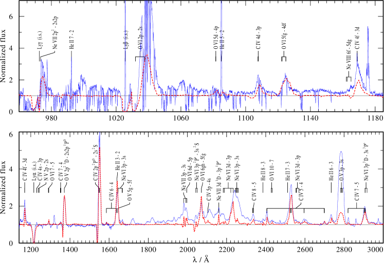
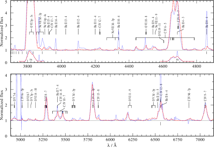
Figure 4: PoWR model (red dashed line) compared with the UV and optical observations of the CSPN HD 193949 (blue): FUSE (1st panel), HST STIS (2nd panel) and optical ALFOSC (3rd and 4th panel). The model spectra are convolved with a Gaussian to match the instrument’s spectral resolution. The black lines below the continuum in the 3rd and 4th panel mark the nebular Balmer lines. See text for details.

Table 6: Parameters of HD 193949, the CSPN of NGC 6905, obtained with PoWR.

Parameter	Value	Comment
$d$ [kpc]	$2.7\pm 0.2$	Bailer-Jones et al. (2021)
$E(B-V)$ [mag]	$0.20\pm 0.05$	SED fit
$M_{\star}$ [M⊙]	0.6	adopted
$T_{\star}$ [kK]	$140^{+5}_{-2}$	Defined at $\tau_{\text{Ross}}=20$
$\log(L_{\star}$/L${}_{\odot})$	3.9$\pm 0.1$
$R_{\star}$ [R⊙]	$0.15\pm 0.02$	stellar radius
$\log R_{\text{t}}$ [R⊙]	$0.75\pm 0.05$	transformed radius (see Eq. 3)
$\dot{M}/$M⊙ yr-1	$(1.1\pm 0.3)\times 10^{-7}$
$\text{v}_{\infty}$ [km s-1]	$2000\pm 100$
$D$	10	adopted density contrast
$\beta$	1	$\beta$-law exponent
Chemical abundances (mass fraction)
H	$<0.05$	upper limit
He	$0.55\pm 0.05$
C	$0.35\pm 0.05$
N	$<6.9\times 10^{-5}$	$1/10$ solar, upper limit
O	$0.08\pm 0.01$
Ne	$0.02\pm 0.01$
Fe	$1.4\times 10^{-3}$	solar, adopted

With $T_{\star}$ and $R_{\mathrm{t}}$ determined from the continuum-normalized spectra, we can fit the synthetic SED to Gaia eDR3 photometry (Gaia Collaboration et al., 2020) and the flux-calibrated UV spectra to estimate $L_{\star}$ and $E(B-V)$. Taking into account the loss of flux from the CSPN due to the long-slit spectroscopic observations, the stellar luminosity is $L_{\star}$=7600 L_⊙ for the photogeometric distance of 2.7 kpc (Bailer-Jones et al., 2021). Our fit implies a reddening of $E(B−V)=0.21$ mag using the extinction law by Cardelli et al. (1989), consistent with value derived by previous authors (see Keller et al., 2014). We note, however, that such model requires a higher value of $R_{\mathrm{V}}$=3.8 that suggests that the extinction towards HD 193949 is higher due to the presence of different dust compositions along the line of sight (see, e.g., Todt et al., 2010).

The spectral fit to the blue edges of the P-Cygni line profiles resulted in a terminal wind velocity of $\text{v}_{\infty}=2000$ km s^-1 by adopting a $\beta$-law with $\beta=1$. Additional line broadening by microturbulence is also included in our models. From the shape of the line profiles we estimate a value of about $100\,\mathrm{km}\,\mathrm{s}^{-1}$. From Equation (3) we obtained a mass-loss rate of $\dot{M}=1.1\times 10^{-7}$ M_⊙ yr^-1 adopting a density contrast of $D$=10, which is a typical value also found for other [WC]-CSPNe (e.g., Marcolino et al., 2007; Todt et al., 2008). We achieve a similar fit quality also with a lower value of $D=4$ and $\log(R_{\mathrm{t}}/R_{\odot})=0.8$, while even smaller values of $D$, e.g., a smooth wind with $D=1$, yield too strong electron scattering line wings. For larger values of $D$ the fit quality is worse.

To determine the C and He abundances we mainly focused on the "diagnostic line pair" He ii $\lambda$5411 & C iv $\lambda$5471 (Todt et al., 2006). Both features are formed at the same region in the wind, hence their relative strength is less sensitive to temperature and $\dot{M}$. For the hot [WC] and [WO] stars an abundance ratio of about He:C $\approx$ 60:30 yields approximately equal strength for both emission features, as it is observed. For the O abundance we used primarily the O vi multiplet at $\approx$ 5290 Å, as this line is less sensitive to $T_{\star}$ and $R_{\mathrm{t}}$ and more sensitive to the O abundance. The spectrum of HD 193949 displays many Ne vi and Ne vii lines in the UV and optical. With the inferred Ne abundance of about 2 per cent by mass we got a reasonable fit to most of these lines. However, we also note the presence of Ne viii features around 1162 Å and 1165 Å (see Fig. 4, top panel), as described in Werner et al. (2007). While these lines are in absorption in the model, it appears that they are in emission in the FUSE observation. There is also the emission feature at 6068 Å in the NOT spectrum, which might be also attributed to Ne viii. However, our model is not hot enough to produce this potential Ne viii emission line. For our object, this would require a stellar temperature above 170 kK, which is excluded by the presence of the observed O v lines. This emission feature has been reported to appear in the spectrum of other hot CSPNe such as NGC 2371 (see Paper I) and PC 22 (Sabin et al. in prep.). It seems that there is no N line present in the UV and optical spectra: the N v resonance doublet is not detectable and the emission features around 4604 Å and 4933 Å, which are also seen in hot WN stars, originate from O vi and O v respectively. Therefore, we estimate the N fraction to be at most 1/10 of the solar value. For the H abundance we can only give an upper limit too, as stellar Balmer lines would be blended with the corresponding He ii lines from the Pickering series and nebular H emission lines. We find that a H mass fraction below 5 per cent would escape detection. In the absence of strong spectral lines from the iron group elements and with regard to the limited quality of the UV spectra we could not determine an iron abundance and adopted instead the solar value. Figure 4 shows the comparison between the best fitting PoWR model for HD 193949 and its FUSE, HST STIS and NOT optical spectra, respectively.

Our analysis yields similar values for the abundances and stellar parameters reported in previous works (Marcolino et al., 2007; Keller et al., 2014), although this work is based on a measured distance, hence we can give now a reliable estimate for $L$ and $\dot{M}$. We note that our C abundance is lower than that derived by Keller et al. (2014), who inferred the abundances from the UV spectra only, while we fitted also the optical spectrum.

3.3 Physical properties of NGC 6905

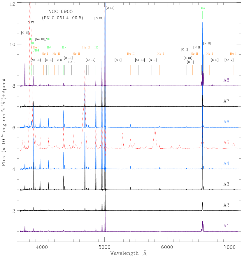
Figure 5: NOT ALFOSC spectra from the extracted regions A1–A8 in NGC 6905. The main emission lines are labeled. For the sake of clarity, H-Balmer lines are indicated in green, He lines in orange and the rest of the lines in black. The spectrum of the CSPN HD 19394 (A5) is shown in red dotted line in the middle for reference. The colours of the spectra were coded as the extraction apertures indicated in Fig. 1. To avoid overlap, the spectra are shifted upwards (A6–A8) and downwards (A4–A1) with respect to the spectrum of the CSPN by appropriate amounts (its continuum level corresponds to its aperture number). Thereby, the "onion-like" ionization structure of the object can be clearly appreciated. See Table 7 for details of the present lines and their fluxes.

Table 7: De-reddened line fluxes relative to H$\beta$=100. The location of the apertures A1–A8 are shown in Fig. 1 and their sizes are indicated. Their spectra are shown in Fig. 5.

$\lambda_{0}$	line	A1	A2	A3	A4	A6	A7	A8
		(5 arcsec)	(5 arcsec)	(5 arcsec)	(5 arcsec)	(5 arcsec)	(5 arcsec)	(5 arcsec)
3727.0	[O ii]	222$\pm$12	…	21.1$\pm$1.1	18.8$\pm$3.9	9.8$\pm$2.9	64.0$\pm$3.4	490$\pm$27
3797.9	H10	…	…	5.4$\pm$0.3	5.4$\pm$1.5	4.0$\pm$1.9	…	…
3835.4	H9	…	…	6.4$\pm$0.3	6.3$\pm$1.3	20.3$\pm$2.2	…	…
3868.8	[Ne iii]	108$\pm$6	113$\pm$6	94.3$\pm$4.7	90$\pm$6	70.4$\pm$4.3	134$\pm$7	170$\pm$11
3888.6	He i	18.9$\pm$2.0	16.7$\pm$3.0	12.5$\pm$0.6	12.6$\pm$1.5	12.0$\pm$1.4	11.8$\pm$0.8	20.5$\pm$3.8
3967.5	[Ne iii]	45.6$\pm$2.3	46.3$\pm$2.3	42.9$\pm$4.9	40.1$\pm$2.5	35.0$\pm$2.2	54.1$\pm$2.9	56$\pm$4
4026.2	He i	…	…	1.9$\pm$0.5	1.6$\pm$0.3	1.3$\pm$0.3	…	…
4070.0	[S ii]	…	…	1.9$\pm$0.4	1.5$\pm$0.3	1.3$\pm$0.3	…	4.9$\pm$1.7
4101.7	H$\delta$	25.7$\pm$1.3	25$\pm$10	24.8$\pm$1.6	25.3$\pm$1.4	25.9$\pm$1.4	25.1$\pm$1.3	25.0$\pm$1.9
4200.0	He ii	…	…	1.7$\pm$0.3	1.6$\pm$0.2	2.0$\pm$0.3	3.0$\pm$0.4	…
4267.3	C ii	…	…	…	1.1$\pm$0.2	0.6$\pm$0.2	…	…
4340.5	H$\gamma$	46.2$\pm$3.6	47.6$\pm$3.3	45.8$\pm$2.3	45.8$\pm$2.3	45.7$\pm$2.3	47$\pm$5	45.8$\pm$2.4
4363.2	[O iii]	13.8$\pm$2.1	14.4$\pm$1.9	12.4$\pm$0.7	11.0$\pm$0.6	10.2$\pm$0.6	18.3$\pm$2.9	16.8$\pm$1.2
4471.5	He i	2.7$\pm$1.5	…	1.0$\pm$0.2	1.2$\pm$0.2	0.7$\pm$0.1	…	3.9$\pm$0.8
4541.0	He ii	…	…	3.0$\pm$0.3	3.0$\pm$0.2	3.3$\pm$0.3	2.7$\pm$1.0	2.3$\pm$1.0
4686.0	He ii	56.8$\pm$3.0	96$\pm$5	99$\pm$5	100$\pm$5	106$\pm$5	97$\pm$5	48.0$\pm$2.5
4711.4	[Ar iv]	…	4.8$\pm$1.3	5.4$\pm$0.3	5.8$\pm$0.3	7.7$\pm$0.4	4.3$\pm$1.2	1.9$\pm$0.8
4740.2	[Ar iv]	…	…	4.1$\pm$0.3	4.3$\pm$0.3	5.8$\pm$0.3	2.4$\pm$1.1	2.2$\pm$0.9
4861.4	H$\beta$	100	100	100	100	100	100	100
4958.9	[O iii]	347$\pm$18	385$\pm$20	353$\pm$18	310$\pm$16	249$\pm$13	507$\pm$27	391$\pm$20
5006.8	[O iii]	1040$\pm$60	1170$\pm$60	1050$\pm$50	930$\pm$50	743$\pm$38	1510$\pm$90	1160$\pm$60
5200.0	[N i]	3.6$\pm$0.9	…	…	…	…	…	2.4$\pm$0.6
5411.0	He ii	4.7$\pm$1.0	7.1$\pm$1.0	7.6$\pm$0.4	7.6$\pm$0.4	8.1$\pm$0.4	7.6$\pm$0.7	…
5517.7	[Cl iii]	1.5$\pm$0.9	…	0.9$\pm$0.1	0.7$\pm$0.1	0.7$\pm$0.1	1.3$\pm$0.7	…
5537.9	[Cl iii]	1.1$\pm$0.9	…	0.6$\pm$0.1	0.6$\pm$0.1	0.5$\pm$0.1	…	…
5754.6	[N ii]	3.9$\pm$0.9	…	0.2$\pm$0.1	…	…	…	4.6$\pm$0.5
5875.6	He i	9.9$\pm$1.1	6.2$\pm$1.4	3.7$\pm$0.2	3.6$\pm$0.2	2.5$\pm$0.2	5.8$\pm$1.0	9.3$\pm$0.7
6300.0	[O i]	23.6$\pm$1.7	…	…	…	…	…	15.3$\pm$1.0
6312.1	[S iii]	2.3$\pm$1.4	2.8$\pm$1.5	2.2$\pm$0.2	2.1$\pm$0.2	1.9$\pm$0.2	2.8$\pm$1.1	2.8$\pm$0.7
6363.8	[O i]	8.1$\pm$1.3	…	…	…	…	…	5.0$\pm$0.7
6406.0	He ii	…	…	0.3$\pm$0.1	0.3$\pm$0.1	0.4$\pm$0.1	…	…
6548.1	[N ii]	60.6$\pm$3.1	7.1$\pm$1.2	3.4$\pm$0.2	2.7$\pm$0.2	1.9$\pm$0.2	9.6$\pm$1.1	67.9$\pm$3.4
6562.8	H$\alpha$	283$\pm$15	285$\pm$15	260$\pm$13	271$\pm$14	279$\pm$14	278$\pm$15	245$\pm$12
6583.5	[N ii]	187$\pm$10	21.9$\pm$1.5	9.8$\pm$0.5	7.8$\pm$0.4	5.0$\pm$0.3	27.6$\pm$1.5	208$\pm$10
6678.2	He i	1.7$\pm$0.9	1.7$\pm$1.1	1.4$\pm$0.1	1.4$\pm$0.1	…	1.4$\pm$0.8	2.0$\pm$0.5
6716.4	[S ii]	17.4$\pm$1.2	5.4$\pm$1.1	2.7$\pm$0.2	2.2$\pm$0.1	1.5$\pm$0.1	7.0$\pm$0.9	24.8$\pm$1.3
6730.8	[S ii]	15.5$\pm$1.1	4.2$\pm$1.1	2.4$\pm$0.2	2.0$\pm$0.1	1.2$\pm$0.1	5.1$\pm$0.8	22.9$\pm$1.2
7006.0	[Ar v]	…	…	…	0.4$\pm$0.1	0.6$\pm$0.1	…	…
7065.2	He i	2.4$\pm$1.6	…	…	0.5$\pm$0.2	0.4$\pm$0.1	…	2.0$\pm$0.9
log(H$\beta$)	[erg cm-2 s-1]	$-$13.82$\pm$0.03	$-$14.03$\pm$0.02	$-$12.89$\pm$0.01	$-$12.79$\pm$0.01	$-$12.89$\pm$0.01	$-$13.79$\pm$0.03	$-$13.69$\pm$0.01
$c$(H$\beta$)		0.23$\pm$0.02	0.05$\pm$0.04	0.20$\pm$0.09	0.19$\pm$0.06	0.10$\pm$0.05	0.15$\pm$0.04	0.11$\pm$0.08
$A_{\rm V}$	[mag]	0.49$\pm$0.04	0.10$\pm$0.09	0.41$\pm$0.20	0.39$\pm$0.12	0.22$\pm$0.10	0.32$\pm$0.07	0.24$\pm$0.17

Table 8: Mean and standard deviation ($\sigma$) of the MC distribution for the $T_{\mathrm{e}}$ and $n_{\mathrm{e}}$ as well as the ionic and total abundances for each region of NGC 6905.

Parameter Condition A1 A2 A3 A4 A6 A7 A8 $T_{\mathrm{e}}$([N ii]) [K] $n_{\mathrm{e}}$([S ii]) 11470$\pm$1350 … 10660$\pm$2180 … … … 11560$\pm$690 $T_{\mathrm{e}}$([N ii]) [K] $n_{\mathrm{e}}$([Ar iv]) … … 10610$\pm$2180 … … … 10350$\pm$1290 $T_{\mathrm{e}}$([O iii]) [K] $n_{\mathrm{e}}$([S ii]) 12840$\pm$1010 12430$\pm$800 12030$\pm$380 12190$\pm$380 12930$\pm$440 12310$\pm$960 12800$\pm$520 $T_{\mathrm{e}}$([O iii]) [K] $n_{\mathrm{e}}$([Cl iii]) … … … 12160$\pm$380 12920$\pm$440 … … $T_{\mathrm{e}}$([O iii]) [K] $n_{\mathrm{e}}$([Ar iv]) … … 12010$\pm$380 12170$\pm$380 12910$\pm$440 … 12500$\pm$720 $n_{\mathrm{e}}$([S ii]) [cm^-3] $T_{\mathrm{e}}$([N ii]) 500$\pm$290 … 480$\pm$220 … … … 560$\pm$210 $n_{\mathrm{e}}$([S ii]) [cm^-3] $T_{\mathrm{e}}$([O iii]) 520$\pm$300 … 510$\pm$230 560$\pm$230 360$\pm$250 400$\pm$470 580$\pm$220 $n_{\mathrm{e}}$([Cl iii]) [cm^-3] $T_{\mathrm{e}}$([O iii]) … … … 1930$\pm$1370 1130$\pm$960 … … $n_{\mathrm{e}}$([Ar iv]) [cm^-3] $T_{\mathrm{e}}$([O iii]) … … 960$\pm$670 820$\pm$610 840$\pm$610 … … $n_{\mathrm{e}}$([Ar iv]) [cm^-3] $T_{\mathrm{e}}$([N ii]) … … 990$\pm$710 … … … … Ionic abundances log(Ar⁺³/H⁺) … (6.4$\pm$2.3)$\times 10^{-7}$ (7.6$\pm$0.8)$\times 10^{-7}$ (7.8$\pm$0.8)$\times 10^{-7}$ (8.8$\pm$0.9)$\times 10^{-7}$ (5.9$\pm$2.4)$\times 10^{-7}$ (2.9$\pm$0.9)$\times 10^{-7}$ log(Ar⁺⁴/H⁺) … … … (4.8$\pm$1.4)$\times 10^{-8}$ (7.0$\pm$1.7)$\times 10^{-8}$ … … log(Cl⁺²/H⁺) … … 1.6$\times 10^{-7}$: (4.8$\pm$0.7)$\times 10^{-8}$ (3.5$\pm$0.5)$\times 10^{-8}$ … … log(He⁺/H⁺) (9.1$\pm$1.2)$\times 10^{-2}$ (8.8$\pm$1.7)$\times 10^{-2}$ (5.2$\pm$0.6)$\times 10^{-2}$ (4.5$\pm$0.5)$\times 10^{-2}$ (3.9$\pm$0.5)$\times 10^{-2}$ (6.9$\pm$0.9)$\times 10^{-2}$ (10.3$\pm$1.8)$\times 10^{-2}$ log(He⁺²/H⁺) (5.0$\pm$0.7)$\times 10^{-2}$ (7.9$\pm$0.8)$\times 10^{-2}$ (7.6$\pm$0.7)$\times 10^{-2}$ (7.7$\pm$0.6)$\times 10^{-2}$ (8.7$\pm$0.7)$\times 10^{-2}$ (9.4$\pm$1.2)$\times 10^{-2}$ (4.8$\pm$1.4)$\times 10^{-2}$ log(N⁰/H⁺) (3.9$\pm$3.0)$\times 10^{-6}$ … … … … … (2.4$\pm$0.9)$\times 10^{-6}$ log(N⁺/H⁺) (2.9$\pm$1.1)$\times 10^{-5}$ (2.7$\pm$0.5)$\times 10^{-6}$ 3.0$\times 10^{-6}$: (1.1$\pm$0.1)$\times 10^{-6}$ (6.1$\pm$0.7)$\times 10^{-7}$ (3.7$\pm$0.8)$\times 10^{-6}$ (3.5$\pm$0.6)$\times 10^{-5}$ log(Ne⁺²/H⁺) (6.1$\pm$1.8)$\times 10^{-5}$ (6.7$\pm$1.6)$\times 10^{-5}$ (6.1$\pm$0.8)$\times 10^{-5}$ (5.7$\pm$0.7)$\times 10^{-5}$ (4.0$\pm$0.5)$\times 10^{-5}$ (7.0$\pm$2.2)$\times 10^{-5}$ (6.9$\pm$1.0)$\times 10^{-5}$ log(O⁰/H⁺) (3.3$\pm$2.1)$\times 10^{-5}$ … … … … … (2.1$\pm$0.5)$\times 10^{-5}$ log(O⁺/H⁺) (1.3$\pm$1.2)$\times 10^{-4}$ … … (6.7$\pm$1.8)$\times 10^{-6}$ (3.0$\pm$1.0)$\times 10^{-6}$ (2.4$\pm$0.8)$\times 10^{-5}$ (1.9$\pm$0.5)$\times 10^{-4}$ log(O⁺²/H⁺) (1.7$\pm$0.4)$\times 10^{-4}$ (2.1$\pm$0.4)$\times 10^{-4}$ (2.1$\pm$0.2)$\times 10^{-4}$ (1.8$\pm$0.2)$\times 10^{-4}$ (1.2$\pm$0.1)$\times 10^{-4}$ (2.9$\pm$0.7)$\times 10^{-4}$ (1.9$\pm$0.3)$\times 10^{-4}$ log(S⁺/H⁺) (6.9$\pm$2.4)$\times 10^{-7}$ (1.7$\pm$0.6)$\times 10^{-7}$ … (1.8$\pm$0.3)$\times 10^{-7}$ (1.3$\pm$0.3)$\times 10^{-7}$ (2.1$\pm$0.5)$\times 10^{-7}$ (1.2$\pm$0.3)$\times 10^{-6}$ log(S⁺²/H⁺) … … … (2.2$\pm$0.4)$\times 10^{-6}$ (1.7$\pm$0.3)$\times 10^{-6}$ (3.1$\pm$1.6)$\times 10^{-6}$ (4.1$\pm$1.5)$\times 10^{-6}$ Total abundances He ^† 0.084 0.141$\pm$0.015 0.168$\pm$0.021 0.128$\pm$0.011 0.121$\pm$0.009 0.126$\pm$0.010 0.163$\pm$0.018 0.152$\pm$0.023 O ^†5.4$\times 10^{-4}$ (3.9$\pm$1.6)$\times 10^{-4}$ (3.3$\pm$0.7)$\times 10^{-4}$ (4.4$\pm$1.4)$\times 10^{-4}$ (3.7$\pm$0.5)$\times 10^{-4}$ (2.9$\pm$0.4)$\times 10^{-4}$ (5.7$\pm$1.5)$\times 10^{-4}$ (4.9$\pm$0.8)$\times 10^{-4}$ N ^†7.2$\times 10^{-5}$ (8.7$\pm$1.9)$\times 10^{-5}$ … (5.2$\pm$1.6)$\times 10^{-5}$ (4.9$\pm$2.0)$\times 10^{-5}$ 5.7$\times 10^{-5}$: (6.8$\pm$1.7)$\times 10^{-5}$ (8.2$\pm$1.3)$\times 10^{-5}$ Ne ^†1.1$\times 10^{-4}$ (8.1$\pm$2.4)$\times 10^{-5}$ (1.0$\pm$0.3)$\times 10^{-4}$ (1.2$\pm$0.2)$\times 10^{-4}$ (1.2$\pm$0.2)$\times 10^{-4}$ (1.0$\pm$0.2)$\times 10^{-4}$ (1.3$\pm$0.4)$\times 10^{-4}$ (8.9$\pm$1.5)$\times 10^{-5}$ S ^†1.5$\times 10^{-5}$ (3.1$\pm$0.7)$\times 10^{-6}$ … (1.2$\pm$0.3)$\times 10^{-5}$ (1.0$\pm$0.4)$\times 10^{-5}$ 1.4$\times 10^{-5}$: (5.1$\pm$1.3)$\times 10^{-6}$ (4.3$\pm$0.8)$\times 10^{-6}$ Cl ^†1.8$\times 10^{-7}$ … … 3.8$\times 10^{-7}$: (2.1$\pm$0.4)$\times 10^{-7}$ (2.0$\pm$0.4)$\times 10^{-7}$ … … He/He_⊙ … 1.68 2.0 1.52 1.45 1.50 1.94 1.81 N/O ^†0.13 0.22$\pm$0.04 … 0.181$\pm$0.001 0.13$\pm$0.04 0.197: 0.119$\pm$0.002 0.167$\pm$0.001 Ne/O ^†0.21 0.21$\pm$0.02 0.30$\pm$0.03 0.27$\pm$0.04 0.32$\pm$0.01 0.34$\pm$0.02 0.23$\pm$0.01 0.182$\pm$0.001 S/O ^†3$\times 10^{-2}$ (0.8$\pm$0.2)$\times 10^{-2}$ … (2.7$\pm$0.2)$\times 10^{-2}$ (2.6$\pm$0.7)$\times 10^{-2}$ 4.8$\times 10^{-2}$: (9.0$\pm$0.1)$\times 10^{-3}$ (8.8$\pm$0.2)$\times 10^{-3}$ Cl/O ^†3$\times 10^{-4}$ … … 8.6$\times 10^{-4}$: (5.5$\pm$0.3)$\times 10^{-4}$ (6.9$\pm$0.4)$\times 10^{-4}$ … … ^†Solar values taken from Lodders (2010)

The seven ID spectra obtained from regions A1–A4 and A6–A8 (see Figure 1) corresponding to the nebular emission of NGC 6905 are shown in Figure 5. Fluxes of the nebular lines were measured using the Gaussian line fitting option of the splot task in iraf. The resultant line fluxes and statistical errors are listed in Table 7. Following Sabin et al. 2021 in prep., we quadratically add 5 per cent to the statistical errors described in Section 3.1 to take into account plausible additional uncertainties from the various calibrations, the reddening correction and the uncertainties on the atomic data used to derive the abundances.

The spectra have been analyzed by means of the PyNeb code (version 1.1.15; Luridiana et al., 2015). First, the correction from extinction was performed using the Cardelli et al. (1989) law with $R_{\mathrm{V}}$=3.1. The logarithmic extinction $c$(H$\beta$) was found to be in the range 0–0.22, consistent with that estimated from UV analysis towards the CSPN (see Table 6). Our NOT ALFOSC spectra are the highest-quality spectra of NGC 6905 presented so far (see, e.g., Kingsburgh & Barlow, 1994; Peña et al., 1998), which will allow us to assess possible physical and/or abundance differences within this WRPN.

We applied a Monte Carlo (MC) procedure to determine the propagation of the uncertainties from the emission lines into the subsequent determination of physical parameters and abundances. The details are described in length in Sabin et al. (in prep.) for the case of the WRPN PC 22. For all the parameters derived in the following we present the mean and standard deviation obtained from the MC analysis. We did not consider in our analysis the lines showing an error on their measurements greater than 50 per cent. The electron temperature ($T_{\mathrm{e}}$) and density ($n_{\mathrm{e}}$) are calculated for all the available ions and we distinguish the low and high ionization potentials with the [N ii] and [S ii] in one hand, and the [O iii], [Cl iii] and [Ar iv] on the other hand. The estimated $T_{\mathrm{e}}$ and $n_{\mathrm{e}}$ values for the different regions in NGC 6905 are listed in Table 8. We note for example that three different estimates for the $T_{\mathrm{e}}$([O iii]) were attempted which correspond to three $n_{\mathrm{e}}$ estimations using the [S ii], [Cl iii] and the [Ar iv] doublets. Conversely, the corresponding $n_{\mathrm{e}}$([S ii]), $n_{\mathrm{e}}$([Cl iii]) and $n_{\mathrm{e}}$([Ar iv]) were computed using the $T_{\mathrm{e}}$([O iii]).

The ionic and total elemental abundances were derived using the ionisation correction factors (ICFs) derived by Delgado-Inglada et al. (2014) adopting the values of $T_{\mathrm{e}}$([O iii]) and $n_{\mathrm{e}}$([S ii]) for each region. For some elements, different values for the total abundances can be estimated based on the equations used for the ICFs, the selection is made based on the values $\upsilon$ = He⁺⁺/(He⁺+He⁺⁺) and $\omega$ = O⁺⁺/(O⁺+O⁺⁺) and their range of validity as indicated by Delgado-Inglada et al. (2014). Finally, in the case where the O⁺ abundance is not defined (i.e. O⁺/H⁺= 0) we use ICF(O⁺⁺) = 1 and a similar approach was used for the He ICF. This applied only for the region A2. Such procedure would explain the divergence (of about one order of magnitude) that we observed between the abundances found in A2 and the other regions of the nebula and we therefore discarded these results from the table.

3.4 Photoionization model of NGC 6905

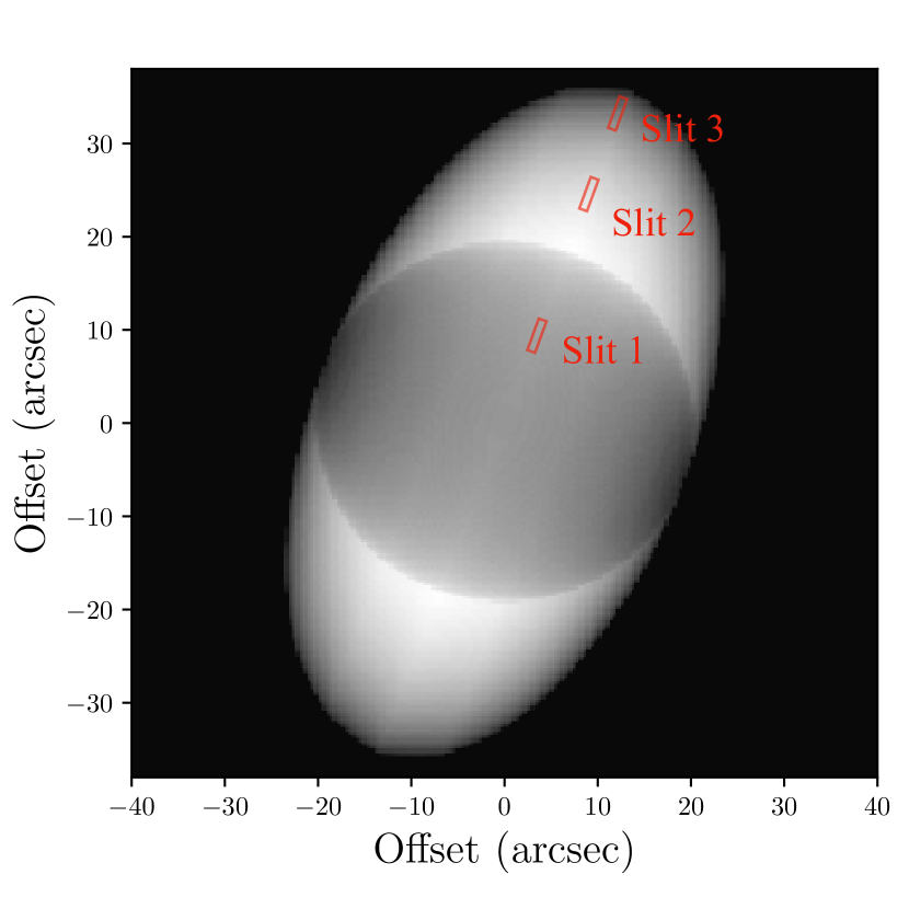
Figure 6: Density distribution of

our pyCloudy 3D model. The rectangular regions show the relative position and apertures of the pseudo-slit for the representative regions A2, A3 and A4 in NGC 6905. See results in Table 9.

Table 9: Emission line fluxes for three representative regions (A2, A3 and A4) in NGC 6905 (see Fig. 1, left), compared to the predictions for Slit1 and Slit 2 from our Cloudy models (see Fig. 6). The line fluxes are normalized with respect to H$\beta$=100.

Line	$\lambda$	From observations				Model A			Model B
	$($Å$)$	A1	A2	A3	A4	Slit 1	Slit 2	Slit 3	Slit 1	Slit 2	Slit 3
[O ii]	3727	222$\pm$12	…	21.1$\pm$1.1	18.8$\pm$3.9	164.8	198.6	383.7	142.5	159.3	200
[Ne iii]	3869	108$\pm$6	113$\pm$6	94.3$\pm$4.7	90.0$\pm$6.0	123.6	115.4	108.5	150.7	143.0	132
[Ne iii]	3968	45.6$\pm$2.3	46.3$\pm$2.3	42.9$\pm$4.9	40.1$\pm$2.5	37.5	35.0	32.9	45.7	43.4	40.1
H$\delta$	4102	25.7$\pm$1.3	25.0$\pm$10.1	24.8$\pm$1.6	25.3$\pm$1.4	26.2	26.2	26.2	26.2	26.2	26.2
H$\gamma$	4341	46.2$\pm$3.6	47.6$\pm$3.3	45.8$\pm$2.3	45.8$\pm$2.3	47.5	47.4	47.5	47.7	47.5	47.5
[O iii]	4363	13.8$\pm$2.1	14.4$\pm$1.9	12.4$\pm$0.7	11.0$\pm$0.6	15.2	13.3	10.9	22.3	20.5	17.6
He i	4471	2.7$\pm$1.5	…	1.0$\pm$0.2	1.2$\pm$0.2	2.8	3.2	3.9	2.0	2.2	2.8
[Ar iv]	4711	…	4.8$\pm$1.3	5.4$\pm$0.3	5.8$\pm$0.3	5.4	3.4	1.3	11.3	8.1	4.7
[Ar iv]	4740	…	…	4.1$\pm$0.3	4.3$\pm$0.3	3.9	2.5	1.0	8.2	5.8	3.4
[O iii]	4959	347$\pm$18	385$\pm$120	353$\pm$18	310$\pm$16	419	398	347	509	504	480
[O iii]	5007	1037$\pm$56	1169$\pm$62	1049$\pm$53	926$\pm$47	1250	1188	1034	1518	1503	1430
[Cl iii]	5518	1.5$\pm$0.9	…	0.9$\pm$0.1	0.7$\pm$0.1	1.8	1.8	1.9	2.0	2.1	2.1
[Cl iii]	5538	1.1$\pm$0.9	…	0.6$\pm$0.1	0.6$\pm$0.1	1.5	1.5	1.5	1.6	1.6	1.6
[N ii]	5755	3.9$\pm$0.9	…	0.2$\pm$0.1	…	0.2	0.3	0.7	0.2	0.2	0.4
He i	5876	9.9$\pm$1.1	6.2$\pm$1.4	3.7$\pm$0.2	3.6$\pm$0.2	8.4	9.4	11.4	6.1	6.7	8.3
[N ii]	6548	60.6$\pm$3.1	7.1$\pm$1.2	3.4$\pm$0.2	2.7$\pm$0.2	3.8	4.2	10.7	1.9	2.1	4.8
H$\alpha$	6563	283$\pm$15	285$\pm$15	260$\pm$13	271$\pm$14	276	275	276	277	276	276
[N ii]	6584	187$\pm$10	21.9$\pm$1.5	9.8$\pm$0.5	7.8$\pm$0.4	11.2	12.6	31.4	5.6	6.3	14.1
He i	6678	1.7$\pm$0.9	1.7$\pm$1.1	1.4$\pm$0.1	1.4$\pm$0.1	2.0	2.2	2.8	1.4	1.6	2.0
[S ii]	6716	17.4$\pm$1.2	5.4$\pm$1.1	2.7$\pm$0.2	2.2$\pm$0.1	2.9	3.3	6.3	2.1	2.4	4.4
[S ii]	6731	15.5$\pm$1.1	4.2$\pm$1.1	2.4$\pm$0.2	2.0$\pm$0.1	3.0	3.4	6.4	2.0	2.2	4.1
He i	7065	2.4$\pm$1.6	…	…	0.5$\pm$0.2	2.0	2.1	2.7	1.4	1.5	1.9

Taking advantage of our high-quality optical spectra of NGC 6905, which were used to study the physical properties and abundances of this PNe, in addition to the available IR and radio observations, we can test the predictions from our stellar atmosphere PoWR model using the photoionization code Cloudy (version 17.01; Ferland et al., 2017). Cloudy calculates the emissivity of the gas taking into account the dust present in the nebula. Furthermore, using the pyCloudy routines (Morisset, 2013) we can produce synthetic optical and IR observations from pseudo 3D models which can be directly compared to the observations presented here.

In order to create a 3D model of NGC 6905, ten 1D models were generated by varying the external radius of each of them as a function of the latitudinal angle $\theta$ with respect to the equatorial plane (from 0^∘ to 90^∘ with steps of 10 degrees). Subsequently, pyCloudy re-computes the 1D models and builds the pseudo 3D model. A detailed description of this process can be found in Gesicki, Zijlstra, & Morisset (2016).

Cloudy requires as an input: the source of ionization (spectral shape and $L_{\star}$), the density distribution of the nebula (geometry, density and chemical abundances) and the dust properties (size distribution and composition). For this, we used the NLTE stellar atmosphere PoWR model of HD 193949 discussed in Section 3.2 as the ionizing source. The morphology has been defined as an ellipsoidal shape with a spherical cavity as suggested by the NOT and Spitzer IRAC images (see also Phillips & Ramos-Larios, 2010). A semi-minor axis of 7.5$\times$10¹⁷ cm and a semi-major axis of 1.5$\times$10¹⁸ cm. Two cases for the density have been selected, Model A with $n_{\mathrm{e}}$=600 cm^-3 and Model B with $n_{\mathrm{e}}$=400 cm^-3, which are the limiting density values of the $n_{\mathrm{e}}$([S ii]) listed in Table 8. Figure 6 shows the density distribution of the pyCloudy 3D model. The rectangular regions in this figure labeled as S1, S2 and S3 show the relative position and apertures of the synthetic pseudo-slits which are representative of regions A1, A2, A3 and A4 defined in Figure 1.

To achieve a good fit to the emission lines, we had to tailor some of the elemental abundances. We started our model by adopting averaged abundance values obtained for A1–A4 and A6–A8 listed in the bottom rows of Table 8. However, some of these were varied in order to produce a good fit to the emission lines. Figure 7 compares the abundances used in our best Cloudy models in comparison with the averaged abundances from different elements. In all cases, the elemental abundances were slightly varied but still within the error bars of the averaged values.

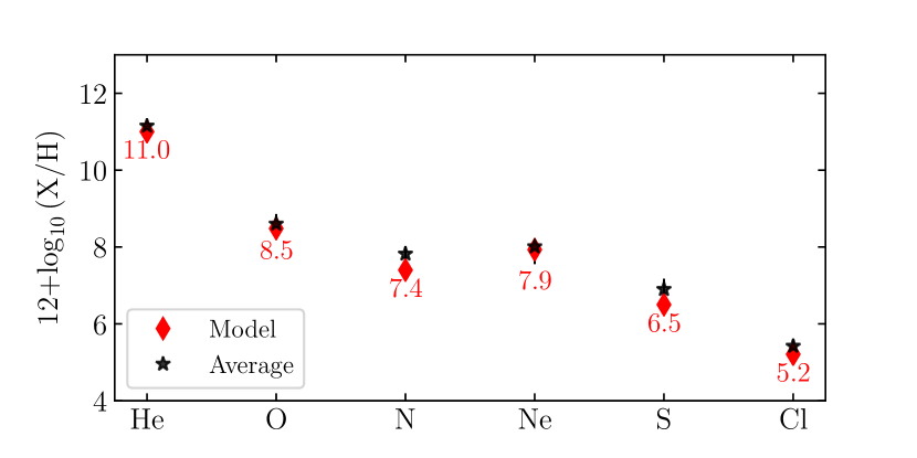
Figure 7: Elemental abundances of NGC 6905. Red diamonds shows the values used as Cloudy input while black star is the averaged value in all slit positions. The length of the black vertical lines correspond to the minimum and maximum value observed in the nebula.

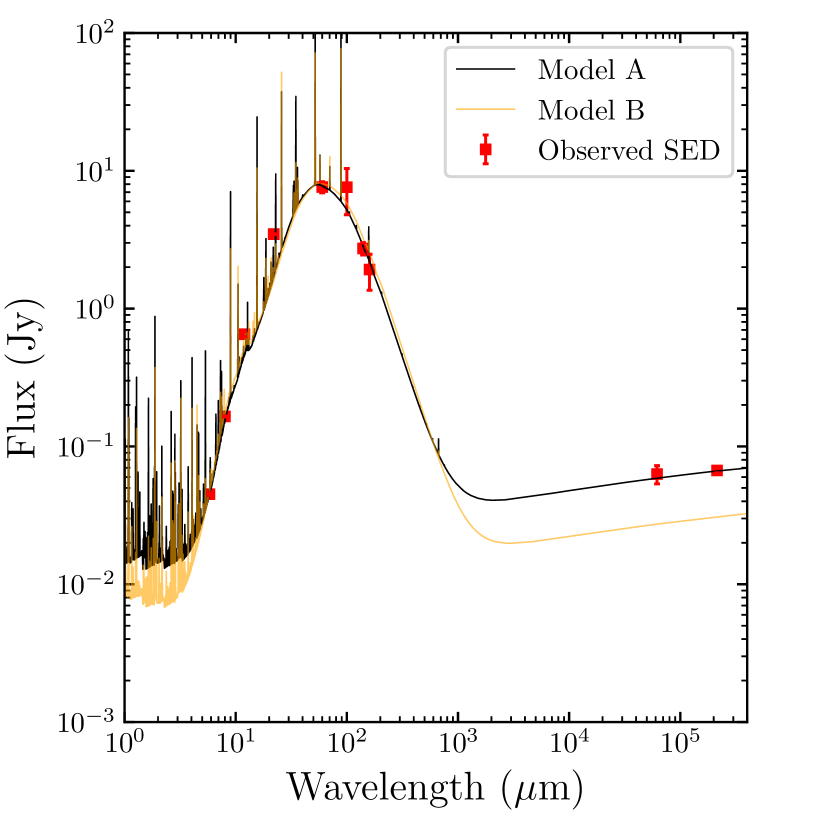
Figure 8: Observed IR photometry of NGC 6905 (red squares) compared to synthetic spectra obtained with Cloudy. Model A fits the radio measurements whilst Model B appropriately describes H$\beta$ flux.

Figure 8 presents the observed SED listed in Table 3 which includes IR and radio measurements, this peaks at $\sim$70 $\mu$m. To model the SED of NGC 6905, we included amorphous C in our Cloudy models with a power-law size distribution of $N(a)\propto a^{-3.5}$ (Mathis et al., 1977). Several combination of dust size distribution were attempted in order to produce a good fit to the SED. We found that it is necessary to include two populations of grains: a small population of dust with sizes $a_{\mathrm{small}}$=[0.001–0.002] $\mu$m and a second one with $a_{\mathrm{big}}$=[0.01–0.05] $\mu$m.

The peak of the IR emission is reproduced by the big grains while the small grains are necessary to fit the SED below 25 $\mu$m. In Figure 8 we compare the synthetic photometry from our Cloudy models to the observed SED. Both of our models fit most of the SED with a certain deviation for wavelengths between 15–30 $\mu$m. This problem was discussed by Gómez-Llanos et al. (2018) for the H-rich PN IC 418 and by Toalá et al. (2021) for the H-deficient born-again PNe A 30 and A 78. This lack of emission has been attributed to the presence of hydrogenated carbonaceous species not included in the current version of Cloudy.

Model A is able to reproduce most of the optical emission lines as well as the SED down to radio frequencies. The emission line fluxes from our model are compared to those obtained from observations in Table 9. Model A makes a good job fitting most of the emission lines, although we note that there is a large discrepancy with the [O ii] $\lambda 3727$ emission line as our model exceeds 8 times the measured values from the central slits. The flux obtained from our model is more consistent with the outer regions of NGC 6905 (slits A1 and A8). We speculate that the differences between our model and the observed emission lines might be attributed to shocks produced by the fast stellar wind of HD 193949. The CSPN of WRPNe possess strong stellar winds and have bee reported to exhibit the highest expansion velocities compared to PN harboring H-rich CSPN (see Peña et al., 2003).

The synthetic optical emission lines were used to estimate $T_{\mathrm{e}}$([O iii]), $T_{\mathrm{e}}$([N ii]) and $n_{\mathrm{e}}$([S ii]), which are also consistent with those estimated from observations (see top rows of Table 10). Finally, the estimated ionized mass of this model is 0.464 M_⊙ with a mass of dust of $\sim 1.7\times 10^{-3}$ M_⊙, for an averaged dust-to-gas ratio of 0.36 per cent by mass. A total mass of $M_{\mathrm{TOT}}$= $M_{\mathrm{gas}}+M_{\mathrm{dust}}$=0.466 M_⊙ results from this model. Details are listed in Table 10.

Table 10: Cloudy model results.

Parameter	Model A			Model B
	Slit 1	Slit 2	Slit 3	Slit 1	Slit 2	Slit 3
$T_{\mathrm{e}}$ ([O iii]) [K]	12700	11970	11685	13300	12900	12400
$T_{\mathrm{e}}$ ([N ii]) [K]	12300	11860	11734	12780	12700	12460
$n_{\mathrm{e}}$ ([S ii]) [cm-3]	510	487	486	720	710	700
log(H$\beta$) [erg cm-2 s-1]	$-$12.53	$-$12.40	$-$13.00	$-$12.90	$-$12.76	$-$13.39
$M_{\mathrm{TOTAL}}$ [M⊙]	4.66$\times 10^{-1}$			3.10$\times 10^{-1}$
$M_{\mathrm{Gas}}$ [M⊙]	4.64$\times 10^{-1}$			3.07$\times 10^{-1}$
$M_{\mathrm{Dust}}$ [M⊙]	1.69$\times 10^{-3}$			2.24$\times 10^{-3}$
$a_{\mathrm{big}}$ [M⊙]	1.46$\times 10^{-3}$			1.94$\times 10^{-3}$
$a_{\mathrm{small}}$ [M⊙]	2.25$\times 10^{-4}$			2.98$\times 10^{-4}$

One of the major difficulties of Model A was to simultaneously fit the H$\beta$ and the radio photometry. Both spectral features are directly related to the ionized mass of the model and there was a certain degeneracy between models. For this, Model A was produced so that we can give priority to the radio measurements. This resulted in a H$\beta$ flux $\sim$2 times larger than the observed. For this, we used Model B to try to fit the H$\beta$ flux. Model B is also compared to the observed SED in Figure 8 with a yellow solid line. The intensity of the synthetic emission lines of Model B are also listed in Table 9 and the global properties of the model are listed in Table 10.

The differences between Model A and B are evident in the SED. Model B cannot reproduce the radio measurements (see Fig. 8). However, the prediction for the H$\beta$ line flux are consistent with those extracted from regions A1–A4 (see Table 7). Model A resulted in a $M_{\mathrm{TOT}}$ 50 per cent larger than that of Model B. Furthermore, although Model B produces slightly larger $T_{\mathrm{e}}$ than Model A, these are still consistent with values obtained from observations.

We conclude that a more accurate model might be achieved by further including clumps and filaments within NGC 6905, but such an elegant model is out of the scope of the present paper.

4 DISCUSSION

The NOT ALFOSC spectrum of HD 193949 presented here has an unprecedented quality compared to previous studies of this [WR]-type CSPN (see Peña et al., 1998; Acker & Neiner, 2003). We have been able to identify the three classic WR features (VB, BB and the RB) plus other 21 broad features also originating from the WR star. The presence of so many lines makes it complex to assign a spectral type under the currently accepted classification schemes (e.g., Crowther et al., 1998; Acker & Neiner, 2003), but we note that the emission line ratios described in Section 3.1 suggests that HD 193949 can be classified as a [WR]-type star of the oxygen sequence no later than [WO2].

In addition, we have detected the broad emission lines of Ne vii at 4555 Å and 5666 Å, and Ne viii at 6068 Å. It has been demonstrated by Werner et al. (2007) that these features, initially attributed to O vii and O viii, can be reproduced by model atmospheres containing Ne vii and Ne viii. However, our stellar atmosphere modelling performed with the PoWR code confirms previous suggestions that HD 193949 is a [WO]-type star with a temperature of $\sim$140 kK that could not provide such highly ionized O species. Furthermore, we identified the Ne viii at 1163 and 1165 Å  in the FUSE observations presented in Fig. 4.

One cannot avoid to mention that the sub-classification schemes proposed for [WO]-type stars (Crowther et al., 1998; Acker & Neiner, 2003) are based on the alleged presence of the O vii and O viii lines. Considering this, the classification scheme needs to be updated for one that is based on high-resolution spectra that could include the comparison of more broad spectral lines including Ne lines of high ionization potential. Furthermore, this would also have an impact on the construction of new theoretical models for WRPNe.

The high signal-to-noise of the ALFOSC spectrum allowed us to extract spectra from different regions in NGC 6905: two corresponding to the low-ionization knots located at the farthermost NW and SE regions (A1 and A8) of this PN plus 5 inner regions (A2, A3, A4, A6 and A7). As expected, the A1 and A8 spectra exhibit the presence of low-ionization species such as [N i] and [O i] lines. On the other hand, the high-ionization [Ar v] ion is only detected in the innermost regions (A3, A4 and A6). The physical parameter analysis seems to suggest that NGC 6905 has more or less constant $T_{\mathrm{e}}$ and $n_{\mathrm{e}}$ along the slit of the ALFOCS spectrograph.

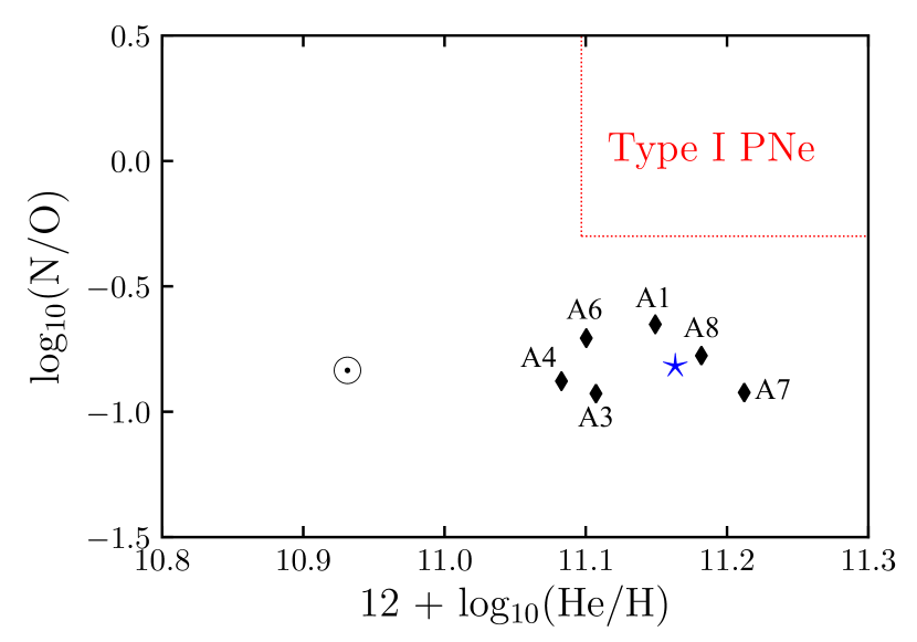
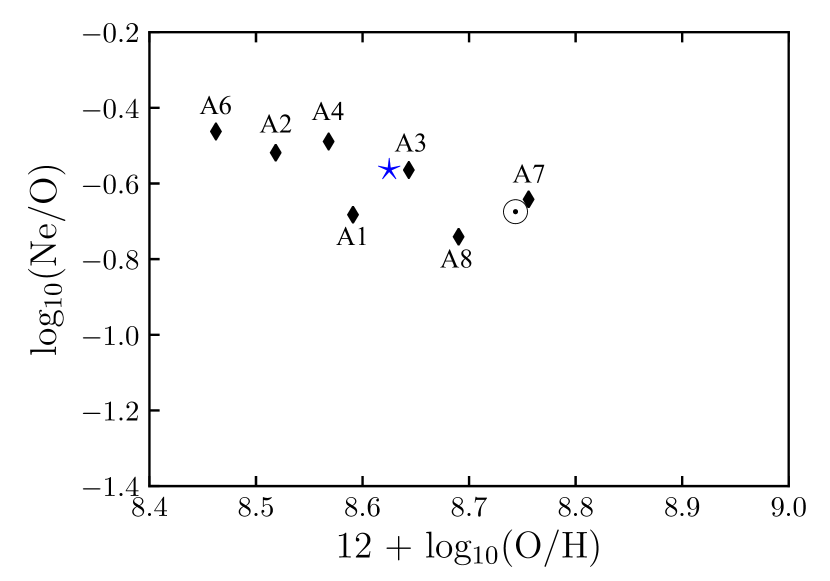
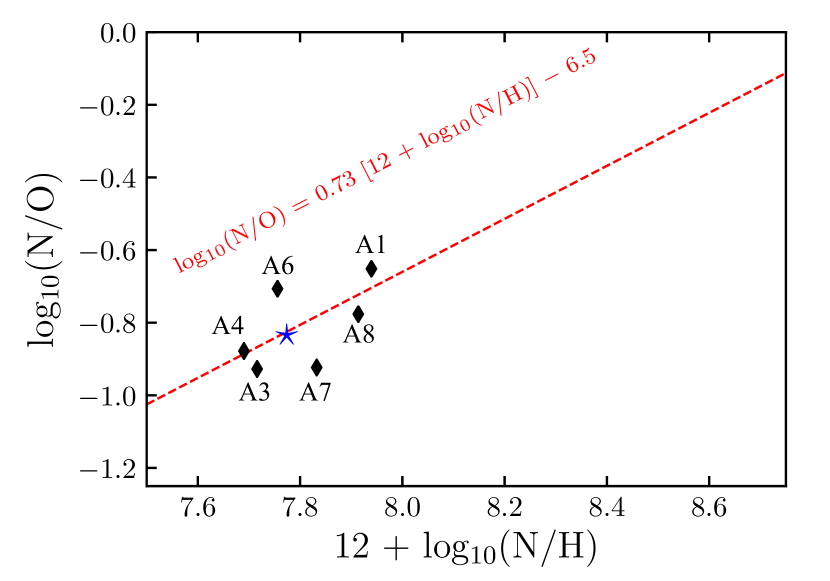
Figure 9: Abundance ratio determinations of different elements obtained from values listed in Table 8. Diamonds represent values from slits A1–A8. The panels show the averaged value using all these slits in NGC 6905 with a blue star. The solar values from Lodders (2010) are also illustrated. The top panel shows the N/O ratio versus the He abundance. Here the region for the Type I PNe defined by Peimbert (1990) is shown with red dotted-lines. The middle panel displays the Ne/O ratio versus the O abundance. The bottom panel presents the N/O ratio versus the N abundance. The red dashed-line corresponds to the relation presented in García-Rojas et al. (2013) (see Eq. (4) and details in the text).

Furthermore, there is not a large difference between the total abundance determinations among the inner regions and the low-ionization knots. To facilitate a comparison, we have created the abundance ratio diagrams presented in Figure 9. In the top panel we compare the N/O ratio versus the He abundance and in the middle panel we compare the Ne/O ratio versus the O abundance. Averaged values are shown with a blue star on each panel. None of the different regions within NGC 6905 stands with different abundances. In fact, the averaged abundances are consistent with other WRPNe analysed in García-Rojas et al. (2013). Fig. 9 shows that our N/O values are located at the lower limits found by these authors, whilst the Ne/O ratio is within the reported values (see figures 6 and 9 in García-Rojas et al., 2013).

According to the Peimbert classification (Peimbert, 1990; Peimbert et al., 2017), Type I PNe have ages $\sim$1 Gyr and initial masses $>$2 M_⊙, Type II: $\sim$1–5 Gyr and $\sim$1.2–2 M_⊙, Type III: $\sim$5 Gyr and $\sim$1.2 M_⊙ and Type IV: $>$5 Gyr and $<$1 M_⊙, in addition to being located in the Galactic halo. Opposite to Type II and III PNe, Type I PNe present He- and N-rich envelopes (He/H$>$0.125 and N/O$>$0.5). Following García-Rojas et al. (2013), the region of the Type I PNe is shown in Figure 9 (top panel) as a reference. Our object is clearly far from that region. Just for completeness, the Galactic latitude of NGC 6905 corresponds to values within the disk of the Galaxy ($l$, $b$ [deg] = 61.491253, $-$9.571280). Thus, a Type IV classification is clearly ruled out.

We conclude that there is no anomalous C-enrichment within NGC 6905 which suggests that no very late thermal pulse (VLTP) has been involved in the formation of this PNe or the production of its [WR] CSPN. This is further corroborated by the very low N abundance of the stellar wind , $<10^{-4}$ by mass, compared to what is expected from models accounting for the VLTP scenario of $\sim$0.1 by mass (e.g. Herwig, 2001; Althaus et al., 2005).

Interestingly, the averaged values of 12$+$log₁₀(N/H)=7.75 and log₁₀(N/O)=$-$0.863 obtained for NGC 6905 follow the relation described in García-Rojas et al. (2013):

$$\mathrm{log_{10}(N/O)}=0.73\left[12+\mathrm{log_{10}(N/H)}\right]-6.5,$$ (4)

with a difference of only $\approx$0.02 dex. We illustrate this in the bottom panel of Figure 9. García-Rojas et al. (2013) obtained Eq. (4) by fitting their observations. These authors argue that this relation follows from the fact that N enrichment occurs independently of the O abundance in PNe, implying that this is at the expense of C. Unfortunately, we are not able to estimate the C abundance to study this effect. García-Rojas et al. (2013) compare Eq. (4) with predictions from stellar evolution models presented by Karakas (2010) in their figure 6 (lower panel). According to that figure, NGC 6905 is placed at the lower left region of the diagram, suggesting that the progenitor mass of the CSPN of NGC 6905 had an initial mass of $\sim$1 M_⊙.

With the synthetic SED obtained with our PoWR model we were able to calculate a Cloudy model for NGC 6905 that reproduces quite well the observed nebular and dust properties. We would like to remark that detailed models of the nebular and dust properties of PNe using a family of dust populations have been recently presented in the literature. In particular, we remark the work of Gómez-Llanos et al. (2018). These authors included in their photoionization Cloudy models graphite, amorphous C, SiC and MgS to reproduce all the spectral features in the PN IC 418. Such detailed analysis is out of the scope of this paper and only amorphous C is used in our Cloudy model which is then used to estimate the total mass of gas and dust. However, we note that including more dust species in the model, will not change dramatically the nebular properties and estimated masses.

Our Cloudy models suggest a total mass for NGC 6905 in the range of 0.31 M_⊙ and 0.47 M_⊙ with a dust mass of $\approx 2\times 10^{-3}$ M_⊙, that is, a dust-to-gas ratio of 0.43–0.65 per cent. Adopting a current mass of 0.6 M_⊙ for HD 193949 this amounts to an upper limit for the total mass of $\sim$1.07 M_⊙. Interestingly, our photoionization model is consistent with predictions from the N/O ratio versus N abundance. This suggests that most of the mass previously lost by the star is still in its vicinity and its currently photoionized by the strong UV flux from the CS. This seems to suggest that NGC 6905 is one of the WRPN with the less massive progenitor star.

Finally, NGC 6905 is included in the catalogue of new candidate binaries of Chornay et al. (2021, see their table A.1), however, until there are comprehensive photometric follow-ups, the conclusive evidence of its probable binary nature is still lacking. Recently Jacoby et al. (2021) reported the identification of binary CSPNe with Kepler/K2 observations. NGC 6905 is not included, however, given the richness of observations such as those of TESS, more studies regarding the binarity issue for this and other CSPNe are to be expected.

5 SUMMARY AND CONCLUDING REMARKS

We presented a multi-wavelength characterisation of the PN NGC 6905 which harbours the [WR] CSPN HD 193949. We combined UV, optical, IR and radio observations to fully characterise the physical properties of this WRPN NGC 6905. Our findings can be summarized as follows:

• The high-quality NOT ALFOSC spectrum of HD 193949 allowed us to detect the three broad WR bumps, the so-called VB, BB and RB, confirming that this CSPN belongs to the [WO]-class of [WR] stars. Along with these classic broad features we also detected 21 WR features that include He ii, C iv, O v and O vi which suggest that the spectral type of HD 193949 cannot be later than a [WO2]-subtype star.

• Additionally to the two tens of WR features, we also detected broad emission features at $\lambda$4555, $\lambda$5666 and $\lambda$6068 Å, previously identified as emission lines from O vii and O viii, which according to more recent studies might be actually originated from stellar Ne vii and Ne viii. HD 193949 is yet another CSPN with an effective temperature of $\sim$140 kK that could not provide such high ionization O species. We confirm the presence of the Ne lines in the FUSE spectrum of HD 193949. We suggest that an updated classification scheme is needed, one that may also accounts for the Ne emission lines.

• We determined the main physical properties of the [WR] CSPN by using state-of-the-art non-LTE PoWR models. We analysed the optical spectrum and found that a model with $T_{\mathrm{eff}}$= $140$ kK and surface-abundance pattern of H/He/C/N/O/Ne/Fe= $<$0.05/0.55/0.35/$<$0.000069/0.08/0.02/0.0014 (by mass) reproduces the observations sufficiently well. We confirm the high terminal velocity of the stellar wind of $\text{v}_{\infty}=2000\pm 100~{}$km s^-1.

• We studied the physical properties of different regions of NGC 6905. We found that the low-ionization knots located at the NW and SE regions of NGC 6905 do not exhibit different $n_{\mathrm{e}}$ nor $T_{\mathrm{e}}$ compared to the inner regions in this WRPN. We estimated averaged values of $n_{\mathrm{e}}$([S ii]) = 500 cm^-3 with $T_{\mathrm{e}}$ ranging around 13 kK.

• The total abundances obtained from different regions within NGC 6905 resulted in very similar values, which means that the low-density knots were not produced as part of a VLTP. NGC 6905 has similar abundances as other WRPN, but slightly smaller N/O ratio. In particular, comparing the N/O ratio versus the N abundance following previous studies suggests that the CSPN of NGC 6905 had a relatively low initial mass of $\sim$1 M_⊙. This makes NGC 6905 one of the WRPN with the less massive central star. We conclude that the underabundance of N in the stellar wind, the lack of C-enrichment in the PN and its chemically homogenous structure imply that NGC 6905 is not the result of a VLTP.

• Finally, we used Cloudy to produce a photoionization model of NGC 6905 with the stellar atmosphere model obtained with PoWR for HD 193949 as the ionization source and the abundances determined in this paper. Amorphous C is included in the calculations. Our model simultaneously reproduces the nebular and dust properties of NGC 6905 and suggests that the total mass of gas of NGC 6905 is in the range of 0.31 M_⊙ and 0.47 M_⊙ with a mass of dust of around $2.24\times 10^{-3}$ M_⊙ and $1.69\times 10^{-3}$ M_⊙ respectively. That is, a dust-to-gas ratio less than 0.7 per cent. Adopting a current mass of 0.6 M_⊙ for HD 193949, we estimate that its initial mass was around 1.07 M_⊙, very similar to that estimated by comparing abundances with stellar evolution models.

Data availability

The data underlying this work will be shared on reasonable request to the first author.

References

- Acker & Neiner (2003) Acker, A., & Neiner, C. 2003, A&A, 403, 659
- Acker et al. (1996) Acker, A., Górny, S. K., & Stenholm, B. 1996, Ap&SS, 238, 63
- Althaus et al. (2005) Althaus, L. G., Serenelli, A. M., Panei, J. A., et al. 2005, A&A, 435, 631-648
- Bailer-Jones et al. (2021) Bailer-Jones, C. A. L., Rybizki, J., Fouesneau, M., Demleitner, M., & Andrae, R. 2021, AJ, 161, 147
- Cardelli et al. (1989) Cardelli, J. A. A., Clayton, G. C., Mathis, J. S. 1989, ApJ, 345, 245
- Crowther et al. (1998) Crowther, P. A., De Marco, O., & Barlow, M. J. 1998, MNRAS, 296, 367
- Crowther (2007) Crowther, P. A. 2007, ARA&A, 45, 177
- Cuesta et al. (1993) Cuesta, L., Phillips, J. P., & Mampaso, A. 1993, A&A, 267, 199
- Chornay et al. (2021) Chornay, N., Walton, N. A., Jones, D., et al. 2021, arXiv:2101.01800
- Delgado-Inglada et al. (2014) Delgado-Inglada G., Morisset C., Stasińska G., 2014, MNRAS, 440, 536
- Ferland et al. (2017) Ferland, G. J., et al. 2017, Rev. Mex. Astron. Astrofis., 53, 385-438
- Ferrarotti & Gail (2006) Ferrarotti, A. S. & Gail, H.-P. 2006, A&A, 447, 553
- Frank et al. (2018) Frank, A., et al. 2018, Galaxies, 6, 113
- Gaia Collaboration et al. (2020) Gaia Collaboration et al. 2020, arXiv:2012.01533
- García-Rojas et al. (2013) García-Rojas et al. 2013, A&A, 558, A122
- Gesicki et al. (2003) Gesicki, K. et al. 2003, A&A, 400, 957
- Gesicki, Zijlstra, & Morisset (2016) Gesicki K., Zijlstra A. A., Morisset C., 2016, A&A, 585, A69
- Gómez-González et al. (2020) Gómez-González, V. M. A. et al. 2020, MNRAS, 496, 959
- Gómez-González et al. (2020) Gómez-González, V. M. A. et al. 2020, MNRAS, 493, 3879-3892
- Gómez-Llanos et al. (2018) Gómez-Llanos, V., Morisset, C., Szczerba, R., et al. 2018, A&A, 617, A85
- Górny & Tylenda (2000) Górny, S. K. & Tylenda, R. 2000, A&A, 362, 1008
- Gräfener et al. (2002) Gräfener, G., Koesterke, L., & Hamann, W.-R. 2002, A&A, 387, 244
- Guerrero et al. (2020) Guerrero, M. A. et al. 2020, MNRAS, 495, 2234
- Guerrero & De Marco (2013) Guerrero, M. A. & De Marco, O. 2013, A&A, 553, A126
- Hajduk et al. (2018) Hajduk, M. et al. 2018, MNRAS, 479, 5657
- Hamann & Gräfener (2004) Hamann, W.-R., & Gräfener, G. 2004, A&A, 427, 697
- Herald & Bianchi (2011) Herald, J. E. & Bianchi, L. 2011, MNRAS, 417, 2440
- Herwig (2001) Herwig, F. 2001, Ap&SS, 275, 15-26
- Iaconi et al. (2017) Iaconi, R. et al. 2017, MNRAS, 464, 4028
- Jacoby et al. (2021) Jacoby, G. H., Hillwig, T. C., Jones, D., et al. 2021, arXiv:2104.07934
- Jiménez-Hernández et al. (2021) Jiménez-Hernández, P., Arthur, S. J., Toalá, J. A., et al. 2021, arXiv:2108.03321
- Jiménez-Hernández et al. (2020) Jiménez-Hernández, P., Arthur, S. J. and Toalá, J. A., 2020, MNRAS, 497, 4128-4142
- Karakas (2010) Karakas, A. I. 2010, MNRAS, 403, 1413
- Keller et al. (2014) Keller, G. R., Bianchi, L., & Maciel, W. J. 2014, MNRAS, 442, 1379
- Keller et al. (2011) Keller, G. R. et al. 2011, MNRAS, 418, 705
- Kepler et al. (2016) Kepler, S. O., Pelisoli, I., Koester, D., et al. 2016, MNRAS, 455, 3413
- Kingsburgh & Barlow (1994) Kingsburgh, R. L. & Barlow, M. J. 1994, MNRAS, 271, 257
- Kwok (2000) Kwok, S. 2000, The origin and evolution of planetary nebulae / Sun Kwok. Cambridge ; New York : Cambridge University Press, 2000. (Cambridge astrophysics series ; 33)
- Lau et al. (2011) Lau, H. H. B., De Marco, O., & Liu, X.-W. 2011, MNRAS, 410, 1870
- Lodders (2010) Lodders, K. 2010, Astrophysics and Space Science Proceedings, 16, 379
- Luridiana et al. (2015) Luridiana, V., Morisset, C., & Shaw, R. A. 2015, A&A, 573, A42
- Marcolino et al. (2007) Marcolino, W. L. F. et al. 2007, ApJ, 654, 1068-1086
- Mathis et al. (1977) Mathis, J. S., Rumpl, W., Nordsieck, K. H. 1977, ApJ, 217, 425-433
- Mauron et al. (2013) Mauron, N., Huggins, P. J., & Cheung, C.-L. 2013, A&A, 551, A110
- Medina et al. (2006) Medina, S. et al. 2006, Rev. Mex. Astron. Astrofis., 42, 53
- Miller Bertolami (2016) Miller Bertolami, M. M. 2016, A&A, 588, A25
- Miszsalski et al. (2012) Miszalski, B., Crowther, P. A., De Marco, O. et al. 2012, MNRAS, 423, 934-947
- Morisset (2013) Morisset, C. 2013, Astrophysics Source Code Library, record ascl:1304.020
- Osterbrock & Ferland (2006) Osterbrock, D. E., & Ferland, G. J. 2006, Astrophysics of gaseous nebulae and active galactic nuclei
- Peimbert (1990) Peimbert, M. 1990, Reports on Progress in Physics, 53, 1559
- Peimbert et al. (2017) Peimbert, M., Peimbert, A. & Delgado-Inglada, G. 2017, PASP, 129, 082001
- Peña et al. (2003) Peña, M., Medina, S., & Stasińska, G. 2003, Revista Mexicana de Astronomia y Astrofisica Conference Series, 15, 38
- Peña et al. (2001) Peña, M., Stasińska, G., & Medina, S. 2001, A&A, 367, 983
- Peña et al. (1998) Peña, M., Stasińska, G., Esteban, C., et al. 1998, A&A, 337, 866
- Phillips & Ramos-Larios (2010) Phillips, J. P. & Ramos-Larios, G. 2010, MNRAS, 405, 2179
- Press et al. (1992) Press, W. H. et al. 1992, Numerical recipes in FORTRAN. The Art of Scientific Computing. Cambridge Univ. Press, Cambridge
- Rechy-García et al. (2017) Rechy-García, J. S. et al. 2017, MNRAS, 464, 2318
- Rubio et al. (2020) Rubio, G. et al. 2020, MNRAS, 499, 415-427
- Sabbadin & Hamzaoglu (1982) Sabbadin, F. & Hamzaoglu, E. 1982, A&AS, 50, 1
- Schmutz et al. (1989) Schmutz, W., Hamann, W.-R., & Wessolowski, U. 1989, A&A, 210, 23
- Toalá et al. (2021) Toalá, J. A., Jiménez-Hernández, P., Rodríguez-González, J. B., et al. 2021, MNRAS
- Toalá et al. (2020) Toalá, J. A. et al. 2020, MNRAS, 494, 3784
- Todt et al. (2006) Todt, H., Gräfener, G., & Hamann, W.-R. 2006, in Planetary Nebulae in our Galaxy and Beyond, ed. M. J. Barlow & R. H. Méndez, Vol. 234, 127–130
- Todt et al. (2008) Todt, H., Hamann, W.-R., & Gräfener, G. 2008, in Clumping in Hot-Star Winds, ed. W.-R. Hamann, A. Feldmeier, & L. M. Oskinova, 251
- Todt et al. (2010) Todt, H. et al. 2010, A&A, 515, A83
- Todt et al. (2013) Todt, H. et al. 2013, MNRAS, 430, 2302
- Todt et al. (2015) Todt, H. et al. 2015, A&A, 579, A75
- Tody (1993) Tody, D. 1993, Astronomical Data Analysis Software and Systems II, 173
- Tresse et al. (1999) Tresse et al. 1999, MNRAS, 310, 262
- Vassiliadis & Wood (1993) Vassiliadis, E. & Wood, P. R. 1993, ApJ, 413, 641
- Weidmann et al. (2020) Weidmann, W. A. et al. 2020, A&A, 640, A10
- Werner et al. (2007) Werner, K., Rauch, T., & Kruk, J. W. 2007, A&A, 474, 591
- Wesson et al. (2018) Wesson, R. et al. 2018, MNRAS, 480, 4589