Path Regularization: A Convexity and Sparsity Inducing Regularization for Parallel ReLU Networks

Abstract

Understanding the fundamental principles behind the success of deep neural networks is one of the most important open questions in the current literature. To this end, we study the training problem of deep neural networks and introduce an analytic approach to unveil hidden convexity in the optimization landscape. We consider a deep parallel ReLU network architecture, which also includes standard deep networks and ResNets as its special cases. We then show that pathwise regularized training problems can be represented as an exact convex optimization problem. We further prove that the equivalent convex problem is regularized via a group sparsity inducing norm. Thus, a path regularized parallel ReLU network can be viewed as a parsimonious convex model in high dimensions. More importantly, since the original training problem may not be trainable in polynomial-time, we propose an approximate algorithm with a fully polynomial-time complexity in all data dimensions. Then, we prove strong global optimality guarantees for this algorithm. We also provide experiments corroborating our theory.

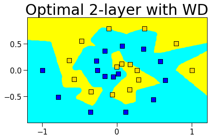
(a) 2-layer NN with WD

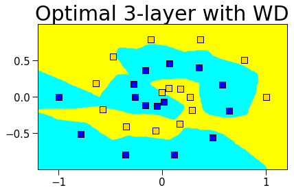
(b) 3-layer NN with WD

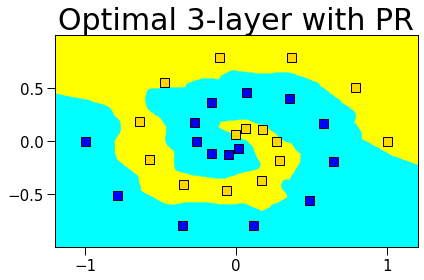
(c) 3-layer NN with PR (Ours)

Figure 1: Decision boundaries of 2-layer and 3-layer ReLU networks that are globally optimized with weight decay (WD) and path regularization (PR). Here, our convex training approach in (c) successfully learns the underlying spiral pattern for each class while the previously studied convex models in (a) and (b) fail (see Appendix A.1 for details).

1 Introduction

Deep Neural Networks (DNNs) have achieved substantial improvements in several fields of machine learning. However, since DNNs have a highly nonlinear and non-convex structure, the fundamental principles behind their remarkable performance is still an open problem. Therefore, advances in this field largely depend on heuristic approaches. One of the most prominent techniques to boost the generalization performance of DNNs is regularizing layer weights so that the network can fit a function that performs well on unseen test data. Even though weight decay, i.e., penalizing the $\ell_{2}^{2}$-norm of the layer weights, is commonly employed as a regularization technique in practice, recently, it has been shown that $\ell_{2}$-path regularizer [1], i.e., the sum over all paths in the network of the squared product over all weights in the path, achieves further empirical gains [2]. Additionally, recent studies have elucidated that convex optimization reveals surprising generalization and interpretability properties for Deep Neural Networks (DNNs). [3, 4, 5, 6] Therefore, in this paper, we investigate the underlying mechanisms behind path regularized DNNs through the lens of convex optimization.

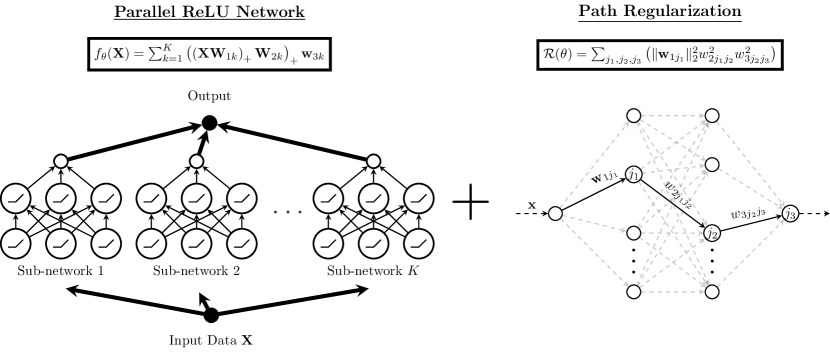
Figure 2: (Left): Parallel ReLU network in (1) with $K$ sub-networks and three layers ($L=3$) (Right): Path regularization for a three-layer network.

2 Parallel Neural Networks

Although DNNs are highly complex architectures due to the composition of multiple nonlinear functions, their parameters are often trained via simple first order gradient based algorithms, e.g., Gradient Descent (GD) and variants. However, since such algorithms only rely on local gradient of the objective function, they may fail to globally optimize the objective in certain cases [7, 8]. Similarly, [9, 10] showed that these pathological cases also apply to stochastic algorithms such as Stochastic GD (SGD). They further show that some of these issues can be avoided by increasing the number of trainable parameters, i.e., operating in an overparameterized regime. However, [11] reported the existence of more complicated cases, where SGD/GD usually fails. Therefore, training DNNs to global optimality remains a challenging optimization problem [12, 13, 14].

To circumvent difficulties in training, recent studies focused on models that benefit from overparameterization [15, 16, 17, 18]. As an example, [19, 20, 21, 22, 23] considered a new architecture by combining multiple standard NNs, termed as sub-networks, in parallel. Evidences in [20, 21, 22, 23, 24, 25] showed that this way of combining NNs yields an optimization landscape that has fewer local minima and/or saddle points so that SGD/GD generally converges to a global minimum. Therefore, many recently proposed NN-based architectures that achieve state-of-the-art performance in practice, e.g., SqueezeNet [26], Inception [27], Xception [28], and ResNext [29], are in this form.

Table 1: Complexity comparison with prior works ($n$: $\#$ of data samples, $d$: feature dimension, $m_{l}$: $\#$ of hidden neurons in layer $l$, $\epsilon$: approximation accuracy, $r$: rank of the data, $\kappa\ll r$: chosen according to (10) such that $\epsilon$ accuracy is achieved)

	Loss function	2-layer complexity	$L$-layer complexity	Globally optimal
[30]	Convex loss	$\mathcal{O}\left(2^{m_{1}}n^{dm_{1}}poly(n,d,m_{1})\right)$	-	✓(Brute-force)
[31]	$\ell_{2}$-loss	$2^{\mathcal{O}(\frac{m_{1}^{5}}{\epsilon^{2}})}poly(n,d)$	-	✗(NP-hard)
[32]	$\ell_{p}$-loss	$\mathcal{O}\left(2^{m_{1}}n^{dm_{1}}poly(n,d,m_{1})\right)$	-	✓(Brute-force)
[6]	Convex loss	$\mathcal{O}(n^{r}poly(d,r))$	-	✓(Convex, exact)
Ours	Convex loss	$\mathcal{O}(n^{r}poly(d,r))$	$\mathcal{O}\left(n^{r\prod_{j=1}^{L-2}m_{j}}poly(d,r,\prod_{j=1}^{L-2}m_{l})\right)$	✓(Convex, exact)
Ours	Convex loss	$\mathcal{O}(n^{\kappa}poly(d,\kappa))$	$\mathcal{O}\left(n^{\kappa\prod_{j=1}^{L-2}m_{j}}poly(d,\kappa,\prod_{j=1}^{L-2}m_{l})\right)$	✓(Convex, $\epsilon$-opt)

Notation and preliminaries: Throughout the paper, we denote matrices and vectors as uppercase and lowercase bold letters, respectively. For vectors and matrices, we use subscripts to denote a certain column/element. As an example, $w_{lkj_{l-1}j_{l}}$ denotes the $j_{l-1}j_{l}^{th}$ entry of the matrix $\mathbf{W}_{lk}$. We use $\mathbf{I}_{k}$ and $\mathbf{0}$ (or $\mathbf{1}$) to denote the identity matrix of size $k\times k$ and a vector/matrix of zeros (or ones) with appropriate sizes. We use $[n]$ for the set of integers from $1$ to $n$. We use $\|\cdot\|_{2}$ and $\|\cdot\|_{F}$ to represent the Euclidean and Frobenius norms, respectively. Additionally, we denote the unit $\ell_{p}$ ball as $\mathcal{B}_{p}:=\{\mathbf{u}\in\mathbb{R}^{d}\,:\,\|\mathbf{u}\|_{p}\leq 1\}$. We also use $\mathbbm{1}[x\geq 0]$ and $\left(x\right)_{+}=\max\{x,0\}$ to denote the 0-1 valued indicator and ReLU, respectively.

In this paper, we particularly consider a parallel ReLU network with $K$ sub-networks and each sub-network is an $L$-layer ReLU network (see Figure 2) with layer weights $\mathbf{W}_{lk}\in\mathbb{R}^{m_{l-1}\times m_{l}}$, $\forall l\in[L-1]$ and $\mathbf{w}_{Lk}\in\mathbb{R}^{m_{L-1}}$, where $m_{0}=d$, $m_{L}=1$, and $m_{l}$ denotes the number of neurons in the $l^{th}$ hidden layer. Then, given a data matrix ${\bf X}\in\mathbb{R}^{n\times d}$, the output of the network is as follows

$$f_{\theta}({\bf X}):=\sum_{k=1}^{K}\left(\left({\bf X}\mathbf{W}_{1k}\right)_{+}\ldots\mathbf{W}_{(L-1)k}\right)_{+}\mathbf{w}_{Lk},$$ (1)

where we compactly denote the parameters as $\theta:=\bigcup_{k}\{\mathbf{W}_{lk}\}_{l=1}^{L}$ with the parameter space as $\Theta$ and each sub-network represents a standard deep ReLU network.

Remark 1.

Most commonly used neural networks in practice can be classified as special cases of parallel networks, e.g., standard NNs and ResNets [33] see Appendix A.2 for details.

2.1 Our Contributions

• We prove that training the path regularized parallel ReLU networks (1) is equivalent to a convex optimization problem that can be approximately solved in polynomial-time by standard convex solvers (see Table 1). Therefore, we generalize the two-layer results in [6] to multiple nonlinear layer without any strong assumptions in contrast to [21] and a much broader class of NN architectures including ResNets.

• As already observed by [6, 21], regularized deep ReLU network training problems require exponential-time complexity when the data matrix is full rank, which is unavoidable. However, in this paper, we develop an approximate training algorithm which has fully polynomial-time complexity in all data dimensions and prove global optimality guarantees in Theorem 2. To the best of our knowledge, this is the first convex optimization based and polynomial-time complexity (in data dimensions) training algorithm for ReLU networks with global approximation guarantees.

• We show that the equivalent convex problem is regularized by a group norm regularization where grouping effect is among the sub-networks. Therefore the equivalent convex formulation reveals an implicit regularization that promotes group sparsity among sub-networks and generalizes prior works on linear networks such as [34] to ReLU networks.

• We derive a closed-form mapping between the parameters of the non-convex parallel ReLU networks and its convex equivalent in Proposition 1. Therefore, instead of solving the challenging non-convex problem, one can globally solve the equivalent convex problem and then construct an optimal solution to the original non-convex network architecture via our closed-form mapping.

2.2 Overview of Our Results

Given data ${\bf X}\in\mathbb{R}^{n\times d}$ and labels $\mathbf{y}\in\mathbb{R}^{n}$, we consider the following regularized training problem

$$p_{L}^{*}:=\min_{\theta\in\Theta}\mathcal{L}\left(f_{\theta}({\bf X}),\mathbf{y}\right)+\beta\mathcal{R}(\theta)\,,$$ (2)

where $\Theta:=\{\theta\in\Theta:\mathbf{W}_{lk}\in\mathbb{R}^{m_{l-1}\times m_{l}},\forall l\in[L],\forall k\in[K]\}$ is the parameter space, $\mathcal{L}\left(\cdot,\cdot\right)$ is an arbitrary convex loss function, $\mathcal{R}(\cdot)$ represents the regularization on the network weights, and $\beta>0$ is the regularization coefficient.

For the rest of the paper, we focus on a scalar output regression/classification framework with arbitrary loss functions, e.g., squared loss, cross entropy or hinge loss. We also note that our derivations can be straightforwardly extended to vector outputs networks as proven in Appendix A.11. More importantly, we use $\ell_{2}$-path regularizer studied in [1, 2], which is defined as

$$\mathcal{R}(\theta):=\sum_{k=1}^{K}\sqrt{\sum_{j_{1},j_{2},\ldots,j_{L}}\left(\|\mathbf{w}_{1kj_{1}}\|_{2}^{2}\prod_{l=2}^{L}w_{lkj_{l-1}j_{l}}^{2}\right)},$$

where $w_{lkj_{l-1}j_{l}}$ is the $j_{l-1}j_{l}^{th}$ entry of $\mathbf{W}_{lk}$. The above regularizer sums the square of all the parameters along each possible path from input to output of each sub-network $k$ (see Figure 2) and then take the squared root of the summation. Therefore, we penalize each path in each sub-network and then group them based on the sub-network index $k$.

We now propose a scaling to show that (2) is equivalent to a group $\ell_{1}$ regularized problem.

Lemma 1.

The following problems are equivalent :

$$\min_{\theta\in\Theta}~{}\mathcal{L}\left(f_{\theta}({\bf X}),\mathbf{y}\right)+\beta\mathcal{R}(\theta)~{}=~{}\min_{{\theta\in\Theta_{s}}}~{}\mathcal{L}\left(f_{\theta}({\bf X}),\mathbf{y}\right)+\beta\sum_{k=1}^{K}\|\mathbf{w}_{Lk}\|_{2},$$

where $\mathbf{w}_{Lk}\in\mathbb{R}^{m_{L-1}}$ are the last layer weights of each sub-network $k$, and $\Theta_{s}:=\{\theta\in\Theta:\sum_{j_{1},j_{2},\ldots,j_{L-2}}\left(\|\mathbf{w}_{1kj_{1}}\|_{2}^{2}\prod_{l=2}^{L-1}w_{lkj_{l-1}j_{l}}^{2}\right)\leq 1,\forall j_{L-1},\forall k\in[K]\}$ denotes the parameter space after rescaling.

The advantage of the form in Lemma 1 is that we can derive a dual problem with respect to the output layer weights $\mathbf{w}_{Lk}$ and then characterize the optimal layer weights via optimality conditions and the prior works on $\ell_{1}$ regularization in infinite dimensional spaces [35]. Thus, we first apply the rescaling in Lemma 1 and then take the dual with respect to the output weights $\mathbf{w}_{Lk}$. To characterize the hidden layer weights, we then change the order of minimization for the hidden layer weights and the maximization for the dual parameter to get the following dual problem

$$p_{L}^{*}\geq d_{L}^{*}:=\max_{\mathbf{\mathbf{v}}}-\mathcal{L}^{*}(\mathbf{v})\quad\text{ s.t. }\max_{\theta\in\Theta_{s}}\left\|\mathbf{v}^{T}\left(\left({\bf X}\mathbf{W}_{1}\right)_{+}\ldots\mathbf{W}_{(L-1)}\right)_{+}\right\|_{2}\leq\beta,$$ (3)

where $\mathcal{L}^{*}$ is the Fenchel conjugate function of $\mathcal{L}$, which is defined as [36]

$$\mathcal{L}^{*}(\mathbf{v}):=\max_{\mathbf{z}}\mathbf{z}^{T}\mathbf{v}-\mathcal{L}\left(\mathbf{z},\mathbf{y}\right).$$

The dual problem in (3) is critical for our derivations since it provides us with an analytic perspective to characterize a set of optimal hidden layer weights for the non-convex neural network in (1). To do so, we first show that strong duality holds for the non-convex training problem in Lemma 1, i.e., $p_{L}^{*}=d_{L}^{*}$. Then, based on the exact dual problem in (3), we propose an equivalent analytic description for the optimal hidden layer weights via the KKT conditions.

We note that strong duality for two-layer ReLU networks has already been proved by previous studies [19, 21, 6, 37, 22, 38], however, this is the first work providing an exact characterization for path regularized deep ReLU networks via convex duality.

3 Parallel networks with three layers

Here, we consider a three-layer parallel network with $K$ sub-networks, which is a special case of (1) when $L=3$. Thus, we have the following training problem

$$p_{3}^{*}=\min_{\theta\in\Theta}~{}\mathcal{L}\left(f_{\theta}({\bf X}),\mathbf{y}\right)+\beta\sum_{k=1}^{K}\sqrt{\sum_{j_{1},j_{2}}\|\mathbf{w}_{1kj_{1}}\|_{2}^{2}w_{2kj_{1}j_{2}}^{2}w_{3kj_{2}}^{2}}.$$ (4)

where $\Theta\,{=}\,\{(\mathbf{W}_{1k},\mathbf{W}_{2k},\mathbf{w}_{3k}):\mathbf{W}_{1k}\in\mathbb{R}^{d\times m_{1}},\mathbf{W}_{2k}\in\mathbb{R}^{m_{1}\times m_{2}},\mathbf{w}_{3k}\in\mathbb{R}^{m_{2}}\}$. By Lemma 1,

$$p_{3}^{*}=\min_{\theta\in\Theta_{s}}\mathcal{L}\left(f_{\theta}({\bf X}),\mathbf{y}\right)+\beta\sum_{k=1}^{K}\|\mathbf{w}_{3k}\|_{2}.$$ (5)

Then, taking the dual of (5) with respect to the output layer weights $\mathbf{w}_{3k}\in\mathbb{R}^{m_{2}}$ and then changing the order of the minimization for $\{\mathbf{W}_{1k},\mathbf{W}_{2k}\}$ and the maximization for the dual variable $\mathbf{v}$ yields

$$p_{3}^{*}\geq d_{3}^{*}:=\max_{\mathbf{v}}-\mathcal{L}^{*}(\mathbf{v})\quad\text{ s.t. }\max_{\theta\in\Theta_{s}}\left\|\mathbf{v}^{T}\left(\left({\bf X}\mathbf{W}_{1}\right)_{+}\mathbf{W}_{2}\right)_{+}\right\|_{2}\leq\beta.$$ (6)

Here, we remark that (4) is non-convex with respect to the layer weights, we may have a duality gap, i.e., $p_{3}^{*}\geq d_{3}^{*}$. Therefore, we first show that strong duality holds in this case, i.e., $p_{3}^{*}=d_{3}^{*}$ as detailed in Appendix A.4. We then introduce an equivalent representation for the ReLU activation as follows.

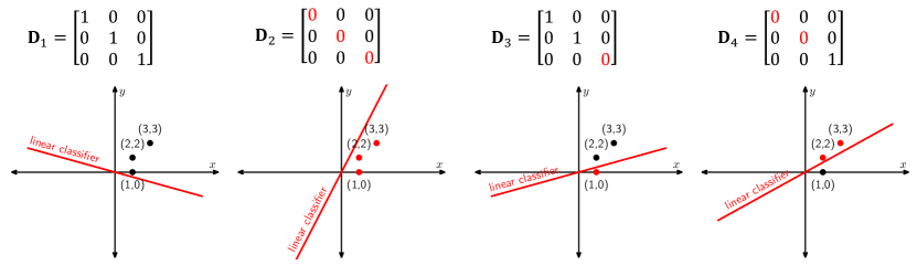
Figure 3: Illustration of possible hyperplane arrangements that determine the diagonal matrices $\mathbf{D}_{i}$. Here, we have three samples in two dimensions and we want to separate these samples with a linear classifier. $\mathbf{D}_{i}$ basically encodes information regarding which side of the linear classifier samples lie.

Since ReLU masks the negative entries of inputs, we have the following equivalent representation

$$\left(\left({\bf X}\mathbf{W}_{1}\right)_{+}\mathbf{w}_{2}\right)_{+}=\left(\sum_{j_{1}=1}^{m_{1}}\left({\bf X}\mathbf{w}_{1j_{1}}\right)_{+}w_{2j_{1}}\right)_{+} =\left(\sum_{j_{1}=1}^{m_{1}}\left({\bf X}\bar{\mathbf{w}}_{j_{1}}\right)_{+}\mathcal{I}_{j_{1}}\right)_{+}$$

$$=\mathbf{D}_{2}\sum_{j_{1}=1}^{m_{1}}\mathcal{I}_{j_{1}}\mathbf{D}_{1j_{1}}{\bf X}\bar{\mathbf{w}}_{j_{1}},$$ (7)

where $\bar{\mathbf{w}}_{j_{1}}=|w_{2j_{1}}|\mathbf{w}_{1j_{1}}$, $\mathcal{I}_{j_{1}}=\mathrm{sign}(w_{2j_{1}})\in\{-1,+1\}$, and we use the following alternative representation for ReLU (see Figure 3 for a two dimensional visualization)

$$\left({\bf X}\mathbf{w}\right)_{+}=\mathbf{D}{\bf X}\mathbf{w}~{}\iff~{}\begin{split}&\mathbf{D}{\bf X}\mathbf{w}\geq 0\\ &(\mathbf{I}_{n}-\mathbf{D}){\bf X}\mathbf{w}\leq 0\end{split}~{}\iff~{}(2\mathbf{D}-\mathbf{I}_{n}){\bf X}\mathbf{w}\geq 0,$$

​​where $\mathbf{D}\in\mathbb{R}^{n\times n}$ is a diagonal matrix of zeros/ones, i.e., $\mathbf{D}_{ii}\in\{0,1\}$. Therefore, we first enumerate all possible signs and diagonal matrices for the ReLU layers and denote them as $\mathcal{I}_{j_{1}}$, $\mathbf{D}_{1ij_{1}}$ and $\mathbf{D}_{2l}$ respectively, where $j_{1}\in[m_{1}],i\in[P_{1}],l\in[P_{2}]$. Here, $\mathbf{D}_{1ij_{1}}$ and $\mathbf{D}_{2l}$ denotes the masking/diagonal matrices for the first and second ReLU layers, respectively and $P_{1}$ and $P_{2}$ are the number diagonal matrices in each layer as detailed in Section A.10. Then, we convert the non-convex constraints in (6) to convex constraints using $\mathbf{D}_{1ij_{1}}$, $\mathbf{D}_{2l}$ and $\mathcal{I}_{j_{1}}$.

Using the representation in (3), we then take the dual of (6) to obtain the convex bidual of the primal problem (4) as detailed in the theorem below.

Theorem 1.

The non-convex training problem in (4) can be cast as the following convex program

$$\min_{\mathbf{z},\mathbf{z}^{\prime}\in\mathcal{C}}\mathcal{L}\left(\tilde{{\bf X}}(\mathbf{z}-\mathbf{z}^{\prime}),\mathbf{y}\right)+\frac{\beta}{\sqrt{m_{2}}}(\|\mathbf{z}\|_{F,1}+\|\mathbf{z}^{\prime}\|_{F,1}),$$ (8)

where $\|\cdot\|_{F,1}$ denotes a $d\times m_{1}$ dimensional group Frobenius norm operator such that given a vector $\mathbf{u}\in\mathbb{R}^{dm_{1}P}$, $\|\mathbf{u}\|_{F,1}:=\sum_{i=1}^{P}\|\mathbf{U}_{i}\|_{F}$, where $\mathbf{U}_{i}\in\mathbb{R}^{d\times m_{1}}$ are reshaped partitions of $\mathbf{u}$. Moreover, the convex set $\mathcal{C}$ is defined as

$$\mathcal{C}:=\{\mathbf{z}:\mathbf{z}_{ij_{1}l}^{{s}}\in\mathcal{C}_{il}^{s},\forall i\in[P_{1}],l\in[P_{2}],s\in[M]\}$$

$$\mathcal{C}_{il}^{s}:=\bigg{\{}\{\mathbf{w}_{j_{1}}\}_{j_{1}}:(2\mathbf{D}_{2l}-\mathbf{I}_{n})\sum_{j_{1}=1}^{m_{1}}\mathcal{I}_{ij_{1}l}^{s}\mathbf{D}_{1ij_{1}}{\bf X}\mathbf{w}_{j_{1}}\geq 0,(2\mathbf{D}_{1ij_{1}}-\mathbf{I}_{n}){\bf X}\mathbf{w}_{j_{1}}\geq 0,\forall j_{1}\in[m_{1}]\bigg{\}}$$

where $\mathcal{I}_{ij_{1}l}^{s}\in\{+1,-1\}$, $M=2^{m_{1}}$, and $\mathbf{z},\mathbf{z}^{\prime}\in\mathbb{R}^{dm_{1}MP_{1}P_{2}}$ are constructed by stacking $\mathbf{z}_{ij_{1}l}^{{s}},\mathbf{z}_{ij_{1}l}^{{s^{\prime}}}\in\mathbb{R}^{d}$, $\forall i\in[P_{1}],l\in[P_{2}],j_{1}\in[m_{1}],s\in[M]$, respectively. Also, the effective data matrix $\tilde{{\bf X}}\in\mathbb{R}^{n\times dm_{1}MP_{1}P_{2}}$ is defined as $\tilde{{\bf X}}:=\mathbf{I}_{M}\otimes\tilde{{\bf X}}_{s}$ and

$$\tilde{{\bf X}}_{s}:=\begin{bmatrix}\mathbf{D}_{21}\mathbf{D}_{111}{\bf X}\;\ldots\;\mathbf{D}_{2l}\mathbf{D}_{1ij_{1}}{\bf X}\;\ldots\;\mathbf{D}_{2P_{2}}\mathbf{D}_{1P_{1}m_{1}}{\bf X}\end{bmatrix}.$$

We next derive a mapping between the convex program (8) and the non-convex architecture (4).

Proposition 1.

An optimal solution to the non-convex parallel network training problem in (4), denoted as $\{\mathbf{W}_{1k}^{*},\mathbf{w}_{2k}^{*},w_{3k}^{*}\}_{k=1}^{K}$, can be recovered from an optimal solution to the convex program in (8), i.e., $\{\mathbf{z}^{*},\mathbf{z}^{\prime^{*}}\}$ via a closed-form mapping. Therefore, we prove a mapping between the parameters of the parallel network in Figure 2 and its convex equivalent.

Next, we prove that the convex program in (8) can be globally optimized with a polynomial-time complexity given ${\bf X}$ has fixed rank, i.e., $\mathrm{rank}({\bf X})=r<\min\{n,d\}$.

Proposition 2.

Given a data matrix such that $\mathrm{rank}({\bf X})=r<\min\{n,d\}$, the convex program in (8) can be globally optimized via standard convex solvers with $\mathcal{O}(d^{3}m_{1}^{3}m_{2}^{3}2^{3(m_{1}+1)m_{2}}n^{3(m_{1}+1)r})$ complexity, which is a polynomial-time complexity in terms of $n,d$. Note that here globally optimizing the training objective means to achieve the exact global minimum up to any arbitrary machine precision or solver tolerance.

Below, we show that the complexity analysis in Proposition 2 extends to arbitrarily deep networks.

Corollary 1.

The same analysis can be readily applied to arbitrarily deep networks. Therefore, given $\mathrm{rank}({\bf X})=r<\min\{n,d\}$, we prove that $L$-layer architectures can be globally optimized with $\mathcal{O}\left(d^{3}\left(\prod_{j=1}^{L-2}m_{j}^{3}\right)2^{3\sum_{j=1}^{L-1}m_{j}}n^{3r\left(1+\sum_{l=1}^{L-2}\prod_{j=1}^{l}m_{j}\right)}\right)$, which is polynomial in $n,d$.

(a) Objective value ($\downarrow$)

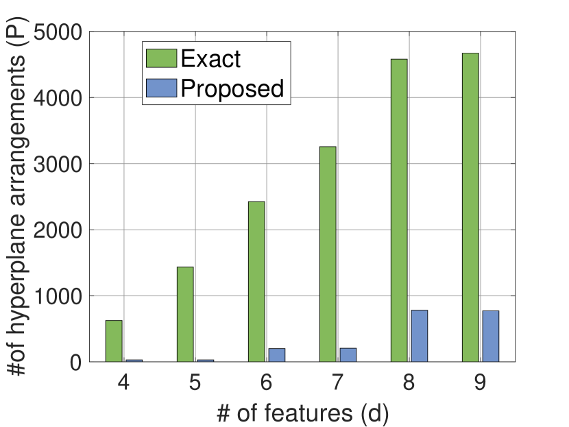
(b) $\#$ of hyperplane arrangements ($P$)

Figure 4: Verification of Theorem 2 and Remark 2. We train a parallel network using the convex program in Theorem 1 with $\ell_{2}$ loss on a toy dataset with $n=15$, $\beta=0.1$, $m_{2}=1$, and the low-rank approximation $r=\lfloor\frac{d}{2}\rfloor$. To obtain a low-rank model, we first sample a data matrix from a standard normal Gaussian distribution and then set $\sigma_{r+1}=\ldots=\sigma_{d}=1$. Please see the subsection for low rank models in Section 4 for more details.

3.1 Polynomial-time training for arbitrary data

Based on Corollary 1, exponential complexity is unavoidable for deep networks when the data matrix is full rank, i.e., $\mbox{rank}({\bf X})=\min\{n,d\}$. Thus, we propose a low rank approximation to the model in (4). We first denote the rank-$r$ approximation of ${\bf X}$ as $\hat{{\bf X}}_{r}$ such that $\|{\bf X}-\hat{{\bf X}}_{r}\|_{2}\leq\sigma_{r+1}$, where $\sigma_{r+1}$ represents the $(r+1)^{th}$ largest singular value of ${\bf X}$. Then, we have the following result.

Theorem 2.

Given an $R$-Lipschitz convex loss function $\mathcal{L}\left(\cdot,\mathbf{y}\right)$, the regularized training problem

$$p_{3}^{*}=\min_{\theta\in\Theta}~{}\mathcal{L}\left(f_{\theta}({\bf X}),\mathbf{y}\right)+\beta\sum_{k=1}^{K}\sqrt{\sum_{j_{1},j_{2}}\|\mathbf{w}_{1kj}\|_{2}^{2}w_{2kj_{1}j_{2}}^{2}w_{3kj_{2}}^{2}}\,,$$ (9)

can be solved using the data matrix $\hat{{\bf X}}_{r}$ to achieve the following optimality guarantee

$$p_{3}^{*}\leq p_{r}\leq p_{3}^{*}\left(1+\frac{\sqrt{m_{1}m_{2}}R\sigma_{r+1}}{\beta}\right)^{2},$$ (10)

where $p_{r}$ denotes the objective value achieved by the parameters trained using $\hat{{\bf X}}_{r}$.

Remark 2.

Theorem 1 and 2 imply that for a given arbitrary rank data matrix ${\bf X}$, the regularized training problem in (4) can be approximately solved by convex solvers to achieve a worst-case approximation $p_{3}^{*}\left(1+\frac{\sqrt{m_{1}m_{2}}R\sigma_{r+1}}{\beta}\right)^{2}$ with complexity $\mathcal{O}(d^{3}m_{1}^{3}2^{3(m_{1}+1)}n^{3(m_{1}+1)r})$, where $r\ll\min\{n,d\}$. Therefore, even for full rank data matrices where the complexity is exponential in $n$ or $d$, one can approximately solve the convex program in (8) in polynomial-time. Moreover, we remark that the approximation error proved in Theorem 2 can be arbitrarily small for practically relevant problems. As an example, consider a parallel network training problem with $\ell_{2}$ loss function, then the upperbound becomes $(1+\frac{\sqrt{m_{1}m_{2}}\sigma_{r+1}}{\beta})^{2}$, which is typically close to one due to fast decaying singular values in practice (see Figure 4).

3.2 Representational power: Two versus three layers

Here, we provide a complete explanation for the representational power of three-layer networks by comparing with the two-layer results in [6]. We first note that three-layer networks have substantially higher expressive power due to the non-convex interactions between hidden layers as detailed in [39, 40]. Furthermore, [41] show that layerwise training of three-layer networks can achieve comparable performance to deeper models, e.g., VGG-11, on Imagenet. There exist several studies analyzing two-layer networks, however, despite their empirical success, a full theoretical understanding and interpretation of three-layer networks is still lacking in the literature. In this work, we provide a complete characterization for three-layer networks through the lens of convex optimization theory. To understand their expressive power, we compare our convex program for three-layer networks in (8) with its two-layer counterpart in [6].

[6] analyzes two-layer networks with one ReLU layer, so that the data matrix ${\bf X}$ is multiplied with a single diagonal matrix (or hyperplane arrangement) $\mathbf{D}_{i}$. Thus, the effective data matrix is in the form of $\tilde{{\bf X}}_{s}=[\mathbf{D}_{1}{\bf X}\,\ldots\,\mathbf{D}_{P}{\bf X}]$. However, since our convex program in (8) has two nonlinear ReLU layers, the composition of these two-layer can generate substantially more complex features via locally linear variables $\{\mathbf{w}_{ij_{1}l}^{s}\}$ multiplying the $d$-dimensional blocks of the columns of the effective data matrix $\tilde{{\bf X}}_{s}$ in Theorem 1. Although this may seem similar to the features in [21], here, we have $2^{m_{1}}$ variables for each linear region unlike [21] which employ 2 variables per linear region. Moreover, [21] only considers the case where the second hidden layer has only one neuron, i.e., $m_{2}=1$, which is not a standard deep networks. Hence, we exactly describe the impact of having one more ReLU layer and its contribution to the representational power of the network.

Table 2: Training objective of a three-layer parallel network trained with non-convex SGD (5 independent initialization trials) on a toy dataset with $(n,d,m_{1},m_{2},\beta,\text{batch size})=(5,2,3,1,0.002,5)$, where the convex program in (8) are solved via the interior point solvers in CVX/CVXPY.

Method	Non-convex SGD					Convex(Ours)
	Run #1	Run #2	Run #3	Run #4	Run #5
$\bm{K=5}$ Training objective	$0.0221$	$0.0239$	$0.0031$	$0.0027$	$0.0027$	$\mathbf{0.0007}$
Time(s)	$11.62$	$11.62$	$11.62$	$11.62$	$11.62$	$\mathbf{4.947}$
$\bm{K=20}$ Training objective	$0.0010$	$0.0027$	$0.0009$	$0.0010$	$0.0027$	$\mathbf{0.0007}$
Time(s)	$44.37$	$44.37$	$44.37$	$11.55$	$44.37$	$\mathbf{4.947}$
$\bm{K=40}$ Training objective	$0.0008$	$0.0009$	$0.0009$	$0.0009$	$0.0008$	$\mathbf{0.0007}$
Time(s)	$91.87$	$91.87$	$91.87$	$91.87$	$91.87$	$\mathbf{4.947}$

4 Experiments

In this section, we present numerical experiments corroborating our theory.

Low rank model in Theorem 2: To validate our claims, we generate a synthetic dataset as follows. We first randomly generate a set of layer weights for a parallel ReLU network with $K=5$ sub-networks by sampling from a standard normal distribution. We then obtain the labels as $\mathbf{y}=\sum_{k}\left(\left({\bf X}\mathbf{W}_{1k}\right)_{+}\mathbf{W}_{2k}\right)_{+}\mathbf{w}_{3k}+0.1\bm{\epsilon}$, where $\bm{\epsilon}\sim N(\mathbf{0},\mathbf{I}_{n})$. To promote a low rank structure in the data, we first sample a matrix from the standard normal distribution and then set $\sigma_{r+1}=\ldots=\sigma_{d}=1$. We consider a regression framework with $\ell_{2}$ loss and $(n,r,\beta,m_{1},m_{2})=(15,d/2,0.1,1,1)$ and present the numerical results in Figure 4. Here, we observe that the low rank approximation of the objective $p_{r}$ is closer to $p_{3}^{*}$ than the worst-case upper-bound predicted by Theorem 2. However, in Figure 4(b), the low rank approximation provides a significant reduction in the number of hyperplane arrangements, and therefore in the complexity of solving the convex program.

Toy dataset: We use a toy dataset with $5$ samples and $2$ features, i.e., $(n,d)=(5,2)$. To generate the dataset, we forward propagate i.i.d. samples from a standard normal distribution, i.e., $\mathbf{x}_{i}\sim\mathcal{N}(\mathbf{0},\mathbf{I}_{d})$, through a parallel network with $3$ layers, $5$ sub-networks, and $3$ neurons, i.e., $(L,K,m_{1},m_{2})=(3,5,3,1)$. We then train the parallel network in (4) on this toy dataset using both our convex program (8) and non-convex SGD. We provide the training objective and wall-clock time in Table 2, where we particularly include $5$ initialization trials for SGD. This experiment shows that when the number of sub-networks $K$ is small, SGD trials fail to converge to the global minimum achieved by our convex program. However, as we increase $K$, the number of trials converging to global minimum gradually increases. Therefore, we show the benign overparameterization impact.

Image classification: We conduct experiments on benchmark image datasets, namely CIFAR-10 [42] and Fashion-MNIST [43]. We particularly consider a ten class classification task and use a parallel network with $40$ sub-networks and $100$ hidden neurons, i.e., $(K,m_{1},m_{2})=(40,100,1)$. In Figure 5, we plot the test accuracies against wall-clock time, where we include several different optimizers as well as SGD. Moreover, we include a parallel network trained with SGD/Adam and Weight Decay (WD) regularization to show the effectiveness of path regularization in (4). We first note that our convex approach achieves both faster convergence and higher final test accuracies for both dataset. However, the performance gain for Fashion-MNIST seems to be significantly less compared to the CIFAR-10 experiment. This is due to the nature of these datasets. More specifically, since CIFAR-10 is a much more challenging dataset, the baseline accuracies are quite low (around $\sim 50\%$) unlike Fashion-MNIST with the baseline accuracies around $\sim 90\%$. Therefore, the accuracy improvement achieved by the convex program seems low in Figure 5(b). We also observe that weight decay achieves faster convergence rates however path regularization yields higher final test accuracies. It is normal to have faster convergence with weight decay since it can be incorporated into gradient-based updates without any computational overhead.

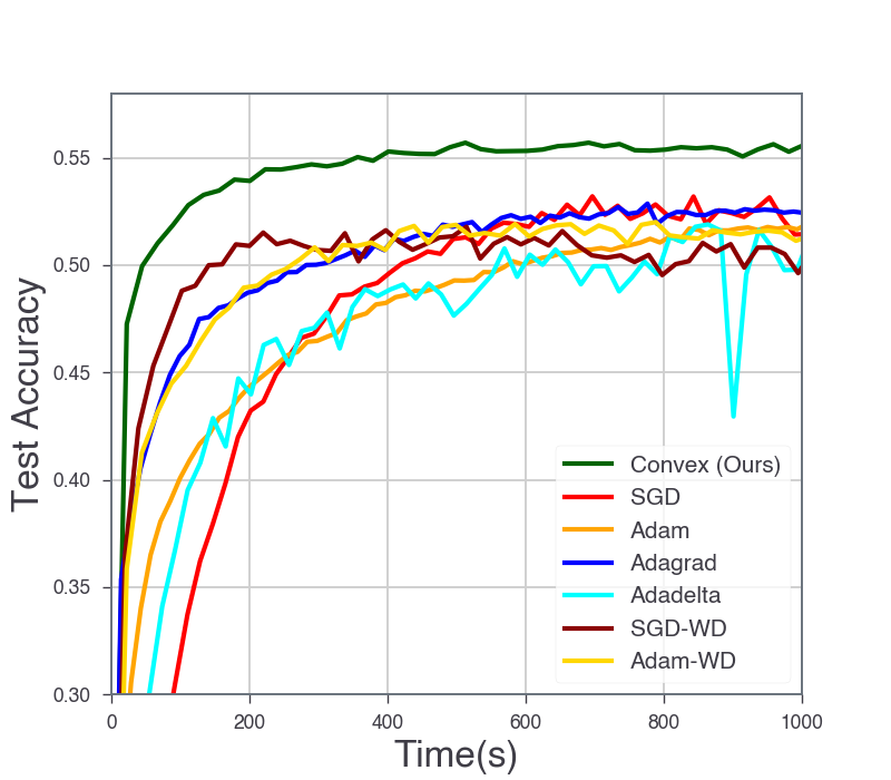
(a) CIFAR-10

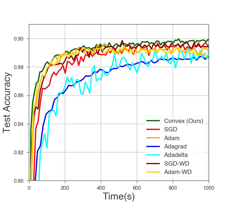
(b) Fashion-MNIST

Figure 5: Accuracy of a three-layer architecture trained using the non-convex formulation (4) and the proposed convex program (8), where we use (a) CIFAR-10 with $(n,d,m_{1},m_{2},K,\beta,\text{batch size})=(5\text{x}10^{4},3072,100,1,40,10^{-3},10^{3})$ and (b) Fashion-MNIST with $(n,d,m_{1},m_{2},K,\beta,\text{batch size})=(6\text{x}10^{4},784,100,1,40,10^{-3},10^{3})$. We note that the convex model is trained using (a) SGD and (b) Adam.

5 Related Work

Parallel neural networks were previously investigated by [22, 23]. Although these studies provided insights into the solutions, they require impractical assumptions, e.g., sparsity among sub-networks in Theorem 1 of [23]) and linear activations and hinge loss assumptions in [22].

Recently, [6] studied weight decay regularized two-layer ReLU network training problems and introduced polynomial-time trainable convex formulations. However, their analysis is restricted to standard two-layer ReLU networks, i.e., in the form of $f_{\theta}({\bf X})=\left({\bf X}\mathbf{W}_{1}\right)_{+}\mathbf{w}_{2}$. The reasons for this restriction is that handling more than one ReLU layer is a substantially more challenging optimization problem. As an example, a direct extension of [6] to three-layer NNs will yield doubly exponential complexity, i.e., $\mathcal{O}(n^{rn^{r}})$ for a rank-$r$ data matrix, due to the combinatorial behavior of multiple ReLU layers. Thus, they only examined the case with a single ReLU layer (see Table 1 for details and references in [6]). Additionally, since they only considered standard two-layer ReLU networks, their analysis is not valid for a broader range of NN-based architectures as detailed in Remark 1. Later on, [21] extended this approach to three-layer ReLU networks. However, since they analyzed $\ell_{2}$-norm regularized training problem, they had to put unit Frobenius norm constraints on the first layer weights, which does not reflect the settings in practice. In addition, their analysis is restricted to the networks with a single neuron in the second layer (i.e. $m_{2}=1$) that is in the form of $f_{\theta}({\bf X})=\sum_{k}\left(\left({\bf X}\mathbf{W}_{1k}\right)_{+}\mathbf{w}_{2k}\right)_{+}w_{3k}$. Since this architecture only allows a single neuron in the second layer, each sub-network $k$ has an expressive power that is equivalent to a standard two-layer network rather than three-layer. This can also be realized from the definition of the constraint set $\mathcal{C}$ in Theorem 1. Specifically, the convex set $\mathcal{C}$ in [21] has decoupled constraints across the hidden layer index $j_{1}$ whereas our formulation sums the responses over hidden neurons before feeding through the next layer as standard deep networks do. Therefore, this analysis does not reflect the true power of deep networks with $L>2$. Moreover, the approach in [21] has exponential complexity when the data matrix has full rank, which is unavoidable.

However, we analyze deep neural networks in (1) without any assumption on the weights. Furthermore, we develop an algorithm which has fully polynomial-time complexity in data dimensions and prove strong global optimality guarantees for this algorithm in Theorem 2.

6 Concluding Remarks

We studied the training problem of path regularized deep parallel ReLU networks, which includes ResNets and standard deep ReLU networks as its special cases. We first showed that the non-convex training problem can be equivalently cast as a single convex optimization problem. Therefore, we achieved the following advantages over the training on the original non-convex formulation: 1) Since our model is convex, it can be globally optimized via standard convex solvers whereas the non-convex formulation trained with optimizers such as SGD might be stuck at a local minimum, 2) Thanks to convexity, our model does not require any sort of heuristics and additional tricks such as learning rate schedule and initialization scheme selection or dropout. More importantly, we proposed an approximation to the convex program to enable fully polynomial-time training in terms of the number of data samples $n$ and feature dimension $d$. Thus, we proved the polynomial-time trainability of deep ReLU networks without requiring any impractical assumptions unlike [6, 21]. Notice that we derive an exact convex program only for three-layer networks, however, recently [19] proved that strong duality holds for arbitrarily deep parallel networks. Therefore, a similar analysis can be extended to deeper networks to achieve an equivalent convex program, which is quite promising for future work. Additionally, although we analyzed fully connected networks in this paper, our approach can be directly extended to various NN architectures, e.g., threshold/binary networks [44], convolution networks [45], generative adversarial networks [46], NNs with batch normalization [47], autoregressive models [48], and Transformers [49, 50].

Supplementary Material

Appendix A Appendix

A.1 Additional numerical results and details

In this section, we provide new numerical results and detailed information about our experiments in the main paper.

Decision boundary plots in Figure 1: In order to visualize the capabilities of our convex training approach, we perform an experiment on the spiral dataset which is known to be challenging for 2-layer networks while 3-layer networks can readily interpolate the training data (i.e. exactly fit the training labels) [51]. As the baselines of our analysis, we include the two-layer convex training approach in [6] and recently introduced three-layer convex training approach (with weight decay regularization and several architectural and parametric assumptions) in [21]. As our experimental setup, we consider a binary classification task with $\mathbf{y}\in\{+1,-1\}^{n}$ and squared loss. We choose $(n,m_{1},m_{2},P_{1},P_{2},\beta)=(30,5,1,11,11,1e-4)$ and for [6] we use $P=50$ neurons/hyperplane arrangements. We also use CVPXY with MOSEK solver [52, 53, 54] to globally solve the convex programs. As demonstrated in Figure 1, baselines methods, especially [21], fit a function that is significantly different than the underlying spiral data distribution. This clearly shows that since [6] is restricted two-layer networks and [21] have multiple assumptions, i.e., unit Frobenius norm constraints on the layer weights ($\|\mathbf{W}_{lk}\|_{F}\leq 1,\forall l\in[L-2]$) and last hidden layer weights cannot be matrices ($\mathbf{w}_{(L-1)k}\in\mathbb{R}^{m_{L-2}}$), both baseline approaches fail to reflect true expressive power of deep networks ($L>2$). On the other hand, our convex training approach for path regularized networks fits a model that successfully describes the underlying data distribution for this challenging task.

Additional experiments: We also conduct experiments on several datasets available in UCI Machine Learning Repository [55], where we particularly selected the datasets from [56] such that $n\leq 500$. For these datasets, we consider a conventional binary classification framework with $(m_{1},m_{2},K,\beta)=(100,1,40,0.5)$ and compare the test accuracies of non-convex architectures trained with SGD and Adam with their convex counter parts in (8). For these experiments, we use the $80\%-20\%$ splitting ratio for the training and test sets. Furthermore, we train each algorithm long enough to reach training accuracy one. As shown in Table 3, our convex approach achieves higher or the same test accuracy compared to the standard non-convex training approach for most of the datasets (precisely $20$ and $19$ out of $21$ datasets for SGD and Adam, respectively). We also note that for this experiment, we used the unconstrained form in (11) with the approximate version in Remark 3.3 of [6].

Table 3: Test accuracies for UCI experiments ($(m_{1},m_{2},K,\beta)=(100,1,40,0.5)$ and $80\%-20\%$ training-test split). Here, we present the standard non-convex architectures and the proposed convex counterpart trained with SGD and Adam optimizers. If one approach achieves higher accuracy on a certain dataset, we display the corresponding accuracy value in bold font. We observe that our convex approach achieves either higher or the same accuracy for $20$ and $19$ datasets (out of $21$ datasets) when trained with SGD and Adam, respectively

			SGD		Adam
Dataset	$n$	$d$	Non-convex	Convex(Ours)	Non-convex	Convex(Ours)
acute-inflammation	$120$	$6$	$1.000$	$1.000$	$1.000$	$1.000$
acute-nephritis	$120$	$6$	$1.000$	$1.000$	$1.000$	$1.000$
balloons	$16$	$4$	${1.000}$	${1.000}$	$1.000$	$1.000$
breast-cancer	$286$	$9$	${0.690}$	$\mathbf{0.707}$	${0.655}$	$\mathbf{0.672}$
breast-cancer-wisc-prog	$198$	$33$	${0.750}$	$\mathbf{0.800}$	${0.800}$	$\mathbf{0.825}$
congressional-voting	$435$	$16$	${0.667}$	${0.667}$	${0.551}$	$\mathbf{0.597}$
conn-bench-sonar-mines-rocks	$208$	$60$	${0.714}$	$\mathbf{0.786}$	${0.738}$	$\mathbf{0.833}$
echocardiogram	$131$	$10$	${0.704}$	${0.704}$	${0.666}$	$\mathbf{0.703}$
fertility	$100$	$9$	${0.750}$	$\mathbf{0.800}$	${0.800}$	${0.800}$
haberman-survival	$306$	$3$	$0.710$	$\mathbf{0.774}$	${0.677}$	$\mathbf{0.709}$
heart-hungarian	$294$	$12$	${0.831}$	${0.831}$	${0.779}$	$\mathbf{0.813}$
hepatitis	$155$	$19$	${0.645}$	$\mathbf{0.710}$	${0.709}$	$\mathbf{0.741}$
ionosphere	$351$	$33$	${0.887}$	$\mathbf{0.901}$	$\mathbf{0.929}$	${0.887}$
molec-biol-promoter	$106$	$57$	${0.818}$	$0.818$	${0.727}$	$\mathbf{0.772}$
musk-1	$476$	$166$	$\mathbf{0.958}$	${0.927}$	$\mathbf{0.947}$	${0.927}$
parkinsons	$195$	$22$	${0.974}$	$\mathbf{1.000}$	${0.923}$	$\mathbf{1.000}$
pittsburg-bridges-T-OR-D	$102$	$7$	${0.952}$	${0.952}$	${0.809}$	$\mathbf{0.857}$
planning	$182$	$12$	${0.541}$	$\mathbf{0.568}$	${0.649}$	$\mathbf{0.703}$
statlog-heart	$270$	$13$	$0.759$	$\mathbf{0.796}$	${0.759}$	$\mathbf{0.833}$
trains	$10$	$29$	$1.000$	$1.000$	${1.000}$	${1.000}$
vertebral-column-2clases	$310$	$6$	${0.806}$	$\mathbf{0.839}$	${0.758}$	$\mathbf{0.822}$
Highest test accuracy				20/21		19/21

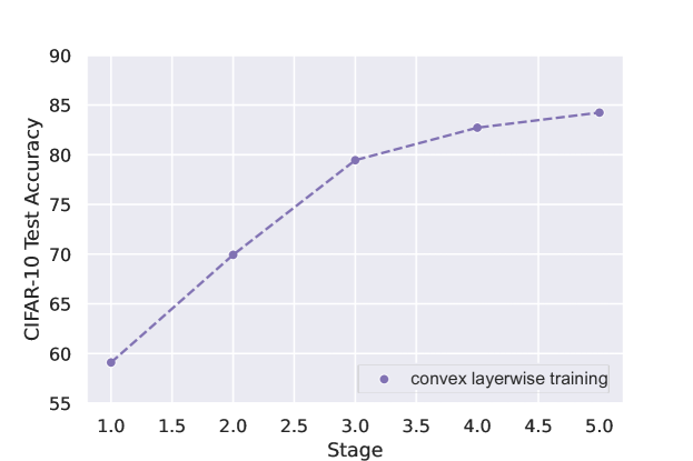
Figure 6: Test accuracy for convex layerwise training, where each stage is our three-layer convex formulation in Theorem 1. Here, we train three-layer neural networks sequentially using convex optimization to build deep networks.

Details for the experiments in Table 2 and Figure 5: We first note that for the experiments in Table 2, we use CVX/CVPXY [52, 53, 54] to globally solve the proposed convex program in (8). For these experiments, we use a laptop with i7 processor and 16GB of RAM. In order to tune the learning rate of SGD/GD, we first perform training with a bunch of learning different learning rates and select the one with the best performance on the validation datasets, which is $0.005$ in these experiments.

For comparatively larger scale image classification experiments in Figure 5, we utilize a cluster GPU with 50GB of memory. However since the equivalent convex program in (8) has constraint which are challenging to handle for these datasets, we propose the following unconstrained convex problem which has the same global minima with the constrained version as discussed in [48]

$$\min_{\mathbf{z},\mathbf{z}^{\prime}\in\mathbb{R}^{dm_{1}MP_{1}P_{2}}}\mathcal{L}\left(\tilde{{\bf X}}\left(\mathbf{z}^{\prime}-\mathbf{z}\right),\mathbf{y}\right)+\beta\left(\|\mathbf{z}\|_{G,1}+\|\mathbf{z}^{\prime}\|_{G,1}\right)+\lambda\left(h_{\mathcal{C}}(\mathbf{z})+h_{\mathcal{C}}(\mathbf{z}^{\prime})\right)$$ (11)

where $\lambda>0$ coefficient to penalize the violated constraints and $h_{\mathcal{C}}(\mathbf{z})$ is a function to sum the absolute value of all constraint violations defined as

$$h_{\mathcal{C}}(\mathbf{z}):=\mathbf{1}^{T}\sum_{i,j_{1},l,s}\left(\left(-(2\mathbf{D}_{1ij_{1}}-\mathbf{I}_{n}){\bf X}\mathbf{z}_{ij_{1}l}^{s}\right)_{+}\right)+\mathbf{1}^{T}\sum_{i,l,s}\left(-\sum_{j_{1}}\mathcal{I}_{ij_{1}l}^{s}(2\mathbf{D}_{2l}-\mathbf{I}_{n})\mathbf{D}_{1ij_{1}}{\bf X}\mathbf{z}_{ij_{1}l}^{s}\right)_{+}.$$

Thus, we obtain an unconstrained version of convex optimization problem (11), where one can use commonly employed first-order gradient based optimizers, e.g., SGD and Adam, available in deep learning libraries such PyTorch and Tensorflow. For both CIFAR-10 and Fashion-MNIST, we use the same training and test splits in the original datasets. We again perform a grid search to tune the learning rate, where the best performance is achieved by the following choices

$$(\mu_{Convex},\mu_{SGD},\mu_{Adam},\mu_{Adagrad},\mu_{Adadelta},\mu_{SGD}^{WD})=(5e-7,5e-3,2e-5,2e-3,3e-1,1)$$

and

$$(\mu_{Convex},\mu_{SGD},\mu_{Adam},\mu_{Adagrad},\mu_{Adadelta},\mu_{SGD}^{WD})=(1e-5,2e-1,2e-3,1e-2,3,1)$$

as the learning rates for CIFAR-10 and Fashion-MNIST, respectively. We choose the momentum coefficient of the SGD optimizer as $0.9$. In addition to this, we set $P_{1}P_{2}=K$ and $\lambda=1e-5$.

More importantly, we remark that these experiments are performed by using a small sampled subset of hyperplane arrangements rather than sampling all possible arrangements as detailed in Remark 3.3 of [6]. In particular, we first generate random weight matrices from a multivariate standard normal distribution and then solve the convex program using only the arrangements of the sampled weight matrices.

Details for the experiments in Figure 6: Layerwise training with shallow neural networks was proven to work remarkably well. Particularly, [41] shows that one can train three-layer neural networks sequentially to build deep networks that outperform end-to-end training with SOTA architectures. In Figure 6, we apply this layerwise training procedure with our convex training approach. In particular, each stage in this figure is our three-layer convex formulation in Theorem 1. Here, we use the same experimental setting in the previous section. We observe that making the network deeper by stacking convex layers resulted in significant performance improvements. Specificaly, at the fifth stage, we achieved almost $85\%$ accuracy for CIFAR-10 unlike below $60\%$ accuracies in Figure 5.

A.2 Parallel ReLU networks

The parallel networks $f_{\theta}({\bf X})$ models a wide range of NNs in practice. As an example, standard NNs and ResNets [33] are special cases of this network architecture. To illustrate this, let us consider a parallel ReLU with two sub-networks and four layers, i.e., $K=2$ and $L=4$. If we set $\mathbf{W}_{lk}=\mathbf{W}_{l}\forall k\in[2],l\in[4]$ then our architecture reduces to a standard four-layer network

$$\sum_{k=1}^{2}\left(\left(\left({\bf X}\mathbf{W}_{1k}\right)_{+}\mathbf{W}_{2k}\right)_{+}\mathbf{W}_{3k}\right)_{+}\mathbf{w}_{4k}=\left(\left(\left({\bf X}\mathbf{W}_{1}\right)_{+}\mathbf{W}_{2}\right)_{+}\mathbf{W}_{3}\right)_{+}\mathbf{w}_{4},$$

where $\mathbf{W}_{1}\in\mathbb{R}^{d\times m_{1}},\mathbf{W}_{2}\in\mathbb{R}^{m_{1}\times m_{2}},\mathbf{W}_{3}\in\mathbb{R}^{m_{2}\times m_{3}},\mathbf{w}_{4}\in\mathbb{R}^{m_{3}}$. For ResNets, we first remark that since residual blocks are usually used after a ReLU activation function, which is positively homogeneous of degree one, in practice, each residual block takes only nonnegative entries as its inputs. Thus, we can assume ${\bf X}\in\mathbb{R}_{+}^{n\times d}$ without loss of generality. We also assume that weights obey the following form: $\mathbf{W}_{11}=\mathbf{W}_{1}$, $\mathbf{W}_{21}=\mathbf{W}_{2}$, $\mathbf{W}_{12}=\mathbf{W}_{22}=\mathbf{I}_{d}$, $\mathbf{W}_{31}=\mathbf{W}_{32}=\mathbf{W}_{3}$, and $\mathbf{w}_{41}=\mathbf{w}_{42}=\mathbf{w}_{4}$ then

$$f_{\theta}({\bf X}) =\sum_{k=1}^{2}\left(\left(\left({\bf X}\mathbf{W}_{1k}\right)_{+}\mathbf{W}_{2k}\right)_{+}\mathbf{W}_{3k}\right)_{+}\mathbf{w}_{4k}=\left(\left(\left({\bf X}\mathbf{W}_{1}\right)_{+}\mathbf{W}_{2}\right)_{+}\mathbf{W}_{3}\right)_{+}\mathbf{w}_{4}+\left({\bf X}\mathbf{W}_{3}\right)_{+}\mathbf{w}_{4}$$

which is a shallow ResNet as demonstrated in Figure 1 of [25].

A.3 Proof of Lemma 1

Let us first define $r_{kj_{L-1}}:=\sqrt{\sum_{j_{1},\ldots,j_{L-2}}\left(\|\mathbf{w}_{1kj_{1}}\|_{2}^{2}\prod_{l=2}^{L-1}w_{lkj_{l-1}j_{l}}^{2}\right)}>0$. Notice that if $r_{kj_{L-1}}=0$, this means that $k^{th}$ sub-network does not contribute the output of the parallel network in (1). Therefore, we can remove the paths with $r_{kj_{L-1}}=0$ without loss of generality. Now, we use the following change of variable

$$\mathbf{W}_{lk}^{\prime}=\mathbf{W}_{lk},\forall l\in[L-2],\,\mathbf{w}_{(L-1)kj_{L-1}}^{\prime}=\frac{\mathbf{w}_{(L-1)kj_{L-1}}}{r_{kj_{L-1}}},\forall l\in[L-1],\;w_{Lkj_{L-1}}^{\prime}=r_{kj_{L-1}}w_{Lkj_{L-1}}.$$

We now note that

$$\sum_{j_{1},\ldots,j_{L-2}}\left(\|\mathbf{w}_{1kj_{1}}^{\prime}\|_{2}^{2}\prod_{l=2}^{L-1}w_{lkj_{l-1}j_{l}}^{\prime^{2}}\right)=\frac{1}{r_{kj_{L-1}}^{2}}\sum_{j_{1},\ldots,j_{L-2}}\left(\|\mathbf{w}_{1kj_{1}}\|_{2}^{2}\prod_{l=2}^{L-1}w_{lkj_{l-1}j_{l}}^{2}\right)=1.$$

Then, (2) can be restated as follows

$$p_{L}^{*} =\min_{\{\{\mathbf{W}_{lk}\}_{l=1}^{L}\}_{k=1}^{K}}\mathcal{L}\left(\sum_{k=1}^{K}\left(\left({\bf X}\mathbf{W}_{1k}\right)_{+}\ldots\mathbf{W}_{(L-1)k}\right)_{+}\mathbf{w}_{Lk},\mathbf{y}\right)+\beta\sum_{k=1}^{K}\sqrt{\sum_{j_{1}\ldots,j_{L}}\left(\|\mathbf{w}_{1kj_{1}}\|_{2}^{2}\prod_{l=2}^{L}w_{lkj_{l-1}j_{l}}^{2}\right)}$$

$$=\min_{\begin{subarray}{c}\{\{\mathbf{W}_{lk}\}_{l=1}^{L-1}\}_{k=1}^{K}\\ \{\mathbf{w}_{Lk}^{\prime}\}_{k=1}^{K}\end{subarray}}\mathcal{L}\left(\sum_{k=1}^{K}\sum_{j_{L-1}}\frac{\left(\left({\bf X}\mathbf{W}_{1k}\right)_{+}\ldots\mathbf{w}_{(L-1)kj_{L-1}}\right)_{+}}{r_{kj_{L-1}}}w_{Lkj_{L-1}}^{\prime},\mathbf{y}\right)$$

$$+\beta\sum_{k=1}^{K}\sqrt{\sum_{j_{L-1}}w_{Lkj_{L-1}}^{\prime^{2}}\frac{\sum_{j_{1},\ldots,j_{L-2}}\left(\|\mathbf{w}_{1kj_{1}}\|_{2}^{2}\prod_{l=2}^{L-1}w_{lkj_{l-1}j_{l}}^{2}\right)}{r_{kj_{L-1}}^{2}}}$$

$$=\min_{\begin{subarray}{c}\{\{\mathbf{W}_{lk}\}_{l=1}^{L-1}\}_{k=1}^{K}\\ \{\mathbf{w}_{Lk}^{\prime}\}_{k=1}^{K}\end{subarray}}\mathcal{L}\left(\sum_{k=1}^{K}\sum_{j_{L-1}}\left(\left({\bf X}\mathbf{W}_{1k}\right)_{+}\ldots r_{kj_{L-1}}^{-1}\mathbf{w}_{(L-1)kj_{L-1}}\right)_{+}w_{Lkj_{L-1}}^{\prime},\mathbf{y}\right)+\beta\sum_{k=1}^{K}\|\mathbf{w}_{Lk}^{\prime}\|_{2}$$

$$=\min_{\begin{subarray}{c}\{\{\mathbf{W}_{lk}^{\prime}\}_{l=1}^{L}\}_{k=1}^{K}\\ (\mathbf{W}_{1k}^{\prime},\ldots,\mathbf{W}_{(L-1)k}^{\prime})\in\Theta_{s},\forall k\end{subarray}}\mathcal{L}\left(\sum_{k=1}^{K}\left(\left({\bf X}\mathbf{W}_{1k}^{\prime}\right)_{+}\ldots\mathbf{W}_{(L-1)k}^{\prime}\right)_{+}\mathbf{w}_{Lk}^{\prime},\mathbf{y}\right)+\beta\sum_{k=1}^{K}\|\mathbf{w}_{Lk}^{\prime}\|_{2},$$

where $\Theta_{s}:=\left\{(\mathbf{W}_{1},\ldots,\mathbf{W}_{L-1}):\sum_{j_{1},\ldots,j_{L-2}}\left(\|\mathbf{w}_{1j_{1}}\|_{2}^{2}\prod_{l=2}^{L-1}w_{lj_{l-1}j_{l}}^{2}\right)=1,\,\forall j_{L-1}\in[m_{L-1}]\right\}$.

We also note that one can relax the equality constraint as an inequality constraint without loss of generality. This is basically due to the fact that if a constraint is not tight, i.e., strictly less than one, at the optimum then we can remove that constraint and make the corresponding output layer weight arbitrarily small via a simple scaling to make the objective value smaller. However, this would lead to a contradiction since this scaling further reduces the objective, which means that the initial set of layer weights (that yields a strict inequality in the constraints) are not optimal.

∎

A.4 Proof of Theorem 1

To obtain the bidual problem of (4), we first utilize semi-infinite duality theory as follows. We first compute the dual of (6) with respect to the dual parameter $\mathbf{v}$ to get

$$p_{\infty}^{*}:=\min_{\|\mathbf{w}_{3}\|_{2}\leq 1}\min_{\bm{\mu}}\mathcal{L}\left(\int_{\begin{subarray}{c}\theta\in\Theta_{s}\end{subarray}}\left(\left({\bf X}\mathbf{W}_{1}\right)_{+}\mathbf{W}_{2}\right)_{+}\mathbf{w}_{3}d{\mu}(\theta),\mathbf{y}\right)+\beta\|\bm{\mu}\|_{TV},$$ (12)

where $\|\bm{\mu}\|_{TV}$ denotes the total variation norm of the signed measure $\bm{\mu}$. Notice that (12) is an infinite-dimensional neural network training problem similar to the one studied in [38]. More importantly, this problem is convex since the model is linear with respect to the measure $\mu$ and the loss and regularization functions are convex [38]. Thus, we have no duality gap, i.e., $d_{3}^{*}=p_{\infty}^{*}$. In addition to this, even though (12) is an infinite-dimensional convex optimization problem, it reduces to a problem with at most $n+1$ neurons at the optimum due to Caratheodory’s theorem [35]. Therefore, (12) can be equivalently stated as the following finite-size convex optimization problem

$$p_{\infty}^{*} =\min_{\theta\in\Theta_{s}}\mathcal{L}\left(\sum_{k=1}^{K^{*}}\left(\left({\bf X}\mathbf{W}_{1k}\right)_{+}\mathbf{W}_{2k}\right)_{+}\mathbf{w}_{3k},\mathbf{y}\right)+\beta\sum_{k=1}^{K^{*}}\|\mathbf{w}_{3k}\|_{2}$$

$$=\min_{\theta\in\Theta_{s}}\mathcal{L}\left(f_{\theta}({\bf X}),\mathbf{y}\right)+\beta\sum_{k=1}^{K^{*}}\|\mathbf{w}_{3k}\|_{2},$$ (13)

where $K^{*}\leq n+1$. We further remark that given $K\geq K^{*}$, (A.4) and (5) are the same problems, which also proves strong duality as $p_{3}^{*}=p_{\infty}^{*}=d_{3}^{*}$. In the remainder of the proof, we show that using an alternative representation for the ReLU activation, we can achieve a finite-dimensional convex bidual formulation.

Now we restate the dual problem (6) as

$$d_{3}^{*}=\max_{\mathbf{v}}-\mathcal{L}^{*}(\mathbf{v})\text{ s.t. }\max_{\theta\in\Theta_{s}}\left\|\mathbf{v}^{T}\left(\left({\bf X}\mathbf{W}_{1}\right)_{+}\mathbf{W}_{2}\right)_{+}\right\|_{2}\leq\beta.$$ (14)

We first note that using the representation in (3), the dual constraint in (14) can be written as

$$\max_{\theta\in\Theta_{s}}\left\|\mathbf{v}^{T}\left(\left({\bf X}\mathbf{W}_{1}\right)_{+}\mathbf{W}_{2}\right)_{+}\right\|_{2}\leq\beta \iff\max_{\theta\in\Theta_{s}}\,\sqrt{\sum_{j_{2}=1}^{m_{2}}\left(\mathbf{v}^{T}\left(\left({\bf X}\mathbf{W}_{1}\right)_{+}\mathbf{w}_{2j_{2}}\right)_{+}\right)^{2}}\leq\beta$$

$$\iff\max_{\theta\in\Theta_{s}}\,\sqrt{m_{2}\left(\mathbf{v}^{T}\left(\left({\bf X}\mathbf{W}_{1}\right)_{+}\mathbf{w}_{2}\right)_{+}\right)^{2}}\leq\beta$$

$$\iff\max_{\begin{subarray}{c}\mathcal{I}_{j_{1}}\in\{\pm 1\}\end{subarray}}\max_{\theta\in\Theta_{s}}\,\sqrt{m_{2}\left(\mathbf{v}^{T}\left(\sum_{j_{1}=1}^{m_{1}}\mathcal{I}_{j_{1}}\left({\bf X}\mathbf{w}_{1j_{1}}|w_{2j_{1}}|\right)_{+}\right)_{+}\right)^{2}}\leq\beta$$

$$\iff\max_{\begin{subarray}{c}i\in[P_{1}]\\ l\in[P_{2}]\end{subarray}}\max_{\begin{subarray}{c}\mathcal{I}_{j_{1}}\in\{\pm 1\}\end{subarray}}\max_{\begin{subarray}{c}\{\mathbf{w}_{j_{1}}\}_{j_{1}}\in\mathcal{C}_{il}\end{subarray}}\,\sqrt{m_{2}}\left|\mathbf{v}^{T}\mathbf{D}_{2l}\sum_{j_{1}=1}^{m_{1}}\mathcal{I}_{j_{1}}\mathbf{D}_{1ij_{1}}{\bf X}\mathbf{w}_{j_{1}}\right|\leq\beta$$ (15)

where $\Theta_{s}=\{(\mathbf{W}_{1},\mathbf{W}_{2}):\sum_{j_{1}=1}^{m_{1}}\|\mathbf{w}_{1j_{1}}\|_{2}^{2}w_{2j_{1}j_{2}}^{2}\leq 1,\forall j_{2}\in[m_{2}]\}$, we apply a variable change as $\mathbf{w}_{j_{1}}=|w_{2j_{1}}|\mathbf{w}_{1j_{1}}$ and define the set $\mathcal{C}_{il}$ as

$$\mathcal{C}_{il}:= \{\{\mathbf{w}_{j_{1}}\}_{j_{1}}:(2\mathbf{D}_{2l}-\mathbf{I}_{n})\sum_{j_{1}=1}^{m_{1}}\mathcal{I}_{j_{1}}\mathbf{D}_{1ij_{1}}{\bf X}\mathbf{w}_{j_{1}}\geq 0,(2\mathbf{D}_{1ij_{1}}-\mathbf{I}_{n}){\bf X}\mathbf{w}_{j_{1}}\geq 0,\forall j_{1}\in[m_{1}],\sum_{j_{1}=1}^{m_{1}}\|\mathbf{w}_{j_{1}}\|_{2}^{2}\leq 1\}.$$

We also note that $P_{1}$ and $P_{2}$ denote the number of possible hyperplane arrangement for the first and second ReLU layer (see Appendix A.10 for details).

Then we have

$$\max_{\theta\in\Theta_{s}}\left\|\mathbf{v}^{T}\left(\left({\bf X}\mathbf{W}_{1}\right)_{+}\mathbf{W}_{2}\right)_{+}\right\|_{2}\leq\beta\iff\max_{\begin{subarray}{c}i\in[P_{1}]\\ l\in[P_{2}]\\ \mathcal{I}_{j_{1}}\in\{\pm 1\}\end{subarray}}\max_{\begin{subarray}{c}\{\mathbf{w}_{j_{1}}\}_{j_{1}}\in\mathcal{C}_{il}\end{subarray}}\,\sqrt{m_{2}}\left|\mathbf{v}^{T}\mathbf{D}_{2l}\sum_{j_{1}=1}^{m_{1}}\mathcal{I}_{j_{1}}\mathbf{D}_{1ij_{1}}{\bf X}\mathbf{w}_{j_{1}}\right|\leq\beta,\,$$

$$\iff\begin{split}\max_{\begin{subarray}{c}\{\mathbf{w}_{ij_{1}l}^{s}\}_{j_{1}}\in\mathcal{C}_{il}^{s}\end{subarray}}\,\sqrt{m_{2}}\mathbf{v}^{T}\mathbf{D}_{2l}\sum_{j_{1}=1}^{m_{1}}\mathcal{I}_{ij_{1}l}^{s}\mathbf{D}_{1ij_{1}}{\bf X}\mathbf{w}_{ij_{1}l}^{s}\leq\beta,\\ \max_{\begin{subarray}{c}\{\mathbf{w}_{ij_{1}l}^{s^{\prime}}\}_{j_{1}}\in\mathcal{C}_{il}^{s}\end{subarray}}\,-\sqrt{m_{2}}\mathbf{v}^{T}\mathbf{D}_{2l}\sum_{j_{1}=1}^{m_{1}}\mathcal{I}_{ij_{1}l}^{s^{\prime}}\mathbf{D}_{1ij_{1}}{\bf X}\mathbf{w}_{ij_{1}l}^{s^{\prime}}\leq\beta,\end{split},\;\forall i\in[P_{1}],\forall l\in[P_{2}],\forall s\in[M],$$

where we use $M:=|\{\pm 1\}^{m_{1}}|=2^{m_{1}}$ to enumerate all possible sign patterns $\{\mathcal{I}_{j_{1}}\}_{j_{1}=1}^{m_{1}}$ of size $m_{1}$. Using the equivalent representation above, we rewrite the dual (14) as

$$\max_{\begin{subarray}{c}\mathbf{v}\end{subarray}}-\mathcal{L}^{*}(\mathbf{v})\text{ s.t. } \max_{\begin{subarray}{c}\{\mathbf{w}_{ij_{1}l}^{s}\}_{j_{1}}\in\mathcal{C}_{il}^{s}\end{subarray}}\,\sqrt{m_{2}}\mathbf{v}^{T}\mathbf{D}_{2l}\sum_{j_{1}=1}^{m_{1}}\mathcal{I}_{ij_{1}l}^{s}\mathbf{D}_{1ij_{1}}{\bf X}\mathbf{w}_{ij_{1}l}^{s}\leq\beta,\;\forall i,l,s$$ (16)

$$\max_{\begin{subarray}{c}\{\mathbf{w}_{ij_{1}l}^{s^{\prime}}\}_{j_{1}}\in\mathcal{C}_{il}^{s}\end{subarray}}\,-\sqrt{m_{2}}\mathbf{v}^{T}\mathbf{D}_{2l}\sum_{j_{1}=1}^{m_{1}}\mathcal{I}_{ij_{1}l}^{s^{\prime}}\mathbf{D}_{1ij_{1}}{\bf X}\mathbf{w}_{ij_{1}l}^{s^{\prime}}\leq\beta,\;\forall i,l,s.$$ (17)

Since the problem above is convex and satisfies the Slater’s condition when all the parameters are set to zero, we have strong duality [36], and thus we can state (16) as

$$\min_{\begin{subarray}{c}\gamma_{il}^{s}\geq 0\\ \gamma_{il}^{s^{\prime}}\geq 0\end{subarray}}\max_{\begin{subarray}{c}\mathbf{v}\end{subarray}}\min_{\begin{subarray}{c}\{\mathbf{w}_{ij_{1}l}^{s}\}_{j_{1}}\in\mathcal{C}_{il}^{s}\\ \{\mathbf{w}_{ij_{1}l}^{s^{\prime}}\}_{j_{1}}\in\mathcal{C}_{il}^{s}\end{subarray}}-\mathcal{L}(\mathbf{v})^{*} +\sum_{s=1}^{M}\sum_{i=1}^{P_{1}}\sum_{l=1}^{P_{2}}\gamma_{il}^{s}\left(\beta-\sqrt{m_{2}}\mathbf{v}^{T}\mathbf{D}_{2l}\sum_{j_{1}=1}^{m_{1}}\mathcal{I}_{ij_{1}l}^{s}\mathbf{D}_{1ij_{1}}{\bf X}\mathbf{w}_{ij_{1}l}^{s}\right)$$ (18)

$$+\sum_{s=1}^{M}\sum_{i=1}^{P_{1}}\sum_{l=1}^{P_{2}}\gamma_{il}^{s^{\prime}}\left(\beta+\sqrt{m_{2}}\mathbf{v}^{T}\mathbf{D}_{2l}\sum_{j_{1}=1}^{m_{1}}\mathcal{I}_{ij_{1}l}^{s^{\prime}}\mathbf{D}_{1ij_{1}}{\bf X}\mathbf{w}_{ij_{1}l}^{s^{\prime}}\right).$$ (19)

Due to Sion’s minimax theorem [57], we can change the order the inner minimization and maximization to obtain closed-form solutions for the maximization over the variable $\mathbf{v}$. This yields the following problem

$$\min_{\gamma_{il}^{su}\geq 0}\min_{\begin{subarray}{c}\{\mathbf{w}_{ij_{1}l}^{s}\}_{j_{1}}\in\mathcal{C}_{il}^{s}\\ \{\mathbf{w}_{ij_{1}l}^{s^{\prime}}\}_{j_{1}}\in\mathcal{C}_{il}^{s}\end{subarray}}\mathcal{L}\left(\sum_{s=1}^{M}\sum_{l=1}^{P_{2}}\sum_{i=1}^{P_{1}}\sum_{j_{1}=1}^{m_{1}}\sqrt{m_{2}}\mathbf{D}_{2l}\mathbf{D}_{1ij_{1}}{\bf X}(\mathcal{I}^{s}_{ij_{1}l}\gamma^{s}_{il}\mathbf{w}_{ij_{1}l}^{s}-\mathcal{I}^{s^{\prime}}_{ij_{1}l}\gamma^{s}_{il}\mathbf{w}_{ij_{1}l}^{s^{\prime}}),\mathbf{y}\right)$$

$$\hskip 227.62204pt+\beta\sum_{s=1}^{M}\sum_{i=1}^{P_{1}}\sum_{l=1}^{P_{2}}(\gamma_{il}^{s}+\gamma_{il}^{s^{\prime}}).$$ (20)

Finally, we introduce a set of variable changes changes as $\mathbf{z}_{ij_{1}l}^{{s}}=\sqrt{m_{2}}\gamma_{il}^{s}\mathcal{I}^{s}_{ij_{1}l}\mathbf{w}_{ij_{1}l}^{s}$ and $\mathbf{z}_{ij_{1}l}^{{s^{\prime}}}=\sqrt{m_{2}}\gamma_{il}^{s^{\prime}}\mathcal{I}^{s^{\prime}}_{ij_{1}l}\mathbf{w}_{ij_{1}l}^{s^{\prime}}$ such that (A.4) can be cast as the following convex problem

$$\min_{\begin{subarray}{c}\{\mathbf{z}_{ij_{1}l}^{{s}}\}_{j_{1}}\in\mathcal{C}_{il}^{s^{\prime}}\\ \{\mathbf{z}_{ij_{1}l}^{{s}^{\prime}}\}_{j_{1}}\in\mathcal{C}_{il}^{s^{\prime}}\end{subarray}}\mathcal{L}\left(\sum_{s=1}^{M}\sum_{l=1}^{P_{2}}\sum_{i=1}^{P_{1}}\sum_{j_{1}=1}^{m_{1}}\mathbf{D}_{2l}\mathbf{D}_{1ij_{1}}{\bf X}(\mathbf{z}_{ij_{1}l}^{{s}}-\mathbf{z}_{ij_{1}l}^{{s^{\prime}}}),\mathbf{y}\right)$$

$$\hskip 113.81102pt+\frac{\beta}{\sqrt{m_{2}}}\sum_{s=1}^{M}\sum_{i=1}^{P_{1}}\sum_{l=1}^{P_{2}}\left(\sqrt{\sum_{j_{1}=1}^{m_{1}}\|\mathbf{z}_{ij_{1}l}^{{s}}\|_{2}^{2}}+\sqrt{\sum_{j_{1}=1}^{m_{1}}\|\mathbf{z}_{ij_{1}l}^{{s^{\prime}}}\|_{2}^{2}}\right),$$ (21)

where the constraint set $\mathcal{C}_{il}^{s}$ are defined as

$$\mathcal{C}_{il}^{s^{\prime}}:=\bigg{\{}\{\mathbf{z}_{j_{1}}\}_{j_{1}}:(2\mathbf{D}_{2l}-\mathbf{I}_{n})\sum_{j_{1}=1}^{m_{1}}\mathbf{D}_{1ij_{1}}{\bf X}\mathbf{z}_{j_{1}}\geq 0,\;(2\mathbf{D}_{1ij_{1}}-\mathbf{I}_{n}){\bf X}\mathcal{I}_{ij_{1}l}^{s}\mathbf{z}_{j_{1}}\geq 0,\forall j_{1}\in[m_{1}]\bigg{\}}.$$

Notice that (A.4) is a constrained convex optimization problem with $2dm_{1}MP_{1}P_{2}$ variables and $2n(m_{1}+1)MP_{1}P_{2}$ constraints in the set $\mathcal{C}_{il}^{s}$.

∎

A.5 Proof of Proposition 1

In this section, we prove that once the convex program in (A.4) is globally optimized to obtain a set of optimal solutions $\{\mathbf{z}_{ij_{1}l}^{s^{*}},\mathbf{z}_{ij_{1}l}^{{s^{\prime}}^{*}}\}_{i,j_{1},l,s}$, one can recover an optimal solution to the non-convex training problem (4) via a simple closed-form mapping as detailed below

$$\mathbf{W}_{1k}^{*}=\begin{cases}\frac{1}{m_{2}}\begin{bmatrix}\mathcal{I}_{i1l}^{s}\mathbf{z}_{i1l}^{s^{*}}&\mathcal{I}_{i2l}^{s}\mathbf{z}_{i2l}^{s^{*}}&\ldots&\mathcal{I}_{im_{1}l}^{s}\mathbf{z}_{im_{1}l}^{s^{*}}\end{bmatrix}&\text{ if }1\leq k\leq MP_{1}P_{2}\\ \frac{1}{m_{2}}\begin{bmatrix}\mathcal{I}_{i1l}^{s^{\prime}}\mathbf{z}_{i1l}^{{s^{\prime}}^{*}}&\mathcal{I}_{i2l}^{s^{\prime}}\mathbf{z}_{i2l}^{{s^{\prime}}^{*}}&\ldots&\mathcal{I}_{im_{1}l}^{s^{\prime}}\mathbf{z}_{im_{1}l}^{{s^{\prime}}^{*}}\end{bmatrix}&\text{ if }MP_{1}P_{2}+1\leq k\leq 2MP_{1}P_{2}\end{cases}$$

$$\mathbf{W}_{2k}^{*}=\begin{cases}\begin{bmatrix}\mathcal{I}_{i1l}^{s}&\mathcal{I}_{i1l}^{s}&\ldots&\mathcal{I}_{11l}^{s}\\ \vdots&\vdots&\ldots&\vdots\\ \mathcal{I}_{im_{1}l}^{s}&\mathcal{I}_{im_{1}l}^{s}&\ldots&\mathcal{I}_{1m_{1}l}^{s}\end{bmatrix}&\text{ if }1\leq k\leq MP_{1}P_{2}\\ \\ \begin{bmatrix}\mathcal{I}_{i1l}^{s^{\prime}}&\mathcal{I}_{i1l}^{s^{\prime}}&\ldots&\mathcal{I}_{11l}^{s^{\prime}}\\ \vdots&\vdots&\ldots&\vdots\\ \mathcal{I}_{im_{1}l}^{s^{\prime}}&\mathcal{I}_{im_{1}l}^{s^{\prime}}&\ldots&\mathcal{I}_{1m_{1}l}^{s^{\prime}}\end{bmatrix}&\text{ if }MP_{1}P_{2}+1\leq k\leq 2MP_{1}P_{2}\\ \end{cases}$$

$$\mathbf{w}_{3k}^{*}=\begin{cases}\begin{bmatrix}1&1&\ldots&1\end{bmatrix}^{T}&\text{ if }1\leq k\leq MP_{1}P_{2}\\ \begin{bmatrix}-1&-1&\ldots&-1\end{bmatrix}^{T}&\text{ if }MP_{1}P_{2}+1\leq k\leq 2MP_{1}P_{2}\\ \end{cases},$$

where

$$(s,l,i)=\begin{cases}\left(\left\lfloor\frac{k-1}{P_{1}P_{2}}\right\rfloor+1,\left\lfloor\frac{k-1-(s-1)P_{1}P_{2}}{P_{1}}\right\rfloor+1,k-(s-1)P_{1}P_{2}-(l-1)P_{1}\right)&\text{ if }1\leq k\leq MP_{1}P_{2}\\ \left(\left\lfloor\frac{k^{\prime}-1}{P_{1}P_{2}}\right\rfloor+1,\left\lfloor\frac{k^{\prime}-1-(s-1)P_{1}P_{2}}{P_{1}}\right\rfloor+1,k^{\prime}-(s-1)P_{1}P_{2}-(l-1)P_{1}\right)&\text{ else }\end{cases}$$

with $k^{\prime}=k-MP_{1}P_{2}$. Hence, we achieve an optimal solution to the original non-convex training problem (4) as $\{\mathbf{W}_{1k}^{*},\mathbf{W}_{2k}^{*},\mathbf{w}_{3k}^{*}\}_{k=1}^{2MP_{1}P_{2}}$, where $\mathbf{W}_{1k}^{*}\in\mathbb{R}^{d\times m_{1}}$, $\mathbf{W}_{2k}^{*}\in\mathbb{R}^{m_{1}\times m_{2}}$, and $\mathbf{w}_{3k}^{*}\in\mathbb{R}^{m_{2}}$ respectively. Next, we confirm that the proposed set of layer weights are indeed optimal by plugging them back to both the convex and non-convex objectives.

We first verify that both the optimal convex and non-convex layer weights give the same network output as follows (8), i.e.,

$$\sum_{k=1}^{2MP_{1}P_{2}}\left(\left({\bf X}\mathbf{W}_{1k}^{*}\right)_{+}\mathbf{W}_{2k}^{*}\right)_{+}\mathbf{w}_{3k}^{*}=\sum_{s=1}^{M}\sum_{l=1}^{P_{2}}\sum_{i=1}^{P_{1}}\sum_{j=1}^{m_{1}}\mathbf{D}_{2l}\mathbf{D}_{1ij_{1}}{\bf X}\left(\mathbf{z}_{ij_{1}l}^{s^{*}}-\mathbf{z}_{ij_{1}l}^{{s^{\prime}}^{*}}\right).$$

Now, we show that the proposed set of weight matrices for the non-convex problem achieves the same regularization cost with (A.4), i.e.,

$$\sum_{k=1}^{2MP_{1}P_{2}}\sqrt{\sum_{j_{2}=1}^{m_{2}}\sum_{j_{1}=1}^{m_{1}}\|\mathbf{w}_{1kj_{1}}^{*}\|_{2}^{2}w_{2kj_{1}j_{2}}^{*^{2}}w_{3kj_{2}}^{*^{2}}}=\frac{1}{\sqrt{m_{2}}}\sum_{s=1}^{M}\sum_{i=1}^{P_{1}}\sum_{l=1}^{P_{2}}\left(\sqrt{\sum_{j_{1}=1}^{m_{1}}\|\mathbf{z}_{ij_{1}l}^{s^{*}}\|_{2}}+\sqrt{\sum_{j=1}^{m_{1}}\|\mathbf{z}_{ij_{1}l}^{{s^{\prime}}^{*}}\|_{2}}\right).$$

Since $\{\mathbf{W}_{1k}^{*},\mathbf{W}_{2k}^{*},\mathbf{w}_{3k}^{*}\}_{k=1}^{2MP_{1}P_{2}}$ yields the same network output and regularization cost with the optimal parameters of the convex program in (A.4), we conclude that the proposed set parameters for the non-convex problem also achieves the optimal objective value $p_{3}^{*}$, i.e.,

$$p_{3}^{*}=\mathcal{L}\left(\sum_{k=1}^{2MP_{1}P_{2}}\left(\left({\bf X}\mathbf{W}_{1k}^{*}\right)_{+}\mathbf{W}_{2k}^{*}\right)_{+}\mathbf{w}_{3k}^{*},\mathbf{y}\right)+\beta\sum_{k=1}^{2MP_{1}P_{2}}\sqrt{\sum_{j_{2}=1}^{m_{2}}\sum_{j_{1}=1}^{m_{1}}\|\mathbf{w}_{kj_{1}}^{*}\|_{2}^{2}w_{2kj_{1}j_{2}}^{*^{2}}w_{3kj_{2}}^{*^{2}}}.$$

∎

A.6 Proof of Theorem 2

We start with defining the optimal parameters for the original and rank-$k$ approximation of the rescaled problem in (5) as

$$\begin{split}&\{(\mathbf{W}_{1k}^{*},\mathbf{W}_{2k}^{*},\mathbf{w}_{3k}^{*})\}_{k=1}^{K}:=\operatorname*{\arg\!\min}_{\theta\in\Theta_{s}}\mathcal{L}\left(\sum_{k=1}^{K}\left(\left({\bf X}\mathbf{W}_{1k}\right)_{+}\mathbf{W}_{2k}\right)_{+}\mathbf{w}_{3k},\mathbf{y}\right)+\beta\sum_{k=1}^{K}\|\mathbf{w}_{3k}\|_{2}\\ &\{(\hat{\mathbf{W}}_{1k},\hat{\mathbf{W}}_{2k},\hat{\mathbf{w}}_{3k})\}_{k=1}^{K}:=\operatorname*{\arg\!\min}_{\theta\in\Theta_{s}}\mathcal{L}\left(\sum_{k=1}^{K}\left(\left(\hat{{\bf X}}_{r}\mathbf{W}_{1k}\right)_{+}\mathbf{W}_{2k}\right)_{+}\mathbf{w}_{3k},\mathbf{y}\right)+\beta\sum_{k=1}^{K}\|\mathbf{w}_{3k}\|_{2}\end{split}$$ (22)

and the objective value achieved by the parameters trained using $\hat{{\bf X}}_{r}$ as

$$p_{r}:=\mathcal{L}\left(\sum_{k=1}^{K}\left(\left({\bf X}\hat{\mathbf{W}}_{1k}\right)_{+}\hat{\mathbf{W}}_{2k}\right)_{+}\hat{\mathbf{w}}_{3k},\mathbf{y}\right)+\beta\sum_{k=1}^{K}\|\hat{\mathbf{w}}_{3k}\|_{2}.$$

Then, we have

$$p_{3}^{*} =\mathcal{L}\left(\sum_{k=1}^{K}\left(\left({\bf X}\mathbf{W}_{1k}^{*}\right)_{+}\mathbf{W}_{2k}^{*}\right)_{+}\mathbf{w}_{3k}^{*},\mathbf{y}\right)+\beta\sum_{k=1}^{K}\|\mathbf{w}_{3k}^{*}\|_{2}$$

$$\stackrel{{\scriptstyle(i)}}{{\leq}}\mathcal{L}\left(\sum_{k=1}^{K}\left(\left({\bf X}\hat{\mathbf{W}}_{1k}\right)_{+}\hat{\mathbf{W}}_{2k}\right)_{+}\hat{\mathbf{w}}_{3k},\mathbf{y}\right)+\beta\sum_{k=1}^{K}\|\hat{\mathbf{w}}_{3k}\|_{2}=p_{r}$$

$$\stackrel{{\scriptstyle(ii)}}{{\leq}}\mathcal{L}\left(\sum_{k=1}^{K}\left(\left(\hat{{\bf X}}_{r}\hat{\mathbf{W}}_{1k}\right)_{+}\hat{\mathbf{W}}_{2k}\right)_{+}\hat{\mathbf{w}}_{3k},\mathbf{y}\right)+(\beta+\sqrt{m_{1}m_{2}}R\sigma_{r+1})\sum_{k=1}^{K}\|\hat{\mathbf{w}}_{3k}\|_{2}$$

$$\leq\left(\mathcal{L}\left(\sum_{k=1}^{K}\left(\left(\hat{{\bf X}}_{r}\hat{\mathbf{W}}_{1k}\right)_{+}\hat{\mathbf{W}}_{2k}\right)_{+}\hat{\mathbf{w}}_{3k},\mathbf{y}\right)+\beta\sum_{k=1}^{K}\|\hat{\mathbf{w}}_{3k}\|_{2}\right)\left(1+\frac{\sqrt{m_{1}m_{2}}R\sigma_{r+1}}{\beta}\right)$$

$$\stackrel{{\scriptstyle(iii)}}{{\leq}}\left(\mathcal{L}\left(\sum_{k=1}^{K}\left(\left(\hat{{\bf X}}_{r}\mathbf{W}_{1k}^{*}\right)_{+}\mathbf{W}_{2k}^{*}\right)_{+}\mathbf{w}_{3k}^{*},\mathbf{y}\right)+\beta\sum_{k=1}^{K}\|\mathbf{w}_{3k}^{*}\|_{2}\right)\left(1+\frac{\sqrt{m_{1}m_{2}}R\sigma_{r+1}}{\beta}\right)$$

$$\stackrel{{\scriptstyle(iv)}}{{\leq}}\left(\mathcal{L}\left(\sum_{k=1}^{K}\left(\left({\bf X}\mathbf{W}_{1k}^{*}\right)_{+}\mathbf{W}_{2k}^{*}\right)_{+}\mathbf{w}_{3k}^{*},\mathbf{y}\right)+\beta\sum_{k=1}^{K}\|\mathbf{w}_{3k}^{*}\|_{2}\right)\left(1+\frac{\sqrt{m_{1}m_{2}}R\sigma_{r+1}}{\beta}\right)^{2}$$

$$=p_{3}^{*}\left(1+\frac{\sqrt{m_{1}m_{2}}R\sigma_{r+1}}{\beta}\right)^{2},$$

where $(i)$ and $(iii)$ follow from the optimality definitions of the original and approximated problems in (22). In addition, $(ii)$ and $(iv)$ follow from the relations below

$$\mathcal{L}\left(\sum_{k=1}^{K}\left(\left({\bf X}\hat{\mathbf{W}}_{1k}\right)_{+}\hat{\mathbf{W}}_{2k}\right)_{+}\hat{\mathbf{w}}_{3k},\mathbf{y}\right)$$

$$=\mathcal{L}\left(\sum_{k=1}^{K}\sum_{j_{2}=1}^{m_{2}}\left[\left(\left({\bf X}\hat{\mathbf{W}}_{1k}\right)_{+}\hat{\mathbf{w}}_{2kj_{2}}\right)_{+}\hat{w}_{3kj_{2}}-\left(\left(\hat{{\bf X}}_{r}\hat{\mathbf{W}}_{1k}\right)_{+}\hat{\mathbf{w}}_{2kj_{2}}\right)_{+}\hat{w}_{3kj_{2}}+\left(\left(\hat{{\bf X}}_{r}\hat{\mathbf{W}}_{1k}\right)_{+}\hat{\mathbf{w}}_{2kj_{2}}\right)_{+}\hat{w}_{3kj_{2}}\right],\mathbf{y}\right)$$

$$\stackrel{{\scriptstyle(1)}}{{\leq}}\mathcal{L}\left(\sum_{k=1}^{K}\sum_{j_{2}=1}^{m_{2}}\left[\left(\left({\bf X}\hat{\mathbf{W}}_{1k}\right)_{+}\hat{\mathbf{w}}_{2kj_{2}}\right)_{+}\hat{w}_{3kj_{2}}-\left(\left(\hat{{\bf X}}_{r}\hat{\mathbf{W}}_{1k}\right)_{+}\hat{\mathbf{w}}_{2kj_{2}}\right)_{+}\hat{w}_{3kj_{2}}\right],\mathbf{y}\right)+\mathcal{L}\left(\sum_{k=1}^{K}\sum_{j_{2}=1}^{m_{2}}\left(\left(\hat{{\bf X}}_{r}\hat{\mathbf{W}}_{1k}\right)_{+}\hat{\mathbf{w}}_{2kj_{2}}\right)_{+}\hat{w}_{3kj_{2}},\mathbf{y}\right)$$

$$\stackrel{{\scriptstyle(2)}}{{\leq}}R\left\|\sum_{k=1}^{K}\sum_{j_{2}=1}^{m_{2}}\left[\left(\left({\bf X}\hat{\mathbf{W}}_{1k}\right)_{+}\hat{\mathbf{w}}_{2kj_{2}}\right)_{+}\hat{w}_{3kj_{2}}-\left(\left(\hat{{\bf X}}_{r}\hat{\mathbf{W}}_{1k}\right)_{+}\hat{\mathbf{w}}_{2kj_{2}}\right)_{+}\hat{w}_{3kj_{2}}\right]\right\|_{2}+\mathcal{L}\left(\sum_{k=1}^{K}\sum_{j_{2}=1}^{m_{2}}\left(\left(\hat{{\bf X}}_{r}\hat{\mathbf{W}}_{1k}\right)_{+}\hat{\mathbf{w}}_{2kj_{2}}\right)_{+}\hat{w}_{3kj_{2}},\mathbf{y}\right)$$

$$=R\left\|\sum_{k=1}^{K}\sum_{j_{2}=1}^{m_{2}}\left(\left(\left({\bf X}\hat{\mathbf{W}}_{1k}\right)_{+}\hat{\mathbf{w}}_{2kj_{2}}\right)_{+}-\left(\left(\hat{{\bf X}}_{r}\hat{\mathbf{W}}_{1k}\right)_{+}\hat{\mathbf{w}}_{2kj_{2}}\right)_{+}\right)\hat{w}_{3kj_{2}}\right\|_{2}+\mathcal{L}\left(\sum_{k=1}^{K}\sum_{j_{2}=1}^{m_{2}}\left(\left(\hat{{\bf X}}_{r}\hat{\mathbf{W}}_{1k}\right)_{+}\hat{\mathbf{w}}_{2kj_{2}}\right)_{+}\hat{w}_{3kj_{2}},\mathbf{y}\right)$$

$$\stackrel{{\scriptstyle(3)}}{{\leq}}R\sum_{k=1}^{K}\sum_{j_{2}=1}^{m_{2}}\left\|\left(\left({\bf X}\hat{\mathbf{W}}_{1k}\right)_{+}\hat{\mathbf{w}}_{2kj_{2}}\right)_{+}-\left(\left(\hat{{\bf X}}_{r}\hat{\mathbf{W}}_{1k}\right)_{+}\hat{\mathbf{w}}_{2kj_{2}}\right)_{+}\right\|_{2}\left|\hat{w}_{3kj_{2}}\right|+\mathcal{L}\left(\sum_{k=1}^{K}\sum_{j_{2}=1}^{m_{2}}\left(\left(\hat{{\bf X}}_{r}\hat{\mathbf{W}}_{1k}\right)_{+}\hat{\mathbf{w}}_{2kj_{2}}\right)_{+}\hat{w}_{3kj_{2}},\mathbf{y}\right)$$

$$\leq R\max_{k\in[K],j_{2}\in[m_{2}]}\left\|\left(\left({\bf X}\hat{\mathbf{W}}_{1k}\right)_{+}\hat{\mathbf{w}}_{2kj_{2}}\right)_{+}-\left(\left(\hat{{\bf X}}_{r}\hat{\mathbf{W}}_{1k}\right)_{+}\hat{\mathbf{w}}_{2kj_{2}}\right)_{+}\right\|_{2}\sum_{k=1}^{K}\|\hat{\mathbf{w}}_{3k}\|_{1}+\mathcal{L}\left(\sum_{k=1}^{K}\sum_{j_{2}=1}^{m_{2}}\left(\left(\hat{{\bf X}}_{r}\hat{\mathbf{W}}_{1k}\right)_{+}\hat{\mathbf{w}}_{2kj_{2}}\right)_{+}\hat{w}_{3kj_{2}},\mathbf{y}\right)$$

$$\stackrel{{\scriptstyle(4)}}{{\leq}}R\max_{k\in[K]}\left\|{\bf X}-\hat{{\bf X}}_{r}\right\|_{2}\sum_{j_{1}=1}^{m_{1}}\|\hat{\mathbf{w}}_{1kj_{1}}\|_{2}|\hat{w}_{2kj_{1}j_{2}}|\sum_{k=1}^{K}\|\hat{\mathbf{w}}_{3k}\|_{1}+\mathcal{L}\left(\sum_{k=1}^{K}\sum_{j_{2}=1}^{m_{2}}\left(\left(\hat{{\bf X}}_{r}\hat{\mathbf{W}}_{1k}\right)_{+}\hat{\mathbf{w}}_{2kj_{2}}\right)_{+}\hat{w}_{3kj_{2}},\mathbf{y}\right)$$

$$\stackrel{{\scriptstyle(5)}}{{\leq}}\sqrt{m_{1}}R\max_{k\in[K]}\left\|{\bf X}-\hat{{\bf X}}_{r}\right\|_{2}\sqrt{\sum_{j_{1}=1}^{m_{1}}\|\hat{\mathbf{w}}_{1kj_{1}}\|_{2}^{2}|\hat{w}_{2kj_{1}j_{2}}|^{2}}\sum_{k=1}^{K}\|\hat{\mathbf{w}}_{3k}\|_{1}+\mathcal{L}\left(\sum_{k=1}^{K}\sum_{j_{2}=1}^{m_{2}}\left(\left(\hat{{\bf X}}_{r}\hat{\mathbf{W}}_{1k}\right)_{+}\hat{\mathbf{w}}_{2kj_{2}}\right)_{+}\hat{w}_{3kj_{2}},\mathbf{y}\right)$$

$$\stackrel{{\scriptstyle(6)}}{{=}}\sqrt{m_{1}}R\sigma_{r+1}\sum_{k=1}^{K}\|\hat{\mathbf{w}}_{3k}\|_{1}+\mathcal{L}\left(\sum_{k=1}^{K}\sum_{j_{2}=1}^{m_{2}}\left(\left(\hat{{\bf X}}_{r}\hat{\mathbf{W}}_{1k}\right)_{+}\hat{\mathbf{w}}_{2kj_{2}}\right)_{+}\hat{w}_{3kj_{2}},\mathbf{y}\right)$$

$$\leq\sqrt{m_{1}m_{2}}R\sigma_{r+1}\sum_{k=1}^{K}\|\hat{\mathbf{w}}_{3k}\|_{2}+\mathcal{L}\left(\sum_{k=1}^{K}\sum_{j_{2}=1}^{m_{2}}\left(\left(\hat{{\bf X}}_{r}\hat{\mathbf{W}}_{1k}\right)_{+}\hat{\mathbf{w}}_{2kj_{2}}\right)_{+}\hat{w}_{3kj_{2}},\mathbf{y}\right),$$

where we use the convexity and $R$-Lipschtiz property of the loss function, convexity of $\ell_{2}$-norm, $1$-Lipschitz property of the ReLU activation, $\|\mathbf{x}\|_{1}\leq\sqrt{m}\|\mathbf{x}\|_{2}$ for $\mathbf{x}\in\mathbb{R}^{m}$, and $\max_{k}\sum_{j_{1}=1}^{m_{1}}\|\hat{\mathbf{w}}_{1kj_{1}}\|_{2}^{2}\hat{w}_{2kj_{1}j_{2}}^{2}\leq 1$ from the rescaling in Lemma 1 for $(1),(2),(3),(4),(5),$ and $(6)$ respectively. ∎

A.7 Proof for the dual problem in (3)

In order to prove the dual problem, we directly utilize Fenchel duality [36]. Let us first rewrite the primal regularized training problem after the application of the rescaling in Lemma 1 as follows

$$p_{L}^{*}=\min_{\hat{\mathbf{y}}\in\mathbb{R}^{n},\theta\in\Theta_{s}}\mathcal{L}\left(\hat{\mathbf{y}},\mathbf{y}\right)+\beta\sum_{k=1}^{K}\|\mathbf{w}_{Lk}\|_{2}\text{ s.t. }\hat{\mathbf{y}}=\sum_{k=1}^{K}\left(\left({\bf X}\mathbf{W}_{1k}\right)_{+}\ldots\mathbf{W}_{(L-1)k}\right)_{+}\mathbf{w}_{Lk}.$$ (23)

The corresponding Lagrangian can be computed by incorporating the constraints into objective via a dual veriable as follows

$$L(\mathbf{v},\hat{\mathbf{y}},\mathbf{w}_{Lk})=\mathcal{L}\left(\hat{\mathbf{y}},\mathbf{y}\right)-\mathbf{v}^{T}\hat{\mathbf{y}}+\mathbf{v}^{T}\sum_{k=1}^{K}\left(\left({\bf X}\mathbf{W}_{1k}\right)_{+}\ldots\mathbf{W}_{(L-1)k}\right)_{+}\mathbf{w}_{Lk}+\beta\sum_{k=1}^{K}\|\mathbf{w}_{Lk}\|_{2}.$$

We then define the following dual function

$$g(\mathbf{v}) =\min_{\hat{\mathbf{y}},\mathbf{w}_{Lk}}L(\mathbf{v},\hat{\mathbf{y}},\mathbf{w}_{Lk})$$

$$=\min_{\hat{\mathbf{y}},\mathbf{w}_{Lk}}\mathcal{L}\left(\hat{\mathbf{y}},\mathbf{y}\right)-\mathbf{v}^{T}\hat{\mathbf{y}}+\mathbf{v}^{T}\sum_{k=1}^{K}\left(\left({\bf X}\mathbf{W}_{1k}\right)_{+}\ldots\mathbf{W}_{(L-1)k}\right)_{+}\mathbf{w}_{Lk}+\beta\sum_{k=1}^{K}\|\mathbf{w}_{Lk}\|_{2}$$

$$=-\mathcal{L}^{*}(\mathbf{v})\text{ s.t. }\left\|\mathbf{v}^{T}\left(\left({\bf X}\mathbf{W}_{1k}\right)_{+}\ldots\mathbf{W}_{(L-1)k}\right)_{+}\right\|_{2}\leq\beta,\,\forall k\in[K],$$

where $\mathcal{L}^{*}$ is the Fenchel conjugate function defined as [36]

$$\mathcal{L}^{*}(\mathbf{v}):=\max_{\mathbf{z}}\mathbf{z}^{T}\mathbf{v}-\mathcal{L}\left(\mathbf{z},\mathbf{y}\right)\,.$$

Hence, we write the dual problem of (23) as

$$p_{L}^{*}=\min_{\theta\in\Theta_{s}}\max_{\mathbf{v}}g(\mathbf{v})=\min_{\theta\in\Theta_{s}}\max_{\mathbf{v}}-\mathcal{L}^{*}(\mathbf{v})\text{ s.t. }\left\|\mathbf{v}^{T}\left(\left({\bf X}\mathbf{W}_{1k}\right)_{+}\ldots\mathbf{W}_{(L-1)k}\right)_{+}\right\|_{2}\leq\beta,\,\forall k\in[K].$$

However, since the hidden layer weights are the variables of the outer minimization, we cannot directly characterize the optimal hidden layer weight in the form above. Thus, as the last step of the derivation, we change the order of the minimization over $\theta$ and the maximization over $\mathbf{v}$ to obtain the following lower bound

$$p_{L}^{*}\geq d_{L}^{*} =\max_{\mathbf{\mathbf{v}}}\min_{\begin{subarray}{c}\theta\in\Theta_{s}\end{subarray}}-\mathcal{L}^{*}(\mathbf{v})\text{ s.t. }\left\|\mathbf{v}^{T}\left(\left({\bf X}\mathbf{W}_{1k}\right)_{+}\ldots\mathbf{W}_{(L-1)k}\right)_{+}\right\|_{2}\leq\beta,\,\forall k\in[K]$$

$$=\max_{\mathbf{\mathbf{v}}}-\mathcal{L}^{*}(\mathbf{v})\text{ s.t. }\max_{\theta\in\Theta_{s}}\left\|\mathbf{v}^{T}\left(\left({\bf X}\mathbf{W}_{1}\right)_{+}\ldots\mathbf{W}_{(L-1)}\right)_{+}\right\|_{2}\leq\beta.$$

∎

A.8 Hyperplane arrangements

Here, we review the notion of hyperplane arrangements detailed in [6].

We first define the set of all hyperplane arrangements for the data matrix ${\bf X}$ as

$$\mathcal{H}:=\bigcup\big{\{}\{\text{sign}({\bf X}\mathbf{w})\}\,:\,\mathbf{w}\in\mathbb{R}^{d}\big{\}},$$

where $|\mathcal{H}|\leq 2^{n}$. The set $\mathcal{H}$ all possible $\{+1,-1\}$ labelings of the data samples $\{\mathbf{x}_{i}\}_{i=1}^{n}$ via a linear classifier $\mathbf{w}\in\mathbb{R}^{d}$. We now define a new set to denote the indices with positive signs for each element in the set $\mathcal{H}$ as $\mathcal{S}:=\big{\{}\{\cup_{h_{i}=1}\{i\}\}\,:\,\mathbf{h}\in\mathcal{H}\big{\}}$. With this definition, we note that given an element $S\in\mathcal{S}$, one can introduce a diagonal matrix $\mathbf{D}(S)\in\mathbb{R}^{n\times n}$ defined as

$$\mathbf{D}(S)_{ii}:=\begin{cases}1&\text{ if }i\in S\\ 0&\text{ otherwise }\end{cases}.$$

$\mathbf{D}(S)$ can be also viewed as a diagonal matrix of indicators, where each diagonal entry is one if the the corresponding sample labeled as $+1$ by the linear classifier $\mathbf{w}$, zero otherwise. Therefore, the output of ReLU activation can be equivalently written as $\left({\bf X}\mathbf{w}\right)_{+}=\mathbf{D}(S){\bf X}\mathbf{w}$ provided that $\mathbf{D}(S){\bf X}\mathbf{w}\geq 0$ and $\left(\mathbf{I}_{n}-\mathbf{D}(S)\right){\bf X}\mathbf{w}\leq 0$ are satisfied. One can define more compactly these two constraints as $\left(2\mathbf{D}(S)-\mathbf{I}_{n}\right){\bf X}\mathbf{w}\geq 0$. We now denote the cardinality of $\mathcal{S}$ as $P$, and obtain the following upperbound

$$P\leq 2\sum_{k=0}^{r-1}{n-1\choose k}\leq 2r\left(\frac{e(n-1)}{r}\right)^{r}\,$$

where $r:=\mbox{rank}({\bf X})\leq\min(n,d)$ [58, 59, 60, 61].

A.9 Low rank model in Theorem 2

In Section 3.1, we propose an $\epsilon$-approximate training approach that has polynomial-time complexity even when the data matrix is full rank. Here, you can select the rank $r$ by plugging in the desired approximation error and network structure in equation 10. We show that the approximation error proved in Theorem 2 can be arbitrarily small for practically relevant problems. As an example, consider a parallel architecture training problem with $\ell_{2}$ loss function, then the upperbound becomes $(1+\frac{\sqrt{m_{1}m_{2}}\sigma_{r+1}}{\beta})^{2}$, which can be arbitrarily close to one due to presence of noise component (with small $\sigma_{r+1}$) in most datasets in practice (see Figure 4 for an empirical verification). This observation is also valid for several benchmark datasets, including MNIST, CIFAR-10, and CIFAR-100, which exhibit exponentially decaying singular values (see Figure 7) and therefore effectively has a low rank structure. In addition, singular values can be computed to set the target rank and the value of the regularization coefficient to obtain any desired approximation ratio using Theorem 2.

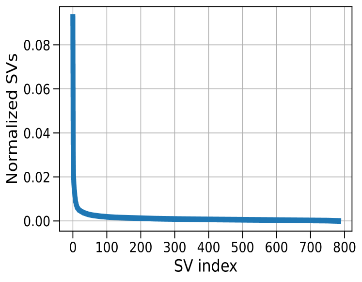
(a) MNIST-Linear scale

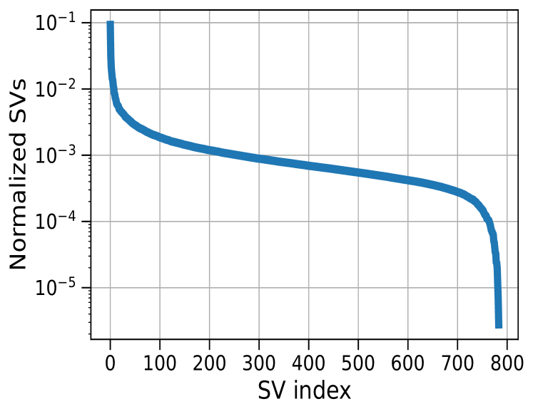
(b) MNIST-Log scale

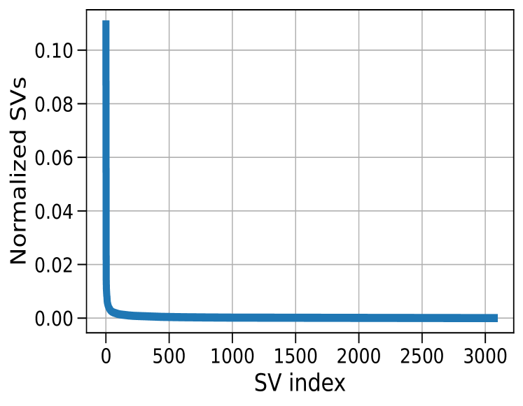
(c) CIFAR-10-Linear scale

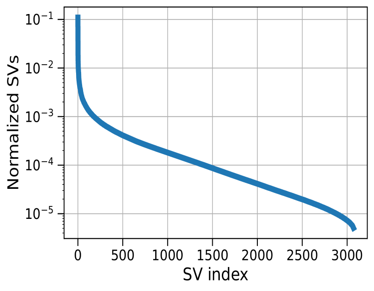
(d) CIFAR-10-Log scale

Figure 7: The values of normalized singular values of the data matrix for the MNIST and CIFAR-10 datasets. As illustrated in both figures, the singular values follow an exponentially decaying trends indicating an effective low rank structure.

A.10 Proof of Proposition 2 and Corollary 1

We first review the multi-layer hyperplane arrangements concept introduced in Section 2.1 of [21]. Based on this concept, we then calculate the training complexity to globally solve the convex program in Theorem 1.

If we denote the number of hyperplane arrangements for the first ReLU layer as $P_{1}$, then from Appendix A.8 we know that

$$P_{1}\leq 2r\left(\frac{e(n-1)}{r}\right)^{r}\approx\mathcal{O}(n^{r}).$$ (24)

In order to obtain a bound for the number of hyperplane arrangements in the second ReLU layer we first note that preactivations of the second ReLU layer, i.e., $\left({\bf X}\mathbf{W}_{1}\right)_{+}\mathbf{w}_{2}$ can be equivalently represented as a matrix-vector product form by using the effective data matrix $\bar{{\bf X}}:=\begin{bmatrix}\mathcal{I}_{1}\mathbf{D}_{11}{\bf X}&\mathcal{I}_{2}\mathbf{D}_{12}{\bf X}&\ldots&\mathcal{I}_{m_{1}}\mathbf{D}_{1m_{1}}{\bf X}\end{bmatrix}$ due to the equivalent representation in (3). Therefore, given $\mathrm{rank}(\bar{{\bf X}})=r_{2}\leq m_{1}r$

$$\bar{P}_{2}\leq 2\sum_{k=0}^{r_{2}-1}{n-1\choose k}\leq 2r_{2}\left(\frac{e(n-1)}{r_{2}}\right)^{r_{2}}\leq 2m_{1}r\left(\frac{e(n-1)}{m_{1}r}\right)^{m_{1}r}.$$

However, notice that $\bar{{\bf X}}$ is not a fixed data matrix since we can choose each diagonal $\mathbf{D}_{1j_{1}}$ among a set $\{\mathbf{D}_{i}\}_{i=1}^{P_{1}}$ of size $P_{1}$ due to (24) and the sign pattern $\mathcal{I}_{j_{1}}$ among the set $\{+1,-1\}$ of size $2$. Thus, in the worst-case, we have the following upper-bound

$$P_{2}\leq\bar{P}_{2}(2P_{1})^{m_{1}}\leq\frac{2^{2m_{1}+1}(e(n-1))^{2m_{1}r}}{m_{1}^{m_{1}r-1}r^{2m_{1}r-m_{1}-1}}\approx\mathcal{O}(n^{m_{1}r}).$$ (25)

Notice that given fixed scalars $m_{1}$ and $r$, both $P_{1}$ and $P_{2}$ are polynomial terms with respect to the number of data samples $n$ and the feature dimension $d$.

Remark 3.

Notice that Convolutional Neural Networks (CNNs) operate on the patch matrices $\{{\bf X}_{b}\}_{b=1}^{B}$ instead of the full data matrix ${\bf X}$, where ${\bf X}_{b}\in\mathbb{R}^{n\times h}$ and $h$ denotes the filter size. Hence, even when the data matrix is full rank, i.e., $r=\min\{n,d\}$, the number of hyperplane arrangements $P_{1}$ is upperbounded as $P_{1}\leq\mathcal{O}(n^{r_{c}})$, where $r_{c}:=\max_{b}\mbox{rank}({\bf X}_{b})\leq h\ll\min\{n,d\}$ (see [45] for details). For instance, let us consider a CNN with $m_{1}=512$ filters of size $3\times 3$, then $r_{c}\leq 9$ independent of data dimension $n,d$. As a consequence, weight sharing structure in CNNs dramatically limits the number of possible hyperplane arrangements. This also explains efficiency and remarkable generalization performance of CNNs in practice.

Training complexity analysis: Here, we calculate the computational complexity to globally solve the convex program in (8). Note that (8) is a convex optimization problem with $2dm_{1}MP_{1}P_{2}$ variables and $2n(m_{1}+1)MP_{1}P_{2}$ constraints. Therefore, due to the upperbounds in (24) and (25) of Appendix A.8, the convex program (8) can be globally optimized by a standard interior-point solver with the computational complexity $\mathcal{O}(d^{3}m_{1}^{3}2^{3(m_{1}+1)}n^{3(m_{1}+1)r})$, which is a polynomial-time complexity in terms of $n,d$.

The analysis in this section can be recursively extended to arbitrarily deep parallel networks. First notice that if we apply the same approach to obtain an upperbound on $P_{3}$, then due to the multiplicative pattern in (25), we obtain $P_{3}\leq P_{3}^{\prime}(2P_{2})^{m_{2}}\leq\mathcal{O}(n^{m_{2}m_{1}r})$. In a similar manner, the number of hyperplane arrangements in the $l^{th}$ layer is upperbounded as $P_{l}\leq\mathcal{O}(n^{r\prod_{j=1}^{l-1}m_{j}})$, which is polynomial in both $n$ and $d$ for fixed data rank $r$ and fixed layer widths $\{m_{j}\}_{j=1}^{l-1}$.

∎

A.11 Extension to vector outputs

In this section, we extend the analysis to parallel networks with multiple outputs where the label matrix is defined as $\mathbf{Y}\in\mathbb{R}^{n\times C}$ provided that there exist $C$ classes/outputs. Then the primal non-convex training problem is as follows

$$p_{v}^{*}:= \min_{\theta\in\Theta}\mathcal{L}\left(\sum_{k=1}^{K}f_{\theta,k}({\bf X}),\mathbf{Y}\right)+\beta\sum_{k=1}^{K}\sqrt{\sum_{j_{1},j_{2},\ldots,j_{L}}\left(\|\mathbf{w}_{1kj_{1}}\|_{2}^{2}\prod_{l=2}^{L-1}w_{lkj_{l-1}j_{l}}^{2}\|\mathbf{w}_{Lkj_{L-1}j_{L}}^{2}\|^{2}\right)}.$$

Applying Lemma 1 and each step in the proof of Theorem 1 yield

$$d_{v}^{*}:=\max_{\mathbf{\mathbf{V}}}\min_{\begin{subarray}{c}\theta\in\Theta_{s}\end{subarray}}-\mathcal{L}^{*}(\mathbf{V})\text{ s.t. }\left\|\mathbf{V}^{T}\left(\left({\bf X}\mathbf{W}_{1k}\right)_{+}\ldots\mathbf{W}_{(L-1)k}\right)_{+}\right\|_{F}\leq\beta,\,\forall k\in[K],$$

where the corresponding Fenchel conjugate function is

$$\mathcal{L}^{*}(\mathbf{V}):=\max_{\mathbf{Z}}\mathrm{trace}\left(\mathbf{Z}^{T}\mathbf{V}\right)-\mathcal{L}\left(\mathbf{Z},\mathbf{Y}\right)\,.$$

Notice that above we have a dual matrix $\mathbf{V}$ instead of the dual vector in the scalar output case. More importantly, here, we have $\ell_{2}$ norm in the dual constraint unlike the scalar output case with absolute value. Therefore, the vector-output case is slightly more challenging than the scalar output case and yields a different regularization function in the equivalent convex program.

The rest of the derivations directly follows the steps in Section A.4 and [62].

References

- [1] Behnam Neyshabur, Ryota Tomioka, and Nathan Srebro. Norm-based capacity control in neural networks. In Peter Grünwald, Elad Hazan, and Satyen Kale, editors, Proceedings of The 28th Conference on Learning Theory, volume 40 of Proceedings of Machine Learning Research, pages 1376–1401, Paris, France, 03–06 Jul 2015. PMLR.
- [2] Behnam Neyshabur, Russ R Salakhutdinov, and Nati Srebro. Path-sgd: Path-normalized optimization in deep neural networks. In C. Cortes, N. Lawrence, D. Lee, M. Sugiyama, and R. Garnett, editors, Advances in Neural Information Processing Systems, volume 28. Curran Associates, Inc., 2015.
- [3] Tolga Ergen and Mert Pilanci. Convex geometry of two-layer relu networks: Implicit autoencoding and interpretable models. In Silvia Chiappa and Roberto Calandra, editors, Proceedings of the Twenty Third International Conference on Artificial Intelligence and Statistics, volume 108 of Proceedings of Machine Learning Research, pages 4024–4033, Online, 26–28 Aug 2020. PMLR.
- [4] Tolga Ergen and Mert Pilanci. Convex geometry and duality of over-parameterized neural networks. Journal of Machine Learning Research, 22(212):1–63, 2021.
- [5] T. Ergen and M. Pilanci. Convex optimization for shallow neural networks. In 2019 57th Annual Allerton Conference on Communication, Control, and Computing (Allerton), pages 79–83, 2019.
- [6] Mert Pilanci and Tolga Ergen. Neural networks are convex regularizers: Exact polynomial-time convex optimization formulations for two-layer networks. In Hal Daumé III and Aarti Singh, editors, Proceedings of the 37th International Conference on Machine Learning, volume 119 of Proceedings of Machine Learning Research, pages 7695–7705. PMLR, 13–18 Jul 2020.
- [7] Shai Shalev-Shwartz, Ohad Shamir, and Shaked Shammah. Failures of gradient-based deep learning. arXiv preprint arXiv:1703.07950, 2017.
- [8] Ian Goodfellow, Yoshua Bengio, Aaron Courville, and Yoshua Bengio. Deep learning, volume 1. MIT press Cambridge, 2016.
- [9] Rong Ge, Jason D. Lee, and Tengyu Ma. Learning one-hidden-layer neural networks with landscape design, 2017.
- [10] Itay Safran and Ohad Shamir. Spurious local minima are common in two-layer relu neural networks. In International Conference on Machine Learning, pages 4433–4441. PMLR, 2018.
- [11] Animashree Anandkumar and Rong Ge. Efficient approaches for escaping higher order saddle points in non-convex optimization. In Conference on learning theory, pages 81–102, 2016.
- [12] Bhaskar DasGupta, Hava T Siegelmann, and Eduardo Sontag. On the complexity of training neural networks with continuous activation functions. IEEE Transactions on Neural Networks, 6(6):1490–1504, 1995.
- [13] Avrim Blum and Ronald L Rivest. Training a 3-node neural network is np-complete. In Advances in neural information processing systems, pages 494–501, 1989.
- [14] Peter Bartlett and Shai Ben-David. Hardness results for neural network approximation problems. In European Conference on Computational Learning Theory, pages 50–62. Springer, 1999.
- [15] Alon Brutzkus, Amir Globerson, Eran Malach, and Shai Shalev-Shwartz. SGD learns over-parameterized networks that provably generalize on linearly separable data. CoRR, abs/1710.10174, 2017.
- [16] Simon S Du and Jason D Lee. On the power of over-parametrization in neural networks with quadratic activation. arXiv preprint arXiv:1803.01206, 2018.
- [17] Sanjeev Arora, Nadav Cohen, and Elad Hazan. On the optimization of deep networks: Implicit acceleration by overparameterization. In 35th International Conference on Machine Learning, ICML 2018, pages 372–389. International Machine Learning Society (IMLS), 2018.
- [18] Behnam Neyshabur, Zhiyuan Li, Srinadh Bhojanapalli, Yann LeCun, and Nathan Srebro. Towards understanding the role of over-parametrization in generalization of neural networks. arXiv preprint arXiv:1805.12076, 2018.
- [19] Yifei Wang, Tolga Ergen, and Mert Pilanci. Parallel deep neural networks have zero duality gap. In The Eleventh International Conference on Learning Representations, 2023.
- [20] Tolga Ergen and Mert Pilanci. Revealing the structure of deep neural networks via convex duality. In Marina Meila and Tong Zhang, editors, Proceedings of the 38th International Conference on Machine Learning, volume 139 of Proceedings of Machine Learning Research, pages 3004–3014. PMLR, 18–24 Jul 2021.
- [21] Tolga Ergen and Mert Pilanci. Global optimality beyond two layers: Training deep relu networks via convex programs. In Marina Meila and Tong Zhang, editors, Proceedings of the 38th International Conference on Machine Learning, volume 139 of Proceedings of Machine Learning Research, pages 2993–3003. PMLR, 18–24 Jul 2021.
- [22] Hongyang Zhang, Junru Shao, and Ruslan Salakhutdinov. Deep neural networks with multi-branch architectures are intrinsically less non-convex. In The 22nd International Conference on Artificial Intelligence and Statistics, pages 1099–1109, 2019.
- [23] Benjamin D Haeffele and René Vidal. Global optimality in neural network training. In Proceedings of the IEEE Conference on Computer Vision and Pattern Recognition, pages 7331–7339, 2017.
- [24] Sergey Zagoruyko and Nikos Komodakis. Wide residual networks. arXiv preprint arXiv:1605.07146, 2016.
- [25] Andreas Veit, Michael J Wilber, and Serge Belongie. Residual networks behave like ensembles of relatively shallow networks. In Advances in neural information processing systems, pages 550–558, 2016.
- [26] Forrest N Iandola, Song Han, Matthew W Moskewicz, Khalid Ashraf, William J Dally, and Kurt Keutzer. Squeezenet: Alexnet-level accuracy with 50x fewer parameters and< 0.5 mb model size. arXiv preprint arXiv:1602.07360, 2016.
- [27] Christian Szegedy, Sergey Ioffe, Vincent Vanhoucke, and Alexander A Alemi. Inception-v4, inception-resnet and the impact of residual connections on learning. In Thirty-first AAAI conference on artificial intelligence, 2017.
- [28] François Chollet. Xception: Deep learning with depthwise separable convolutions. In Proceedings of the IEEE conference on computer vision and pattern recognition, pages 1251–1258, 2017.
- [29] Saining Xie, Ross Girshick, Piotr Dollár, Zhuowen Tu, and Kaiming He. Aggregated residual transformations for deep neural networks. In Proceedings of the IEEE conference on computer vision and pattern recognition, pages 1492–1500, 2017.
- [30] Raman Arora, Amitabh Basu, Poorya Mianjy, and Anirbit Mukherjee. Understanding deep neural networks with rectified linear units. In 6th International Conference on Learning Representations, ICLR 2018, 2018.
- [31] Surbhi Goel, Adam Klivans, Pasin Manurangsi, and Daniel Reichman. Tight Hardness Results for Training Depth-2 ReLU Networks. In James R. Lee, editor, 12th Innovations in Theoretical Computer Science Conference (ITCS 2021), volume 185 of Leibniz International Proceedings in Informatics (LIPIcs), pages 22:1–22:14, Dagstuhl, Germany, 2021. Schloss Dagstuhl–Leibniz-Zentrum für Informatik.
- [32] Vincent Froese, Christoph Hertrich, and Rolf Niedermeier. The computational complexity of relu network training parameterized by data dimensionality, 2021.
- [33] Kaiming He, Xiangyu Zhang, Shaoqing Ren, and Jian Sun. Deep residual learning for image recognition. In Proceedings of the IEEE conference on computer vision and pattern recognition, pages 770–778, 2016.
- [34] Zhen Dai, Mina Karzand, and Nathan Srebro. Representation costs of linear neural networks: Analysis and design. In M. Ranzato, A. Beygelzimer, Y. Dauphin, P.S. Liang, and J. Wortman Vaughan, editors, Advances in Neural Information Processing Systems, volume 34, pages 26884–26896. Curran Associates, Inc., 2021.
- [35] Saharon Rosset, Grzegorz Swirszcz, Nathan Srebro, and Ji Zhu. L1 regularization in infinite dimensional feature spaces. In International Conference on Computational Learning Theory, pages 544–558. Springer, 2007.
- [36] Stephen Boyd and Lieven Vandenberghe. Convex optimization. Cambridge university press, 2004.
- [37] Tolga Ergen and Mert Pilanci. Convex geometry and duality of over-parameterized neural networks. Journal of Machine Learning Research, 22(212):1–63, 2021.
- [38] Francis Bach. Breaking the curse of dimensionality with convex neural networks. The Journal of Machine Learning Research, 18(1):629–681, 2017.
- [39] Zeyuan Allen-Zhu, Yuanzhi Li, and Yingyu Liang. Learning and generalization in overparameterized neural networks, going beyond two layers. In H. Wallach, H. Larochelle, A. Beygelzimer, F. d'Alché-Buc, E. Fox, and R. Garnett, editors, Advances in Neural Information Processing Systems, volume 32. Curran Associates, Inc., 2019.
- [40] Huy Tuan Pham and Phan-Minh Nguyen. Global convergence of three-layer neural networks in the mean field regime. In International Conference on Learning Representations, 2021.
- [41] Eugene Belilovsky, Michael Eickenberg, and Edouard Oyallon. Greedy layerwise learning can scale to imagenet. In International conference on machine learning, pages 583–593. PMLR, 2019.
- [42] Alex Krizhevsky, Vinod Nair, and Geoffrey Hinton. The CIFAR-10 dataset. http://www.cs.toronto.edu/kriz/cifar.html, 2014.
- [43] Han Xiao, Kashif Rasul, and Roland Vollgraf. Fashion-mnist: a novel image dataset for benchmarking machine learning algorithms, 2017.
- [44] Tolga Ergen, Halil I. Gulluk, Jonathan Lacotte, and Mert Pilanci. Globally optimal training of neural networks with threshold activation functions. In The Eleventh International Conference on Learning Representations, 2023.
- [45] Tolga Ergen and Mert Pilanci. Implicit convex regularizers of cnn architectures: Convex optimization of two- and three-layer networks in polynomial time. In International Conference on Learning Representations, 2021.
- [46] Arda Sahiner, Tolga Ergen, Batu Ozturkler, Burak Bartan, John M. Pauly, Morteza Mardani, and Mert Pilanci. Hidden convexity of wasserstein GANs: Interpretable generative models with closed-form solutions. In International Conference on Learning Representations, 2022.
- [47] Tolga Ergen, Arda Sahiner, Batu Ozturkler, John M. Pauly, Morteza Mardani, and Mert Pilanci. Demystifying batch normalization in reLU networks: Equivalent convex optimization models and implicit regularization. In International Conference on Learning Representations, 2022.
- [48] Vikul Gupta, Burak Bartan, Tolga Ergen, and Mert Pilanci. Convex neural autoregressive models: Towards tractable, expressive, and theoretically-backed models for sequential forecasting and generation. In ICASSP 2021 - 2021 IEEE International Conference on Acoustics, Speech and Signal Processing (ICASSP), pages 3890–3894, 2021.
- [49] Tolga Ergen, Behnam Neyshabur, and Harsh Mehta. Convexifying transformers: Improving optimization and understanding of transformer networks. arXiv, 2022.
- [50] Arda Sahiner, Tolga Ergen, Batu Ozturkler, John Pauly, Morteza Mardani, and Mert Pilanci. Unraveling attention via convex duality: Analysis and interpretations of vision transformers. In Kamalika Chaudhuri, Stefanie Jegelka, Le Song, Csaba Szepesvari, Gang Niu, and Sivan Sabato, editors, Proceedings of the 39th International Conference on Machine Learning, volume 162 of Proceedings of Machine Learning Research, pages 19050–19088. PMLR, 17–23 Jul 2022.
- [51] Daniel Smilkov Carter and Shan. A neural network playground. https://playground.tensorflow.org/.
- [52] Michael Grant and Stephen Boyd. CVX: Matlab software for disciplined convex programming, version 2.1. http://cvxr.com/cvx, March 2014.
- [53] Steven Diamond and Stephen Boyd. CVXPY: A Python-embedded modeling language for convex optimization. Journal of Machine Learning Research, 17(83):1–5, 2016.
- [54] Akshay Agrawal, Robin Verschueren, Steven Diamond, and Stephen Boyd. A rewriting system for convex optimization problems. Journal of Control and Decision, 5(1):42–60, 2018.
- [55] Dheeru Dua and Casey Graff. UCI machine learning repository, 2017.
- [56] Manuel Fernández-Delgado, Eva Cernadas, Senén Barro, and Dinani Amorim. Do we need hundreds of classifiers to solve real world classification problems? Journal of Machine Learning Research, 15(90):3133–3181, 2014.
- [57] Maurice Sion. On general minimax theorems. Pacific J. Math., 8(1):171–176, 1958.
- [58] Piyush C Ojha. Enumeration of linear threshold functions from the lattice of hyperplane intersections. IEEE Transactions on Neural Networks, 11(4):839–850, 2000.
- [59] Richard P Stanley et al. An introduction to hyperplane arrangements. Geometric combinatorics, 13:389–496, 2004.
- [60] RO Winder. Partitions of n-space by hyperplanes. SIAM Journal on Applied Mathematics, 14(4):811–818, 1966.
- [61] Thomas M Cover. Geometrical and statistical properties of systems of linear inequalities with applications in pattern recognition. IEEE transactions on electronic computers, (3):326–334, 1965.
- [62] Arda Sahiner, Tolga Ergen, John M. Pauly, and Mert Pilanci. Vector-output relu neural network problems are copositive programs: Convex analysis of two layer networks and polynomial-time algorithms. In International Conference on Learning Representations, 2021.