TESS Hunt for Young and Maturing Exoplanets (THYME) VI: an 11 Myr Giant Planet Transiting a Very Low Mass Star in Lower Centaurus Crux

Abstract

Mature super-Earths and sub-Neptunes are predicted to be $\simeq$Jovian radius when younger than $10$ Myr. Thus, we expect to find 5–15$R_{\oplus}$ planets around young stars even if their older counterparts harbor none. We report the discovery and validation of TOI 1227 b, a $0.85\pm 0.05\,R_{J}$ (9.5$R_{\oplus}$) planet transiting a very low-mass star ($0.170\pm 0.015\,M_{\odot}$) every 27.4 days. TOI 1227’s kinematics and strong lithium absorption confirm it is a member of a previously discovered sub-group in the Lower Centaurus Crux OB association, which we designate the Musca group. We derive an age of 11$\pm$2 Myr for Musca, based on lithium, rotation, and the color-magnitude diagram of Musca members. The TESS data and ground-based follow-up show a deep (2.5%) transit. We use multiwavelength transit observations and radial velocities from the IGRINS spectrograph to validate the signal as planetary in nature, and we obtain an upper limit on the planet mass of $\simeq$0.5 $M_{J}$. Because such large planets are exceptionally rare around mature low-mass stars, we suggest that TOI 1227 b is still contracting and will eventually turn into one of the more common $<5R_{\oplus}$ planets.

2022 March 9

1 Introduction

Young planets offer a window into the early stages of planet formation and evolution. Planets younger than 100 Myr are particularly useful for this work, as planetary systems likely evolve most rapidly in the first few hundred million years after formation (Lopez & Fortney, 2013; Owen & Wu, 2013). Populations of such planets are critical to understanding planetary migration (Nelson et al., 2017), photoevaporation (Raymond et al., 2008; Owen & Lai, 2018), and atmospheric chemistry (e.g., Segura et al., 2005; Gao & Zhang, 2020). Given the timescale for planet formation (1-10 Myr; Yin et al., 2002; Alibert et al., 2005), planets aged $\lesssim$30 Myr can even tell us about the conditions of planets right after their formation.

The number of known young transiting planets has grown significantly in recent years (e.g., Obermeier et al., 2016; David et al., 2018; Benatti et al., 2019; Newton et al., 2021). This growth was primarily driven by a combination of the K2 and TESS missions surveying nearby young clusters and star-forming regions (Ricker et al., 2014; Van Cleve et al., 2016), improvements in filtering variability in young stars (e.g., Aigrain et al., 2016; Rizzuto et al., 2017), and more complete identification of young stellar associations from Gaia kinematics (e.g., Cantat-Gaudin et al., 2018; Kerr et al., 2021). Despite this progress, there are still only a handful of transiting planets at the youngest ages of $\lesssim$30 Myr (David et al., 2016; Mann et al., 2016a; David et al., 2019a; Plavchan et al., 2020; Rizzuto et al., 2020) and a few candidate nontransiting planets from radial velocity surveys (e.g., Johns-Krull et al., 2016; Donati et al., 2017).

Models predict that gas giant planets younger than $<50$ Myr will be larger and brighter than their older counterparts (Linder et al., 2019). At 10–20 Myr, progenitors of mature Jovian-mass planets are expected to be 1.2–1.6 $R_{J}$ and sub-Neptunes $\sim 1R_{J}$ (Linder et al., 2019; Owen, 2020). Completeness curves from the best search pipelines (Rizzuto et al., 2017), and the discovery of much smaller planets (e.g., Mann et al., 2018; Zhou et al., 2020) demonstrate that giant planets are readily detectable even in the presence of complex stellar variability common to young stars. Thus far, transit surveys of young stars identified only a few Jovian-radius planets in the youngest associations (David et al., 2019b; Bouma et al., 2020; Rizzuto et al., 2020).

As part of the TESS Hunt for Young and Maturing Exoplanets survey (THYME; Newton et al., 2019), our team searches TESS data using a specialized pipeline to identify young planets missed by standard searches (e.g., Rizzuto et al., 2020), and checks previously-identified planet candidates for signs of membership in a young association (e.g., Mann et al., 2020; Newton et al., 2021). We identified TOI 1227 (2MASS J12270432-7227064, TIC 360156606) as a member of a young association, with a planet candidate (TOI1227.01) identified by the TESS mission, and astrometry consistent with membership in the Lower Centaurus Crux (LCC) region of the Scorpius-Centaurus (Sco-Cen) OB association (Goldman et al., 2018; Damiani et al., 2019). The TESS-identified transit signal is $\simeq$2% deep, suggesting a Jovian-sized planet orbiting a pre-main-sequence low-mass star. As giant planets with periods $<$100 days are rare around older stars of similar mass ($<1\%$ Bonfils et al., 2013), validation of this planet would provide strong evidence of radius evolution.

In this work, we present validation, characterization, and age estimates for TOI 1227 b, a 0.85$R_{Jup}$ planet orbiting a $\simeq$11 Myr pre-main-sequence M5V star (0.17$M_{\odot}$) every 27.26 days. In Section 2, we detail the photometric and spectroscopic follow-up of the planet and host star. We demonstrate that the star is a member of a recently identified substructure of LCC and derive an updated age of $11\pm 2$ Myr for the parent population in Section 3. We estimate parameters for the host star in Section 4, parameters of the planet in Section 5, and combine these with our ground-based follow-up to statistically validate the planet in Section 6. We place the large size of TOI 1227 b in context with its age and host star mass and explore its likely evolution in Section 7. We conclude in Section 8 with a summary and discussion of follow-up and implications for future searches for young exoplanets.

2 Observations

2.1 TESS Photometry

TOI 1227 was observed by the TESS mission (Ricker et al., 2014) from UT 22 Apr 2019 through 19 Jun 2019 (Sectors 11 and 12) and then again from 28 Apr 2021 through 26 May 2021 (Sector 38). In all three sectors, the target fell on Camera 3. The first two sectors had 2 min cadence data as part of a search for planets around M dwarfs (G011180; PI Dressing). Sector 38 had 20 s cadence data, as it was known to be a young TOI at that phase (G03141; PI Newton). We initially used the 2 min cadence for all analysis for computational efficiency and TESS cosmic-ray mitigation (not included in 20 s data), but also ran a separate analysis using the Sector 38 20 s data (see Section 5. In both cases, we used the Pre-Search Data Conditioning Simple Aperture Photometry (PDCSAP; Stumpe et al., 2012; Smith et al., 2012; Stumpe et al., 2014) TESS light curve produced by the Science Process Operations center (SPOC; Jenkins et al., 2016) and available through the Mikulski Archive for Space Telescopes (MAST).

2.2 Identification of the transit signal

The planet signal, TOI1227.01, was first detected in a joint transit search of sectors 11 and 12 (one transit in each) with an adaptive wavelet-based detector (Jenkins, 2002; Jenkins et al., 2010). The candidate was fitted with a limb-darkened light curve (Li et al., 2019) and passed all performed diagnostic tests (Twicken et al., 2018). Although the difference image centroiding failed to converge, the difference images indicate that the transit source location was consistent with the location of the host star, TOI 1227. A search of the residual light curve failed to identify additional transiting planet signatures. The TESS Science Office reviewed the diagnostic test results and issued an alert for this planet candidate as a TESS object of interest (TOI) on 2019 August 26 (Guerrero et al., 2021). A third transit was detected in the Sector 38 TESS data, consistent with the expected period and depth.

We searched for additional planets using the Notch and LoCoR pipelines, as described in Rizzuto et al. (2017). This included using the significance of adding a trapezoidal Notch to the light curve detrending, as characterized by the Bayesian information criterion (BIC). The method was more effective than periodic methods for finding planets with $\lesssim$3 transits, as was the case for HIP 67522 b (Rizzuto et al., 2020). The transits were quite clear from the BIC test. However, no additional significant signals were detected.

TOI 1227 is a relatively faint star ($T=13.8$) in a crowded region (see Figure 1). Within 2′ ($\simeq$6 TESS pixels), there are four sources brighter than TOI 1227, one of which is $T=8.4$ (TIC 360156594). Two sources brighter than TOI 1227 are within 1′. While the TESS aperture was small (4–6 pixels over the 3 sectors), background contamination was likely to be a problem for the TESS data. Correcting for contamination and confirming the planet were the major motivations for our ground-based follow-up.

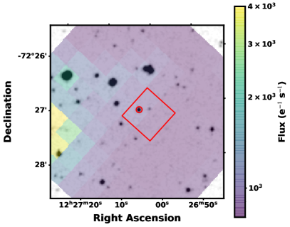
Figure 1: A TESS Sector 11 image colored by flux (see colorbar) on top of a DSS image (greyscale). The red circle indicates TOI 1227 and the red box indicates the TESS aperture used for Sector 11 (the aperture varied between sectors). The TESS PSF in this region has a full-width half-max of approximately 1.9 TESS pixels. The large TESS PSF combined with a faint source meant that there were high levels of contamination around TOI 1227.

2.3 Ground-Based Photometry

The photometry is summarized in Table 1. We provide details by instrument below.

Table 1: Log of transit observations

Start	Telescope	Filter	Transit #	Texp	Obs Duration
(UT)			#	(s)	(h)
2019 Apr 22	TESS S11	TESS	1	120	N/A
2019 Apr 22	TESS S12	TESS	2	120	N/A
2020 Jan 15	SOAR	$i$’	9	120	8.1
2020 Jan 15	LCO	$i$’	9	200	2.8
2020 May 03	LCO	$i$’	13	200	1.9
2020 Jul 24	LCO	$r$’	16	200	2.5
2020 Jul 24	LCO	$z_{s}$	16	200	2.5
2021 Mar 28	SOAR	$g$’	25	120	7.6
2021 Apr 24	ASTEP	$Rc$’	26	200	5.7
2021 Apr 24	LCO	$g$’	26	300	6.2
2021 Apr 24	LCO	$z_{s}$	26	210	6.2
2021 Apr 28	TESS S38	TESS	27	20	N/A
2021 Jun 17	LCO	$g$’	28	300	4.1

2.3.1 Goodman/SOAR

We observed two transits of TOI 1227 b using the SOAR 4.1 m telescope at Cerro Pachón, Chile, with the Goodman High Throughput Spectrograph in imaging mode (Clemens et al., 2004). For both observations, we used the red camera. In this mode, Goodman has a default 7.2′ diameter circular field of view with a pixel scale of 0.15″ pixel^-1. The first transit was observed on 2020 Jan 15 with the SDSS $i$’ filter, and the second transit was observed on 2021 Mar 28 with the SDSS $g$’ filter. Both nights had photometric conditions for the full duration of the transit observations. Although TOI 1227 is much fainter in $g$’ than in $i$’, we used a 120 s exposure time for both filters to resolve any flares and sample the ingress. We selected a smaller region-of-interest in the readout direction (1598 pixels) to decrease readout time to 1.7 s. Due to the small pixel scale, no defocusing was required and counts were well below half-well depth for both the target and all but one target in the field of view (HD 108342).

About 1 hour into the 2021 Mar 28 transit observations, the SOAR guider began to fail, causing the target to shift $\simeq$5 pixels per exposure and forcing us to shift it back manually every $\sim$10 exposures. During egress, the guider completely failed and had to be reset before re-acquiring the field. We positioned the target back to its starting location and continued the observations as normal. This resulted in poorer photometric precision than normally achievable with Goodman/SOAR, and a $\simeq$15 min gap in the data near the end of the egress.

We applied bias and flat-field corrections before extracting photometry for TOI 1227 using a 10-pixel radius aperture and used an annulus of 30–60 pixels to determine the local sky background. The aperture center for each exposure was the stellar centroid, calculated within a 10-pixel radius of the nominal location. We repeated this on eight nearby stars that were close in brightness to the target and showed little or no photometric variation when compared to other stars in the field. We corrected the target light curve using the weighted mean of the comparison star curves.

2.3.2 LCO Photometry

We observed a total of seven transits with 1 m telescopes in the Las Cumbres Observatory network (LCO ; Brown et al., 2013). These were all observed with Sinistro cameras, with a pixel scale of 0.389″ pixel^-1. Two transits were observed using the SDSS $g^{\prime}$ filter, one with SDSS $r^{\prime}$, two with $i^{\prime}$, and two with $z_{s}$. Exposure times are given in Table 1. Because of the difficulty of scheduling observations of a long-period planet ($\sim$27 d) and weather interruptions, all LCO observations covered only part of the transit.

The images were initially calibrated by the standard LCOGT BANZAI pipeline (McCully et al., 2018). We then performed aperture photometry on all datasets using the AstroImageJ package (AIJ; Collins et al., 2017). The aperture varied based on the seeing conditions at the observatory, but we generally used a 6–10 pixel radius circular aperture for the source and an annulus with a 15–20 pixel inner radius and a 25–30 pixel outer radius for the sky background. For all observations, we centered the apertures on the source and weighted pixels within the aperture equally. Because the event was detected on the source, the usual check of nearby sources for evidence of an eclipsing binary was not necessary. Light curves of nearby sources are available with the extracted light curves and further details on the follow-up at ExoFOP-TESS (ExoFOP, 2019).

Except for a 2021 Apr 24 $g$’ transit, all photometry showed the expected transit behavior. Two transits had poor coverage (no out-of-transit baseline), but still showed a shape consistent with ingress. We discuss the 2021 Apr 24 transit in more detail in Section 6.4.

2.3.3 ASTEP Photometry

On UTC 2021 Apr 24, one additional transit was observed with the Antarctica Search for Transiting ExoPlanets (ASTEP) program on the East Antarctic plateau (Guillot et al., 2015; Mékarnia et al., 2016). The 0.4 m telescope is equipped with an FLI Proline science camera with a KAF-16801E, $4096\times 4096$ front-illuminated CCD. The camera has an image scale of 0.93″ pixel^-1 resulting in a 1${}^{o}\times 1^{o}$ corrected field of view. The focal instrument dichroic plate splits the beam into a blue wavelength channel for guiding, and a non-filtered red science channel roughly matches an $R_{c}$ transmission curve.

Due to the extremely low data transmission rate at the Concordia Station, the data are processed on-site using an automated IDL-based pipeline described in Abe et al. (2013). The calibrated light curve is reported via email and the raw light curves of about 1,000 stars are transferred to Europe on a server in Rome, Italy, and are then available for deeper analysis. These data files contain each star’s flux computed through $10$ fixed circular aperture radii so that optimal light curves can be extracted. For TOI 1227, a 9.3-pixel radius aperture gave the best result.

TOI 1227 was observed under mixed conditions, with a windy clear sky, and air temperatures between $-62^{o}$C and $-66^{o}$C. The Moon was $\sim 90\%$ full and present during the observation. A strong wind ($\sim$ 6 ms^-1) led to telescope guiding issues at the beginning of the observation and prevented us from observing the ingress. The data points corresponding to these issues were removed from the analysis. However, the resulting light curve showed the expected egress.

2.4 Corrections for second-order extinction

Since atmospheric extinction is strongly color-dependent, changes in airmass produce color-dependent flux losses that depend on the spectral energy distribution (SED) of the target. These color terms are weaker in redder and narrower passbands (Young et al., 1991). The effect is often small, as comparison stars typically span a range of colors, and observations are timed for favorable airmass. However, TOI 1227 was unusual both because of its long orbital period (27.3 d) and red color; of stars $<$5′ from the target and differing by $<$1 magnitude in $G$, the reddest has a Gaia color of $BP-RP=2.1$ while TOI 1227 has $BP-RP=3.3$.

Because we had few options for mitigating second-order extinction (color terms), we corrected for the effect following Mann et al. (2011). To summarize, we estimated $T_{\text{eff}}$ for all comparison stars based on their Gaia colors and the tables from Pecaut & Mamajek (2013). We then combined the relevant BT-SETTL models (assuming Solar metallicity) with an airmass-dependent model of the atmosphere above the observing site (Rothman et al., 2009) and the appropriate filter profile. The output was a predicted change in flux from second-order extinction alone. The trend was negligible ($<1$ mmag) for $i$’ and $z_{s}$ observations, so we did not apply a correction. The effect was small but non-negligible for $r$ ($>$1 mmag), and significant for $g$’-band observations (as large as 5 mmag), so we applied it to those datasets.

2.5 Spectroscopy

2.5.1 Goodman/SOAR

We observed TOI 1227 with the Goodman spectrograph (Clemens et al., 2004) on the Southern Astrophysical Research (SOAR) 4.1 m telescope located at Cerro Pachón, Chile, on two nights. We used the red camera, the 1200 l/mm grating in the M5 setup, and the 0.46″ slit rotated to the parallactic angle. This setup gave a resolution of $R\simeq$ 5880 spanning 6150–7500Å.

We obtained the first spectrum on 2019 Dec 12 (UT) shortly after the target was alerted as a TOI, to check for signs of youth. We obtained three back-to-back exposures of TOI 1227, each with an exposure time of 800 s. The resulting spectrum showed the Li and H$\alpha$ expected for a young star and TiO features consistent with an M5 dwarf, as we show in Figure 2. Once we confirmed the planetary signal (based on ground-based transits), we obtained an additional spectrum on 2021 Feb 23 (UT) under clear conditions. Our goal was a spectrum with a signal-to-noise ratio (SNR) $\gg$100 per pixel across the full wavelength range, to use for stellar characterization (Section 4). To this end, we used an exposure time of 1800 s for five back-to-back exposures.

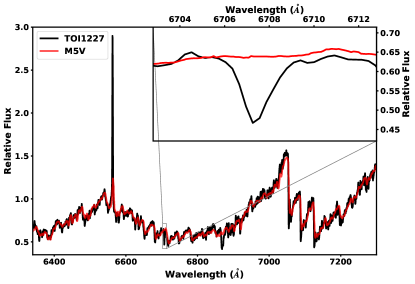
Figure 2: Goodman spectrum of TOI 1227 (black) and a template M5V dwarf from Kesseli et al. (2017). Because of extinction around TOI 1227 and imperfect flux calibration from Goodman, we fit out a 2nd-order polynomial on the Goodman spectrum to better match the template. The Goodman spectrum is also higher resolution than the template ($R$ of 5880 vs 2000). The inset highlights the Li 6708Å line, which is absent in the spectrum of older stars like the template, but strong in TOI 1227’s spectrum.

To better determine the age of TOI 1227, we also observed 13 nearby stars that are likely part of the same grouping in LCC as TOI 1227 (see Section 3). The 13 targets observed with Goodman were selected from the parent sample to map out lithium levels from M0–M5, which can constrain the age of the population. These targets were observed between 23 Feb 2021 and 24 Apr 2021 using an identical setup to the observations for TOI 1227. Exposure times were set to ensure a SNR greater than 50 (per pixel) around the Li line and varied from 90 s to 420 s per exposure with at least 5 exposures per star for outlier (cosmic ray) removal.

Using custom scripts, we performed bias subtraction, flat fielding, optimal extraction of the spectra, and mapping pixels to wavelengths using a 5th-order polynomial derived from the Ne lamp spectra obtained right before or after each spectrum. Where possible, we applied a small linear correction to the wavelength solution based on the sky emission or absorption lines. We stacked the individual extracted spectra using the robust weighted mean. For flux calibration, we used an archival correction based on spectrophotometric standards taken over a year. Due to variations on nightly or hourly scales, this correction is only good to $\simeq$10%.

2.5.2 HRS/SALT

We observed TOI 1227 with the Southern African Large Telescope (Buckley et al., 2006) High Resolution Spectrograph (Crause et al., 2014) on six nights (2020 May 08 to 2020 June 17). On each of the six visits, we obtained three back-to-back exposures. We used the high-resolution mode with an integration time of 800s per exposure. The resulting spectral resolution was $R\sim$ 46,000. The HRS data were reduced using the MIDAS pipeline (Kniazev et al., 2016), which performs flat fielding, bias subtraction, extraction of each spectrum, and wavelength calibration with arclamp exposures.

We measured radial velocities from the SALT spectra by computing spectral line broadening functions (BFs; Rucinski, 1992) with the saphires python package (Tofflemire et al., 2019). The BF results were computed from the linear inversion of an observed spectrum with a narrow-lined template. We computed the BF for 16 individual spectral orders in the SALT red arm that range from 6400 to 8900 Å; the remaining orders had strong telluric contamination. We used a 3100 K, log $g$= 4.5 PHOENIX model as our narrow-lined template (Husser et al., 2013). The BFs only contained one profile; we did not detect a secondary star. The BFs from each order were then combined, weighted by the SNR. We fit the combined BF with a rotationally-broadened profile to determine the stellar radial velocity and $v\sin{i_{*}}$. Radial velocities from each epoch, corrected for barycentric motion, are presented in Table 2. The mean and standard deviation of the $v\sin{i_{*}}$ measurements were 17.5$\pm$0.3 km s^-1, although this does not include corrections for activity/magnetic broadening or macroturbulence ($\sim$1-3km s^-1, Sokal et al., 2020).

2.5.3 IGRINS/Gemini-S

We observed TOI 1227 a total of 11 times from 2020 Dec 31 to 2021 Apr 24 with the Immersion Grating Infrared Spectrometer (IGRINS; Park et al., 2014; Mace et al., 2016, 2018) while on Gemini-South observatory (program ID GS-2020B-FT-101). IGRINS uses a silicon immersion grating (Yuk et al., 2010) to achieve high resolving power ($R\simeq$ 45,000) and simultaneous coverage of both $H$ and $K$ bands (1.48–2.48 $\mu$m) on two separate Hawaii-2RG detectors. IGRINS is stable enough to achieve RV precision of $\lesssim$40 m s^-1 (or better) using telluric lines for wavelength calibration (Mace et al., 2016; Stahl et al., 2021).

All observations were done following commonly used strategies for point-source observations with IGRINS. Each target was placed at two positions along the slit (A and B), taking an exposure at each position in an ABBA pattern. Individual exposure times were between 120s and 425s, and the (total) times per epoch were between 720s and 2280s to achieve peak SNR$\gtrsim$100 per resolution element in the K-band. To help remove telluric lines, we observed A0V standards within 1 hour and 0.1 airmasses of the observation of TOI 1227.

We reduced IGRINS spectra using version 2.2 of the publicly available IGRINS pipeline package (Lee et al., 2017), performing flat fielding, background removal, order extraction, distortion correction, wavelength calibration, and telluric correction using the A0V standards and an A-star atmospheric model. We used the spectrum right before telluric correction to improve the wavelength solution and provide a zero point for the RVs.

We extracted the radial velocities of TOI 1227 using the IGRINS RV code (Tang et al., 2021) with a 3000 K PHOENIX model (Husser et al., 2013) and the TelFit code to create a synthetic telluric spectrum (Gullikson et al., 2014). Barycentric-corrected RVs from each epoch are listed in Table 2. IGRINS RV provided an estimate of the rotational broadening ($v\sin{i_{*}}$$=16.65\pm 0.24$ km s^-1) and the star’s systemic velocity ($13.3\pm 0.3$ km s^-1), the calibration of which is detailed in Stahl et al. (2021).

Table 2: Radial Velocity Measurements of TOI 1227 

JD-2450000	$v$ (km s-1)	$\sigma_{v}$ (km s-1)	Instrument
8978.2812	12.33	0.14	HRS
8985.3302	11.32	0.32	HRS
9000.2566	13.39	0.24	HRS
9006.3086	12.07	0.29	HRS
9010.3192	11.86	0.37	HRS
9018.2586	14.33	0.42	HRS
9215.7831	13.221	0.034	IGRINS
9217.7999	13.278	0.038	IGRINS
9218.7799	13.332	0.044	IGRINS
9226.8620	13.252	0.051	IGRINS
9227.8498	13.295	0.043	IGRINS
9233.8262	13.229	0.037	IGRINS
9262.6350	13.411	0.043	IGRINS
9267.7740	13.474	0.038	IGRINS
9312.5170	13.402	0.060	IGRINS
9318.5862	13.592	0.043	IGRINS
9329.6748	13.289	0.034	IGRINS

2.6 High-Contrast Imaging

We observed TOI 1227 with the Gemini South speckle imager, Zorro (Scott et al., 2018), on UT 2020 March 13 (program ID GS-2020A-Q-125). Zorro provided simultaneous two-color, diffraction-limited imaging, reaching angular resolutions of $\sim$0.02″ in ideal conditions with a field of view of about 1.2″. TOI 1227 was observed in 17 sets of 1000x60 msec exposures by the ‘Alopeke-Zorro visiting instrument team with the standard speckle imaging mode in the narrow-band 5620 Å and 8320 Å filters ([562] and [832]). All data were reduced with the pipeline described in Howell et al. (2011). No additional sources were detected within the sensitivity limits (Figure 3).

The limiting contrasts for binary companions are set by the redder [832] filter, ruling out equal-brightness companions at $\rho=0.03\arcsec$ and excluding companions fainter than the target star by $\Delta[832]<1.5$ mag at $\rho=0.05\arcsec$, $\Delta[832]<4.5$ mag at $\rho=0.10\arcsec$, and $\Delta[832]<5.0$ mag at $\rho=0.2\arcsec$. Converting $M_{[832]}$ to $M_{G}$ using the color-magnitude relations of Kraus et al. (in prep), the corresponding mass and physical scale limits implied using the 10 Myr isochrones of Baraffe et al. (2015) can rule out equal-mass companions at $\rho=3$ AU, $M>50M_{Jup}$ at $\rho>5$ AU, $M>15M_{Jup}$ at $\rho>10$ AU, and $M>14M_{Jup}$ AU at $\rho>20$ AU.

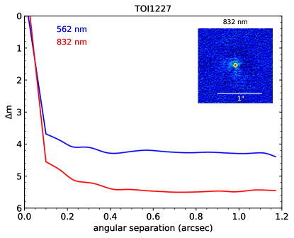
Figure 3: Detection limits from the Zorro speckle imager for TOI 1227. Detection limits from the two narrow-band filters (5620 Å and 8320 Å) are shown in blue and red, respectively. The sub-panel in the top right shows the narrow-band 8320Å, reconstructed image.

2.7 Limits on Wide Companions from Gaia EDR3 imaging

To identify potential wide binary companions that might exert secular dynamical influences on the TOI 1227 planetary system, we searched the Gaia EDR3 catalog (Gaia Collaboration et al., 2021) for comoving and codistant neighbors. While several candidate neighbors are found at projected separations of $\rho>500\arcsec$ (Section 3.1), none are found at $\rho<400\arcsec$ ($\rho\lesssim 40,000$ AU), the typical outer bound for observed binary companions for Sun-like stars (Raghavan et al., 2010) and well beyond the typical separation of mid-M binaries (Winters et al., 2019).

The nominal brightness limit of Gaia is $G_{lim}<21$ mag, which at an age of $\simeq$10 Myr approximately corresponds to a limit of $M_{lim}\simeq 14M_{Jup}$. Ziegler et al. (2018) and Brandeker & Cataldi (2019) have shown that Gaia is sensitive to companions with $\Delta G=6$ mag at $\rho>2\arcsec$ and $\Delta G=4$ mag at $\rho>1\arcsec$. Thus, Gaia would have identified almost all companions down to the separation regime where it meets the contrast limit of the Zorro speckle imaging (Section 2.6).

2.8 Archival Spectra from ESO

With the goal of better characterizing TOI 1227’s age, we retrieved the publicly available reduced spectra from the European Southern Observatory (ESO) archive for stars in the same population as TOI 1227 (Section 3). We downloaded any spectra of candidate members that included the Li line. In total, 11 objects had spectra from HARPS at the 3.6m telescope (La Silla Observatory), FEROS at the 2.2 m telescope (La Silla Observatory), and/or X-shooter at VLT (Cerro Paranal Observatory).

2.9 Archival Photometry, Astrometry, and Velocities

For TOI 1227 and all candidate members of the parent population (Section 3.1) we retrieved parallaxes, positions, proper motions, and photometry from Gaia Early Data Release 3 (EDR3; Gaia Collaboration et al., 2021; Lindegren et al., 2021; Riello et al., 2021). From EDR3 we also retrieved the Renormalised Unit Weight Error (RUWE) for all stars. RUWE value is effectively an astrometric reduced $\chi^{2}$ value, normalized to correct for color and brightness dependent effects. RUWE should be around 1 for well-behaved sources, and higher values (RUWE$\gtrsim$1.3) suggests with the presence of a stellar companion (Ziegler et al., 2020; Wood et al., 2021).

We downloaded velocities for candidate population members from a general Vizier/SIMBAD search, taking the most precise value for stars with multiple measurements. This yielded velocities for 21 stars. The full list of sources for these velocities is included in Table 5.

To aid with stellar characterization of TOI 1227, we also pulled photometry from the Two-Micron All-Sky Survey (2MASS; Skrutskie et al., 2006), the Wide-field Infrared Survey Explorer (WISE; Cutri & et al., 2014), and SkyMapper second Data Release (SkyMapper DR2; Onken et al., 2019).

3 The age and membership of TOI1227

Our Goodman spectrum of TOI 1227 showed strong H$\alpha$ emission and lithium absorption. Combined with TOI 1227’s high position on the color-magnitude diagram (CMD), this set an upper age limit of $<30$ Myr. However, we were able to derive a more precise estimate of the age of TOI 1227 from its parent population. To this end, we first identified likely members of the same association, then estimated the group age using rotation, lithium abundance, and fitting isochrones to the color-magnitude diagram.

3.1 The parent association of TOI 1227

To identify any co-moving and coeval population to TOI 1227, we first used the BANYAN-$\Sigma$ tool (Gagné et al., 2018), providing as input the IGRINS systemic velocity and the Gaia EDR3 position, parallax, and proper motion. This yielded a membership probability of 99.3% for $\epsilon$ Cha, with 0.4% for LCC and 0.3% for the field. However, TOI 1227 is $\simeq$25 pc away from the core of $\epsilon$ Cha, while nearly all known members of $\epsilon$ Cha are packed in a sphere $\lesssim$5 pc across (Murphy et al., 2013, also see Figure 4). The BANYAN algorithm preferred placing $\epsilon$ Cha over LCC likely because of better agreement in $UVW$ despite poor $XYZ$ agreement. However, the current BANYAN model did not account for more recent findings of significant velocity substructure in LCC (Goldman et al., 2018; Kerr et al., 2021), which changes the $UVW$ model for LCC and hence the membership probabilities.

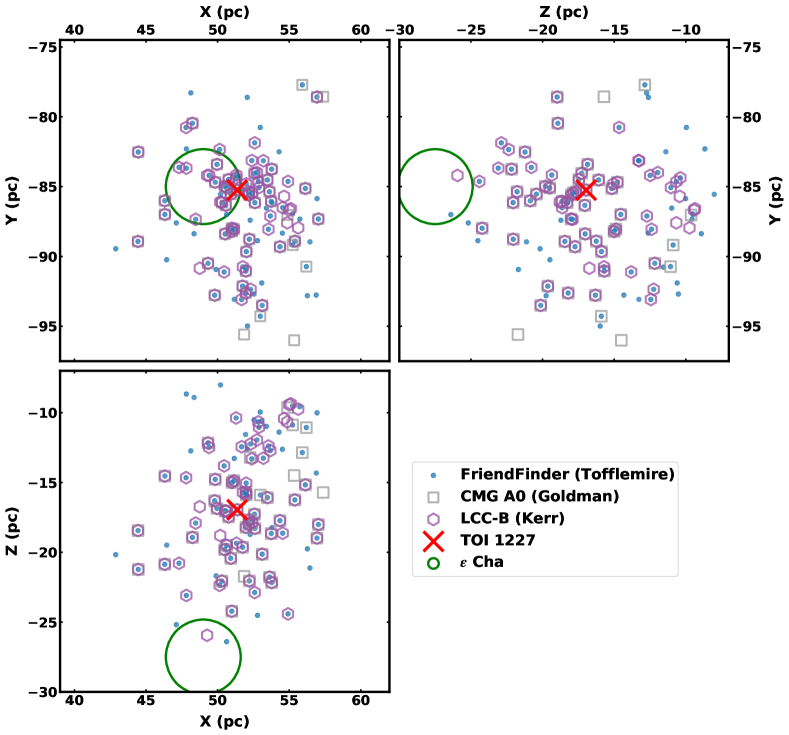
Figure 4: Galactic Heliocentric ($XYZ$) coordinates of 108 stars within the B subgroup of LCC (purple hexagons, Kerr et al., 2021), the A0 population of the Crux Moving Group (grey squares, Goldman et al., 2018), or stars identified using the FriendFinder algorithm restricted to $V_{\rm{tan},\rm{off}}<1$km s^-1 and within 10 pc of TOI 1227 (blue dots, Tofflemire et al., 2021). The planet host, TOI 1227, is marked with a red X, and is in all three lists. The significant overlap between these three selections re-affirms that these are all the same population, just selected using slightly different methods. For reference, we included a green circle that includes most of the known $\epsilon$ Cha members, highlighting that $\epsilon$ Cha is a separate and more compact population.

TOI 1227 was more recently identified as a member of the “B” sub-population of LCC by Kerr et al. (2021) and the A0 sub-group of the Crux Moving Group (CMG) by Goldman et al. (2018). These two groups are effectively the same, but use different selection methods and treatment of sub-groups. Kerr et al. (2021) considered this group (LCC-B) part of the LCC substructure, while Goldman et al. (2018) considered the CMG a moving group associated with LCC with multiple sub-groups (A0, A, B, and C). The $XYZ$ positions, proper motions, and available radial velocities of LCC-B/CMG-A0 members are similar to TOI 1227 (better so than $\epsilon$ Cha; Figure 4), so we adopted the LCC-B/CMG-A0 as the initial parent population.

We looked for additional members using the FriendFinder algorithm (Tofflemire et al., 2021). FriendFinder uses the Gaia EDR3 astrometry and radial velocity of a source (we used our IGRINS systemic velocity) to compute Galactic $UVW$ and $XYZ$, then projects the $UVW$ motion into the tangential velocities that would be expected for nearby stars if they were to share the same space motion. We selected stars with separations $<$10 pc from TOI 1227 and tangential velocities $<$1 km s^-1 from the expected values calculated by FriendFinder. These cuts were based on the fact that 1 km s^-1$\simeq$1 pc Myr^-1 and an estimated age for the population of $\simeq$10 Myr. We estimated these cuts would yield $\lesssim$2 field interlopers based on the background population of Gaia stars.

The three candidate membership lists–those from Goldman et al. (2018), Kerr et al. (2021), and this work–have significant overlap in both Galactic position and proper motion (Figures 4 and 5). Of the 108 stars in any of the three lists, 40 were in all three, and 27 were in two of the three. Further, most of the stars missing from Goldman et al. (2018) were missing precise parallaxes in Gaia DR2 (the former used DR2 while the other two selections used EDR3). Many of the stars in the FriendFinder list but not in Kerr et al. (2021) were removed by one of the quality cuts imposed by the latter work (e.g., $BP/RP$ flux excess). The FriendFinder list was also missing a small number of objects slightly further away from TOI 1227 because of our separation cut.

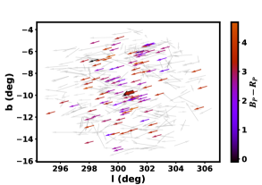
Figure 5: Galactic coordinates ($l$, $b$) of stars around TOI 1227, with arrows indicating the direction and magnitude of the proper motion for each star. Likely members of Musca (Section 3.1) are colored by their $B_{P}-R_{P}$ color. All star within 10 pc of TOI 1227 (excluding candidate members) are shown as grey arrows. TOI 1227 is thicker with a black outline.

To be inclusive, we adopted the combination of all three lists as the membership list for TOI 1227’s association; these 108 stars are listed in Table 5.

The resulting population has two (contradictory) names in the literature, both of which are difficult to remember. Given the presence of a young transiting planet, it deserves a more memorable name than ‘A0’ or ’B’. Most of the members land within the Musca constellation, so we refer to the merged group of stars as the Musca group (or just Musca).

TOI 1227 resides at the center of Musca, both based on Galactic position (Figure 4) and proper motion (Figure 5). The mean velocity of the members with literature RVs (12.8km s^-1) is also in good agreement with the value for TOI 1227. A randomly selected star that matches Musca in $XYZ$ has a $\ll$1% probability of matching Musca in proper motion and radial velocity by chance. The CMD also indicates a common age for stars in the population (Figure 6), with TOI 1227 matching the sequence. Combined with the presence of lithium in its spectrum, TOI 1227’s membership in Musca is unambiguous.

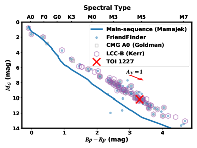
Figure 6: Color-magnitude diagram of stars in Musca (stars associated with TOI 1227), with symbols by the selection method or reference. We removed stars with poor astrometric fits from Gaia (RUWE$>1.5$; Gaia Collaboration et al., 2021). TOI 1227 is marked as an red ”X”, and lands within the tight sequence. The blue line indicates an empirical main-sequence for reference (Pecaut & Mamajek, 2013).

3.2 Rotation

To better measure the age of Musca (and hence TOI 1227), we measured rotation periods for all candidate members using TESS Full-Frame Images (FFIs) downloaded from the Mikulski Archive for Space Telescopes (MAST). First, we created initial light curves from the FFI cutouts centered on each candidate member. After background subtraction, we used the unpopular package (Hattori et al., 2021) to generate a Causal Pixel Model (CPM) of the telescope systematics for each star, which we subtracted from the initial light curve. We used the CPM curves because it does a better job preserving long-period signals than PDCSAP (Stello et al., 2016; Wang et al., 2017).

We searched the resulting single-sector light curves for rotation periods between 0.1–30 days using the Lomb-Scargle algorithm (Horne & Baliunas, 1986), repeating for each available sector. We selected the rotation period from the sector that returned the largest Lomb-Scargle power. As a check, we phase-folded the resulting light curves along that rotation period to inspect each measurement by eye. A few stars had multiple peaks in their Lomb-Scargle periodograms, which might indicate an unresolved binary. In such cases, we took the stronger signal (which was always the shorter period). Each rotation measurement was assigned a quality score during the visual inspection following Rampalli et al. (2021), with Q0 indicating an obvious rotation signal, Q1 a questionable signal, Q2 a spurious detection, and Q3 a light curve dominated by noise. In total, we measured usable rotation periods (Q0 or Q1) for 90 stars out of a sample of 108. Of the remaining 18, 11 were too faint to retrieve a reliable light curve, one showed a clear dipper pattern (and was identified as such by Tajiri et al., 2020), three had high flux contamination from nearby stars, and the remaining three had no significant period detection. Rotation period measurements are included in Table 5. The high detection rate is consistent with a young population and suggests a low rate of field-star interlopers in our selection.

The rotation period distribution (Figure 7) is consistent with the spread seen in the 10 Myr Upper Scorpius association (Rebull et al., 2018), and marginally consistent with the tighter rotation sequence at 40–60 Myr from Gagné et al. (2020). TOI 1227’s rotation period (1.65 days) was consistent with the Musca sequence. This effectively sets a limit of $\lesssim 60$ Myr for the group and further confirms TOI 1227 as a member.

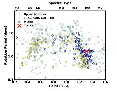
Figure 7: Rotation periods for candidate members of Musca (dark circles). Only stars with high-quality rotation periods (Q0 or Q1) are shown. For reference, we show rotation periods from $\simeq$10 Myr Upper Scorpius from Rebull et al. (2018) and 40-60 Myr ($\mu$ Tau, Carina, Columba, and Tucana-Horologium) from Gagné et al. (2020).

3.3 Lithium

Lithium (Li) is a powerful indicator of age in young stars (Chabrier et al., 1996). M dwarfs deplete their lithium over 10–200 Myr at a rate that depends on their spectral type; this forms a region where stars have no surface lithium (i.e., the lithium depletion boundary or LDB). The location and size of the LDB are strongly sensitive to the association’s age, and LDB ages are largely independent of the isochronal age (Soderblom et al., 2014). At the youngest ages ($<$20 Myr), lithium is only partially depleted, leading to a ‘dip’ in the Li levels short of a full boundary (Figure 8; also see Rizzuto et al., 2015). The location and depth of the lithium dip also depend strongly on age.

For our Li determinations, we measured the equivalent width of the Li 6708 Å line for 22 stars using our high-resolution ESO archival (11 targets) and Goodman (13 targets) spectra (two stars overlap). To account for the variations in resolution, $v\sin{i_{*}}$, and velocity between targets and the instrument used, we first fit nearby atomic lines with a Gaussian profile (e.g., iron lines for warmer stars and potassium lines for the M dwarfs). We used the width from these fits to define the bounds of the Li line. To estimate the pseudo-continuum, we iteratively fit the 6990–6720Å region excluding the Li line, each time removing regions $>$4$\sigma$ below the fit (there were no emission lines in this region). We did not attempt to correct for contamination from the Fe line at 6707.44 Å or broad molecular contamination in the cooler stars, which likely set a limit on the precision of our equivalent widths at the $\simeq$10% level.

A single star, TIC 359357695, had two clear sets of nearly equal-depth lines (an SB2). Interestingly, this star is a known TOI (1880), indicating a roughly equal-mass eclipsing binary. For the Li equivalent width, we measured each line individually with a manually-applied offset. We then combined the two equivalent widths.

In Figure 8b we compare the Li sequence for Musca to that from $\beta$ Pic ($\simeq$24 Myr; Shkolnik et al., 2017) and $\epsilon$ Cha (3-5 Myr; Murphy et al., 2013). The $\epsilon$ Cha cluster has high Li levels over the full sequence, while $\beta$ Pic showed a full depletion around M3–M5. Musca resides between these two, with a dip in Li levels around M3 but not full depletion; this effectively bounds the age of Musca between the two groups. Based on Li predictions from the Dartmouth Stellar Evolution Program (DSEP; Dotter et al., 2008) with magnetic enhancement (Feiden & Chaboyer, 2012), we estimated the Li age to be 8–14 Myr (Figure 8).

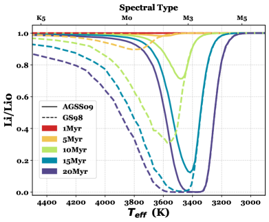
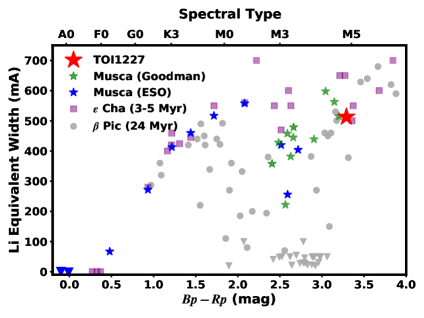
Figure 8: Left: Li abundance relative to the initial level predicted by the DSEP magnetic models for two different Solar abundance scales (dashed and solid lines) with colors corresponding to different times. The existence of a significant drop in the Li levels without a full depletion limits an association’s age to 8–14 Myr, depending on the assumed abundance scale (Grevesse & Sauval, 1998; Asplund et al., 2009). Right: lithium equivalent width of TOI 1227 (red) and its kinematic neighbors measured from Goodman (green star) or high-resolution ESO archival spectra (blue star). We compare this to the sequence from $\epsilon$ Cha (purple; Murphy et al., 2013), and $\beta$ Pic (grey; Shkolnik et al., 2017). Arrows indicate upper limits. $\epsilon$ Cha shows a clear sequence, while $\beta$ Pic shows full Li depletion around M2-M4. The stars associated with TOI 1227 show a dip around M3, but not a full depletion, bracketing the age between the two groups (5 Myr and 24 Myr). The top axis of both plots shows estimated spectral types.

3.4 Comparison to theoretical isochrones

We compared the candidate members of Musca to the PARSECv1.2S stellar isochrones (Bressan et al., 2012). To handle contamination from binaries and nonmember interlopers, we used a mixture model described in detail in Appendix A. We also removed stars with RUWE$>1.3$ (likely binaries) and stars outside the colors covered by the isochrones (i.e., stars with $M_{G}>11.8$ and $G-R_{P}>1.45$). Many tight pairs were resolved in Gaia, but not in 2MASS or similar ground-based surveys. The mixture model is not set up to handle these cases; a data point has a single outlier probability independent of the band. Thus, we performed this comparison using Gaia magnitudes only. An inspection of the sequence using 2MASS magnitudes suggested that this would not change the derived age in any significant way.

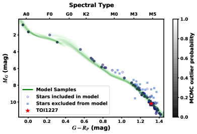
Figure 9: PARSEC isochrone fit to Musca members using a mixture model. The model comparison is done in color, but approximate spectral classes are given on the top axis. Stars included in the fit (blue circles) are filled based on their outlier probability. Excluded points (mostly due to a high RUWE) are shown as blue squares. The green lines are 200 random samples from the MCMC posterior. Models predict slightly different ages at different mass ranges; the mixture model takes the majority age by down-weighting stars in poorly matched regions (increasing their outlier probability).

The fit, shown in Figure 9, yielded an age of 11.6$\pm$0.5 Myr, consistent with 11.8 Myr from Goldman et al. (2018), 13.0$\pm$1.4 Myr from Kerr et al. (2021), and $\simeq$12 Myr for the lower end of LCC from Pecaut & Mamajek (2016). The age errors were likely underestimated, as our fit did not fully account for model systematics (often $\simeq$1-3 Myr, e.g., Bell et al., 2015). Indeed, the fit slightly underpredicted the luminosity of K2–K5 dwarfs and overpredicted the value for M4 and later. As an additional test, we repeated the fit using magnetic DSEP, which yielded a consistent age of 11.1$\pm$1.4 Myr, suggesting model differences are comparable to our measurement errors.

3.5 The age of Musca

Given the constraints from the isochrones, lithium, rotation, and the literature, we adopt an age of 11 Myr with a conservative uncertainty of $\pm$2 Myr. We used this age for TOI 1227 b as well, as any age spreads are likely to be similar to, or smaller than, the adopted uncertainties.

4 Host Star Analysis

We summarize properties of TOI 1227 in Table 3, the details of which we provide below.

Table 3: Properties of the host star TOI 1227.

Parameter	Value	Source
Identifiers
Gaia EDR3	5842480953772012928
TIC	360156606
2MASS	12270432-7227064
WISE	J122704.22-722706.5
Skymapper	397425267
Astrometry
$\alpha$ (J2016.0)	186.767344	Gaia EDR3
$\delta$ (J2016.0)	-72.451852	Gaia EDR3
$\mu_{\alpha}\cos{\delta}$ (mas yr-1)	-40.294$\pm$0.026	Gaia EDR3
$\mu_{\delta}$ (mas yr-1)	-10.808$\pm$0.030	Gaia EDR3
$\pi$ (mas)	9.9046$\pm$0.0242	Gaia EDR3
Photometry
GGaia (mag)	15.218$\pm$0.003	Gaia EDR3
BPGaia (mag)	17.195$\pm$0.006	Gaia EDR3
RPGaia (mag)	13.905$\pm$0.004	Gaia EDR3
V (mag)	17.00$\pm$1.13	TICv8.0
r’	16.346$\pm$0.013	Skymapper DR2
i’	14.333$\pm$0.009	Skymapper DR2
zs	13.523$\pm$0.007	Skymapper DR2
J (mag)	$11.890\pm 0.024$	2MASS
H (mag)	$11.312\pm 0.022$	2MASS
Ks (mag)	$11.034\pm 0.021$	2MASS
W1 (mag)	$10.887\pm 0.023$	ALLWISE
W2 (mag)	$10.649\pm 0.021$	ALLWISE
W3 (mag)	$10.516\pm 0.062$	ALLWISE
Kinematics & Position
RVBary (km  s-1)	13.3$\pm$0.3	This work
U (km  s-1)	-9.85$\pm$0.16	This work
V (km  s-1)	-19.88$\pm$0.25	This work
W (km  s-1)	-9.13$\pm$0.06	This work
X (pc)	51.34$\pm$0.16	This work
Y (pc)	-85.22$\pm$0.27	This work
Z (pc)	-16.95$\pm$0.05	This work
Physical Properties
$P_{\rm{rot}}$ (days)	$1.65\pm 0.04$	This work
$v\sin{i_{*}}$(km  s-1)	$16.65\pm 0.24$	This work
$i_{\star}$ (∘)	$>73$	This work
$F_{\mathrm{bol}}$ (erg cm-2 s-1)	($7.87\pm 0.53)\times 10^{-11}$	This work
Teff (K)	$3072\pm 74$	This work
SpT	M4.5V–M5V	This work
M⋆ (M⊙)	$0.170\pm 0.015$	This work
R⋆ (R⊙)	$0.56\pm 0.03$	This work
L⋆ (L⊙)	$(2.51\pm 0.17)\times 10^{-3}$	This work
$A_{V}$	$0.21^{+0.11}_{-0.09}$	This work
$\rho_{\star}$ ($\rho_{\odot}$)	$0.94\pm 0.18$	This work
Age (Myr)	11 $\pm$ 2	This work
LX (erg s-1)	1028.32	This work
log($L_{X}/L_{\rm{bol}}$) (dex)	-2.66	This work

4.1 Effective temperature, luminosity, radius, and mass

We first fit the spectral-energy-distribution (SED) following the methodology from Mann et al. (2016a) and highlighted in Figure 10. To briefly summarize, we compared the observed photometry and Goodman spectrum to a grid of template spectra drawn from nearby (likely reddening-free) young moving groups. The observed data was simultaneously fit with Solar-metallicity BT-SETTL CIFIST models (Baraffe et al., 2015). The atmospheric models were used both to estimate $T_{\text{eff}}$ and fill in gaps in the template spectra (e.g., beyond 2.3 $\mu$m). We combined this full SED with the Gaia EDR3 parallax to estimate both the bolometric flux ($F_{\mathrm{bol}}$) and the total luminosity ($L_{*}$). With $T_{\text{eff}}$ and $L_{*}$, we calculated the stellar radius ($R_{*}$) using the Stefan-Boltzmann relation. The fit included six total free parameters: the choice of template, $A_{V}$, $T_{\text{eff}}$, and three parameters that account for flux and wavelength calibration offsets between the Goodman spectra, stellar templates, and model spectra. To account for variability in the star, we added (in quadrature) 0.03 mags to the errors of all optical photometry. The resulting fit yielded $T_{\text{eff}}$$=3072\pm 84$ K, $F_{\mathrm{bol}}$$=(7.87\pm 0.53)\times 10^{-11}$ erg cm^-2 s^-1, $L_{*}=(2.51\pm 0.17)\times 10^{-3}\,L_{\odot}$, $A_{V}=0.21^{+0.11}_{-0.09}$ mag, and $R_{*}=0.56\pm 0.03\,R_{\odot}$. Swapping to the PHOENIX model grid from Husser et al. (2013) yielded nearly identical $F_{\mathrm{bol}}$ and a higher (but consistent) $T_{\text{eff}}$ of 3145$\pm$67 K.

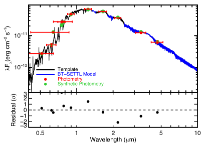
Figure 10: Example fit from comparing BT-SETTL models and young un-reddened templates to the observed photometry and Goodman spectrum. The red points are the observed photometry converted to fluxes using the appropriate zero-point and uncertainty, with the vertical errors denoting the uncertainties and the horizontal errors the approximate filter width. Green points are synthetic photometry derived from combining the spectrum with the relevant filter profile. The bottom panel shows the residual in standard deviations. TOI 1227 was not detected in WISE $W4$ and the $W3$ point is not shown for clarity (but is used in the fit). The template/model shown here (black) is an M4.5-M5 star in the $\beta$ Pic association and a 3075 K model (blue).

During the fit, the surface-brightness predictions of the atmospheric models were scaled to match the observed photometry. The scale factor is equivalent to $R_{*}^{2}/D^{2}$, which combined with the Gaia EDR3 parallax, provided an additional estimate of $R_{*}$. The technique is similar to the infrared flux method (IRFM; Blackwell & Shallis, 1977). IRFM-based radii of low-mass stars have not consistently agreed with empirical measurements (Casagrande et al., 2008; Boyajian et al., 2012), but more recent efforts have been more successful (Morrell & Naylor, 2019), and our resulting $R_{*}$ estimate ($0.57\pm 0.03\,R_{\odot}$) was consistent with our estimate using the Stefan-Boltzmann relation.

We also derive $T_{\text{eff}}$ using our IGRINS spectra. While we consider the SED-based estimate to be reliable, we were concerned about significant spot coverage impacting our derived $T_{\text{eff}}$ (and hence $R_{*}$). Spot coverage would manifest as a cooler temperature at redder wavelengths, where the (cooler) spots have a larger impact on the total flux. Hot spots would have the opposite effect, which would also be visible as a wavelength-dependent $T_{\text{eff}}$. The IGRINS data offers another advantage here; $T_{\text{eff}}$ determined from the low-resolution Goodman spectra was driven by the molecular bands, while the high-resolution $H$- and $K$-band data from IGRINS are less sensitive to missing or erroneous molecular opacities. Thus, while the two fits use the same BT-SETTL models, the fits using IGRINS data were sensitive to different systematics in those models (Rajpurohit et al., 2018).

We fit the highest SNR IGRINS spectra obtained. We fit each order separately, but only included orders with low telluric contamination (determined by eye) and SNR $>$80. For each fit, we explored six free parameters: $T_{\text{eff}}$, $\log~{}g$, radial velocity, a broadening parameter (including instrumental and rotational effects), the coefficients of the first two Chebyshev polynomials (used to correct for flux calibration offsets), and a factor that describes missing uncertainties in the data as a fraction of the observed spectrum. We fixed [Fe/H] to Solar, consistent with measurements of young regions around Sco-Cen (James et al., 2006). We fit all free parameters using the Monte Carlo Markov Chain code emcee (Foreman-Mackey et al., 2013). Each order was run with 30 walkers for 50,000 steps after an initial burn-in of 10,000 steps and with uniform priors bounded only by the model grid or physical limits.

Parameters besides $T_{\text{eff}}$ were effectively nuisance parameters in this analysis, as most other parameters (e.g., $v\sin{i_{*}}$) were better determined with more empirical methods. We summarize the $T_{\text{eff}}$ results in Figure 11. $T_{\text{eff}}$ measurements from a given order were often precise (typical errors of 15–50 K), but varied between orders by 50–100 K; we considered the latter a more accurate reflection of the true errors, as systematics in the models change with wavelength. The $T_{\text{eff}}$ for each order was generally consistent with our fit to the SED and optical spectrum, indicating that our derived $T_{\text{eff}}$ was reliable and spots (while still present) did not significantly impact our derived $T_{\text{eff}}$.

We repeated our fit to the IGRINS data after co-adding all 11 spectra. Because the spectra were taken across the rotational phase, these likely sample different spot coverage patterns. However, the resulting spectrum was significantly higher SNR ($>200$). The results were broadly consistent, with smaller errors in each order (10–30 K) but a similar variation between orders (50–100 K). The variation between orders was not consistent with the effect of spots, further suggesting that the spread in inferred $T_{\text{eff}}$ was driven by systematics in the models, rather than observational noise or surface inhomogeneities on the host.

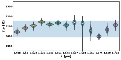
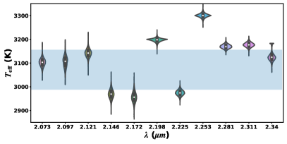
Figure 11: Marginal probability distributions on $T_{\text{eff}}$ (’violin’ plot; Waskom et al., 2020) for 24 IGRINS orders fit independently over the $H$- (left) and $K$-band (right). Each violin has an equal area distributed according to the MCMC posterior, so narrow/tall violins represent larger uncertainties than wider/shorter ones. The blue bar represents the 1$\sigma$ distribution from our optical spectrum and SED fit.

To determine $M_{*}$ and as an additional check on our stellar parameters above, we compared the observed photometry to Solar-metallicity magnetic DSEP evolution models. We compared Gaia and 2MASS absolute magnitudes to the model predictions with an MCMC framework using emcee. We fit for age, $A_{V}$, and $M_{*}$. An additional parameter ($f$, in magnitudes) captured underestimated uncertainties in the data or models. We used a hybrid interpolation method that found the nearest age in the model grid and then performed linear one-dimensional interpolation in mass to obtain stellar parameters and synthetic model photometry. To account for errors from our nearest-age approach and ensure uniform sampling in age, we pre-interpolated bilinearly in age and mass using the isochrones package (Morton, 2015). The interpolated grid was far denser (0.1 Myr and 0.01$M_{\odot}$) than expected errors. To redden the model photometry, we used synphot (Lim, 2020), following the extinction law from Cardelli et al. (1989). We placed Gaussian priors for age (11$\pm$2 Myr; derived from the population), $A_{V}$ (0.21$\pm$0.1 mag; from the SED fit), and $T_{\text{eff}}$ (3072$\pm$74 K; from the SED fit). All other parameters evolved under uniform priors. From the best-fit posteriors, we were able to interpolate additional posteriors on other stellar parameters from the evolutionary model, including $R_{*}$ and $T_{\text{eff}}$.

The fit yielded $\text{age}=11.5\pm 1.0$ Myr, $M_{*}=0.165\pm 0.010\,M_{\odot}$, $A_{V}=0.148\pm 0.074$ mag, $R_{*}=0.554\pm 0.007\,R_{\odot}$, and $T_{\text{eff}}=3050\pm 20$ K. Changing the $T_{\text{eff}}$ prior to uniform yielded consistent, but less precise parameters (e.g., $M_{*}=0.170\pm 0.015M_{\odot}$). As an additional test, we repeated the analysis using the PARSEC models, which yielded parameters somewhat discrepant with our SED and population analysis ($\text{age}=14.9\pm 2.1$ Myr, $T_{\text{eff}}=2900\pm 30$ K, and $M_{*}=0.20\pm 0.01\,M_{\odot}$). PARSEC did not reproduce the observed colors of the coolest stars in Musca, which manifested as systematically high luminosities for a fixed color past $\simeq$M4 (see Figure 9). Thus, we prefer the magnetic DSEP fit. However, we adopted the more conservative mass ($M_{*}=0.170\pm 0.015\,M_{\odot}$), which was $2\sigma$ consistent with the PARSEC value.

4.2 Rotation period, rotational broadening, and stellar inclination

Canto Martins et al. (2020) reported a rotation period ($P_{\rm{rot}}$) of 1.663$\pm$0.028 days for TOI 1227 using TESS data. Our analysis of rotation periods in Section 3 yielded a consistent 1.65$\pm 0.04$ days, which we adopted for our analysis. We computed $v\sin{i_{*}}$ as part of extracting radial velocities from IGRINS/Gemini and HRS/SALT spectra. The mean value from the IGRINS data was 16.65$\pm$0.24 km s^-1, while the SALT data yielded a marginally inconsistent value of 17.8$\pm$0.3 km s^-1. We adopted the former value, as the IGRINS data are significantly higher SNR and less impacted by spots or molecular line contamination.

We used the combination of $v\sin{i_{*}}$, $P_{\rm{rot}}$, and $R_{*}$ to estimate the stellar inclination ($i_{*}$), and hence test whether the stellar spin and planetary orbit are consistent with alignment. A basic version of this calculation can be done by estimating the $V$ term in $v\sin{i_{*}}$ using $V=2\pi R_{*}/P_{\rm{rot}}$, although in practice it requires additional statistical corrections, including the fact that we can only measure alignment projected onto the sky. To this end, we followed the formalism from Masuda & Winn (2020). The resulting stellar inclination was consistent with alignment with the planet, yielding a limit on inclination of $i_{*}>73^{\circ}$ at 95% confidence, and $i_{*}>77^{\circ}$ at 68% confidence.

4.3 X-Ray Luminosity

TOI 1227 was detected in X-rays in a ROSAT pointing of the globular cluster NGC 4372 in 1993 (Johnston & Verbunt, 1996). The X-ray source was listed as #6 in the NGC 4372 (IDed in SIMBAD as [JVH96] NGC 4372 6), however, the quoted values were not usable here, as they quote an X-ray flux assuming that the source is at the distance to NGC 4372 and only gave upper limits on the hardness ratios. The X-ray detection was reanalyzed by Voges et al. (2000) in the 2nd ROSAT PSPC Catalog, which IDs the X-ray source as 2RXP J122703.8-722702, situated 4.9″ away from TOI 1227 with a positional error of $\pm$9″  (i.e. consistent with TOI 1227 being the source of the X-rays). They list a soft X-ray count rate of $f_{X}$ = (1.967 $\pm$ 0.626) $\times$ 10^-3 ct s^-1 with hardness ratios HR1 = 0.06 $\pm$ 0.32 and HR2 = 0.58 $\pm$ 0.32 with an effective exposure time of 7399 s observed over UT 4-6 September 1993. Using the energy conversion factor equation of Fleming et al. (1995), this count rate and HR1 hardness ratio translates to a soft X-ray energy flux of $f_{X}$ = 1.70 $\pm$ 10^-14 erg s^-1 cm^-2, which at the distance to TOI 1227  translates to a soft X-ray luminosity of L_X = 10^28.32 erg s^-1.

Given our estimate of the star’s bolometric luminosity (Table 3), this translates to a fractional X-ray luminosity of log(L_X/L_bol) = $-$2.66. This is within the range of activity levels stars in the saturated regime display. However, X-ray levels tell us little about TOI 1227’s age; M5V stars remain in the saturated well into field ages (West et al., 2015; Newton et al., 2017).

5 Transit Analysis

We fit the TESS, SOAR, and LCO photometry simultaneously using the MISTTBORN (MCMC Interface for Synthesis of Transits, Tomography, Binaries, and Others of a Relevant Nature) fitting code first described in Mann et al. (2016b) and expanded upon in Johnson et al. (2018). MISTTBORN uses BATMAN (Kreidberg, 2015) to generate model light curves and emcee (Foreman-Mackey et al., 2013) to explore the transit parameter space using an affine-invariant Markov chain Monte Carlo (MCMC) algorithm.

We used MISTTBORN to fit for the five regular transit parameters: time of inferior conjunction ($T_{0}$), orbital period of the planet ($P$), planet-to-star radius ratio ($R_{p}/R_{\star}$), impact parameter ($b$), and stellar density ($\rho_{\star}$). For each wavelength observed, we included two linear and quadratic limb-darkening coefficients ($q_{1}$, $q_{2}$) following the triangular sampling prescription of Kipping (2013). We included data from four unique bands: TESS, $g$’, $i$’, and $z_{s}$, requiring eight limb-darkening parameters in total ($r$’ was not used for reasons detailed below). Gas drag and gravitational interactions are expected to dampen out eccentricities and inclinations of extremely young planets like TOI 1227 b (Tanaka & Ward, 2004), so we locked the eccentricity to zero (although we check this assumption later).

To model stellar variations, MISTTBORN included a Gaussian Process (GP) regression module, utilizing the celerite code (Foreman-Mackey et al., 2017). We initially followed the procedure in Foreman-Mackey et al. (2017), using a mixture of two stochastically driven damped simple harmonic oscillators (SHOs) at periods $P_{GP}$ (primary) and $0.5P_{GP}$ (secondary). However, we found the second signal was poorly constrained, suggesting a single SHO was sufficient. Instead, we adopted a fit that included three GP terms: the dominant period ($\ln{P_{GP}}$), amplitude ($\ln{\rm{Amp}}$), and the decay timescale for the variability (quality factor, $\ln{Q}$).

Stellar variation from spots is wavelength-dependent. This raised a problem when fitting multiple transits over such a wide wavelength range with a single GP amplitude. The most robust solution would be to fit the data using multiple GPs with a common period (e.g., GPFlow; Matthews et al., 2017). However, most of the ground-based transits were partials and many lacked significant out-of-transit baseline, so the GP is poorly constrained from an individual transit. Further, our GP kernel was able to fit nonsimultaneous data of multiple wavelengths, because the rotation signal can evolve during the 27 days between transits. In cases where we had simultaneous data from multiple filters (3 transits), we used only the more precise dataset. This cut excluded all $r$’ data but still left us with nine observed transits (6 from the ground). We used the excluded observations for our false-positive analysis (specifically the test of chromaticity; Section 6).

When handling crowded regions and faint sources like TOI 1227 (see Figure 1), the SPOC reduction of TESS data has been known to over subtract the sky background (Burt et al., 2020), leading to a deeper transit depth. This was a potential issue for data collected before Sector 27, after which SPOC applied a correction to their reduction. An initial fit of our data yielded TESS depths somewhat deeper than the ground-based transits, and the Sector 11-12 data deeper than the Sector 38 data. To correct for this, we re-analyzed the target pixel files and estimate that the PCDSAP light curves required an additive correction of 37e^-1 pixel^-1 for Sector 11 and 75e^-1 pixel^-1 for Section 12. No significant bias was seen for the Sector 38 data. We applied this correction to the light curve before running MISTTBORN, and to account for uncertainties we fit for two dilution terms ($C_{S11}$ and $C_{S12}$) applied to the TESS Sector 11 and 12 data following Newton et al. (2019):

$$LC_{\rm{diluted}}=\frac{LC_{\rm{undiluted}}+C}{1+C},$$ (1)

where $LC_{\rm{undiluted}}$ was the model light curve generated by MISTTBORN. A negative dilution would correspond to ovsersubtraction of the background (i.e., if the corrections above were underestimated).

We applied Gaussian priors on the limb-darkening coefficients based on the values from the LDTK toolkit (Parviainen & Aigrain, 2015), with errors accounting for errors in stellar parameters and the difference between models used (which differ by 0.04-0.08). All other parameters were sampled uniformly with physically motivated boundaries (e.g., $|b|<1+R_{P}/R_{*}$, $0<R_{P}/R_{*}<1$, and $\rho_{*}>0$).

We ran the MCMC using 50 walkers for 500,000 steps including a burn-in of 50,000 steps. This run was more than 50 times the autocorrelation time for all parameters, indicating it was more than sufficient for convergence.

All output parameters from the MISTTBORN analysis are listed in Table 4, with a subset of the parameter correlations in Figure 12. Combining the derived $R_{P}/R_{\star}$ with our estimated stellar parameters from Section 4 yielded a planet radius of $R_{P}=0.854^{+0.067}_{-0.052}R_{J}$.

Table 4: Global Transit-Fit Parameters.

Parameter	with GP	No GP
Transit Fit Parameters
$T_{0}$ (BJD-2457000)	$1617.4621\pm 0.0016$	$1617.4627\pm 0.001$
$P$ (days)	$27.36397\pm 0.00011$	$27.363916\pm 7.9\times 10^{-5}$
$R_{P}/R_{\star}$	$0.1568^{+0.009}_{-0.0047}$	$0.1546^{+0.0035}_{-0.0024}$
$b$	$0.849^{+0.024}_{-0.015}$	$0.836^{+0.014}_{-0.012}$
$\rho_{\star}$ ($\rho_{\odot}$)	$0.755^{+0.062}_{-0.072}$	$0.735\pm 0.049$
$q_{1,TESS}$	$0.32\pm 0.12$	$0.21\pm 0.10$
$q_{2,TESS}$	$0.293^{+0.082}_{-0.083}$	$0.275\pm 0.083$
$q_{1,g}$	$0.74\pm 0.12$	$0.80\pm 0.10$
$q_{2,g}$	$0.384^{+0.057}_{-0.059}$	$0397\pm 0.056$
$q_{1,i}$	$0.56\pm 0.11$	$0.619\pm 0.090$
$q_{2,i}$	$0.336^{+0.071}_{-0.073}$	$0.358\pm 0.068$
$q_{1,z}$	$0.27\pm 0.12$	$0.299^{+0.093}_{-0.088}$
$q_{2,z}$	$0.283^{+0.08}_{-0.081}$	$0.287\pm 0.080$
$C_{S11}$	$-0.081^{+0.11}_{-0.092}$	$-0.06\pm 0.08$
$C_{S12}$	$0.04^{+0.12}_{-0.1}$	$0.03\pm 0.09$
$\ln(P_{GP})$	$0.532^{+0.051}_{-0.037}$	…
$\ln(Amp)$	$-10.39^{+0.15}_{-0.14}$	…
$\ln(Q)$	$1.14^{+0.23}_{-0.20}$	…
Derived Parameters
$a/R_{\star}$	$34.01^{+0.97}_{-1.0}$	$34.48^{+0.75}_{-0.79}$
$i$ (∘)	$88.571^{+0.062}_{-0.093}$	$88.611^{+0.047}_{-0.054}$
$T_{14}$ (days)	$0.2013^{+0.0049}_{-0.0043}$	$0.2013^{+0.0029}_{-0.0027}$
$R_{P}$ ($R_{J}$)	$0.854^{+0.067}_{-0.052}$	$0.842^{+0.049}_{-0.047}$
$a$ (AU)	$0.0886^{+0.0054}_{-0.0057}$	$0.0898\pm 0.0052$
$S$ ($S_{\oplus})$	$3.21^{+0.38}_{-0.36}$	$3.12\pm 0.33$

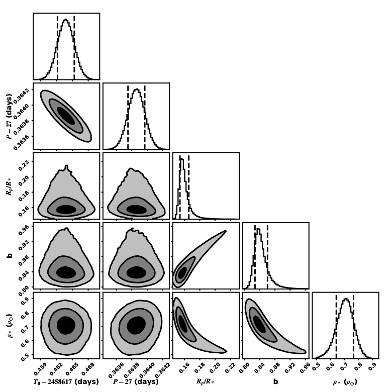
Figure 12: Corner plot of the major transit parameters (GP and limb-darkening parameters excluded for clarity). Most parameters are roughly Gaussian although $R_{P}/R_{*}$ and $b$ have a long tail corresponding to a high impact parameter and larger planet. At the extreme ($R_{P}/R_{*}=0.22$), this would still correspond to a planetary radius (1.2$R_{J}$).

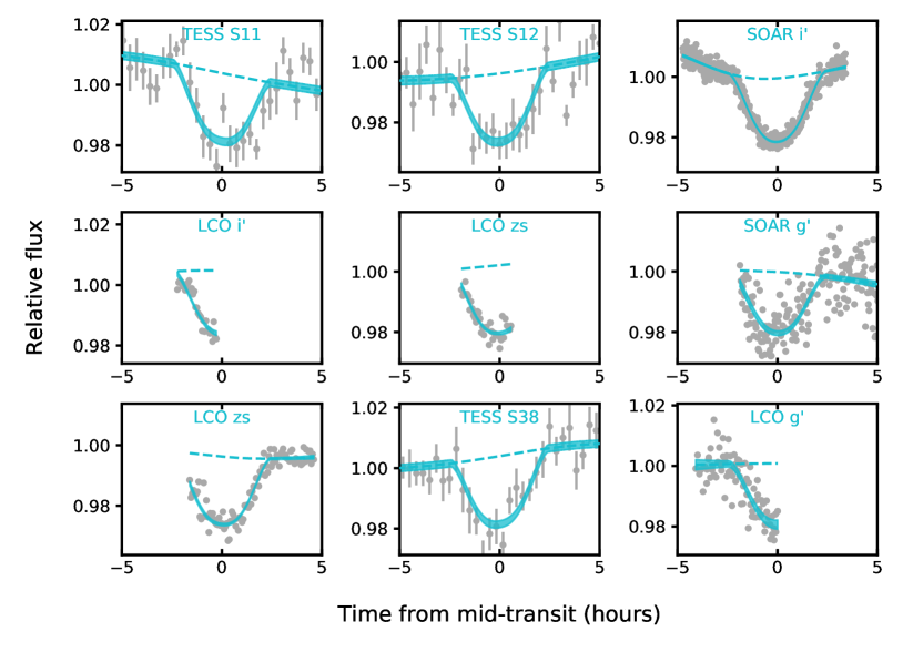
Figure 13: All nine transits from TESS (3 transits) and ground-based follow-up (6 transits) that were used in our MCMC global fit, shown in chronological order. The cyan shaded region shows the combined GP and transit model. The dashed line shows the GP fit absent the transit model. The scales of all panels match. For clarity, we have binned the TESS data and show the scatter in each bin as error bars; for all other light curves, one point represents one exposure.

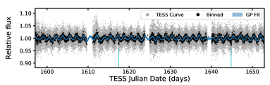
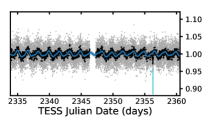
Figure 14: TESS light curve from Sectors 11 and 12 (left) and 38 (right). PDCSAP light curve in grey with binned points in black. The GP model fit is shown as a blue shaded region (indicating 1$\sigma$ range); outside of gaps in coverage, errors on the GP fit are usually too small to see. The three cyan vertical lines mark the location of TOI 1227 b transits.

The resulting fit from MISTTBORN reproduced the individual transits (Figure 13) as well as the overall light curve variations seen in TESS (Figure 14). The dilution parameters were both consistent with zero, suggesting our corrections to the PDCSAP curves were reasonable. The transit depth and stellar radius gave a planet radius of $0.859^{+0.065}_{-0.052}\,R_{J}$ ($9.6\pm 0.7\,R_{\oplus}$). The posterior showed a tail at larger radii, corresponding to a higher impact parameter (Figure 12). At $99.7$% confidence TOI 1227 b is $<$1.2 $R_{J}$ ($13.4\,R_{\oplus}$).

Including the GP was computationally expensive, which led us to use the (binned) 120 s TESS data from Sector 38 (although 20 s data was available). As discussed above, a single GP fitting chromatic variability over multiple wavelengths and a long time period may be misleading. As a test, we refit the transit without the GP, removing the stellar variability before running the MCMC fit. For the TESS data, we fit the shape of the transits and the low-frequency variability simultaneously following Pepper et al. (2020), then divided out the variability model. For the ground-based transits, we fit each transit individually including the GP model as above (such that each transit can have a unique GP amplitude) and divided out the best-fit GP model from the light curve. Because most of the ground-based photometry had a limited out-of-transit baseline, only four of the transits were used.

We ran the GP-free fit through MISTTBORN for 200,000 steps after a burn-in of 20,000 steps. Priors were the same as from our earlier fit.

The GP-free fit was largely consistent with our GP fit, but with smaller uncertainties. The resulting fit parameters are listed in Table 4. We also show the phase-folded transit data in Figure 15.

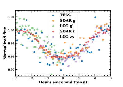
Figure 15: Phase-folded transit data from TESS and four ground-based transits after removing stellar variability. The TESS and SOAR $i^{\prime}$ data have been binned for clarity. Dilution on TESS data has been removed. The transit shape varies slightly due to differences in limb darkening, but the transit parameters generally agree.

We assumed zero eccentricity for both fits, but any nonzero eccentricity might (depending on the argument of periastron) manifest difference between our stellar density derived in Section 4 and the value from the fit to the transit. The transit-fit density agreed with the spectroscopic value. However, the spectroscopic and isochronal parameters are far less precise and eccentricities inferred this way are degenerate with the argument of periastron. Thus, we can only say that a low eccentricity ($<0.2$) is preferred.

The transit-fit density is more than a factor of two more precise than the value estimated from our SED fit and stellar models (Section 4). If the $e=0$ assumption is valid, the transit-fit density could be used to improve the estimated $R_{*}$ (e.g., Seager & Mallén-Ornelas, 2003; Sozzetti et al., 2007). However, this provided only a marginal improvement on the $R_{*}$ uncertainty (0.0250$R_{\odot}$ vs 0.030$R_{\odot}$) due to a large error on $M_{*}$. Since the $M_{*}$ estimate is model-dependent, we opted to keep the stellar parameters from Section 4.

6 False-positive Analysis

We considered the three most common false positive (non-planetary) scenarios to explain the transit signal: an eclipsing binary, a background eclipsing binary, and a hierarchical (bound) eclipsing binary. Other scenarios that may apply specifically to young stars (e.g., stellar variability) were quickly dismissed due to the depth, duration, and shape of the transit, as well its consistency over more than a year.

6.1 Eclipsing Binary

We compared the radial velocity (RV) data from IGRINS (Table 2) to the predicted velocity curve of a planet or binary at the orbital period of the outer planet (27.4 d). We did not use HRS data for this analysis. There may be zero-point offsets between velocities from IGRINS and HRS. HRS velocities also showed significantly higher velocity scatter ($>$500 m s^-1), likely due to higher stellar variability in the optical.

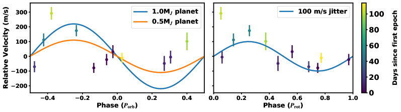
Figure 16: Radial velocities of TOI 1227 from IGRINS (Section 2.5.3) phased to the period of the planet (left) or the rotation period (right). Points are color-coded by time since the first epoch. For reference, we show the expected variations for 0.5$M_{J}$ ($\simeq 110$m s^-1, orange) and 1$M_{J}$ planets ($\simeq$220m s^-1, blue) in then left figure and a simple 100m s^-1 jitter (blue) from stellar rotation (right). The velocities are consistent with a $\simeq$100m s^-1 jitter from rotation. HRS velocities are less precise and there may be zero-point differences between the two instruments, so they are not shown here.

A Jovian-mass planet would induce an RV signal of $\simeq$220 m s^-1, while the scatter in the IGRINS velocities was $\simeq$130 m s^-1 (Figure 16), ruling out even a highly eccentric brown dwarf. There was a marginal detection of a $\sim$0.5 $M_{J}$ planet, particularly if we allow the planet’s orbit to be slightly eccentric. However, a modest stellar jitter expected from rotation and long-term variation in the spot pattern could explain all of this variation. Denser sampling and a full radial velocity model including stellar noise would be more likely to yield a detection, but we can still place an upper limit of $M_{P}<1.7\,M_{J}$ at $>$95% confidence. This rules out any possible brown dwarf companion.

6.2 Background Eclipsing Binary

Given a maximum eclipse depth of 50% and an observed transit depth of 2.5%, the star producing the observed signal must be within $\Delta m<3.26$ mags of TOI 1227. Since the depth is consistent across all filters, this constraint applies to all $griz$ magnitudes. The multi-band speckle data (Section 2.6) ruled out such a companion or background star down to 90 mas. Vanderburg et al. (2019) detail a similar metric based on the ratio of the ingress time ($T_{12}$) to the time between first and third contact ($T_{13}$). However, because TOI 1227 b has a high impact parameter, this metric gives marginally worse constraints than the transit depth alone.

The proper motion of TOI 1227 was large enough to see ‘behind’ the source using digitized images (DSS) from the Palomar Observatory Sky Survey (POSS-I, POSS-II) and the Southern ESO Schmidt (SERC) Survey (patient imaging; Muirhead et al., 2012; Rodriguez et al., 2018). Between the blue POSS images (1976.3) and the most recent SOAR transit data (2021.2), TOI 1227 moved more than 1.8″. This motion was much larger than the resolution of our SOAR transit imaging ($\simeq 0.8\arcsec$) and speckle imaging (0.09″), and somewhat larger than the resolution of the POSS plates (1.7″). No source was present in the DSS images at the modern location of TOI 1227. After subtracting the source using a nonparametric model of the PSF from StarFinder (Diolaiti et al., 2000), we were able to rule out any source $<$3 magnitudes fainter than TOI 1227. Additionally, both USNO-A2.0 and USNO-B reported no other nearby sources data (Monet et al., 2003), but were sensitive to stars $>$3 magnitudes fainter than TOI 1227 (in $R$).

6.3 Hierarchical Eclipsing Binary

To check for a bound companion eclipsing binary, we first ran the MOLUSC code (Wood et al., 2021). MOLUSC simulated binary companions following an empirically-motivated random distribution in binary parameters. We limited the mass of the synthetic companions to between 10 $M_{J}$ to 0.17 $M_{\odot}$, as the goal was only to identify any unseen stellar or brown dwarf companion. For each synthetic binary, MOLUSC computed the corresponding velocity curve, brightness, and (sky-projected) separation, as well as enhancement to the noise that would be measured by Gaia. The results were compared directly to our observed high-resolution images, radial velocities, and the Gaia astrometry. When running MOLUSC, we included all radial velocity data, high-resolution imaging, Gaia astrometry, and limits implied by TOI 1227’s CMD position compared to the population (the latter effectively rules out companions $<$0.3 mag fainter than TOI 1227 at Gaia bandpass and resolution). In total, MOLUSC generated 5 million synthetic companions and determined which could not be ruled out by the data (survivors).

MOLUSC found that only 9% of the generated companions survived (Figure 17). Most of the survivors were faint or stars on wider orbits that happen to have orbital parameters that put them behind or in front of TOI 1227 during all observations. Furthermore, when we restricted the survivors to those that could reproduce the observed transit (unresolved in imaging and sufficiently bright for the observed transit), only 1% of the possible companions remained.

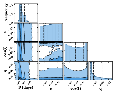
Figure 17: Distribution of surviving companions from MOLUSC in period ($P$), eccentricity ($e$), cosine of the inclination ($\cos(i)$) and mass ratio ($q$). The distribution represents only 9% of the total generated companions, the rest of which were ruled out by the observational data.

We also used the transit depths measured independently in each of the observed filters to measure the color of any potential undetected companions. At redder wavelengths, the contrast ratio of the primary and companion approaches unity, so a transit or eclipse from the redder companion would appear deeper in the longer-wavelength data. Désert et al. (2015) and Tofflemire et al. (2019) showed how to convert the ratio of the transit depths for any two bands ($\delta_{2}/\delta_{1}$) into the difference in colors between the target and any potential companion:

$$m_{1,c}-m_{2,c}<m_{1,p}-m_{2,p}+2.5\rm{log}\left(\frac{\delta_{2}}{\delta_{2}}\right),$$ (2)

where $m_{1,x}-m_{2,x}$ is the color of the primary ($p$) or companion ($c$).

We excluded TESS from this comparison because of the ambiguity introduced by the dilution term (Section 5). We also excluded the LCO $g^{\prime}$ data observed on 2021 Apr 24 (see Section 6.4 for more details). We split the data into four datasets corresponding to the four observed filters; we combined the ASTEP $R_{c}$ data with the SDSS $r$’ data for simplicity, although our coverage in this is poor and the result did not have a significant impact when compared to the effect of other observations taken at other wavelengths. We then fit the dataset for each filter independent of the others. Our fit followed the same method outlined in Section 5, but we placed priors on the wavelength-independent parameters ($\rho$, $b$, $P$, $T_{0}$, and $\ln(P_{GP})$) drawn from our global fit.

As we show in Figure 18, all transits yielded consistent depths. The deepest transits were the two bluest: $g^{\prime}$ and $r^{\prime}$ (although $r$’ depth was very uncertain). A bound eclipsing binary would have yielded a shallower transit at the bluest wavelengths. Taking the 95% confidence of the depth ratio, any companion harboring the transit/eclipse signal must be $<$0.06 mag redder than TOI 1227 in $g-z$. To satisfy these color criteria, the companion would have to be approximately equal mass to TOI 1227, making the two appear brighter by $>$0.3 mag in $G$. However, TOI 1227 sat within $0.2$ mag of the group CMD (Figure 9). More quantitatively, the resulting tight color constraints eliminated all surviving companions from the MOLUSC analysis, ruling out this scenario and validating the signal as planetary.

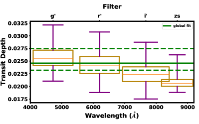
Figure 18: Box and whisker plot of the ground-based transit depths. The orange line indicates the median of each fit, with boxes indicating the 1$\sigma$ range and whiskers the 2$\sigma$ range. The global fit is shown as a green line with dashed lines corresponding to the 1$\sigma$ range. The width of each box roughly corresponds to the filter width. If the transit signal were due to an eclipse around a redder companion (or background star), the transit should be deeper in the red where the flux ratio is closer to unity. The opposite was seen; transits were deeper in $g$ than in $z_{s}$ (although all transit depths were consistent).

6.4 The unusual April 2021 transit

We excluded the $g^{\prime}$ LCO transit from 2021 Apr 24 in our above analysis. The observations missed ingress but covered most of the transit, all of the egress, and about 1.5 h post-transit. Before color corrections, no clear transit was detected, and even with variability and color corrections the transit was weaker than expected (Figure 19). While the scatter in the data was large (1.5%), the data suggested a maximum transit depth of $\simeq$1%. That same transit was observed simultaneously in $z_{s}$, which showed the expected shape; and in $R_{c}$, which showed an egress as expected. Although the large errors and partial coverage in the in $R_{c}$ data could not rule out a weaker transit similar to that seen in $g$’.

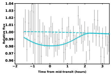
Figure 19: The Apr 2021 $g$’ transit data (grey points) was consistent with a non-detection or at least a significantly weaker transit. The model derived from the fit to all $g$’-band data are shown as a teal shaded region encompassing the uncertainties, and the GP without the transit is shown as a dashed line. The large uncertainties meant that this particular transit had a small weight.

Taken alone, the chromatic transit seen in the three data sets from 2021 Apr 24 suggests the transit-like signal is from a background or bound eclipsing binary where the eclipsing system is much redder than the source. However, this conclusion was strongly contradicted by our much more precise $g$’, $i$’, and $z_{s}$ transits from multiple other nights, which we used in our false-positive analysis (Section 6). No false-positive scenario can explain both a non-detection in $g$’ on Apr 24, and the clear detections on other nights, particularly since we have clear detections on both even and odd transits (see Table 1). A more likely explanation is that the 2021 Apr 24 transit was impacted by spots or flares.

Flares from the $\simeq$24 Myr M dwarf AU Mic have been known to distort, weaken, and nearly erase transits of the two planets, even at TESS wavelengths (Martioli et al., 2021; Gilbert et al., 2021). These effects should be much larger in $g^{\prime}$, which could explain why $z_{s}$ was not impacted significantly.

If the planet crosses a heavily spotted region, it will block less light than when crossing the warmer region. For such cool stars, small changes in $T_{\text{eff}}$ have a large effect on the blue end of the spectrum and a relatively small effect where the SED peaks (in $z_{s})$; the result is that modest spots can make a $g$’ transit extremely weak without impacting the $z_{s}$ transit. Such spot crossings can easily happen in one transit and not others, as the rotation period and orbital period are not harmonics of each other and spots on young M dwarfs are known to appear and disappear on month timescales (Rampalli et al., 2021).

To test this, we fit each of the three transits from 2021 Apr 24 individually, placing priors on the period, $T_{0}$, $b$, $\rho$, and limb-darkening. As we explain below, the GP kernel can fit out much of the discrepancy (i.e., a flexible GP can get the transits to match), so we did not use a GP model in this test. Instead, we fit a linear trend to the out-of-transit data. This is a conservative assumption, as it will make the errors on the transit depth smaller and hence harder to explain. Fitting for a spot in the transit would be challenging with the data, so we instead fit for the possible range of spots that could explain these depths following the basic methodology of Rackham et al. (2018), but forcing the transit to cross the spotted region rather than a pristine transit cord and a spotted star. There were three free parameters: the spot temperature ($T_{\rm{spot}}$), the fraction of the star that is spotted ($f_{S}$), and the transit depth had there been no spots ($D$). We restricted $5\%<f_{S}<80\%$, because smaller fractions would not be sufficient to fill the transit cord and larger would be noticeable as a change in $T_{\text{eff}}$ with wavelength (see Section 4 and Figure 11). The surface temperature was locked to the value from Section 4. The measurements were the three transit depths and the global fit depth (which only constrains $D$). We wrapped this in an MCMC framework using emcee, running for 50,000 steps with 50 walkers.

We show the resulting posterior in Figure 20. The spots could not be much cooler than 2700 K unless the spot coverage was $\gtrsim 60\%$ because colder spots would change the $z_{s}$ transit. Spot coverage fractions $>$60% are rare even in young stars (Morris, 2020), although not unheard of (e.g., Gully-Santiago et al., 2017). Such high fractions are also unlikely based on the stellar variability and spectrum. On the high end, the spot temperatures were limited by the stellar surface temperature. However, modest (5–30%) spot fractions consistent with expectations for young stars can explain all observations. Since spot temperatures close to the surface temperature are allowed, even moderate ($\gtrsim$30%) spot factions might not impact the spectroscopic analysis significantly (see Section 4 and Figure 11). We conclude that spots could easily explain the anomalous transit.

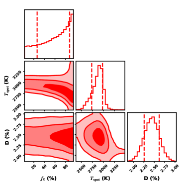
Figure 20: Corner plot of the posteriors from our transit+spot fit to the 2021 Apr 24 transit data for the spot parameters. The shaded regions correspond to 1-3$\sigma$ of the MCMC points and the dashed lines indicate the 1$\sigma$ interval. The constraints are the three transits ($g$, $Rc$, and $z_{s}$) as well as the overall depth from the global fit. The planet is assumed to be crossing a spotted region, which results in a weaker transit at bluer wavelengths. Although the fit favors a high spot fraction ($f_{S}>50\%$), this is unlikely given the stellar variability and wavelength-independent temperature. The region of the posterior with modest ($<30\%$) spot fractions and temperatures similar to the surface (3070 K) can fully explain the anomalous $g$-band transit and are consistent with all other observables.

As an additional test, we re-ran all $g$’ transit data through MISTTBORN. This was effectively a repeat of our analysis from Section 6 including the 2021 Apr 24 data; as in previous fits, a single GP was used to model stellar variability. The goal was to see if including this data could change our interpretation. The resulting transit depth was $2.27^{+0.33}_{-0.26}\%$, consistent with our earlier fits as well as the other $g$-band data (Figure 18). The depth change was insignificant because the SOAR $g$’-band data are far more precise, and significant stellar variability can explain a lot of the apparent discrepancy (which the GP can fit; see Figure 19). The updated depth was still sufficient to rule out all possible binaries from the MOLUSC analysis.

7 Why is TOI1227 b so big?

No Jovian-sized planets have been discovered around mid-to-late M dwarfs (Figure 21). Greater than 4$\,R_{\oplus}$ planets would have been easily detected in the (mid-)M dwarf samples covered by Kepler (Dressing & Charbonneau, 2015; Gaidos et al., 2016; Hardegree-Ullman et al., 2019) K2 (Dressing et al., 2017; Hardegree-Ullman et al., 2020), and ground-based surveys (e.g., MEarth; Berta et al., 2013), but such programs found only upper limits in this regime. The planet experiences stellar irradiance compared to most known planets, and should not be inflated. Instead, by $>$100 Myr we expect TOI 1227 b to more closely resemble the common sub-Neptunes seen around older stars. We explore this further below.

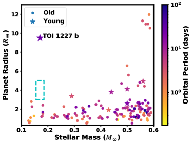
Figure 21: Planet radius as a function of host-star mass for transiting planets from the NASA exoplanet archive (NASA Exoplanet Science Institute, 2020). We denote systems around young stars ($<800$  Myr) with stars, as many planets in Hyades/Praesepe have abnormally large radii (Obermeier et al., 2016; Mann et al., 2017). All points are colored by their orbital period. The cyan region shows the likely final position of TOI 1227 b based on our MESA evolutionary models.

7.1 Evolutionary Modeling

To determine the possible current internal structure and future evolution of TOI 1227 b we compared its current properties to evolutionary models. We followed the framework of Owen (2020) where we constrained TOI 1227 b’s core mass, initial hydrogen dominated atmosphere mass fraction and initial (Kelvin-Helmholtz) cooling timescale to match its current age and radius. We considered planets with core masses $<$25 $M_{\oplus}$ and restricted ourselves to initial cooling timescales $<$1 Gyr and applied uniform priors in core-mass, log initial envelope mass fraction and log initial cooling timescale. The evolutionary tracks were computed using mesa (Paxton et al., 2011, 2013) and included mass-loss due to photoevaporation and irradiation from an evolving host star (Owen & Wu, 2013; Owen & Morton, 2016). The methodology also accounted for uncertainty in the protoplanetary disk dispersal timescale. Figure 22 shows the resulting marginalized probability distribution for core-mass and initial envelope mass fraction.

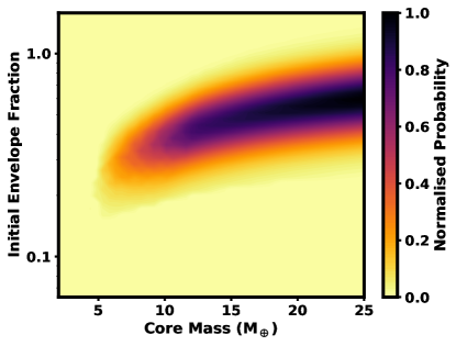
Figure 22: The marginalized probability distribution for TOI 1227 b’s core mass and initial hydrogen dominated envelope mass fraction that explains its current properties.

With initial envelope mass fractions $<$1, our results confirmed that TOI 1227 b is likely a young inflated planet that is actively cooling, eventually becoming one of the ubiquitous sub-Neptunes. We note the slight preference for higher core mass is likely artificial because the models with higher core masses are strongly biased towards longer initial cooling times. While we selected an upper limit of 1 Gyr in our modeling, this was likely an overestimate as the longest initial cooling timescales expected predicted by formation models that include an early “boil-off” phase are of order a few 100 Myr. However, our modeling indicated that core masses $\lesssim$5 $M_{\oplus}$ are strongly ruled out.

We followed the future evolutionary pathways of a subset of the model planets by selecting three representative cooling tracks and appropriate initial cooling timescales. These results are presented in Figure 23, showing that for plausible initial planet masses and initial cooling timescales they evolve into a sub-Neptune with a size 3–5 $R_{\oplus}$ at billion-year ages. Such planets are still rare around M dwarfs, but much more consistent with the locus of detections (Figure 21).

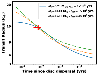
Figure 23: Possible evolutionary tracks for TOI 1227 b for a range of plausible initial masses ($M_{i}$) and cooling times ($t_{KH}$). These correspond to high (green) medium (orange) and low (blue) entropy. In choosing these evolutionary curves we have assumed the disk dispersed at a stellar age of 3 Myr. The red cross indicates the age and radius of TOI 1227 b, which are used as the observables on the model fit.

8 Summary and Discussion

TOI 1227 b is an $\simeq$11 Myr giant (0.85 $R_{J}$) planet orbiting a low-mass (0.17 $M_{\odot}$) M star in the LCC region of the Scorpius-Centarus OB association. Recent work on LCC has identified substructures, i.e. smaller populations, each with slightly different Galactic motion, position, and age. TOI 1227 b was flagged as a member of the A0 group by Goldman et al. (2018) and LCC-B by Kerr et al. (2021), which are effectively the same group. Because of the contradictory and easily forgotten naming, we denote this group Musca after the constellation containing most of the members.

As part of our effort to better measure the age of TOI 1227 b, we used rotation, lithium, and stellar evolution models to determine an age of 11$\pm$2 Myr for Musca, and hence TOI 1227 b. The young age placed TOI 1227 b as one of only two systems with transiting planets younger than 15 Myr (K2-33 b; Mann et al., 2016a; David et al., 2016), and one of only eleven transiting planets younger than 100 Myr (V1298 Tau, DS Tuc, AU Mic, TOI 837, HIP 67522, and TOI 942 David et al., 2019a; Newton et al., 2019; Benatti et al., 2019; Plavchan et al., 2020; Rizzuto et al., 2020; Bouma et al., 2020; Zhou et al., 2020; Carleo et al., 2021). Even including radial velocity detections only adds a few (Johns-Krull et al., 2016; Yu et al., 2017; Donati et al., 2017), some of which are still considered candidates (Donati et al., 2020; Damasso et al., 2020).

Like K2-33 b, TOI 1227 b is inflated, with a radius much larger than known transiting planets orbiting similar-mass stars (Figure 21). TOI 1227 b’s radius is closer to Jupiter than to the more common 1–3 $R_{\oplus}$ planets seen around mid-to-late M dwarfs (Berta et al., 2013; Hardegree-Ullman et al., 2019). Such a large planet would be obvious in surveys of older M dwarfs, especially given that the equivalent mature M dwarfs are both less variable and a factor of a few smaller than their pre-main-sequence counterparts. Thus, TOI 1227 b is evidence of significant radius evolution, especially when combined with similar earlier discoveries.

Interestingly, evolutionary models favor a final radius for TOI 1227 b of $>$3 $R_{\oplus}$, which would still be abnormally large (Figure 21) for the host star’s mass. However, that discrepancy is easier to explain as observational bias. Furthermore, the evolutionary tracks are poorly constrained by the existing young planet population, especially given that AU Mic b is the only $<$50 Myr planet with both mass and radius measurements (Klein et al., 2021; Cale et al., 2021). The lack of masses remains a significant challenge for these kinds of comparisons (Owen, 2020). TOI 1227 b is too faint for radial velocity follow-up in the optical, but might be within the reach of high-precision NIR monitoring. Our IGRINS monitoring achieved 40–50 m s^-1 precision, which is below the level from the stellar jitter. More dedicated monitoring and careful fitting of stellar and planetary signals should be able to detect a planet below $\simeq$40 $M_{\oplus}$.

A less challenging follow-up would be spin-orbit alignment through Rossiter-Mclaughlin, where the signal is expected to be $>$200 m s^-1 and the transit timescale ($\simeq$5 h) is much shorter than the rotational jitter (1.65 days). Recent measurements of stellar obliquity in young planetary systems have found that they are generally aligned with their host stars (e.g., Rodriguez et al., 2019; Zhou et al., 2020; Wirth et al., 2021), suggesting that these planets formed in situ or migrated through their protoplanetary disk. However, the number of misaligned systems even around older stars is $\lesssim$10% (varying with spectral type and planet mass; Fabrycky & Winn, 2009; Morton & Winn, 2014; Campante et al., 2016). We likely need a larger sample of obliquity measurements in young systems for a significant statistical comparison.

Follow-up and characterization of TOI 1227 b highlight the difficulties of characterizing and validating such young planets. We initially mischaracterized both the host star and planet, and ground-based transits yielded some contradictory results. The host star (TOI 1227) was initially thought to be part of the $\simeq$5 Myr $\epsilon$ Cha cluster, based on the BANYAN code. At that age, the stellar host would be even larger, yielding an even larger radius for the planet and creating a more complex set of false-positive scenarios (e.g., the planet radius would be more consistent with a young brown dwarf). Without Gaia, it is unlikely that Musca would have been recognized, and assigning TOI 1227 to a given population without a parallax would have been extremely challenging.

Similarly, the THYME team originally flagged TOI 1227 b as a likely eclipsing binary based on its V-shaped transit and large depth. Only with the SALT/HRS spectra and a consistent transit depth from Goodman/SOAR did we pursue further follow-up. This motivated both spectroscopic monitoring with IGRINS and the suite of multi-band transit photometry observed over $\simeq$1.5 years to better characterize the planet. While the majority of the transit photometry painted a clear picture that the signal was from a planet, a single transit showed an inconsistent transit depth, suggesting a false positive. We argued in Section 6.4 that regular flaring, the planet occulting spots, or simply low-precision photometry, could easily explain the unusual transit. Spots could also explain why our other $g$’ transits were deeper than the $i^{\prime}$ and $z_{s}$ data (Figure 18); if the transit cord has fewer spots than the rest of the stellar surface, the bluest transits appear deeper (this was seen in K2-25; Thao et al., 2020).

While the case for TOI 1227 b as a planet is strong, the initially confusing results raise concerns about the future follow-up of young planets. Radial velocity detection remains challenging. As with K2-25 b, the discovery transit for TOI 1227 b was V-shaped, making it hard to classify on transit depth and shape alone. Transits from young planets are likely to show some chromaticity even if the planet is real given the presence of spots, and smaller planets are not as amenable to the large suite of ground-based follow-up used here. Earlier studies often made use of Spitzer, which provided the advantage of a wide wavelength range while operating in a regime where the effects of spots and flares are significantly smaller. With the end of Spitzer, we may need to focus on improving the NIR photometric precision from the ground. For now, we encourage caution when rejecting young planets based on metrics tuned for older systems.

Table 5: Friends of TOI 1227

TIC	$\alpha$	$\delta$	RV	$\sigma_{\rm{RV}}$	RV	EqW Li	Li	$P_{\rm{rot}}$	Qual	CMG	SpyGlass	FF
	(J2016.0)	(J2016.0)	(km s-1)	(km s-1)	Source	mA	Source	(days)
360156606	186.76734	-72.45185	13.30	0.30	IGRINS	513	Goodman	1.65	Q0	Y	Y	Y
360003096	186.40895	-72.82357	$\ldots$	$\ldots$		598	Goodman	0.58	Q0	Y	Y	Y
360260204	187.87099	-72.83042	$\ldots$	$\ldots$		$\ldots$		10.22	Q3	Y	Y	Y
359697676	184.44271	-72.37392	$\ldots$	$\ldots$		382	Goodman	2.09	Q0	Y	Y	Y
360259773	187.57311	-72.98529	$\ldots$	$\ldots$		$\ldots$		6.53	Q1	Y	Y	Y
360331566	188.12874	-72.91861	$\ldots$	$\ldots$		479	Goodman	5.52	Q0	Y	Y	Y
360625930	189.85218	-72.73502	$\ldots$	$\ldots$		$\ldots$		6.60	Q0	Y	Y	Y
360259534	187.70690	-73.07898	$\ldots$	$\ldots$		563	Goodman	8.64	Q2	Y	Y	Y
326657935	188.45791	-71.42464	$\ldots$	$\ldots$		$\ldots$		1.61	Q0	N	Y	Y
359997243	186.21572	-72.60394	7.90	1.20	Kharchenko2007	23	ESO	2.99	Q1	Y	Y	Y
360906004	190.90566	-71.99760	$\ldots$	$\ldots$		$\ldots$		1.82	Q0	Y	Y	Y
360212499	187.32060	-73.91157	$\ldots$	$\ldots$		$\ldots$		0.47	Q3	N	Y	Y
359766629	185.15013	-73.88416	$\ldots$	$\ldots$		428	Goodman	2.91	Q0	Y	Y	Y
447994659	185.27027	-71.28040	14.30	0.45	Schneider2019	517	ESO	6.81	Q0	Y	Y	Y
360626787	189.65123	-73.02830	$\ldots$	$\ldots$		$\ldots$		4.92	Q2	N	N	Y
359851737	185.87389	-73.17399	$\ldots$	$\ldots$		$\ldots$		11.03	Q2	N	N	Y
359766954	184.93144	-74.06594	14.97	0.84	Schneider2019	558	ESO	6.75	Q0	Y	Y	Y
360627462	189.62496	-73.26625	$\ldots$	$\ldots$		439	Goodman	1.97	Q0	Y	Y	Y
359288962	182.61217	-72.11260	$\ldots$	$\ldots$		222	Goodman	2.38	Q0	Y	Y	Y
314231280	184.37701	-71.00238	$\ldots$	$\ldots$		$\ldots$		3.22	Q0	Y	Y	Y
359767456	184.97269	-74.33597	$\ldots$	$\ldots$		458	Goodman	10.22	Q0	Y	Y	Y
313853780	184.01031	-71.05102	$\ldots$	$\ldots$		$\ldots$		18.23	Q2	Y	Y	Y
454975214	179.87431	-72.64049	$\ldots$	$\ldots$		$\ldots$		0.47	Q0	N	Y	Y
360771943	190.48124	-73.18481	$\ldots$	$\ldots$		$\ldots$		1.26	Q0	N	Y	Y
328480578	190.73212	-70.57249	$\ldots$	$\ldots$		$\ldots$		1.01	Q0	N	Y	Y
313754471	184.10687	-71.39463	$\ldots$	$\ldots$		$\ldots$		1.51	Q0	Y	Y	Y
329538372	191.89997	-70.52056	$\ldots$	$\ldots$		$\ldots$		4.16	Q0	N	Y	Y
958526152	185.50216	-70.01776	$\ldots$	$\ldots$		$\ldots$		1.50	Q0	N	Y	Y
334999132	194.30115	-71.32633	$\ldots$	$\ldots$		$\ldots$		1.68	Q2	Y	Y	Y
360261300	187.60514	-72.43166	$\ldots$	$\ldots$		$\ldots$		1.03	Q0	Y	Y	Y
327147189	189.14024	-69.91816	$\ldots$	$\ldots$		$\ldots$		8.20	Q0	N	Y	Y
359357695	182.72617	-75.13193	$\ldots$	$\ldots$		515	Goodman	3.43	Q0	Y	Y	Y
360631514	189.83799	-75.04427	12.85	2.63	RAVEDR5	413	ESO	3.99	Q0	Y	Y	Y
328477573	190.55432	-69.73018	$\ldots$	$\ldots$		$\ldots$		0.72	Q0	N	Y	Y
327656671	189.69631	-71.66432	$\ldots$	$\ldots$		$\ldots$		6.29	Q0	Y	Y	Y
312803013	182.90841	-71.17671	13.50	0.10	Desidera2015	272	ESO	5.24	Q0	N	Y	Y
326542774	188.20581	-69.66814	$\ldots$	$\ldots$		$\ldots$		3.42	Q0	N	Y	Y
454980196	180.01050	-74.73522	$\ldots$	$\ldots$		$\ldots$		1.64	Q0	N	Y	Y
410981161	178.04938	-70.69887	$\ldots$	$\ldots$		$\ldots$		1.40	Q0	Y	Y	Y
361112047	191.97708	-75.42557	$\ldots$	$\ldots$		$\ldots$		0.33	Q0	Y	Y	Y
312803129	182.98363	-71.13739	$\ldots$	$\ldots$		$\ldots$		4.03	Q0	Y	Y	Y
359892714	185.70196	-74.17238	$\ldots$	$\ldots$		$\ldots$		0.47	Q0	Y	Y	Y
327665414	189.89608	-69.13804	$\ldots$	$\ldots$		445	Goodman	3.61	Q0	N	Y	Y
361392250	193.58588	-72.66762	$\ldots$	$\ldots$		$\ldots$		1.82	Q0	Y	Y	Y
405040121	185.59257	-71.61785	$\ldots$	$\ldots$		$\ldots$		0.83	Q0	N	Y	Y
327147732	189.28324	-69.77014	$\ldots$	$\ldots$		$\ldots$		1.42	Q3	N	N	Y
359573863	183.64167	-74.77805	$\ldots$	$\ldots$		$\ldots$		1.65	Q0	Y	Y	Y
360086059	186.49203	-75.85329	$\ldots$	$\ldots$		$\ldots$		1.28	Q0	N	Y	Y
454757744	175.87292	-74.31052	$\ldots$	$\ldots$		$\ldots$		1.92	Q0	Y	Y	Y
327549481	189.39036	-69.00110	$\ldots$	$\ldots$		$\ldots$		0.94	Q0	N	N	Y
328234948	190.21623	-68.94963	34.05	19.38	Gaia DR2	$\ldots$		3.00	Q0	N	Y	Y
326538701	188.35305	-68.81545	$\ldots$	$\ldots$		$\ldots$		1.66	Q0	N	Y	Y
311731608	181.28789	-70.07076	$\ldots$	$\ldots$		$\ldots$		9.57	Q0	N	Y	Y
334930665	194.03409	-69.44842	13.80	0.30	Torres2006	$\ldots$		4.59	Q0	N	N	Y
361113174	191.98801	-76.10258	$\ldots$	$\ldots$		$\ldots$		0.58	Q0	N	Y	Y
455000299	179.92537	-76.02397	12.63	1.40	Gaia DR2	460	ESO	7.90	Q0	N	Y	Y
297549461	180.65657	-69.19232	7.60	3.70	Kharchenko2007	25	ESO	0.30	Q1	Y	Y	Y
359000352	180.59159	-73.05367	$\ldots$	$\ldots$		358	Goodman	2.04	Q0	Y	Y	Y
454636797	173.52469	-72.87915	$\ldots$	$\ldots$		$\ldots$		4.38	Q1	N	N	Y
359065340	181.02908	-72.26877	$\ldots$	$\ldots$		$\ldots$		0.78	Q0	Y	Y	Y
454851844	177.68682	-74.18711	15.00	1.20	Murphy2013	404	ESO	1.06	Q0	N	N	Y
360899642	190.93459	-74.20175	$\ldots$	$\ldots$		$\ldots$		1.05	Q0	N	N	Y
410986249	178.32330	-71.14346	$\ldots$	$\ldots$		$\ldots$		1.75	Q0	Y	Y	Y
313865023	184.11613	-68.96561	$\ldots$	$\ldots$		$\ldots$		1.68	Q3	N	N	Y
359139846	181.37133	-76.01453	$\ldots$	$\ldots$		$\ldots$		0.42	Q3	Y	Y	Y
335376063	194.60605	-70.48039	9.60	0.90	Desidera2015	$\ldots$		2.00	Q0	N	N	Y
454541357	171.77052	-72.32937	$\ldots$	$\ldots$		$\ldots$		1.19	Q0	Y	Y	Y
327667179	189.67291	-68.76646	$\ldots$	$\ldots$		$\ldots$		0.79	Q0	Y	N	Y
361289085	193.06188	-76.47441	$\ldots$	$\ldots$		$\ldots$		1.87	Q0	N	Y	Y
334660676	193.77151	-68.75523	$\ldots$	$\ldots$		$\ldots$		1.70	Q0	N	N	Y
359571841	183.85674	-76.05843	$\ldots$	$\ldots$		$\ldots$		0.80	Q0	N	N	Y
959134031	191.49579	-68.14649	$\ldots$	$\ldots$		$\ldots$		4.75	Q2	N	N	Y
454718471	175.20625	-74.99425	10.30	1.00	Murphy2013	$\ldots$		0.50	Q0	Y	Y	Y
313174402	183.28939	-69.19817	$\ldots$	$\ldots$		$\ldots$		0.66	Q2	N	Y	Y
311374236	181.00944	-69.61571	$\ldots$	$\ldots$		$\ldots$		2.27	Q2	N	N	Y
327039106	188.81350	-70.71889	$\ldots$	$\ldots$		$\ldots$		24.56	Q2	N	N	Y
329454577	191.84103	-68.14453	3.03	2.49	RAVEDR5	$\ldots$		3.66	Q0	N	N	Y
394908401	203.37566	-73.69372	$\ldots$	$\ldots$		$\ldots$		0.67	Q0	Y	Y	Y
335367096	194.54401	-68.41302	$\ldots$	$\ldots$		$\ldots$		0.73	Q0	N	N	Y
359144755	181.46321	-73.17935	$\ldots$	$\ldots$		$\ldots$		1.29	Q0	Y	Y	Y
281757097	186.29977	-67.36249	$\ldots$	$\ldots$		$\ldots$		1.05	Q0	N	N	Y
312197475	181.90714	-69.20425	$\ldots$	$\ldots$		$\ldots$		0.66	Q1	N	Y	Y
311974232	181.72372	-67.55967	$\ldots$	$\ldots$		$\ldots$		1.70	Q0	N	N	Y
312204205	181.90170	-70.92725	$\ldots$	$\ldots$		$\ldots$		0.39	Q1	Y	N	Y
314759973	184.94741	-68.39638	$\ldots$	$\ldots$		$\ldots$		2.81	Q0	N	N	Y
327667195	189.67779	-68.76370	7.20	1.20	Kharchenko2007	67	ESO	0.79	Q2	Y	N	Y
360154672	187.07901	-73.10969	14.55	1.15	Gaia DR2	$\ldots$		6.16	Q0	N	N	Y
405089321	185.49499	-67.91525	$\ldots$	$\ldots$		$\ldots$		4.69	Q0	N	N	Y
454611617	173.34613	-76.36925	$\ldots$	$\ldots$		$\ldots$		1.57	Q0	N	N	Y
358994080	180.72684	-77.31060	14.40	0.60	Malo2014	256	ESO	2.50	Q0	N	N	Y
326660816	188.69208	-70.32378	$\ldots$	$\ldots$		$\ldots$		1.51	Q0	N	N	Y
340221485	201.14607	-70.34068	$\ldots$	$\ldots$		$\ldots$		1.64	Q1	Y	N	Y
297460759	180.12239	-70.84458	$\ldots$	$\ldots$		$\ldots$		0.63	Q0	N	N	Y
313648837	183.72736	-68.26724	$\ldots$	$\ldots$		$\ldots$		1.31	Q2	N	N	Y
454335224	167.71655	-72.92027	$\ldots$	$\ldots$		$\ldots$		1.04	Q0	N	N	Y
907780433	178.85370	-69.07816	$\ldots$	$\ldots$		$\ldots$		1.05	Q1	Y	N	N
313857039	184.16726	-70.12676	13.87	0.54	Gaia DR2	$\ldots$		4.11	Q0	Y	N	N
454826793	177.17699	-73.62319	$\ldots$	$\ldots$		$\ldots$		1.16	Q0	Y	N	N
328706525	190.98583	-68.21051	$\ldots$	$\ldots$		$\ldots$		1.41	Q0	Y	N	N
341448790	203.04825	-71.79406	$\ldots$	$\ldots$		$\ldots$		5.30	Q0	Y	N	N
329457630	191.73068	-68.72506	$\ldots$	$\ldots$		$\ldots$		2.58	Q0	N	Y	N
328235910	190.46474	-68.74517	$\ldots$	$\ldots$		$\ldots$		1.42	Q0	N	Y	N
329162367	191.64321	-68.07945	11.27	0.79	Gaia DR2	$\ldots$		14.12	Q2	N	Y	N
328985850	191.19354	-68.21358	$\ldots$	$\ldots$		$\ldots$		0.91	Q1	N	Y	N
329162173	191.42380	-68.11292	12.04	0.94	Gaia DR2	$\ldots$		5.30	Q0	N	Y	N
359137193	181.14973	-77.52634	10.40	2.00	LopezMarti2013	420	ESO	4.87	Q0	N	Y	N
359484011	183.57172	-73.35947	$\ldots$	$\ldots$		$\ldots$		1.68	Q0	N	Y	N
410983415	178.01551	-71.54682	$\ldots$	$\ldots$		$\ldots$		1.35	Q2	N	Y	N

Note. — Reference code: Torres2006 = Torres et al. (2006), Kharchenko2007 = Kharchenko et al. (2007), Murphy2013 = Murphy et al. (2013), LopezMarti2013 = Lopez Martí et al. (2013), Malo2014 = Malo et al. (2014), RAVEDR5 = Kunder et al. (2017), Gaia DR2 = DR2 = Katz et al. (2019), Schneider2019 = Schneider et al. (2019), Desidera2015 = Desidera et al. (2015), IGRINS = this work.

Appendix A Isochronal ages using mixture models

Ages derived from direct comparison to theoretical evolutionary models are impacted by a wide range of systematics. Binaries, for example, make the association look younger; an effect that varies with stellar mass (Sullivan & Kraus, 2021). The effect can be mitigated by explicitly including binaries in their model likelihood assuming an initial mass function and binary fraction (Kerr et al., 2021). This is less effective if the sample is biased towards or against binaries, which could easily arise from Gaia-based astrometry until later releases that account for binary motion. For young associations like those considered here, field interlopers (non-members) also bias the result towards older ages. Specific to populations like Musca is the presence of interlopers from other populations in LCC, which could bias the age in a direction that depends on the nearby populations.

Our solution is to fit the data with two populations simultaneously (a mixture model). The first population is the (ideally) single-age and single-star population of interest. The second is the ‘outlier’ population, which may contain nonmembers (field or nearby populations), binaries, stars with inaccurate photometry or parallaxes, or simply regions of the CMD that are poorly captured by the model grid. Following Hogg et al. (2010), the likelihood would be a sum of the two populations weighted by an amplitude:

$$\mathscr{L} \propto \prod_{i=1}^{N}\left[(1-P_{\mathrm{b}})P(\mathrm{interest})+P_{\mathrm{b}}\ P(\mathrm{outlier})\right]$$

$$\mathscr{L} \propto \prod_{i=1}^{N}\left[\frac{1-P_{\mathrm{b}}}{\sqrt{2\,\pi\,\sigma_{M_{x,i}}^{2}}}\,\exp\left(-\frac{[M_{x,i}-f(age,E(B-V),col_{i})]^{2}}{2\,\sigma_{M_{x,i}}^{2}}\right)\right.$$ (A1)

$$\quad\left.+\frac{P_{\mathrm{b}}}{\sqrt{2\,\pi\,[V_{\mathrm{b}}+\sigma_{M_{x,i}}^{2}]}}\,\exp\left(-\frac{[M_{x,i}-Y_{\mathrm{b}}]^{2}}{2\,[V_{\mathrm{b}}+\sigma_{M_{x,i}}^{2}]}\right)\right],$$

where $M_{x,i}$ is the absolute magnitude of the $i$th star in band $x$, $f(age,E(B-V),col_{i})$ is the predicted absolute magnitude from the model isochrones for a given age, reddening ($E(B-V)$), and color ($col_{i}$), and $\sigma_{M_{x,i}}$ is the total error in the star’s absolute magnitude and the propagated error from the star’s color. The parameters $P_{\mathrm{b}}$, $V_{\mathrm{b}}$, and $Y_{\mathrm{b}}$ are free parameters that describe the second population: the amplitude of the outliers (or the fraction of the population that are outliers), the mean absolute magnitude of the outliers, and the variance in the absolute magnitude of the outliers, respectively.

The simple likelihood above works well when most outliers are field M dwarfs, which are well described by a single Gaussian distribution in absolute magnitude versus color. However, we have both field and young interlopers that may occupy a large range of the CMD. Fortunately, such stars are still (mostly) restricted to the physically allowed regions of the CMD. Thus, we change the second term in the likelihood from a simple distribution in absolute magnitude to an offset from the population of interest:

$$\displaystyle P(\mathrm{outlier})=\frac{1}{\sqrt{2\,\pi\,[V_{\mathrm{b}}+\sigma_{M_{x,i}}^{2}]}}\,\exp\left(-\frac{[M_{x,i}-f(age,E(B-V),col_{i})-Y_{\mathrm{b}}]^{2}}{2\,[V_{\mathrm{b}}+\sigma_{M_{x,i}}^{2}]}\right).$$ (A2)

A downside of using an offset from the CMD to model the outliers is that the three outlier parameters can be biased by targets in regions of parameter space that are not well described by a simple offset, such as sources with poor parallaxes or M-dwarf white-dwarf binaries. This can be fixed by applying initial quality cuts. A more complicated problem is that the offset from the expected CMD likely varies with luminosity/mass, while we assumed a single parameter.

As a test, we ran our mixture model on the LCC-C (Crux-S) group and LCC-B groups from Kerr et al. (2021), which are similar cases to Musca. In both cases, we used the PARSECv1.2S isochrones (Bressan et al., 2012), assumed Solar metallicity, and cut out stars with RUWE$>$1.2. We restricted the comparison to Gaia magnitudes, as those were available for all stars, but tests adding in $JHK$ magnitudes yielded similar results. We show the resulting CMD and fit in Figure 24. For Crux-S, we derived an age of 12.6${}^{+1.6}_{-0.8}$ Myr, consistent with the 14.6$\pm$0.8 Myr from Kerr et al. (2021). For LCC-B, we estimated an age of 11.2${}^{+1.1}_{-0.8}$ Myr, consistent with 13.0$\pm$1.4 from Kerr et al. (2021). We also performed similar tests with older associations, such as MELANGE-1 from Tofflemire et al. (2021), which gave us an age of 210$\pm$70 Myr, an excellent match to the Li- and gyro-based ages ($250^{+50}_{-70}$ Myr) from Tofflemire et al. (2021).

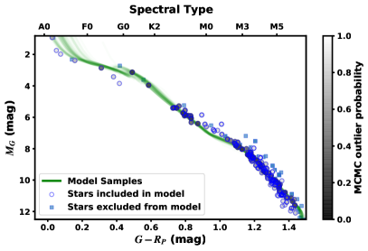
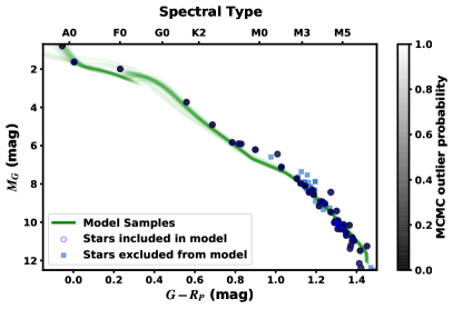
Figure 24: CMDs of the Crux-S (left) and LCC-B (right) groups from Kerr et al. (2021). Points including in our fit are labeled as blue circles, with blue squares representing stars excluded (mostly because of a high RUWE). Each point is shaded by the probability of being an outlier (i.e., not well-described by the model). This may include non-members, nearby association interlopers, binaries, or simply stars with poor parallaxes/photometry.

One advantage of the mixture model approach is the handling of regions where the models perform poorly. For example, in both test cases the PARSEC models fail to reproduce the population of M0-M2 dwarfs (Figure 24). Given that the magnetic models from DSEP better reproduce this region, it is likely that the offset is due to errors in the models as opposed to a high rate of binarity in that part of the selected population. In the case of LCC-C, there are few sources in that regime, so they have little effect on the overall age. For Crux-S, the mixture model weights these down in the fit.

However, the ability of this method to discard points is also a problem with this method; for Crux-S, the fit identifies many of the high-mass stars as medium-probability outliers, likely because it is challenging to fit the low-mass stars simultaneous with the high-mass ones (Feiden, 2016). A solution to this would be to run some systems with independent age estimates (such as from lithium depletion or traceback ages, Soderblom et al., 2014) to identify such systematics and apply corrections or weights. However, this requires a much more extensive set of associations with non-isochronal ages. A less elegant approach is to run the mixture code with multiple model grids.

Another drawback is when the population is poorly described by two models. However, the framework can be increased to explicitly model additional populations with sufficient terms. For example, one could use one term to handle the population of interest, a term to handle binaries with a prior or limits on the $Y_{\mathrm{b}}$-like term, and a term to model the (assumed) single-age population of young interlopers from other LCC groups. We found the simpler model to be sufficient for our purposes here, but hope to explore this in future iterations.

References

- Abe et al. (2013) Abe, L., Gonçalves, I., Agabi, A., et al. 2013, A&A, 553, A49, doi: 10.1051/0004-6361/201220351
- Aigrain et al. (2016) Aigrain, S., Parviainen, H., & Pope, B. J. S. 2016, MNRAS, 459, 2408, doi: 10.1093/mnras/stw706
- Alibert et al. (2005) Alibert, Y., Mordasini, C., Benz, W., & Winisdoerffer, C. 2005, A&A, 434, 343, doi: 10.1051/0004-6361:20042032
- Asplund et al. (2009) Asplund, M., Grevesse, N., Sauval, A. J., & Scott, P. 2009, ARA&A, 47, 481, doi: 10.1146/annurev.astro.46.060407.145222
- Baraffe et al. (2015) Baraffe, I., Homeier, D., Allard, F., & Chabrier, G. 2015, A&A, 577, A42, doi: 10.1051/0004-6361/201425481
- Bell et al. (2015) Bell, C. P. M., Mamajek, E. E., & Naylor, T. 2015, MNRAS, 454, 593, doi: 10.1093/mnras/stv1981
- Benatti et al. (2019) Benatti, S., Nardiello, D., Malavolta, L., et al. 2019, A&A, 630, A81, doi: 10.1051/0004-6361/201935598
- Berta et al. (2013) Berta, Z. K., Irwin, J., & Charbonneau, D. 2013, ApJ, 775, 91, doi: 10.1088/0004-637X/775/2/91
- Blackwell & Shallis (1977) Blackwell, D. E., & Shallis, M. J. 1977, MNRAS, 180, 177, doi: 10.1093/mnras/180.2.177
- Bonfils et al. (2013) Bonfils, X., Delfosse, X., Udry, S., et al. 2013, A&A, 549, A109, doi: 10.1051/0004-6361/201014704
- Bouma et al. (2020) Bouma, L. G., Hartman, J. D., Brahm, R., et al. 2020, The Astronomical Journal, 160, 239, doi: 10.3847/1538-3881/abb9ab
- Boyajian et al. (2012) Boyajian, T. S., von Braun, K., van Belle, G., et al. 2012, ApJ, 757, 112, doi: 10.1088/0004-637X/757/2/112
- Brandeker & Cataldi (2019) Brandeker, A., & Cataldi, G. 2019, A&A, 621, A86, doi: 10.1051/0004-6361/201834321
- Bressan et al. (2012) Bressan, A., Marigo, P., Girardi, L., et al. 2012, MNRAS, 427, 127, doi: 10.1111/j.1365-2966.2012.21948.x
- Brown et al. (2013) Brown, T. M., Baliber, N., Bianco, F. B., et al. 2013, PASP, 125, 1031, doi: 10.1086/673168
- Buckley et al. (2006) Buckley, D. A. H., Swart, G. P., & Meiring, J. G. 2006, in Society of Photo-Optical Instrumentation Engineers (SPIE) Conference Series, Vol. 6267, Society of Photo-Optical Instrumentation Engineers (SPIE) Conference Series, ed. L. M. Stepp, 62670Z
- Burt et al. (2020) Burt, J. A., Nielsen, L. D., Quinn, S. N., et al. 2020, AJ, 160, 153, doi: 10.3847/1538-3881/abac0c
- Cale et al. (2021) Cale, B., Reefe, M., Plavchan, P., et al. 2021, arXiv e-prints, arXiv:2109.13996. https://arxiv.org/abs/2109.13996
- Campante et al. (2016) Campante, T. L., Lund, M. N., Kuszlewicz, J. S., et al. 2016, The Astrophysical Journal, 819, 85, doi: 10.3847/0004-637x/819/1/85
- Cantat-Gaudin et al. (2018) Cantat-Gaudin, T., Jordi, C., Vallenari, A., et al. 2018, A&A, 618, A93, doi: 10.1051/0004-6361/201833476