Inverse medium scattering problems with Kalman filter techniques II. Nonlinear case

Abstract

In this paper, we study the inverse medium scattering problem to reconstruct unknown inhomogeneous medium from far field patterns of scattered waves. In the first part of our work, the linear inverse scattering problem was discussed, while in the second part, we deal with the nonlinear problem. The main idea is to apply the linear Kalman filter to the linearized problem. There are several ways to linearize, which introduce two reconstruction algorithms. Finally, we give numerical examples to demonstrate our proposed method.

Key words. Inverse acoustic scattering, Inhomogeneous medium, Far field pattern, Tikhonov regularization method, Kalman filter, Levenberg–Marquardt.

1 Introduction

The inverse scattering problem is the problem to determine unknown scatterers by measuring scattered waves that is generated by sending incident waves far away from scatterers. It is of importance for many applications, for example medical imaging, nondestructive testing, remote exploration, and geophysical prospecting. Due to many applications, the inverse scattering problem has been studied in various ways. For further readings, we refer to the following books [8, 9, 12, 28, 35], which include the summary of classical and recent progress of the inverse scattering problem.

We begin with the mathematical formulation of the scattering problem. Let $k>0$ be the wave number, and let $\theta\in\mathbb{S}^{1}$ be incident direction. We denote the incident field $u^{inc}(\cdot,\theta)$ with the direction $\theta$ by the plane wave of the form

$$u^{inc}(x,\theta):=\mathrm{e}^{ikx\cdot\theta},\ x\in\mathbb{R}^{2}.$$ (1.1)

Let $Q$ be a bounded domain and let its exterior $\mathbb{R}^{2}\setminus\overline{Q}$ be connected. We assume that $q\in L^{\infty}(\mathbb{R}^{2})$, which refers to the inhomogeneous medium, satisfies $\mathrm{Im}q\geq 0$, and its support $\mathrm{supp}\ q$ is embed into $Q$, that is $\mathrm{supp}\ q\Subset Q$. Then, the direct scattering problem is to determine the total field $u=u^{sca}+u^{inc}$ such that

$$\Delta u+k^{2}(1+q)u=0\ \mathrm{in}\ \mathbb{R}^{2},$$ (1.2)

$$\lim_{r\to\infty}\sqrt{r}\biggl{(}\frac{\partial u^{sca}}{\partial r}-iku^{sca}\biggr{)}=0,$$ (1.3)

where $r=|x|$. The Sommerfeld radiation condition (1.3) holds uniformly in all directions $\hat{x}:=\frac{x}{|x|}$. Furthermore, the problem (1.2)–(1.3) is equivalent to the Lippmann-Schwinger integral equation

$$u(x,\theta)=u^{inc}(x,\theta)+k^{2}\int_{Q}q(y)u(y,\theta)\Phi(x,y)dy,$$ (1.4)

where $\Phi(x,y)$ denotes the fundamental solution to Helmholtz equation in $\mathbb{R}^{2}$, that is,

$$\Phi(x,y):=\displaystyle\frac{i}{4}H^{(1)}_{0}(k|x-y|),\ x\neq y,$$ (1.5)

where $H^{(1)}_{0}$ is the Hankel function of the first kind of order one. It is well known that there exists a unique solution $u^{sca}$ of the problem (1.2)–(1.3), and it has the following asymptotic behaviour,

$$u^{sca}(x,\theta)=\frac{\mathrm{e}^{ikr}}{\sqrt{r}}\Bigl{\{}u^{\infty}(\hat{x},\theta)+O\bigl{(}1/r\bigr{)}\Bigr{\}},\ r\to\infty,\ \ \hat{x}:=\frac{x}{|x|}.$$ (1.6)

The function $u^{\infty}$ is called the far field pattern of $u^{sca}$, and it has the form

$$u^{\infty}(\hat{x},\theta)=\frac{k^{2}}{4\pi}\int_{Q}\mathrm{e}^{-ik\hat{x}\cdot y}u(y,\theta)q(y)dy=:\mathcal{F}_{\theta}q(\hat{x}),$$ (1.7)

where the far field mapping $\mathcal{F}_{\theta}:L^{2}(Q)\to L^{2}(\mathbb{S}^{1})$ is defined in the second equality for each incident direction $\theta\in\mathbb{S}^{1}$. For further details of these direct scattering problems, we refer to Chapter 8 of [12].

We consider the inverse scattering problem to reconstruct the function $q$ from the far field pattern $u^{\infty}(\hat{x},\theta_{n})$ for all directions $\hat{x}\in\mathbb{S}^{1}$ and several directions $\{\theta_{n}\}_{n=1}^{N}\subset\mathbb{S}^{1}$ with some $N\in\mathbb{N}$, and one fixed wave number $k>0$. It is well known that the function $q$ is uniquely determined from the far field pattern $u^{\infty}(\hat{x},\theta)$ for all $\hat{x},\theta\in\mathbb{S}^{1}$ and one fixed $k>0$ (see, e.g., [7, 37, 40]), but the uniqueness for several incident plane wave is an open question. For impenetrable obstacle scattering case, if we assume that the shape of scatterer is a polyhedron or ball, then the uniqueness for a single incident plane wave is proved (see [2, 10, 33, 32]). Recently in [1], they showed the Lipschitz stability for inverse medium scattering with finite measurements $\{u^{\infty}(\hat{x}_{i},\theta_{j})\}_{i,j=1,...,N}$ for large $N\in\mathbb{N}$ under the assumption that the true function belongs to a compact and convex subset of finite-dimensional subspace.

Our problem for equation (1.7) with finite measurements $\{u^{\infty}(\cdot,\theta_{n})\}_{n=1}^{N}$ is not only ill-posed, but also nonlinear, that is, the far field mappings $\mathcal{F}_{\theta}$ is nonlinear because $u(\cdot,\theta)$ in (1.7) is a solution for the Lippmann-Schwinger integral equation (1.4), which depends on $q$. Existing methods for solving nonlinear inverse problem can be roughly categorized into two groups: iterative optimization methods and qualitative methods. The iterative optimization method (see e.g., [3, 12, 15, 20, 27]) does not require many measurements, however it require the initial guess which is the starting point of the iteration. It must be appropriately chosen by a priori knowledge of the unknown function $q$, otherwise, the iterative solution could not converge to the true function. On the other hand, the qualitative method such as the linear sampling method [11], the no-response test [21], the probe method [22], the factorization method [29], and the singular sources method [39], does not require the initial guess and it is computationally faster than the iterative method. However, the disadvantage of the qualitative method is to require uncountable many measurements. For the survey of the qualitative method, we refer to [35]. Recently in [23, 34], they suggested the reconstruction method from a single incident plane wave although the rigorous justifications are lacked.

The well known method to solve the nonlinear problem is the Newton Method (see e.g., [3, 12, 27, 28, 31, 35]), which is a classical method to construct an iterative solution based on the first-order linearization. A natural approach applying the Newton method to our situation is to put all available measurements $\{u^{\infty}(\cdot,\theta_{n})\}_{n=1}^{N}$ and all far field mappings $\{\mathcal{F}_{\theta_{n}}\}_{n=1}^{N}$ into one long vectors $\vec{u}^{\infty}$ and $\vec{\mathcal{F}}$, respectively, and to iteratively solve the linearized big system of $\vec{u}^{\infty}=\vec{\mathcal{F}}q$ by the Tikhonov regularization, in other words to apply Levenberg–Marquardt scheme to $\vec{u}^{\infty}=\vec{\mathcal{F}}q$. However, this is computationally expensive when the number $N$ of measurements is increasing in which we have to construct the bigger system.

In this paper, we propose the reconstruction scheme based on the Kalman filter. The Kalman filter (see the original paper [26]) is the algorithm to estimate the unknown state in the dynamics system by using the time sequential measurements. The contributions of this paper are followings.

• We propose the reconstruction algorithm by combination of linearization and Kalman filter, which is equivalent to the Levenberg–Marquardt (see (4.13)–(4.17)).

• We also propose the reconstruction algorithm based on the Extended Kalman Filter (see (5.12)–(5.16)).

The algorithm in (A) is proposed by understanding the Levenberg–Marquardt scheme from the viewpoint of the Kalman filter, and the equivalence is proved by the first part of our work [14], which showed that the Kalman filter is equivalent to the Tikhonov regularization in the case of the linear inverse problem. The Extended Kalman filter (see e.g., [17, 16, 24]) is the nonlinear version of the Kalman filter, which idea is to linearize the nonlinear equation and update the state and weight every time to give one incident measurement. The algorithm in (B) is different from that in (A) in term of when to linearize the nonlinear equation, and the number of linearization in (B) is larger than that in (A). The figure 1 provides an illustration for the differences of (A) and (B). The advantages of using Kalman filter is that we do not require to construct the big system equation $\vec{u}^{\infty}=\vec{\mathcal{F}}q$, which reduces computational costs. Instead, we update not only state, but also the weight of the norm for the state space, which is associated with the update of the covariance matrices of the state in the statistical viewpoint (see Section 5 in [14]). Numerical experiments in Section 6 show that the reconstruction of (B) is robust to noise and its error decrease more rapidly rather than that of (A) although theoretical interpretations for this result is missing in this paper, which would be the focus of future work.

This paper is organized as follows. In Section 2, we recall the Fréchet derivative of the far field mapping $\mathcal{F}$ and its properties. In Section 3, we consider the linearized problem for nonlinear equation, and recall Levenberg–Marquardt method. In Section 4, we propose two reconstruction algorithms called the Full data Levenberg–Marquardt (FLM) and the Kalman filter Levenberg–Marquardt (KFL), and show that they are equivalent. In Section 5, we propose the reconstruction algorithm called the iterative Extended Kalman filter (EKF). Finally in Section 6, we give numerical examples to demonstrate our algorithms.

2 Fréchet derivative of the far field mapping

The approach for solving the nonlinear equation (1.7) often requires the linearization by the Fréchet derivative. In this section, we briefly recall the Fréchet derivative of the far field mapping and its properties. We denote by $L^{\infty}_{+}(Q):=\{q\in L^{\infty}(Q):\exists q_{0}>0,\ \mathrm{Im}q\geq q_{0}\ \mathrm{a.e}\ \mathrm{on}\ Q\}$.

We define the far filed mapping $\mathcal{F}_{\theta}:L^{\infty}_{+}(Q)\subset L^{2}(Q)\to L^{2}(\mathbb{S}^{1})$ by

$$\mathcal{F}_{\theta}q(\hat{x}):=\frac{k^{2}}{4\pi}\int_{Q}\mathrm{e}^{-ik\hat{x}\cdot y}u_{q}(y,\theta)q(y)dy=:u^{\infty}_{q}(\hat{x},\theta),\ \hat{x}\in\mathbb{S}^{1},$$ (2.1)

where the total field $u_{q}(\cdot,\theta)$ is given by the solving the integral equation of (1.4).

Lemma 2.1.

(1)

$\mathcal{F}_{\theta}\in C^{1}(L^{\infty}_{+}(Q),L^{2}(\mathbb{S}^{1}))$, that is, for any $q\in L^{\infty}_{+}(Q)$, $\mathcal{F}_{\theta}$ is Fréchet differentiable at $q$, and denoting the Fréchet derivative by $\mathcal{F}^{\prime}_{\theta}[q]:L^{2}(Q)\to L^{2}(\mathbb{S}^{1})$, the mapping $q\in L^{\infty}_{+}(Q)\mapsto\mathcal{F}^{\prime}_{\theta}[q]\in\mathcal{L}(L^{2}(Q),L^{2}(\mathbb{S}^{1}))$ is continuous, and its derivative $\mathcal{F}^{\prime}_{\theta}[q]$ at $q$ is given by

$$\mathcal{F}^{\prime}_{\theta}[q]m=v^{\infty}_{q,m},$$ (2.2)

where $v^{\infty}_{q,m}$ is the far field pattern of the radiating solution $v=v_{q,m}$ such that

$$\Delta v+k^{2}(1+q)v=-k^{2}mu_{q}(\cdot,\theta)\ \mathrm{in}\ \mathbb{R}^{2}.$$ (2.3)

(2)

$\mathcal{F}^{\prime}_{\theta}[\cdot]$ is locally bounded.

Proof.

First, we recall that from Lemmas 2.2, 2.3, 2.4, and 2.6 in [4], there exists $C_{1},...,C_{5}>0$ depending on $k$ and $Q$ such that

$$\left\|u_{q}(\cdot,\theta)\right\|_{L^{2}(Q)}\leq C_{1}(1+\left\|q\right\|_{L^{\infty}(Q)}),$$ (2.4)

$$\left\|u_{q_{1}}(\cdot,\theta)-u_{q_{2}}(\cdot,\theta)\right\|_{L^{2}(Q)}\leq C_{2}(1+\left\|q_{2}\right\|_{L^{\infty}(Q)})\left\|q_{1}-q_{2}\right\|_{L^{\infty}(Q)},$$ (2.5)

$$\left\|u_{q+m}(\cdot,\theta)-u_{q}(\cdot,\theta)-v_{q,m}(\cdot,\theta)\right\|_{L^{2}(Q)}\leq C_{3}(1+\left\|q\right\|_{L^{\infty}(Q)})\left\|m\right\|^{2}_{L^{\infty}(Q)},$$ (2.6)

$$\left\|v_{q,m}(\cdot,\theta)\right\|_{L^{2}(Q)}\leq C_{4}(1+\left\|q\right\|_{L^{\infty}(Q)})\left\|m\right\|_{L^{\infty}(Q)},$$ (2.7)

$$\left\|v_{q_{1},m}(\cdot,\theta)-v_{q_{2},m}(\cdot,\theta)\right\|_{L^{2}(Q)}\leq C_{5}(1+\left\|q_{2}\right\|_{L^{\infty}(Q)})\left\|q_{1}-q_{2}\right\|_{L^{\infty}(Q)}\left\|m\right\|_{L^{\infty}(Q)}.$$ (2.8)

(1) Concerning Fréchet differentiability, by using (2.5) and (2.6)

$$\begin{split}&\left|u^{\infty}_{q+m}(\hat{x},\theta)-u^{\infty}_{q}(\hat{x},\theta)-v^{\infty}_{q,m}(\hat{x},\theta)\right|\\ &\leq\left|\frac{k^{2}}{4\pi}\int_{Q}\left\{u_{q+m}(y,\theta)(q(y)-m(y))-u_{q}(y,\theta)q(y)-u_{q}(y,\theta)m(y)-v_{q,m}(y,\theta)q(y)\right\}dy\right|\\ &\leq C_{6}\big{\{}\left\|u_{q+m}(\cdot,\theta)-u_{q}(\cdot,\theta)\right\|_{L^{2}(Q)}\left\|m\right\|_{L^{\infty}(Q)}\\ &\hskip 113.81102pt+\left\|u_{q+m}(\cdot,\theta)-u_{q}(\cdot,\theta)-v_{q,m}(\cdot,\theta)\right\|_{L^{2}(Q)}\left\|q\right\|_{L^{\infty}(Q)}\big{\}}\\ &\leq C_{7}(1+\left\|q\right\|_{L^{\infty}(Q)})\left\|m\right\|^{2}_{L^{\infty}(Q)}.\end{split}$$ (2.9)

Concerning the continuity of the derivative, by using (2.5), (2.7), and (2.8)

$$\begin{split}&\left|v^{\infty}_{q_{1},m}(\hat{x},\theta)-v^{\infty}_{q_{2},m}(\hat{x},\theta)\right|\\ &\leq\left|\frac{k^{2}}{4\pi}\int_{Q}\left\{u_{q_{1}}(y,\theta)m(y)+v_{q_{1},m}(y,\theta)q_{1}(y)-u_{q_{2}}(y,\theta)m(y)-v_{q_{2},m}(y,\theta)q_{2}(y)\right\}dy\right|\\ &\leq C_{8}\big{\{}\left\|u_{q_{1}}(\cdot,\theta)-u_{q_{2}}(\cdot,\theta)\right\|_{L^{2}(Q)}\left\|m\right\|_{L^{\infty}(Q)}+\left\|v_{q_{1},m}\right\|_{L^{2}(Q)}\left\|q_{1}-q_{2}\right\|_{L^{\infty}(Q)}\\ &\hskip 113.81102pt+\left\|v_{q_{1},m}(\cdot,\theta)-v_{q_{2},m}(\cdot,\theta)\right\|_{L^{2}(Q)}\left\|q_{2}\right\|_{L^{\infty}(Q)}\big{\}}\\ &\leq C_{9}(1+\left\|q_{1}\right\|_{L^{\infty}(Q)}+\left\|q_{2}\right\|_{L^{\infty}(Q)})\left\|m\right\|_{L^{\infty}(Q)}\left\|q_{1}-q_{2}\right\|_{L^{\infty}(Q)}\end{split}$$ (2.10)

(2) Concerning the local boundedness, by using (2.4) and (2.7)

$$\begin{split}&\left|v^{\infty}_{q,m}(\hat{x},\theta)\right|\\ &\leq C_{10}\big{\{}\left\|u_{q}(\cdot,\theta)\right\|_{L^{2}(Q)}\left\|m\right\|_{L^{\infty}(Q)}+\left\|v_{q,m}\right\|_{L^{2}(Q)}\left\|q\right\|_{L^{\infty}(Q)}\big{\}}\\ &\leq C_{11}(1+\left\|q\right\|_{L^{\infty}(Q)})^{2}\left\|m\right\|_{L^{\infty}(Q)}\end{split}$$ (2.11)

∎

We observe the integral kernel of the linear operator $\mathcal{F}^{\prime}_{\theta}[q]$. The far field pattern $v^{\infty}=v^{\infty}(\cdot,\theta)$ is of the form

$$v^{\infty}_{q,m}(\hat{x},\theta)=\frac{k^{2}}{4\pi}\int_{Q}\mathrm{e}^{-ik\hat{x}\cdot y}\left[m(y)u_{q}(y,\theta)+q(y)v(y,\theta)\right]dy.$$ (2.12)

Here, we denote the fundamental solution for $-\Delta-k^{2}(1+q)$ by $\Phi_{q}(x,y)$, which is of the form

$$\Phi_{q}(x,y)=\Phi(x,y)+w(x,y),\ x\neq y,$$ (2.13)

where $w=w(\cdot,y)$ is the unique solution of the following integral equation

$$w(x,y)=k^{2}\int_{Q}\Phi(x,z)q(z)\left(w(z,y)+\Phi(z,y)\right)dz,\ x\in\mathbb{R}^{2}.$$ (2.14)

By using the fundamental solution $\Phi_{q}$, the radiating solution $v=v(\cdot,\theta)$ can be of the form

$$v(x,\theta)=k^{2}\int_{Q}\Phi_{q}(x,y)m(y)u_{q}(y,\theta)dy,\ x\in\mathbb{R}^{2}.$$ (2.15)

By combining (2.12) and (2.15), and using the Fubini’s theorem, we conclude that

$$\mathcal{F}^{\prime}_{\theta}[q]m(\hat{x})=\frac{k^{2}}{4\pi}\int_{Q}K_{q}(\hat{x},y)u_{q}(y,\theta)m(y)dy,\ \hat{x}\in\mathbb{S}^{1},$$ (2.16)

where the function $K_{q}$ is defined by

$$K_{q}(\hat{x},y):=\mathrm{e}^{-ik\hat{x}\cdot y}+k^{2}\int_{Q}\mathrm{e}^{-ik\hat{x}\cdot z}q(z)\Phi_{q}(z,y)dz.$$ (2.17)

We denote the far field mappings $\mathcal{F}:L^{\infty}_{+}(Q)\subset L^{2}(Q)\to L^{2}(\mathbb{S}^{1}\times\mathbb{S}^{1})$ by $\mathcal{F}q(\hat{x},\theta):=\mathcal{F}_{\theta}q(\hat{x})$, and from (2.9), the mapping $\mathcal{F}:L^{\infty}_{+}(Q)\to L^{2}(\mathbb{S}^{1}\times\mathbb{S}^{1})$ is also $C^{1}$. The following lemma is proved by the same argument in Section 11 of [12] and Section 2 of [4].

Lemma 2.2.

(1)

$\mathcal{F}:\{q\in L^{\infty}(Q):\mathrm{Im}q\geq 0\ \mathrm{a.e}\ \mathrm{on}\ Q\}\to L^{2}(\mathbb{S}^{1}\times\mathbb{S}^{1})$ is injective.

(2)

$\mathcal{F}\in C^{1}(L^{\infty}_{+}(Q),L^{2}(\mathbb{S}^{1}\times\mathbb{S}^{1}))$, and its derivative $\mathcal{F}^{\prime}[q]:L^{2}(Q)\to L^{2}(\mathbb{S}^{1}\times\mathbb{S}^{1})$ at $q$ is injective.

By Theorem 2.1 of [5], we have the following stability.

Lemma 2.3.

Let $W$ be a finite dimensional subspace of $L^{2}(Q)$, and Let $K$ be a compact and convex subset of $W\cap L^{\infty}_{+}(Q)$. Then, there exists a constant $C>0$ such that

$$\left\|q_{1}-q_{2}\right\|_{L^{2}(Q)}\leq C\left\|\mathcal{F}q_{1}-\mathcal{F}q_{2}\right\|_{L^{2}(\mathbb{S}^{1}\times\mathbb{S}^{1})},\ q_{1},q_{2}\in K.$$ (2.18)

Let $\{\theta_{i}:i\in\mathbb{N}\}$ be dense in $\mathbb{S}^{1}$. We denote $\vec{\mathcal{F}}_{N}:L^{2}(Q)\to L^{\infty}(\mathbb{S}^{1})^{N}$ by $\vec{\mathcal{F}}_{N}(q):=\left(\begin{array}[]{cc}\mathcal{F}_{\theta_{1}}q\\ \vdots\\ \mathcal{F}_{\theta_{N}}q\end{array}\right)$. Following lemma is proved by the same argument in Theorem 7 of [1].

Lemma 2.4.

Let $W$ be a finite dimensional subspace of $L^{2}(Q)$, and Let $K$ be a compact and convex subset of $W\cap L^{\infty}_{+}(Q)$. Then, for large $N\in\mathbb{N}$, there exists a constant $C_{N}>0$ such that

$$\left\|q_{1}-q_{2}\right\|_{L^{2}(Q)}\leq C_{N}\left\|\vec{\mathcal{F}}_{N}q_{1}-\vec{\mathcal{F}}_{N}q_{2}\right\|_{L^{2}(\mathbb{S}^{1})^{N}},\ q_{1},q_{2}\in K.$$ (2.19)

Proof.

We follow the proof of Theorem 7 of [1]. We first remark that the far-field patterns are analytic functions in $\mathbb{S}^{1}\times\mathbb{S}^{1}$. Since $\mathrm{dim}(\mathbb{S}^{1})=1$, and $1>\frac{1}{2}$, $H^{1}(\mathbb{S}^{1})$ is continuously embedded into $C(\mathbb{S}^{1})$, and so it is a reproducing kernel Hilbert space consisting of continuous functions. Let $P_{G_{N}}:H^{1}(\mathbb{S}^{1})\to H^{1}(\mathbb{S}^{1})$ be the projection onto $G_{N}$ defined by

$$G_{N}:=\mathrm{span}\{k_{\theta_{i}}:i=1,...,N\}$$ (2.20)

where the basis $k_{\theta_{i}}$ is unique solution of $f(\theta_{i})=\langle f,k_{\theta_{i}}\rangle_{H^{1}(\mathbb{S}^{1})}$. Then by Example 2 of [1], $P_{G_{N}}\to I_{H^{1}(\mathbb{S}^{1})}$ as $N\to\infty$ and

$$\left\|P_{G_{N}}f\right\|_{H^{1}(\mathbb{S}^{1})}\leq C_{N}\left\|(f(\theta_{1}),...,f(\theta_{N}))\right\|_{2}.$$ (2.21)

Let $P_{L^{2}(\mathbb{S}^{1};H^{1}(\mathbb{S}^{1}))}:L^{2}(\mathbb{S}^{1}\times\mathbb{S}^{1})\to L^{2}(\mathbb{S}^{1}\times\mathbb{S}^{1})$ be the projection onto the Bochner space $L^{2}(\mathbb{S}^{1};H^{1}(\mathbb{S}^{1}))\subset L^{2}(\mathbb{S}^{1}\times\mathbb{S}^{1})$. We define the bounded linear operator $Q_{N}:L^{2}(\mathbb{S}^{1}\times\mathbb{S}^{1})\to L^{2}(\mathbb{S}^{1}\times\mathbb{S}^{1})$ by $Q_{N}g(\hat{x},\theta)=P_{G_{N}}[P_{L^{2}(\mathbb{S}^{1};H^{1}(\mathbb{S}^{1}))}g(\hat{x},\cdot)](\theta)$. Then, $Q_{N}\big{|}_{L^{2}(\mathbb{S}^{1};H^{1}(\mathbb{S}^{1}))}\to I_{L^{2}(\mathbb{S}^{1};H^{1}(\mathbb{S}^{1}))}$. By Lemmas 2.1 and 2.3, we can apply Theorem 2 of [1] (as $T=L^{2}(\mathbb{S}^{1}\times\mathbb{S}^{1})$, $\tilde{Y}=L^{2}(\mathbb{S}^{1};H^{1}(\mathbb{S}^{1}))$ ), which implies that there exists a large $N\in\mathbb{N}$ such that by using (2.21)

$$\begin{split}&\left\|q_{1}-q_{2}\right\|\leq C\left\|Q_{N}u^{\infty}_{q_{1}}-Q_{N}u^{\infty}_{q_{2}}\right\|_{L^{2}(\mathbb{S}^{1}\times\mathbb{S}^{1})}\leq C\left\|P_{G_{N}}u^{\infty}_{q_{1}}-P_{G_{N}}u^{\infty}_{q_{2}}\right\|_{L^{2}(\mathbb{S}^{1};H^{1}(\mathbb{S}^{1}))}\\ &=C\left\{\int_{\mathbb{S}^{1}}\left\|P_{G_{N}}[u^{\infty}_{q_{1}}(\hat{x},\cdot)]-P_{G_{N}}[u^{\infty}_{q_{2}}(\hat{x},\cdot)]\right\|^{2}_{H^{1}(\mathbb{S}^{1})}ds(\hat{x})\right\}^{1/2}\\ &\leq C_{N}\left\{\sum_{i=1}^{N}\int_{\mathbb{S}^{1}}\left|u^{\infty}_{q_{1}}(\hat{x},\theta_{i})-u^{\infty}_{q_{2}}(\hat{x},\theta_{i})\right|^{2}ds(\hat{x})\right\}^{1/2}\leq C_{N}\left\|\vec{\mathcal{F}}_{N}q_{1}-\vec{\mathcal{F}}_{N}q_{2}\right\|_{L^{2}(\mathbb{S}^{1})^{N}}\end{split}$$ (2.22)

for $q_{1},q_{2}\in K$. ∎

3 Linearized problems

In this section, we consider the linearized problem for nonlinear equation, and recall Levenberg–Marquardt method. Let $X$ and $Y$ be Hilbert spaces over complex variables $\mathbb{C}$ which correspond to the state space $L^{2}(Q)$ of the inhomogeneous medium function $q$, and the observation space $L^{2}(\mathbb{S}^{1})$ of the far field pattern $u^{\infty}$, respectively. Let $A:X\to Y$ be a nonlinear observation operator which corresponds to the far field mapping $\mathcal{F}$.

For give $f\in Y$, we seek the solution $\varphi\in X$ such that

$$A(\varphi)=f.$$ (3.1)

We assume that we have an initial guess $\varphi_{0}\in X$, which is a starting point of the algorithm, and is appropriately determined by a priori information of the true solution $\varphi^{true}$ of (3.1). We also assume that the nonlinear mapping $A$ is Fréchet differentiable at $\varphi_{0}$, which implies that

$$A(\varphi)=A(\varphi_{0})+A^{\prime}[\varphi_{0}](\varphi-\varphi_{0})+r(\varphi-\varphi_{0}),$$ (3.2)

where the linear bounded operator $A^{\prime}[\varphi_{0}]:X\to Y$ is the Fréchet derivative of the nonlinear mapping $A$ at $\varphi_{0}$, and $r:X\to Y$ is some mapping corresponding to the remainder term such that $r(h)=o(h)$ as $\left\|h\right\|\to 0$. In the case to seek the solution $\varphi$ close to the initial guess $\varphi_{0}$, we can omit the remainder term $r$ because its influence is small. Then, we have the following linearized problem of (3.1).

$$A^{\prime}[\varphi_{0}](\varphi-\varphi_{0})=f-A(\varphi_{0}).$$ (3.3)

Although the problem become linear, the equation (3.3) may be ill-posed because the Fréchet derivative $A^{\prime}[\varphi_{0}]$ of $A$ is not generally invertible. Then, by the regularization method (see e.g., Chapter 4 of [12] and Chapter 3 of [35]), we have the regularized solution $\varphi_{\alpha}$ of (3.3)

$$\varphi_{\alpha}:=\varphi_{0}+\left(\alpha I+A^{\prime}[\varphi_{0}]^{*}A^{\prime}[\varphi_{0}]\right)^{-1}A^{\prime}[\varphi_{0}]^{*}\left(f-A(\varphi_{0})\right),$$ (3.4)

where $\alpha>0$ is a regularization parameter. Furthermore, we have an iterative algorithm for $i\in\mathbb{N}_{0}$

$$\varphi_{i+1}=\varphi_{i}+\left(\alpha_{i}I+A^{\prime}[\varphi_{i}]^{*}A^{\prime}[\varphi_{i}]\right)^{-1}A^{\prime}[\varphi_{i}]^{*}\left(f-A(\varphi_{i})\right),$$ (3.5)

which is known as the Levenberg–Marquardt method (see e.g., [19, 27]). So far, many type of the Newton method have been studied, for example, the regularized Gauss–Newton method (see e.g.,[3]) and the Quasi–Newton method (see e.g., [36]), and for any other, we refer to [20, 27, 38, 43]. We remark that the regularization parameter $\alpha_{i}>0$ in (3.5) is chosen such that the morozov discrepancy principle:

$$\left\|f-A(\varphi_{i})-A^{\prime}[\varphi_{i}](\varphi_{i+1}(\alpha)-\varphi_{i})\right\|=\rho\left\|f-A(\varphi_{i})\right\|,$$ (3.6)

with some fixed $\rho\in(0,1)$, where $\varphi_{i+1}(\alpha)$ is defined as in (3.5) replacing $\alpha_{i}$ by $\alpha$. Following lemma is the convergence.

Lemma 3.1 (Theorem 4.2 of [27], or Theorem 2.2 of [19]).

Let $0<\rho<1$ and assume that (3.1) is solvable in $B_{r}(\varphi_{0})$ where $r>0$ is some constant, and let $\varphi^{{\dagger}}\in B_{r}(\varphi_{0})$ be its solution, i.e., $f=A(\varphi^{{\dagger}})$, and assume that $A^{\prime}[\cdot]$ is uniformly bounded in $B_{r}(\varphi_{0})$, and a tangential cone condition: there exists $C>0$ such that for $\varphi,\widetilde{\varphi}\in B_{2r}(\varphi_{0})$

$$\left\|A(\varphi)-A(\widetilde{\varphi})-A^{\prime}[\varphi](\varphi-\widetilde{\varphi})\right\|\leq C\left\|\varphi-\widetilde{\varphi}\right\|\left\|A(\varphi)-A(\widetilde{\varphi})\right\|.$$ (3.7)

Then, if $\left\|\varphi_{0}-\varphi^{{\dagger}}\right\|<\rho/C$, then the Levenberg–Marquardt method $\varphi_{i}$ with $\{\alpha_{i}\}$ determined from (3.6) converges to a solution of $f=A(\varphi)$ as $i\to\infty$.

4 Levenberg–Marquardt and Kalman filter

The natural approach for solving the equation (1.7) is to put all available measurements $\{u^{\infty}_{n}\}_{n=1}^{N}$ and all far field mappings $\{\mathcal{F}_{n}\}_{n=1}^{N}$ where the index $n$ is associated with the incident direction $\theta_{n}\in\mathbb{S}^{1}$ into one long vector $\vec{u}^{\infty}$ and $\vec{\mathcal{F}}$, respectively, and to employ the Levenberg–Marquardt method (3.5) discussed in the Section 3. In order to study the above general situation, let $f_{1},...,f_{N}\in Y$ be measurements, let $A_{1},...,A_{N}$ be nonlinear observation operators, and let us consider the problem to determine $\varphi\in X$ such that

$$\vec{A}(\varphi)=\vec{f},$$ (4.1)

where $\vec{f}:=\left(\begin{array}[]{cc}f_{1}\\ \vdots\\ f_{N}\end{array}\right)$, and $\vec{A}(\varphi):=\left(\begin{array}[]{cc}A_{1}(\varphi)\\ \vdots\\ A_{N}(\varphi)\end{array}\right)$. By applying the Levenberg–Marquardt method (3.5) to the above system (4.1), we have iterative solution

$$\varphi^{FLM}_{i+1}:=\varphi^{FLM}_{i}+\left(\alpha_{i}I+\vec{A}^{\prime}[\varphi^{FLM}_{i}]^{*}\vec{A}^{\prime}[\varphi^{FLM}_{i}]\right)^{-1}\vec{A}^{\prime}[\varphi^{FLM}_{i}]^{*}\left(\vec{f}-\vec{A}(\varphi^{FLM}_{i})\right),$$ (4.2)

where $\varphi^{FLM}_{0}:=\varphi_{0}$, and $\vec{A}^{\prime}[\varphi]$ is denoted by $\vec{A}^{\prime}[\varphi]=\left(\begin{array}[]{cc}A^{\prime}_{1}[\varphi]\\ \vdots\\ A^{\prime}_{N}[\varphi]\end{array}\right)$, and the regularization parameters $\alpha_{i}>0$ satisfies the morozov discrepancy principle (3.6). We call this the Full data Levenberg–Marquardt. Here, $\vec{A}^{\prime}[\varphi_{0}]^{*}$ is a adjoint operator of $\vec{A}^{\prime}[\varphi_{0}]$ with respect to the usual scalar product $\langle\cdot,\cdot\rangle_{X}$ and the weighted scalar product $\langle\cdot,\cdot\rangle_{Y^{N},R^{-1}}:=\langle\cdot,R^{-1}\cdot\rangle_{Y^{N}}$ where $R:Y\to Y$ is the positive definite symmetric invertible operator, which is interpreted as the covariance matrices of the observation error distribution from a statistical viewpoint in the case when $X$ and $Y$ are Euclidean spaces (see Section 5 of [14]).

By the same calculation in (3.6) of [14], we have

$$\vec{A}^{\prime}[\varphi]^{*}=\vec{A}^{\prime}[\varphi]^{H}R^{-1},$$ (4.3)

where $\vec{A}^{\prime}[\varphi]^{H}$ is a adjoint operator of $\vec{A}^{\prime}[\varphi]$ with respect to usual scalar products $\langle\cdot,\cdot\rangle_{X}$ and $\langle\cdot,\cdot\rangle_{Y^{N}}$. Then, (4.2) can be of the form

$$\varphi^{FLM}_{i+1}=\varphi^{FLM}_{i}+\left(\alpha_{i}I+\vec{A}^{\prime}[\varphi^{FLM}_{i}]^{H}R^{-1}\vec{A}^{\prime}[\varphi^{FLM}_{i}]\right)^{-1}\vec{A}^{\prime}[\varphi^{FLM}_{i}]^{H}R^{-1}\left(\vec{f}-\vec{A}(\varphi^{FLM}_{i})\right),$$ (4.4)

Remark 4.1.

Let go back to our scattering problem, which $\vec{A}$ corresponds to the far field mapping $\vec{\mathcal{F}}$. From Lemma 2.2, $\vec{\mathcal{F}}$ is $C^{1}$, and its derivative is locally bounded. Furthermore, from Lemma 2.4, we have Lipschitz stability on compact convex subset of the finite dimensional subspace, which satisfies a tangential cone condition (3.7). Therefore by Lemma 3.1, our solution $q^{FLM}_{i}$ converges to true solution in the finite dimensional subspace if the initial geuss $q_{0}$ is very close to true one.

However, the algorithm (4.2) of the Full data Levenberg–Marquardt is computationally expensive when the number $N$ of measurements is increasing in which we have to construct the bigger system $\vec{A}\varphi=\vec{f}$. So, let us consider the alternative approach based on the Kalman filter. The Kalman filter is the linear estimation for the unknown state by the update of the state and its norm using the sequential measurements. For details of the following derivation, we refer to the first part of our works [14].

We consider the following problem for $n=1,...,N$

$$A^{\prime}_{n}[\varphi_{0}]\varphi=f_{n}-A_{n}(\varphi_{0})+A^{\prime}_{n}[\varphi_{0}]\varphi_{0},$$ (4.5)

which arises from the linearization of the problem $A_{n}(\varphi)=f_{n}$ at the initial guess $\varphi_{0}$. The above problem (4.5) can be applied to the Kalman filter algorithm (see (4.21)–(4.23) in [14]), then we obtain the following algorithm for $n=1,...,N$.

$$\varphi_{0,n}:=\varphi_{0,n-1}+K_{0,n}\left(f_{n}-A_{n}(\varphi_{0,0})+A^{\prime}_{n}[\varphi_{0,0}]\varphi_{0,0}-A^{\prime}_{n}[\varphi_{0,0}]\varphi_{0,n-1}\right),$$ (4.6)

$$K_{0,n}:=B_{0,n-1}A^{\prime}_{n}[\varphi_{0,0}]^{H}\left(R+A^{\prime}_{n}[\varphi_{0,0}]B_{0,n-1}A^{\prime}_{n}[\varphi_{0,0}]^{H}\right)^{-1},$$ (4.7)

$$B_{0,n}:=\left(I-K_{0,n}A^{\prime}_{n}[\varphi_{0,0}]^{H}\right)B_{0,n-1},$$ (4.8)

where $\varphi_{0,0}:=\varphi_{0}$, and $B_{0,0}:=\frac{1}{\alpha_{0}}I$. We denote the final state and covariance matrix in (4.6) and (4.8) by $\varphi_{1,0}:=\varphi_{0,N}$ and $B_{1,0}:=\frac{1}{\alpha_{1}}I$, which is the initial guess of the next iteration.

Next, we consider the following problem

$$A^{\prime}_{n}[\varphi_{1,0}]\varphi=f_{n}-A_{n}(\varphi_{1,0})+A^{\prime}_{n}[\varphi_{1,0}]\varphi_{1,0},$$ (4.9)

which arises from the linearization of the problem $A_{n}(\varphi)=f_{n}$ at $\varphi_{1,0}$. The above problem (4.9) can be applied to the Kalman filter algorithm as well, and we obtain the following algorithm for $n=1,...,N$.

$$\varphi_{1,n}:=\varphi_{1,n-1}+K_{1,n}\left(f_{n}-A_{n}(\varphi_{1,0})+A^{\prime}_{n}[\varphi_{1,0}]\varphi_{1,0}-A^{\prime}_{n}[\varphi_{1,0}]\varphi_{1,n-1}\right),$$ (4.10)

$$K_{0,n}:=B_{0,n-1}A^{\prime}_{n}[\varphi_{1,0}]^{H}\left(R+A^{\prime}_{n}[\varphi_{1,0}]B_{0,n-1}A^{\prime}_{n}[\varphi_{1,0}]^{H}\right)^{-1},$$ (4.11)

$$B_{0,n}:=\left(I-K_{0,n}A^{\prime}_{n}[\varphi_{1,0}]^{H}\right)B_{0,n-1},$$ (4.12)

We can repeat these procedure, then we obtain the following algorithm for $i\in\mathbb{N}_{0}$ and $n=1,...,N$

$$\varphi^{KFL}_{i,n}:=\varphi^{KFL}_{i,n-1}+K_{i,n}\left(f_{n}-A_{n}(\varphi^{KFL}_{i,0})+A^{\prime}_{n}[\varphi^{KFL}_{i,0}]\varphi^{KFL}_{i,0}-A^{\prime}_{n}[\varphi^{KFL}_{i,0}]\varphi^{KFL}_{i,n-1}\right),$$ (4.13)

$$K_{i,n}:=B_{i,n-1}A^{\prime}_{n}[\varphi^{KFL}_{i,0}]^{H}\left(R+A^{\prime}_{l}[\varphi^{KFL}_{i,0}]B_{i,n-1}A^{\prime}_{n}[\varphi^{KFL}_{i,0}]^{H}\right)^{-1},$$ (4.14)

$$B_{i,n}:=\left(I-K_{i,n}A^{\prime}_{n}[\varphi^{KFL}_{i,0}]^{H}\right)B_{i,n-1}.$$ (4.15)

When the iteration time $i$ is raised by one, the final state is renamed as

$$\varphi^{KFL}_{i,0}:=\varphi^{KFL}_{i-1,N},$$ (4.16)

and the weight is initialized as

$$B_{i,0}:=\frac{1}{\alpha_{i}}I,$$ (4.17)

where the regularization parameters $\alpha_{i}>0$ satisfies the morozov discrepancy principle (3.6). We call this the Kalman filter Levenberg–Marquardt. We remark that the algorithm has two indexes $i$ and $n$, where $i$ is associated with the iteration step, and $n$ measurement step, respectively.

Finally in this section, we show the following equivalent theorem, which is the nonlinear iteration version of Theorem 4.3 in [14].

Theorem 4.2.

For measurements $f_{1},...,f_{N}$, nonlinear mappings $A_{1},...,A_{N}$, and the initial guess $\varphi_{0}\in X$, and the initial regularization parameter $\alpha_{0}>0$, the Kalman filter Levenberg–Marquardt given by (4.13)–(4.17) is equivalent to the Full data Levenberg–Marquardt given by (4.4), that is, we have

$$\varphi^{KFL}_{i,N}=\varphi^{FLM}_{i+1},$$ (4.18)

for all $i\in\mathbb{N}_{0}$.

Proof.

We will prove (4.18) by the induction. By applying Theorem 4.3 of [14] to the linearized problem $A^{\prime}_{n}[\varphi_{0}]\varphi=f_{n}-A_{n}(\varphi_{0})+A^{\prime}_{n}[\varphi_{0}]\varphi_{0}$ for $n=1,...,N$ with the initial guess $\varphi_{0}$ and the regularization parameter $\alpha_{0}>0$, we have $\varphi^{KFL}_{0,N}=\varphi^{FLM}_{1}$, which is the case of $i=0$.

Let us assume that (4.18) in the case of $i-1$ holds, that is, we have $\varphi^{KFL}_{i-1,N}(=\varphi^{KFL}_{i,0})=\varphi^{FLM}_{i}=:\varphi_{i}$. Again, we apply Theorem 4.3 of [14] to the linearized problem $A^{\prime}_{n}[\varphi_{i}]\varphi=f_{n}-A_{n}(\varphi_{i})+A^{\prime}_{n}[\varphi_{i}]\varphi_{i}$ for $n=1,...,N$ with the initial guess $\varphi_{i}=\varphi^{KFL}_{i,0}=\varphi^{FLM}_{i}$ and the regularization parameter $\alpha_{i}>0$, then we have $\varphi^{KFL}_{i,N}=\varphi^{FLM}_{i+1}$. Theorem 4.2 has been shown. ∎

5 Iterative Extended Kalman filter

The usual Kalman filter is the linear optimal estimation for solving the linear system. However in realistic applications, most systems are nonlinear, so many studies of the nonlinear estimation have been done. The Extended Kalman filter, which is one of the nonlinear version of the Kalman filter, is to apply the linear Kalman filter to the linearized equation at the current state for every time to observe one measurement. For further readings of the Extended Kalman filter, we refer to [17, 16, 24], and there also exists other types of the nonlinear Kalman filter such as the Unscented Kalman Filter ([25]) which based on the Monte Carlo sampling without employing the linearization approximation. In this section, we introduce the algorithm based on the Extended Kalman filter.

First, let us start with the linearized problem of $A_{1}(\varphi)=f_{1}$ at the initial guess $\varphi_{0}$.

$$A^{\prime}_{1}[\varphi_{0}]\varphi=f_{1}-A(\varphi_{0})+A^{\prime}_{1}[\varphi_{0}]\varphi_{0}.$$ (5.1)

By the same argument in Section 4 of [14] replacing $A_{1}$ and $f_{1}$ by $A^{\prime}_{1}[\varphi_{0}]$ and $f_{1}-A(\varphi_{0})+A^{\prime}_{1}[\varphi_{0}]\varphi_{0}$, respectively, we have the following solution of (5.1).

$$\varphi_{1}:=\varphi_{0}+K_{1}\left(f_{1}-A_{1}(\varphi_{0})\right),$$ (5.2)

$$K_{1}:=B_{0}A^{\prime}_{1}[\varphi_{0}]^{H}\left(R+A^{\prime}_{1}[\varphi_{0}]B_{0}A^{\prime}_{1}[\varphi_{0}]^{H}\right)^{-1},$$ (5.3)

$$B_{1}:=\left(I-K_{1}A^{\prime}_{1}[\varphi_{0}]^{H}\right)B_{0},$$ (5.4)

where $B_{0}:=\frac{1}{\alpha_{0}}I$ and $\alpha_{0}>0$ is an initial regularization parameter.

Next, we consider linearized problem of $A_{2}(\varphi)=f_{2}$ at $\varphi_{1}$.

$$A^{\prime}_{2}[\varphi_{1}]\varphi=f_{2}-A_{2}(\varphi_{1})+A^{\prime}_{2}[\varphi_{1}]\varphi_{1},$$ (5.5)

Then, by the same argument in Section 4 of [14], we have the following solution of (5.5).

$$\varphi_{2}:=\varphi_{1}+K_{2}\left(f_{2}-A_{2}(\varphi_{1})\right),$$ (5.6)

$$K_{2}:=B_{1}A^{\prime}_{2}[\varphi_{1}]^{H}\left(R+A^{\prime}_{2}[\varphi_{1}]B_{2}A^{\prime}_{2}[\varphi_{1}]^{H}\right)^{-1},$$ (5.7)

$$B_{2}:=\left(I-K_{2}A^{\prime}_{2}[\varphi_{1}]^{H}\right)B_{1},$$ (5.8)

We can repeat them, then we have the following algorithm.

$$\varphi_{n}:=\varphi_{n-1}+K_{n}\left(f_{n}-A_{n}(\varphi_{n-1})\right),$$ (5.9)

$$K_{n}:=B_{n-1}A^{\prime}_{n}[\varphi_{n-1}]^{H}\left(R+A^{\prime}_{n}[\varphi_{n-1}]B_{n-1}A^{\prime}_{n}[\varphi_{n-1}]^{H}\right)^{-1},$$ (5.10)

$$B_{n}:=\left(I-K_{n}A^{\prime}_{n}[\varphi_{n-1}]^{H}\right)B_{n-1},$$ (5.11)

for $n=1,...,N$. In order to obtain the iterative algorithm, we repeat the arguments in the above (5.1)–(5.11) as the initial guess is $\varphi_{N}$. Finally, we obtain the following iterative algorithm for $i\in\mathbb{N}_{0}$ and $n=1,...,N$.

$$\varphi^{EKF}_{i,n}:=\varphi^{EKF}_{i,n-1}+K_{i,n}\left(f_{n}-A_{n}(\varphi^{EKF}_{i,n-1})\right),$$ (5.12)

$$K_{i,n}:=B_{i,n-1}A^{\prime}_{n}[\varphi^{EKF}_{i,n-1}]^{H}\left(R+A^{\prime}_{l}[\varphi^{EKF}_{i,n-1}]B_{i,n-1}A^{\prime}_{n}[\varphi^{EKF}_{i,n-1}]^{H}\right)^{-1},$$ (5.13)

$$B_{i,n}:=\left(I-K_{i,n}A^{\prime}_{n}[\varphi^{EKF}_{i,n-1}]^{H}\right)B_{i,n-1}.$$ (5.14)

When the iteration time $i$ is raised by one, the final state is renamed as

$$\varphi^{EKF}_{i,0}:=\varphi^{EKF}_{i-1,N},$$ (5.15)

and the weight as

$$B_{i,0}:=B_{i-1,N}.$$ (5.16)

We call this the iteratively Extended Kalman Filter. Figure 1 provides an illustration for the difference of Kalman filter Levenberg–Marquardt (KFL, left) and iterative Extended Kalman filter (EKF, right). When the state moves horizontally, measurements are used, and when it moves vertically, linearization are done. There are differences in term of when to linearize the nonlinear equation, and the number of linearization in EKF is larger than that in KFL.

Remark 5.1.

By Theorem 4.2, Kalman filter Levenberg–Marquardt (4.13)–(4.17) is equivalent to Full data Levenberg–Marquardt (4.4), which implies that in our scattering problem, Kalman filter Levenberg–Marquardt $q^{KFL}_{n,N}$ converges to the finite dimensional true solution (see Remark 4.1). Although we will not prove the rigorous convergence, iteratively Extended Kalman filter (5.12)-(5.16) could be expected to have the convergence because there exists several references [18, 6, 30], which discuss the convergence of Extended Kalman filter in the context of dynamic Kalman filter in the setting of the Euclidean space. They could be extended to our scattering setting, in particular to infinite dimensional Hilbert spaces over complex variable.

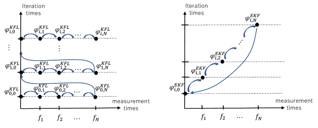
Figure 1: difference of KFL (left) and EKF (right)

6 Numerical examples

In this section, we provide numerical examples for the Kalman filter algorithm. Our inverse scattering problem is to solve the nonlinear integral equation

$$\mathcal{F}_{n}q=u^{\infty}(\cdot,\theta_{n}),$$ (6.1)

for $n=1,...,N$ where the operator $\mathcal{F}_{n}:L^{2}(Q)\to L^{\infty}(\mathbb{S}^{1})$ is defined by

$$\mathcal{F}_{n}q(\hat{x}):=\mathcal{F}q(\hat{x},\theta_{n}):=\frac{k^{2}}{4\pi}\int_{Q}\mathrm{e}^{-ik\hat{x}\cdot y}u_{q}(y,\theta_{n})q(y)dy,$$ (6.2)

where the incident direction is given by $\theta_{n}:=\left(\mathrm{cos}(2\pi n/N),\mathrm{sin}(2\pi n/N)\right)$ for each $n=1,...,N$. Here, $u_{q}(\cdot,\theta_{n})$ is the solution of Lippmann-Schwinger integral equation (1.4), which is numerically computed based on Vainikko’s method [41, 42], which is a fast solution method for the Lippmann–Schwinger equation based on periodization, fast Fourier transform techniques and multi-grid methods. We assume that the support of the function $q$ is included in $[-S,S]^{2}$ with some $S>0$. The linearized problem at $q$ of (6.1) is

$$\mathcal{F}^{\prime}_{n}[q_{0}](q-q_{0})=u^{\infty}_{n}-\mathcal{F}_{n}q_{0}+\mathcal{F}^{\prime}_{n}[q_{0}]q_{0},$$ (6.3)

where Fréchet derivative $\mathcal{F}^{\prime}_{l}[q_{0}]$ is of the form

$$\mathcal{F}^{\prime}_{n}[q_{0}]q(\hat{x})=\frac{k^{2}}{4\pi}\int_{Q}K_{q_{0}}(\hat{x},y)u_{q_{0}}(y,\theta_{n})q(y)dy,\ \hat{x}\in\mathbb{S}^{1}.$$ (6.4)

where $K_{q_{0}}(\hat{x},y)$ is defined by (2.16).

The linearized equation (6.3) is discretized by

$$\bm{\mathcal{F}^{\prime}_{n}[q_{0}]}\bm{q}=\bm{u^{\infty}_{n}}-\bm{\mathcal{F}_{n}q_{0}}+\bm{\mathcal{F}^{\prime}_{n}[q_{0}]q_{0}},$$ (6.5)

where

$$\bm{\mathcal{F}^{\prime}_{n}[q_{0}]}=\frac{k^{2}S^{2}}{4\pi M^{2}}\left(K_{q_{0}}(\hat{x}_{j},y_{m_{1},m_{2}})u_{q_{0}}(y_{m_{1},m_{2}},\theta_{n})\right)_{j=1,...,J,\ -M\leq m_{1},m_{2}\leq M-1}\in\mathbb{C}^{J\times(2M)^{2}}.$$ (6.6)

where $y_{m_{1},m_{2}}:=\left(\frac{(2m_{1}+1)S}{2M},\frac{(2m_{2}+1)S}{2M}\right)$, and $M\in\mathbb{N}$ is a number of the division of $[0,S]$ (i.e., the function $q$ is discretized by piecewise constant on $[-S,S]^{2}$ which is decomposed by squares with the length $\frac{S}{M}$), and $\hat{x}_{j}:=\left(\mathrm{cos}(2\pi j/J),\mathrm{sin}(2\pi j/J)\right)$, and $J\in\mathbb{N}$ is a number of the division of $[0,2\pi]$ and

$$\bm{q}=\left(q(y_{m_{1},m_{2}})\right)_{-M\leq m_{1},m_{2}\leq M-1}\in\mathbb{C}^{(2M)^{2}},$$ (6.7)

and

$$\bm{u_{n}^{\infty}}=\left(u^{\infty}(\hat{x}_{j},\theta_{n})\right)_{j=1,...,J}+\bm{\epsilon_{n}}\in\mathbb{C}^{J}.$$ (6.8)

The noise $\bm{\epsilon_{n}}\in\mathbb{C}^{J}$ is sampling from a complex Gaussian distribution $\mathcal{C}\mathcal{N}(0,\sigma^{2}\bm{I})$, which is equivalent to $\bm{\epsilon_{n}}=\bm{\epsilon^{re}_{n}}+i\bm{\epsilon^{im}_{n}}$ where $\bm{\epsilon^{re}_{n}},\bm{\epsilon^{im}_{n}}\in\mathbb{R}^{J}$ are independently identically distributed from $\mathcal{N}(0,\sigma^{2}\bm{I})$.

Here, we always fix discretization parameters as $J=30$, $M=8$, $S=3$, $N=30$, and weight $\bm{R}\in\mathbb{R}^{J\times J}$, which is the covariance matrix of the observation error distribution, as $R=r^{2}I$, and $r=3$.

We consider true functions as the characteristic function

$$q^{true}_{j}(x):=\left\{\begin{array}[]{ll}0.1&\quad\mbox{for $x\in B_{j}$}\\ 0&\quad\mbox{for $x\notin B_{j}$}\end{array}\right.,$$ (6.9)

where the support $B_{j}$ of the true function is considered as the following two types.

$$B_{1}:=\left\{(x_{1},x_{2}):x^{2}_{1}+x^{2}_{2}<1.5\right\},$$ (6.10)

$$B_{2}:=\left\{(x_{1},x_{2}):\begin{array}[]{cc}(x_{1}+1.5)^{2}+(x_{2}+1.5)^{2}<(1.0)^{2}\ or\\ 1<x_{1}<2,\ -2<x_{2}<2\ or\\ -2<x_{1}<2,\ -2.0<x_{2}<-1.0\end{array}\right\},$$ (6.11)

In Figure 2, the blue closed curve is the boundary $\partial B_{j}$ of the support $B_{j}$, and the green brightness indicates the value of the true function on each cell divided into $(2M)^{2}=256$ in the sampling domain $[-S,S]^{2}=[-3,3]^{2}$. Here, we always employ the initial guess $q_{0}$ as

$$q_{0}\equiv 0.$$ (6.12)

Figures 3 and 4 show the reconstruction by the Kalman filter Levenberg–Marquardt (KFL) discussed in (4.13)–(4.17) with noisy $\sigma=0.01$ and $0.1$, respectively, while Figures 5 and 6 show the reconstruction by and the iterative Extended Kalman filter (EKF) discussed in (5.12)–(5.16) with noisy $\sigma=0.01$ and $0.1$, respectively. The first and second columns in Figures 3 and 4 correspond to visualization for discrepancy constant $\rho=0.4$, and $0.8$, respectively, while those in Figures 5 and 6 correspond to visualization for initial regularization parameter $\alpha_{0}=50$, and $5$, respectively, for different two shapes $B_{1}$ and $B_{2}$, and for different two wave numbers $k=3$ and $k=7$. The third column corresponds to the graph of the Mean Square Error (MSE) defined by

$$e_{i}:=\left\|q^{true}-q_{i}\right\|^{2},$$ (6.13)

where $q_{i}$ is associated with the state of $i$th iteration step. The horizontal axis is with respect to number of iterations, and the vertical axis is the value of MSE. We observe that the error of Kalman filter Levenberg–Marquardt blows up in some case (wave number $k=3$ and noise $\sigma=0.1$), in which iterative Extended Kalman filter does not. We also obverse that the error of iterative Extended Kalman filter decreases more rapidly than that of Kalman filter Levenberg–Marquardt. Therefore, the result of iterative Extended Kalman filter is better than that of Kalman filter Levenberg–Marquardt in our experiments. It would be interesting to provide the ratio of convergence for two methods to justify these numerical experiments.

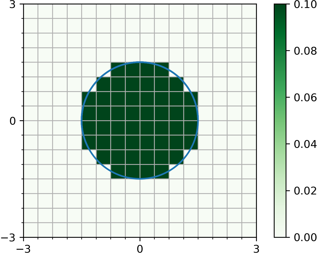
(a) $q^{true}_{1}$

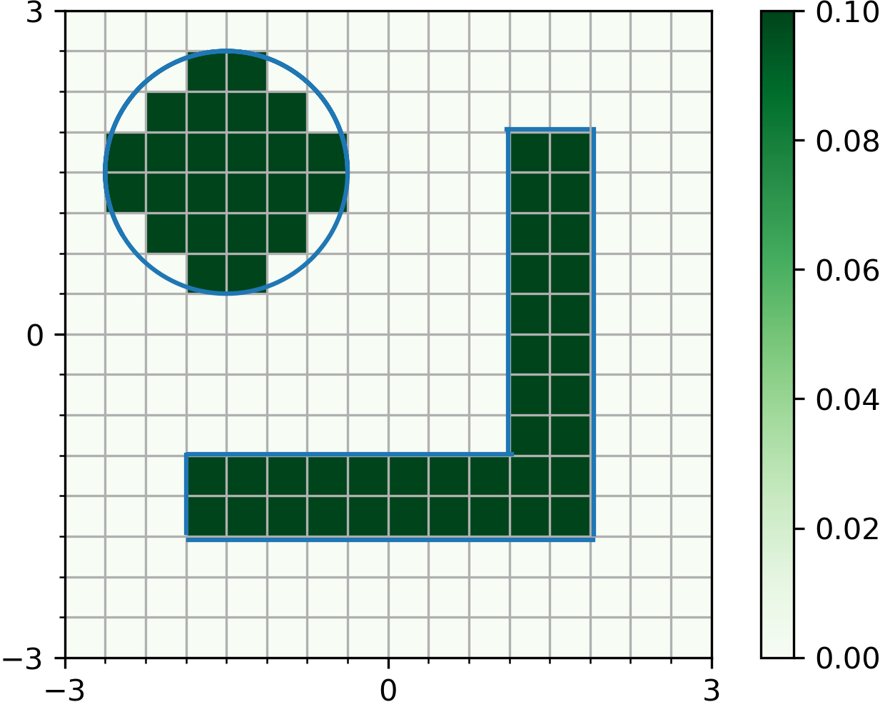
(b) $q^{true}_{2}$

Figure 2: true functions

(a) $B_{1}$, $k=3$, $\rho=0.4$ (b) $B_{1}$, $k=3$, $\rho=0.8$ (c) $B_{1}$, $k=3$, error graph

(d) $B_{1}$, $k=7$, $\rho=0.4$ (e) $B_{1}$, $k=7$, $\rho=0.8$ (f) $B_{1}$, $k=7$, error graph

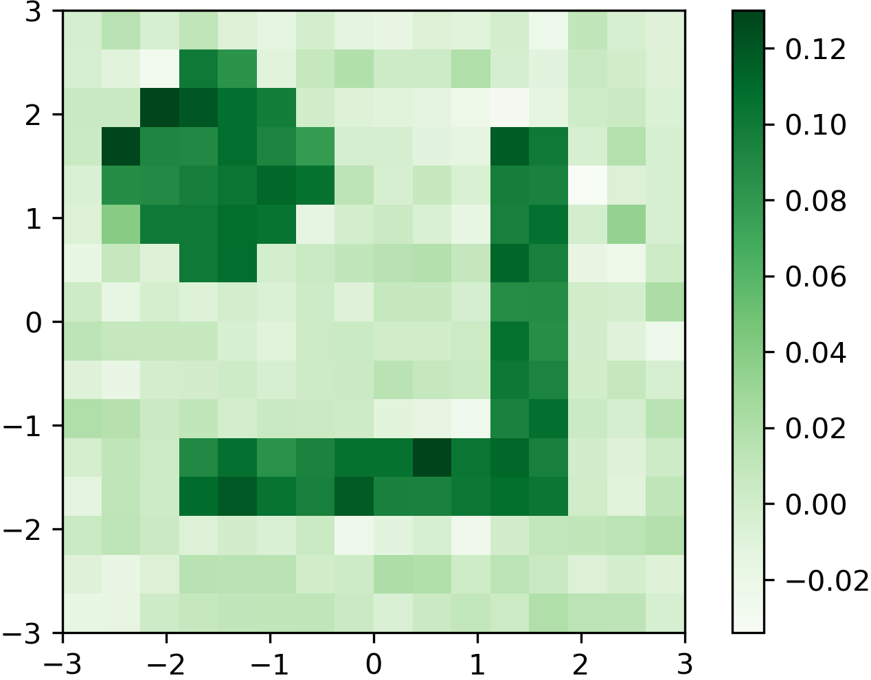
(g) $B_{2}$, $k=3$, $\rho=0.4$ (h) $B_{2}$, $k=3$, $\rho=0.8$ (i) $B_{2}$, $k=3$, error graph

(j) $B_{2}$, $k=7$, $\rho=0.4$ (k) $B_{2}$, $k=7$, $\rho=0.8$ (l) $B_{2}$, $k=7$, error graph

Figure 3: KFL (nosiy $\sigma=0.01$)

(a) $B_{1}$, $k=3$, $\rho=0.4$ (b) $B_{1}$, $k=3$, $\rho=0.8$ (c) $B_{1}$, $k=3$, error graph

(d) $B_{1}$, $k=7$, $\rho=0.4$ (e) $B_{1}$, $k=7$, $\rho=0.8$ (f) $B_{1}$, $k=7$, error graph

(g) $B_{2}$, $k=3$, $\rho=0.4$ (h) $B_{2}$, $k=3$, $\rho=0.8$ (i) $B_{2}$, $k=3$, error graph

(j) $B_{2}$, $k=7$, $\rho=0.4$ (k) $B_{2}$, $k=7$, $\rho=0.8$ (l) $B_{2}$, $k=7$, error graph

Figure 4: KFL (nosiy $\sigma=0.1$)

(a) $B_{1}$, $k=3$, $\alpha=50$ (b) $B_{1}$, $k=3$, $\alpha=5$ (c) $B_{1}$, $k=3$, error graph

(d) $B_{1}$, $k=7$, $\alpha=50$ (e) $B_{1}$, $k=7$, $\alpha=5$ (f) $B_{1}$, $k=7$, error graph

(g) $B_{2}$, $k=3$, $\alpha=50$ (h) $B_{2}$, $k=3$, $\alpha=5$ (i) $B_{2}$, $k=3$, error graph

(j) $B_{2}$, $k=7$, $\alpha=50$ (k) $B_{2}$, $k=7$, $\alpha=5$ (l) $B_{2}$, $k=7$, error graph

Figure 5: EKF (nosiy $\sigma=0.01$)

(a) $B_{1}$, $k=3$, $\alpha=50$ (b) $B_{1}$, $k=3$, $\alpha=5$ (c) $B_{1}$, $k=3$, error graph

(d) $B_{1}$, $k=7$, $\alpha=50$ (e) $B_{1}$, $k=7$, $\alpha=5$ (f) $B_{1}$, $k=7$, error graph

(g) $B_{2}$, $k=3$, $\alpha=50$ (h) $B_{2}$, $k=3$, $\alpha=5$ (i) $B_{2}$, $k=3$, error graph

(j) $B_{2}$, $k=7$, $\alpha=50$ (k) $B_{2}$, $k=7$, $\alpha=5$ (l) $B_{2}$, $k=7$, error graph

Figure 6: EKF (nosiy $\sigma=0.1$)

References

• [1] Giovanni S. Alberti and Matteo Santacesaria. Infinite-dimensional inverse problems with finite measurements, 2020.
• [2] Giovanni Alessandrini and Luca Rondi. Determining a sound-soft polyhedral scatterer by a single far-field measurement. Proceedings of the American Mathematical Society, 133(6):1685–1691, 2005.
• [3] Anatolii Borisovich Bakushinsky and M Yu Kokurin. Iterative methods for approximate solution of inverse problems, volume 577. Springer Science & Business Media, 2005.
• [4] G. Bao and Peijun Li. Inverse medium scattering for the helmholtz equation at fixed frequency. Inverse Problems, 21:1621–1641, 2005.
• [5] Laurent Bourgeois. A remark on lipschitz stability for inverse problems. Comptes Rendus Mathematique, 351(5):187–190, 2013.
• [6] M Boutayeb, H Rafaralahy, and M Darouach. Convergence analysis of the extended kalman filter as an observer for nonlinear discrete-time systems. In Proceedings of 1995 34th IEEE Conference on Decision and Control, volume 2, pages 1555–1560. IEEE, 1995.
• [7] Alexander L Bukhgeim. Recovering a potential from cauchy data in the two-dimensional case. 2008.
• [8] Fioralba Cakoni and David Colton. Qualitative methods in inverse scattering theory: An introduction. Springer Science & Business Media, 2005.
• [9] Xudong Chen. Computational methods for electromagnetic inverse scattering. John Wiley & Sons, 2018.
• [10] Jin Cheng and Masahiro Yamamoto. Uniqueness in an inverse scattering problem within non-trapping polygonal obstacles with at most two incoming waves. Inverse Problems, 19(6):1361, 2003.
• [11] David Colton and Andreas Kirsch. A simple method for solving inverse scattering problems in the resonance region. Inverse problems, 12(4):383, 1996.
• [12] David Colton and Rainer Kress. Inverse Acoustic and Electromagnetic Scattering Theory, volume 93. Springer Nature, 2019.
• [13] Melina A Freitag and Roland WE Potthast. Synergy of inverse problems and data assimilation techniques. In Large scale inverse problems, pages 1–54. De Gruyter, 2013.
• [14] Takashi Furuya and Roland Potthast. Inverse medium scattering problems with kalman filter techniques i. linear case. 2021.
• [15] Giovanni Giorgi, Massimo Brignone, Riccardo Aramini, and Michele Piana. Application of the inhomogeneous lippmann–schwinger equation to inverse scattering problems. SIAM Journal on Applied Mathematics, 73(1):212–231, 2013.
• [16] Mohinder S Grewal and Angus P Andrews. Applications of kalman filtering in aerospace 1960 to the present [historical perspectives]. IEEE Control Systems Magazine, 30(3):69–78, 2010.
• [17] Mohinder S Grewal and Angus P Andrews. Kalman filtering: Theory and Practice with MATLAB. John Wiley & Sons, 2014.
• [18] LZ Guo and QM Zhu. A fast convergent extended kalman observer for nonlinear discrete-time systems. International Journal of Systems Science, 33(13):1051–1058, 2002.
• [19] Martin Hanke. A regularizing levenberg - marquardt scheme, with applications to inverse groundwater filtration problems. Inverse Problems, 13(1):79–95, feb 1997.
• [20] Thorsten Hohage. On the numerical solution of a three-dimensional inverse medium scattering problem. Inverse Problems, 17(6):1743, 2001.
• [21] Naofumi Honda, Gen Nakamura, Roland Potthast, and Mourad Sini. The no-response approach and its relation to non-iterative methods for the inverse scattering. Annali di Matematica Pura ed Applicata, 187(1):7–37, 2008.
• [22] Masaru Ikehata. Reconstruction of an obstacle from the scattering amplitude at a fixed frequency. Inverse Problems, 14(4):949–954, aug 1998.
• [23] Kazufumi Ito, Bangti Jin, and Jun Zou. A direct sampling method to an inverse medium scattering problem. Inverse Problems, 28(2):025003, 2012.
• [24] Andrew H Jazwinski. Stochastic processes and filtering theory. Courier Corporation, 2007.
• [25] Simon J Julier and Jeffrey K Uhlmann. New extension of the kalman filter to nonlinear systems. In Signal processing, sensor fusion, and target recognition VI, volume 3068, pages 182–193. International Society for Optics and Photonics, 1997.
• [26] RE Kalman. A new approach to linear filtering and prediction problems. trans. asme. ser. D: J. Basic Eng., 82(1960), 1960.
• [27] Barbara Kaltenbacher, Andreas Neubauer, and Otmar Scherzer. Iterative regularization methods for nonlinear ill-posed problems. de Gruyter, 2008.
• [28] Andreas Kirsch et al. An introduction to the mathematical theory of inverse problems, volume 120. Springer, 2011.
• [29] Andreas Kirsch and Natalia Grinberg. The factorization method for inverse problems. Number 36. Oxford University Press, 2008.
• [30] Arthur J Krener. The convergence of the extended kalman filter. Directions in Mathematical Systems Theory and Optimization, 286:173, 2002.
• [31] Rainer Kress. Linear Integral Equations, volume 82. Springer Science & Business Media, 2013.
• [32] Changmei Liu. Inverse obstacle problem: local uniqueness for rougher obstacles and the identification of a ball. Inverse Problems, 13(4):1063, 1997.
• [33] Hongyu Liu and Jun Zou. Uniqueness in an inverse acoustic obstacle scattering problem for both sound-hard and sound-soft polyhedral scatterers. Inverse Problems, 22(2):515, 2006.
• [34] Juan Liu and Jiguang Sun. Extended sampling method in inverse scattering. Inverse Problems, 34(8):085007, jun 2018.
• [35] Gen Nakamura and Roland Potthast. Inverse modeling. IOP Publishing, 2015.
• [36] Jorge Nocedal and Stephen Wright. Numerical optimization. Springer Science & Business Media, 2006.
• [37] Roman G Novikov. Multidimensional inverse spectral problem for the equation $-\delta\psi+(v(x)-\mathrm{E}u(x))\psi=0$. Functional Analysis and Its Applications, 22(4):263–272, 1988.
• [38] Roland Potthast. On the convergence of a new newton-type method in inverse scattering. Inverse Problems, 17(5):1419, 2001.
• [39] Roland Potthast. Point sources and multipoles in inverse scattering theory. Chapman and Hall/CRC, 2001.
• [40] Alexander G Ramm. Recovery of the potential from fixed-energy scattering data. Inverse problems, 4(3):877, 1988.
• [41] Jukka Saranen and Gennadi Vainikko. Periodic integral and pseudodifferential equations with numerical approximation. Springer Science & Business Media, 2001.
• [42] Gennadi Vainikko. Fast solvers of the lippmann-schwinger equation. In Direct and inverse problems of mathematical physics, pages 423–440. Springer, 2000.
• [43] Cuie Xiao and Youjun Deng. A new newton-landweber iteration for nonlinear inverse problems. Journal of Applied Mathematics and Computing, 36(1):489–505, 2011.
Refer to caption