Kernel Minimum Divergence Portfolios

Abstract

Portfolio optimization is a key challenge in finance with the aim of creating portfolios matching the investors’ preference. The target distribution approach relying on the Kullback-Leibler [33] or the $f$-divergence [7] represents one of the most effective forms of achieving this goal. In this paper, we propose to use kernel and optimal transport (KOT) based divergences to tackle the task, which relax the assumptions and the optimization constraints of the previous approaches. In case of the kernel-based maximum mean discrepancy (MMD) we (i) prove the analytic computability of the underlying mean embedding for various target distribution-kernel pairs, (ii) show that such analytic knowledge can lead to faster convergence of MMD estimators, and (iii) extend the results to the unbounded exponential kernel with minimax lower bounds. Numerical experiments demonstrate the improved performance of our KOT estimators both on synthetic and real-world examples.

60F10, 62P05, 46E22, 62B10

1 Introduction

Portfolio optimization [12] is among the most fundamental and important tasks in finance, with the goal of finding an allocation of the investments in line with the preferences of clients. Traditional portfolio optimization schemes (such as mean-variance optimization; [38]) rely on the first two moments of the portfolio distribution to achieve this goal. Financial returns are however rarely Gaussian and they exhibit non-zero excess skewness and kurtosis [9]. This serious bottleneck motivates the relaxation of the classical mean-variance paradigm and can be alleviated for instance by the smoothing of the mean-variance utility function [29, 34, 32] or by the inclusion of higher-order moments [39]. The inherent restriction of these methods to match the investors’ preferences still remain: they consider finite many moments of the portfolio distribution only.

Portfolio optimization techniques based on finite many moments have recently been superseded by the so-called target distribution method [7, 33]. The idea of the target distribution technique is to find a portfolio weight $\mathbf{w}\in\mathscr{W}\subseteq\mathbb{R}^{d}$ by minimizing the discrepancy (measured in terms of a divergence $D$) between the associated portfolio returns $P=\mathbf{w}^{\top}R\sim\mathbb{P}_{\mathbf{w}}$ and the investor’s target distribution of portfolio returns $\mathbb{P}_{T}$:

(1) $$\mathbf{w}^{*} =\operatorname*{arg\,min}_{\mathbf{w}\in\mathscr{W}}D\left(\mathbb{P}_{\mathbf{w}},\mathbb{P}_{T}\right).$$

The domain $\mathscr{W}$ expresses the constraints on the portfolio weights; for instance budget and budget with non-negativity constraints can be formulated as $\mathscr{W}_{1}=\left\{\mathbf{w}\in\mathbb{R}^{d}\,:\,\sum_{j=1}^{d}w_{j}=1\right\}$ and $\mathscr{W}_{1}^{\geq 0}=\left\{\mathbf{w}\in\left(\mathbb{R}^{\geq 0}\right)^{d}\,:\,\sum_{j=1}^{d}w_{j}=1\right\}$, respectively. The discrepancy $D$ can guarantee that no information is lost when measuring the distance of the distributions in contrast to methods relying on finite many moments. [7] made use of $\phi$-divergences

$$D(\mathbb{P},\mathbb{Q}) =D_{\phi}(\mathbb{P},\mathbb{Q})=\int_{\mathbb{R}}\phi\left(\frac{\mathrm{d}\mathbb{P}}{\mathrm{d}\mathbb{Q}}(x)\right)\mathrm{d}x$$

with specific focus on power divergences in which case $\phi(x)=\frac{x^{\gamma}-1-\gamma(x-1)}{\gamma(\gamma-1)}$ ($\gamma\in\mathbb{R}$). The authors proved and used the dual representation

(2) $$D_{\phi}(\mathbb{P}_{\mathbf{w}},\mathbb{P}_{T}) =\sup_{\mathbb{P}\,:\,\text{supp}(\mathbb{P})=\text{supp}(\mathbb{P}_{T})}d_{\phi}(\mathbb{P}_{\mathbf{w}},\mathbb{P}_{T},\mathbb{P}),$$

$$d_{\phi}(\mathbb{P}_{\mathbf{w}},\mathbb{P}_{T},\mathbb{P}) =\int_{\mathbb{R}}\phi\left(\frac{\mathrm{d}\mathbb{P}}{\mathrm{d}\mathbb{P}_{T}}(x)\right)\mathrm{d}\mathbb{P}_{T}(x)+\int_{\mathbb{R}}\phi^{\prime}\left(\frac{\mathrm{d}\mathbb{P}}{\mathrm{d}\mathbb{P}_{T}}(x)\right)\mathrm{d}\mathbb{P}_{\mathbf{w}}(x)-\int_{\mathbb{R}}\phi^{\prime}\left(\frac{\mathrm{d}\mathbb{P}}{\mathrm{d}\mathbb{P}_{T}}(x)\right)\mathrm{d}\mathbb{P}(x)$$

to determine the optimal portfolio weights with $\text{supp}(\cdot)$ denoting the support of its argument. [33] specialized the $\phi$-divergence framework to Kullback-Leibler divergence when $\phi(x)=x\log(x)-x+1$, and assumed $\mathbb{P}_{T}$ to be a generalized normal (GN) distribution with pdf

(3) $$f_{T}(t)=\frac{2^{-\frac{\gamma+1}{\gamma}}\gamma}{\beta\Gamma(1/\gamma)}e^{-\frac{1}{2}\left(\frac{|t-\alpha|}{\beta}\right)^{\gamma}}\quad(\alpha\in\mathbb{R},\beta>0,\gamma>0).$$

With this specific choice, one can show [33, Proposition 5.1] that (1) is equivalent to

(4) $$\mathbf{w}^{*} =\operatorname*{arg\,min}_{\mathbf{w}\in\mathscr{W}}\frac{1}{2\beta^{\gamma}}\mathbb{E}_{P\sim\mathbb{P}_{\mathbf{w}}}[|P-\alpha|^{\gamma}]-H(P),$$

where $H(P)$ denotes the Shannon differential entropy of $P$. By further assuming that $P$ is a mixture of Gaussian distribution (MoG) $\mathbb{E}_{P\sim\mathbb{P}_{P}}[|P-\alpha|^{\gamma}]$ takes a closed form expressed via the Kummer’s confluent hypergeometric function [33, Proposition 5.4].

Despite the pioneering nature of these works, they unfortunately suffer from serious computational and modelling bottlenecks: [7] requires ad-hoc heuristics for encoding the constraints in (2), [33] needs strong parametric assumptions (GN) in addition to the moderate compatibility of the GN and MoG assumptions. It is also worth mentioning the related approach of [22] who proposed an optimal-transport based technique to reach a target terminal wealth distribution in the continuous time setting. Their goal was to find the portfolio allocation path $\mathbf{w}_{t}$, from time $t=0$ to some horizon $H$, by minimizing the integral over the time horizon of a given cost function $f$ augmented with a penalty term of the form $D(\mathbb{P}_{\mathbf{w}_{H}},\mathbb{P}_{T})$. The penalization aims at steering the terminal distribution of the portfolio $\mathbb{P}_{H}=\mathbf{w}_{H}^{\top}R_{H}$ towards the pre-defined target distribution $\mathbb{P}_{T}$. Similarly to [33], one of the discrepancy measures $D$ used in [22] was chosen to be the Kullback-Leibler divergence, another choice considered was the squared Euclidean distance. The returns were assumed to follow the Black-Scholes model with time-dependent drift and volatility, which again falls under the umbrella of parametric portfolio return distributions.

In order to mitigate these severe shortcomings, in this paper we propose to use alternative divergence measures based on kernels and optimal transport: maximum mean discrepancy (MMD, [50, 20]), kernel Stein discrepancy (KSD, [8, 36]) and Wasserstein distance (WAD, [58, 45]). There are multiple reasons motivating the choice of these discrepancy measures.

• They are flexible in terms of the target distribution: Stein discrepancy requires the knowledge of the pdfs up to normalizing constant only, the Wasserstein distance can be written explicitly as a function of the inverse cdf (see (11)), the mean embedding (which is the underlying representation of probability measures used in MMD) can be computed analytically for different target distribution and kernel pairs.

• These discrepancy measures show excellent performance in various (complementary) applications such as model criticism [37, 31], two-sample [24, 20], independence [21, 46] and goodness-of-fit testing [36, 8, 28, 17, 26, 19, 15, 1], portfolio valuation [5], statistical inference of generative models [6] and post selection inference [59], causal discovery [41, 46], generative adversarial networks [11, 35, 3], assessing and tuning MCMC samplers [16, 17, 26, 18], or designing Monte-Carlo control functionals for variance reduction [44, 43, 52], among many others.

Our contributions are two-fold:

1. on the theoretical side: (i) we compute analytically the mean embedding for various target distribution - kernel pairs (Section 3.1). (ii) We show (Theorem 3.4) that such analytical knowledge leads to better concentration properties of MMD estimators, (iii) extend the result to the case of unbounded kernels (Theorem 3.5; recently motivated in finance for instance by [5]), and (iv) present minimax lower bounds (Theorem 3.6).

2. on the practical front: we demonstrate that the flexibility of considered measures result in more efficient portfolios in terms of skewness and kurtosis (Section 4-5), which provides a novel application of these divergence measures.

The paper is organized as follows: We formulate our problem in Section 2 after introducing a few notations. Section 3 is devoted to our main theoretical contributions with focus on explicit mean embeddings and concentration results. The numerical efficiency of our approach is demonstrated on simulated data (Section 4) and on real-world financial benchmarks (Section 5). Conclusions are drawn in Section 6. The proofs of our major results are collected in Section A. In Section B tools which are useful for practical implementation are gathered. Section C contains external statements used in our proofs.

2 Problem formulation and optimization

In this section we formulate our problem: we define the divergence measures used in our portfolio optimization objective functions, followed by the description of their estimators and the optimization applied.

Notations: Natural numbers are denoted by $\mathbb{N}=\{0,1,\ldots\}$. We use the shorthand $\mathbb{N}^{*}=\{1,2,\ldots\}$ for positive integers. For $N\in\mathbb{N}^{*}$, $[N]=\{1,\ldots,N\}$. Positive reals are denoted by $\mathbb{R}^{+}$. The vector of ones in $\mathbb{R}^{d}$ is $\mathbf{1}_{d}$; the transpose of a vector $\mathbf{v}$ is denoted by $\mathbf{v}^{\top}$. The beta function for $\alpha\in\mathbb{R}^{+}$ and $\beta\in\mathbb{R}^{+}$ is defined as $B(\alpha,\beta)=\int_{0}^{1}t^{\alpha-1}(1-t)^{\beta-1}\mathrm{d}t$. The minimum of $a,b\in\mathbb{R}$ is denoted by $a\wedge b$; their maximum is $a\vee b$. Given $(L_{s})_{s\in[S]}\subset\mathbb{R}$, the associated order statistics are $L_{(1)}\leq\ldots\leq L_{(S)}$. The indicator function of a set $S$ is $\mathbb{I}_{S}$: $\mathbb{I}_{S}(s)=1$ if $s\in S$, $\mathbb{I}_{S}(s)=0$ otherwise. Let $m_{\mathbb{Q}}$ and $\sigma_{\mathbb{Q}}$ denote the expectation and the standard deviation of a real-valued random variable with distribution $\mathbb{Q}$. The skewness is defined as the standardized third moment $\zeta_{\mathbb{Q}}=\mathbb{E}_{x\sim\mathbb{Q}}\left[\left({{(x-m_{\mathbb{Q}})}/{\sigma_{\mathbb{Q}}}}\right)^{3}\right]$. The excess kurtosis is the standardized fourth moment $\kappa_{\mathbb{Q}}=\mathbb{E}_{x\sim\mathbb{Q}}\left[\left({{(x-m_{\mathbb{Q}})}/{\sigma_{\mathbb{Q}}}}\right)^{4}\right]-3$. The notation $b_{n}=\mathcal{O}(a_{n})$ (resp. $b_{n}=o(a_{n})$) means that $(\frac{b_{n}}{a_{n}})_{n\in\mathbb{N}}$ is bounded (resp. $\lim_{n\rightarrow\infty}\frac{b_{n}}{a_{n}}=0$). For random variables $X_{n}=\mathcal{O}_{a.s}(a_{n})$ (resp. $X_{n}=o_{a.s}(a_{n})$) means that $\left(\frac{X_{n}}{a_{n}}\right)_{n\in\mathbb{N}}$ is bounded (resp. converges to zero) almost surely. $\Phi$ refers to the cdf of the standard normal distribution: $\Phi(x)=\int_{-\infty}^{x}e^{-\frac{t^{2}}{2}}\mathrm{d}t$. The uniform distribution on the interval $[a,b]$ is denoted by $\mathcal{U}[a,b]$. Let $\mathscr{X}$ be a non-empty set. A function $K:\mathscr{X}\times\mathscr{X}\rightarrow\mathbb{R}$ is called kernel if there exists a feature map $\varphi$ from $\mathscr{X}$ to a Hilbert space $\mathscr{H}$ such that $K(x,y)=\left<\varphi(x),\varphi(y)\right>_{\mathscr{H}}$ for all $x,y\in\mathscr{X}$. While the feature map and the Hilbert space might not be unique one can always choose $\mathscr{H}$ as the reproducing kernel Hilbert space (RKHS) $\mathscr{H}_{K}$ associated to $K$. $\mathscr{H}_{K}$ is a Hilbert space of $\mathscr{X}\rightarrow\mathbb{R}$ functions characterized by two properties: $K(\cdot,x)\in\mathscr{H}_{K}$ ($\forall x\in\mathscr{X}$) and $f(x)=\left<f,K(\cdot,x)\right>_{\mathscr{H}_{K}}$ ($\forall x\in\mathscr{X}$, $f\in\mathscr{H}_{K}$). The first property describes the basic elements of $\mathscr{H}_{K}$, the second one is called the reproducing property; combining the two properties makes the canonical feature map and feature space explicit: $K(x,y)=\left<\varphi(x),\varphi(y)\right>_{\mathscr{H}_{K}}$ where $\varphi(x)=K(\cdot,x)\in\mathscr{H}_{K}$. The closed unit ball of $\mathscr{H}_{K}$ is denoted by $\mathscr{B}_{K}=\left\{f\in\mathscr{H}_{K}\,:\,\left\|f\right\|_{\mathscr{H}_{K}}\leq 1\right\}$. Throughout the paper the kernel $K$ is assumed to be measurable, and $\mathscr{X}\subseteq\mathbb{R}$. Let $\mathscr{M}^{+}_{1}\left(\mathscr{X}\right)$ denote the set of Borel probability measures on $\mathscr{X}$. A divergence is a mapping $D:\mathscr{M}^{+}_{1}\left(\mathscr{X}\right)\times\mathscr{M}^{+}_{1}\left(\mathscr{X}\right)\rightarrow\mathbb{R}^{\geq 0}$ measuring the discrepancy between two probability distributions $\mathbb{P}$ and $\mathbb{Q}\in\mathscr{M}^{+}_{1}\left(\mathscr{X}\right)$. For two vectors $\mathbf{a}\in\mathbb{R}^{d_{1}}$ and $\mathbf{\in}\mathbb{R}^{d_{2}}$, $[\mathbf{a};\mathbf{b}]\in\mathbb{R}^{d_{1}+d_{2}}$ denotes their concatenation.

Having introduced these notations, let us now define our divergences of interest.

• Maximum Mean Discrepancy (MMD) [50, 20]: For a given kernel $K$ with associated RKHS $\mathscr{H}_{K}$, let

  $$\mu_{K}(\mathbb{P}) =\int_{\mathscr{X}}K(\cdot,x)\mathrm{d}\mathbb{P}(x)\in\mathscr{H}_{K}$$

  denote the mean embedding [2, 50] of the probability distribution $\mathbb{P}\in\mathscr{M}^{+}_{1}\left(\mathscr{X}\right)$; the integral is meant in Bochner sense. The MMD of two distributions $\mathbb{P},\mathbb{Q}\in\mathscr{M}^{+}_{1}\left(\mathscr{X}\right)$ is a semi-metric defined by

  $$\operatorname{MMD}_{K}\left(\mathbb{P},\mathbb{Q}\right) =\left\|\mu_{K}(\mathbb{P})-\mu_{K}(\mathbb{Q})\right\|_{\mathscr{H}_{K}}=\sup_{f\in\mathscr{B}_{K}}\left[\mathbb{E}_{x\sim\mathbb{P}}f(x)-\mathbb{E}_{y\sim\mathbb{Q}}f(y)\right]$$

  (5) $$=\sqrt{\mathbb{E}_{x\sim\mathbb{P}}\mathbb{E}_{x^{\prime}\sim\mathbb{P}}K(x,x^{\prime})+\mathbb{E}_{y\sim\mathbb{Q}}\mathbb{E}_{y^{\prime}\sim\mathbb{Q}}K(y,y^{\prime})-2\mathbb{E}_{x\sim\mathbb{P}}\mathbb{E}_{y\sim\mathbb{Q}}K(x,y)},$$

  where the second form ($\sup_{f\in\mathscr{B}_{K}}$) encodes that the discrepancy of two probability distributions is measured by their maximal mean discrepancy over $\mathscr{B}_{K}$. It also shows that MMD belongs to the class of integral probability metrics [60, 42].

  The mean embedding and MMD are well-defined when $\mathbb{E}_{x\sim\mathbb{P}}\sqrt{K(x,x)}<\infty$. MMD is metric if and only if the kernel is characteristic [14, 54]; examples of characteristic kernels include the Gaussian, Laplacian, Matérn, inverse multiquadrics or the B-spline kernel.

• Kernel Stein Discrepancy (KSD): The kernel Stein discrepancy (KSD, [8, 36]) is defined for probability distributions admitting continuously differentiable pdfs. Assume that $\mathbb{P}$ and $\mathbb{Q}$ have pdf-s $p$ and $q$, and we are given a kernel $K:\mathscr{X}\times\mathscr{X}\rightarrow\mathbb{R}$. Let the Stein operator be defined as $(S_{q}f)(x):\mathbb{R}\rightarrow\mathbb{R}$, $(S_{q}f)(x)=\frac{[q(x)f(x)]^{\prime}}{q(x)}=[\log q(x)]^{\prime}f(x)+f^{\prime}(x)=\left<f,\xi_{q}(x,\cdot)\right>_{K}$ with

  (6) $$\xi_{q}(x,\cdot) =[\log q(x)]^{\prime}K(x,\cdot)+\frac{\partial K(x,\cdot)}{\partial x}.$$

  KSD is defined as

  (7) $$\text{T}_{K}(\mathbb{P},\mathbb{Q}) =\sup_{f\in\mathscr{B}_{K}}\left[\mathbb{E}_{x\sim\mathbb{Q}}(S_{q}f)(x)-\mathbb{E}_{x\sim\mathbb{P}}(S_{q}f)(x)\right]=\sup_{f\in\mathscr{B}_{K}}\left<f,\underbrace{\mathbb{E}_{x\sim\mathbb{P}}\xi_{q}(x,\cdot)}_{=:g_{\mathbb{P},\mathbb{Q}}}\right>_{\mathscr{H}_{K}}=\left\|g_{\mathbb{P},\mathbb{Q}}\right\|_{\mathscr{H}_{K}},$$

  where the first form shows the close resemblance to MMD ($f$ is changed to $S_{q}f$), and the 2nd equality follows from the fact that $\mathbb{E}_{x\sim\mathbb{Q}}(S_{q}f)(x)=0$ and by the symmetry of $\mathscr{B}_{K}$ ($f\in\mathscr{B}_{K}\Rightarrow-f\in\mathscr{B}_{K}$). Let us define the Stein kernel

  (8) $$h_{q}(x,y) =s_{q}(x)s_{q}(y)K(x,y)+s_{q}(y)\partial_{x}K(x,y)+s_{q}(x)\partial_{y}K(x,y)+\frac{\partial^{2}K(x,y)}{\partial x\partial y}.$$

  If $K$ is $c_{0}$-universal [53], $\mathbb{E}_{x\sim\mathbb{P}}\mathbb{E}_{y\sim\mathbb{P}}h_{q}(x,y)<\infty$, and $\mathbb{E}_{x\sim\mathbb{Q}}\left[(\log p(x))^{\prime}-(\log q(x))^{\prime}\right]^{2}<\infty$, $\text{T}_{K}(\mathbb{P},\mathbb{Q})=0$ iff $\mathbb{P}=\mathbb{Q}$. Moreover, the squared KSD can be reformulated in terms of expectations

  (9) $$\text{T}^{2}_{K}(\mathbb{P},\mathbb{Q}) =\mathbb{E}_{x\sim\mathbb{P}}\mathbb{E}_{y\sim\mathbb{P}}h_{q}(x,y)$$

  similarly to MMD in (5).

• Finite set Stein discrepancy (FSSD): Let us assume that we are given $J$ locations $\mathscr{V}=\{v_{j}\}_{j\in[J]}\subset\mathbb{R}$, consider the Stein witness function $g_{\mathbb{P},\mathbb{Q}}$ defined in (7), and let $\mathscr{X}\subseteq\mathbb{R}$. By changing the RKHS norm to $\left\|\cdot\right\|_{L^{2}(\mathscr{V})}$ one gets the FSSD measure [28] of $\mathbb{P},\mathbb{Q}\in\mathscr{M}^{+}_{1}\left(\mathscr{X}\right)$:

  (10) $$\text{FSSD}_{K}(\mathbb{P},\mathbb{Q}) =\left\|g\right\|_{L^{2}(\mathscr{V})}=\sqrt{\frac{1}{J}\sum_{j\in[J]}g_{\mathbb{P},\mathbb{Q}}^{2}(v_{j})}.$$

  If the $v_{j}$ locations are sampled from a measure $\nu$ which is absolutely continuous w.r.t. the Lebesgue measure, $\mathscr{X}$ is a connected open set, $k$ is real analytic, in addition to the standard KSD requirements, then it is known [28, Theorem 1] that for any $J\in\mathbb{N}^{*}$, $\nu$-almost surely $\text{FSSD}_{K}(\mathbb{P},\mathbb{Q})=0$ iff $\mathbb{P}=\mathbb{Q}$.

• Wasserstein distance (WAD): Let $p\geq 1$. The Wasserstein distance [45] of the probability measures $\mathbb{P},\mathbb{Q}\in\mathscr{M}^{+}_{1}\left(\mathbb{R}\right)$ is defined as

  (11) $$\text{W}_{p}(\mathbb{P},\mathbb{Q}) =\left[\inf_{\mathbb{J}\in C}\int_{\mathbb{R}^{2}}|x-y|^{p}\,\mathrm{d}\mathbb{J}(x,y)\right]^{1/p}=\left[\int_{0}^{1}\left|F_{\mathbb{P}}^{-1}(t)-F_{\mathbb{Q}}^{-1}(t)\right|^{p}\mathrm{d}t\right]^{1/p}=\left\|F_{\mathbb{P}}^{-1}-F_{\mathbb{Q}}^{-1}\right\|_{L^{p}([0,1])},$$

  where $C=C(\mathbb{P},\mathbb{Q})$ denotes the set of all joint measures (so-called couplings) whose marginals are $\mathbb{P}$ and $\mathbb{Q}$, $F^{-1}_{\mathbb{P}}$ and $F^{-1}_{\mathbb{Q}}$ are the inverse cdfs of $\mathbb{P}$ and $\mathbb{Q}$, and $L^{p}([0,1])$ refers to the real-valued $p$-power Lebesgue-integrable functions on $[0,1]$.

Having defined the divergence measures to the minimum-divergence portfolio optimization (1), we now turn to their empirical estimation. In our application, one estimates the divergence between $\mathbb{P}=\mathbb{P}_{\mathbf{w},N}$ (empirical portfolio returns) and $\mathbb{Q}=\mathbb{P}_{T}$ (explicit target distribution). Particularly, one has access to samples $\{\mathbf{r}_{n}\}_{n\in[N]}\stackrel{{\scriptstyle\text{i.i.d.}}}{{\sim}}\mathbb{P}_{R}$, and the goal is to solve

$$\operatorname*{arg\,min}_{\mathbf{w}\in\mathscr{W}}\hat{D} \left(\mathbb{P}_{\mathbf{w},N},\mathbb{P}_{T}\right),$$

where $\mathbb{P}_{\mathbf{w},N}$ denotes the empirical measure associated to the samples $\{\mathbf{w}^{\top}\mathbf{r}_{n}\}_{n\in[N]}\stackrel{{\scriptstyle\text{i.i.d.}}}{{\sim}}\mathbb{P}_{\mathbf{w}}$, and $\hat{D}$ is the estimated divergence with $D=\text{MMD}_{K}$, $\text{T}_{K}$, $\text{FSSD}_{K}$ or $\text{W}_{p}$. The empirical versions of (5), (9), (10) and (11) are summarized in Table 1, in the semi-explicit setting (i.e. having access to $\mu_{K}(\mathbb{P}_{T})$, $h_{\mathbb{P}_{T}}$, $\Delta$ and $F_{\mathbb{P}_{T}}^{-1}$ respectively).

Let us consider the case of MMD in more detail. The discrete version of (5) leads to the U and V-statistics based estimators which we elaborate in the following.

Divergence $D$	Estimator $\hat{D}$
MMD (5)	$\widehat{\operatorname{MMD}}_{K,e}^{2}\left(\mathbb{P}_{\mathbf{w},N},\mathbb{P}_{T}\right)$	$=$	$\frac{1}{N(N-1)}\sum_{\begin{subarray}{c}i,j\in[N]\\ i\neq j\end{subarray}}K\left(\mathbf{w}^{\top}\mathbf{r}_{i},\mathbf{w}^{\top}\mathbf{r}_{j}\right)+\mathbb{E}_{t\sim\mathbb{P}_{T}}\mu_{K}(\mathbb{P}_{T})(t)$
			$-\frac{2}{N}\sum_{\begin{subarray}{c}i\in[N]\end{subarray}}\mu_{K}(\mathbb{P}_{T})(\mathbf{w}^{\top}\mathbf{r}_{i})$
KSD (9)	$\hat{\text{T}}^{2}_{K,V}\left(\mathbb{P}_{\mathbf{w},N},\mathbb{P}_{T}\right)$	$=$	$\frac{1}{N^{2}}\sum_{i,j\in[N]}h_{\mathbb{P}_{T}}\left(\mathbf{w}^{\top}\mathbf{r}_{i},\mathbf{w}^{\top}\mathbf{r}_{j}\right)$
FSSD (10)	$\widehat{\text{FSSD}}^{2}_{K}(\mathbb{P}_{\mathbf{w},N},\mathbb{P}_{T})$	$=$	$\frac{2}{N(N-1)}\sum_{i<j}\Delta\left(\mathbf{w}^{\top}\mathbf{r}_{i},\mathbf{w}^{\top}\mathbf{r}_{j}\right)$
WAD (11)	$\widehat{\text{W}}_{p}(\mathbb{P}_{\mathbf{w},N},\mathbb{P}_{T})$	$=$	$\left[\frac{1}{N}\sum_{j\in\left[N\right]}\left|(\mathbf{w}^{\top}\mathbf{r})_{\left(j\right)}-F^{-1}_{\mathbb{P}_{T}}\left(\frac{j}{N}\right)\right|^{p}\right]^{\frac{1}{p}}$

Table 1: Semi-explicit MMD, KSD, FSD and WAD estimators.

Divergence $D$	Estimator $\hat{D}$	Complexity
MMD (5)	$\widehat{\operatorname{MMD}}_{K,e}^{2}\left(\mathbb{P}_{\mathbf{w},N},\mathbb{P}_{T}\right)$	$\mathcal{O}\left(N^{2}\right)$
KSD (9)	$\hat{\text{T}}^{2}_{K,V}\left(\mathbb{P}_{\mathbf{w},N},\mathbb{P}_{T}\right)$	$\mathcal{O}\left(N^{2}\right)$
FSSD (10)	$\widehat{\text{FSSD}}^{2}_{K}(\mathbb{P}_{\mathbf{w},N},\mathbb{P}_{T})$	$\mathcal{O}(N)$
WAD (11)	$\widehat{\text{W}}_{p}(\mathbb{P}_{\mathbf{w},N},\mathbb{P}_{T})$	$\mathcal{O}\left(N\log(N)\right)$

Table 2: Semi-explicit MMD, KSD, FSD and WAD estimators and their complexity.

Given i.i.d. samples $\{x_{i}\}_{i\in[N]}\sim\mathbb{P}$ and $\{y_{i}\}_{i\in[M]}\sim\mathbb{Q}$, one can estimate the squared MMD by using V- or U-statistics as

$$\widehat{\operatorname{MMD}}_{K,V}^{2}\left(\mathbb{P}_{N},\mathbb{Q}_{M}\right) =\left\|\mu_{K}(\mathbb{P}_{N})-\mu_{K}(\mathbb{Q}_{M})\right\|_{K}^{2}=\left\|\mu_{K}(\mathbb{P}_{N})\right\|_{\mathscr{H}_{K}}^{2}+\left\|\mu_{K}(\mathbb{Q}_{M})\right\|_{\mathscr{H}_{K}}^{2}$$

$$\quad-2\left<\mu_{K}(\mathbb{P}_{N}),\mu_{K}(\mathbb{Q}_{M})\right>_{\mathscr{H}_{K}}$$

(12) $$=\frac{1}{N^{2}}\sum_{i,j\in[N]}K\left(x_{i},x_{j}\right)+\frac{1}{M^{2}}\sum_{i,j\in[M]}K\left(y_{i},y_{j}\right)-\frac{2}{NM}\sum_{i\in[N]}\sum_{j\in[M]}K\left(x_{i},y_{j}\right),$$

$$\widehat{\operatorname{MMD}}_{K,U}^{2}\left(\mathbb{P}_{N},\mathbb{Q}_{M}\right) =\frac{1}{N(N-1)}\sum_{\begin{subarray}{c}i,j\in[N]\\ i\neq j\end{subarray}}K\left(x_{i},x_{j}\right)+\frac{1}{M(M-1)}\sum_{\begin{subarray}{c}i,j\in[M]\\ i\neq j\end{subarray}}K\left(y_{i},y_{j}\right)$$

(13) $$\quad-\frac{2}{NM}\sum_{i\in[N]}\sum_{j\in[M]}K\left(x_{i},y_{j}\right),$$

where $\mathbb{P}_{N}=\frac{1}{N}\sum_{n\in[N]}\delta_{x_{n}}$ and $\mathbb{Q}_{M}=\frac{1}{M}\sum_{m\in[M]}\delta_{y_{m}}$ denote the empirical measures. The estimator $\widehat{\operatorname{MMD}}_{K,V}^{2}\left(\mathbb{P}_{N},\mathbb{Q}_{M}\right)$ is non-negative, $\widehat{\operatorname{MMD}}_{K,U}^{2}\left(\mathbb{P}_{N},\mathbb{Q}_{M}\right)$ is unbiased; both have computational complexity $\mathcal{O}\left((N+M)^{2}\right)$. This gives rise in our context to the estimators

$$\widehat{\operatorname{MMD}}_{K,V}^{2}\left(\mathbb{P}_{\mathbf{w},N},\mathbb{P}_{T,M}\right) =\frac{1}{N^{2}}\sum_{i,j\in[N]}K\left(\mathbf{w}^{\top}\mathbf{r}_{i},\mathbf{w}^{\top}\mathbf{r}_{j}\right)+\frac{1}{M^{2}}\sum_{i,j\in[M]}K\left(t_{i},t_{j}\right)$$

(14) $$\quad-\frac{2}{NM}\sum_{i\in[N]}\sum_{j\in[M]}K\left(\mathbf{w}^{\top}\mathbf{r}_{i},t_{j}\right),$$

$$\widehat{\operatorname{MMD}}_{K,U}^{2}\left(\mathbb{P}_{\mathbf{w},N},\mathbb{P}_{T,M}\right) =\frac{1}{N(N-1)}\sum_{\begin{subarray}{c}i,j\in[N]\\ i\neq j\end{subarray}}K\left(\mathbf{w}^{\top}\mathbf{r}_{i},\mathbf{w}^{\top}\mathbf{r}_{j}\right)+\frac{1}{M(M-1)}\sum_{\begin{subarray}{c}i,j\in[M]\\ i\neq j\end{subarray}}K\left(t_{i},t_{j}\right)$$

(15) $$\quad-\frac{2}{NM}\sum_{i\in[N]}\sum_{j\in[M]}K\left(\mathbf{w}^{\top}\mathbf{r}_{i},t_{j}\right).$$

If the mean embedding $\mu_{K}(\mathbb{Q})$ can be computed in closed-form, one can alternatively estimate the squared MMD using the plugin idea of (12), or that of (13) as

$$\widehat{\operatorname{MMD}}_{K,e,V}^{2}\left(\mathbb{P}_{N},\mathbb{Q}\right) =\left\|\mu_{K}(\mathbb{P}_{N})-\mu_{K}(\mathbb{Q})\right\|_{K}^{2}=\left\|\mu_{K}(\mathbb{P}_{N})\right\|_{\mathscr{H}_{K}}^{2}+\left\|\mu_{K}(\mathbb{Q})\right\|_{\mathscr{H}_{K}}^{2}-2\left<\mu_{K}(\mathbb{P}_{N}),\mu_{K}(\mathbb{Q})\right>_{\mathscr{H}_{K}}$$

(16) $$=\frac{1}{N^{2}}\sum_{{i,j\in[N]}}K\left(x_{i},x_{j}\right)+\mathbb{E}_{y\sim\mathbb{Q}}\mu_{K}(\mathbb{Q})(y)-\frac{2}{N}\sum_{\begin{subarray}{c}i\in[N]\end{subarray}}\mu_{K}(\mathbb{Q})(x_{i}),$$

(17) $$\widehat{\operatorname{MMD}}_{K,e,U}^{2}\left(\mathbb{P}_{N},\mathbb{Q}\right) =\frac{1}{N(N-1)}\sum_{\begin{subarray}{c}i,j\in[N]\\ i\neq j\end{subarray}}K\left(x_{i},x_{j}\right)+\mathbb{E}_{y\sim\mathbb{Q}}\mu_{K}(\mathbb{Q})(y)-\frac{2}{N}\sum_{\begin{subarray}{c}i\in[N]\end{subarray}}\mu_{K}(\mathbb{Q})(x_{i}).$$

We call these estimators semi-explicit MMD estimators. Particularly, in our application with $x_{i}=\mathbf{w}^{\top}\mathbf{r}_{i}$ for the U-statistic variant (which we will use in our numerical experiments) this means

(18) $$\widehat{\operatorname{MMD}}_{K,e}^{2}\left(\mathbb{P}_{\mathbf{w},N},\mathbb{P}_{T}\right) =\frac{1}{N(N-1)}\sum_{\begin{subarray}{c}i,j\in[N]\\ i\neq j\end{subarray}}K\left(\mathbf{w}^{\top}\mathbf{r}_{i},\mathbf{w}^{\top}\mathbf{r}_{j}\right)+\mathbb{E}_{t\sim\mathbb{P}_{T}}\mu_{K}(\mathbb{P}_{T})(t)-\frac{2}{N}\sum_{\begin{subarray}{c}i\in[N]\end{subarray}}\mu_{K}(\mathbb{P}_{T})(\mathbf{w}^{\top}\mathbf{r}_{i}),$$

where we dropped the U subscript on l.h.s. There are multiple motivations to use the semi-explicit MMD estimators: (i) they reduce the computational time from $\mathcal{O}\left((N+M)^{2}\right)$ to $\mathcal{O}\left(N^{2}\right)$, and (ii) they give rise to better concentration properties as it is proved in the next section.

To optimize the divergence objectives we tailor the cross-entropy method (CEM; [48]) to the task. Generally, the true (1) and similarly the estimated objective functions might not be convex. In order to tackle this challenge, we use CEM for the optimization

(19) $$\max_{\mathbf{w}\in\mathscr{W}}L(\mathbf{w}):=-\hat{D}\left(\mathbb{P}_{\mathbf{w},N},\mathbb{P}_{T}\right)\text{, or }\max_{\mathbf{w}\in\mathscr{W}}L(\mathbf{w}):=-\hat{D}\left(\mathbb{P}_{\mathbf{w},N},\mathbb{P}_{T,M}\right).$$

The CEM technique is a zero-order optimization approach constructing a sequence of pdfs $f\left(\cdot\,;\bm{\theta}^{(t)}\right)$ which gradually concentrates around the optimum as $t\rightarrow\infty$. The idea of the CEM method is generating samples, followed by adaptively updating $f\left(\cdot\,;\bm{\theta}^{(t)}\right)$ based on maximum likelihood estimate (MLE) relying on the top $\rho$-percent of the samples (elite in $L$-sense), and smoothing; for details see Alg. 1.

Algorithm 1 Maximization of $L$ with CEM

1:  Input: Initial value $\bm{\theta}^{(0)}>\bm{0}$, quantile parameter $\rho>0$, smoothing parameter $\beta\in(0,1]$, sample size $S\in\mathbb{N}^{*}$.

2:  for all $t=1,2,\ldots,T$ do

3:     Generate samples: $(\mathbf{w}_{s})_{s\in[S]}\stackrel{{\scriptstyle\text{i.i.d.}}}{{\sim}}f\left(\cdot\,;\bm{\theta}^{(t-1)}\right)$.

4:     Evaluate performance: $L_{s}=L(\mathbf{w}_{s})$, $s\in[S]$.

5:     Set level: $\gamma_{t}=L_{\left(\left\lceil(1-\rho)S\right\rceil\right)}$ {$(1-\rho)$-quantile of $\{L(\mathbf{w}_{s})\}_{s\in[S]}$}.

6:     Estimate new parameter: $\tilde{\bm{\theta}}^{(t)}=\operatorname*{arg\,max}_{\bm{\theta}\in\bm{\Theta}}\frac{1}{S}\sum_{s\in[S]}\mathbb{I}_{\{L(\mathbf{w}_{s})\geq\gamma_{t}\}}\log\left[f\left(\mathbf{w}_{s};\bm{\theta}\right)\right]$ {MLE on the elite}.

7:     Smoothing: $\bm{\theta}^{(t)}=(1-\beta)\bm{\theta}^{(t-1)}+\beta\tilde{\bm{\theta}}^{(t)}$.

8:  end for

9:  Output: $\hat{\mathbf{w}}=\mathbb{E}_{\mathbf{w}\sim f\left(\cdot\,;\bm{\theta}^{(T)}\right)}\mathbf{w}$.

To generate portfolio weights in case of budget constraints ($\mathscr{W}=\mathscr{W}_{1}$), one can apply the normal distribution $\mathscr{N}(\mathbf{m},\bm{\Sigma})$ in $\mathbb{R}^{d-1}$ as a parametric distribution family in CEM. In this case $\bm{\theta}=(\mathbf{m},\bm{\Sigma})$. In accordance with the constraint $\mathscr{W}_{1}$, (i) CEM estimates $\hat{\mathbf{w}}_{-d}:=[\hat{w}_{j}]_{j\in[d-1]}$, (ii) the final estimate is $\hat{\mathbf{w}}=\left[\hat{\mathbf{w}}_{-d};1-\mathbf{1}_{d-1}^{\top}\hat{\mathbf{w}}_{-d}\right]$ and (iii) during the optimization the goodness of a sample $\mathbf{w}$ is evaluated (Line 4) via $\left[\mathbf{w};1-\mathbf{1}_{d-1}^{\top}\mathbf{w}\right]\in\mathbb{R}^{d}$. Line 6 in Alg. 1 takes the form of the empirical mean and covariance matrix of the elite:

$$\tilde{\mathbf{m}}^{(t)} =\frac{\sum_{s\in[S]}\mathbb{I}_{\{L(\mathbf{w}_{s})\geq\gamma_{t}\}}\mathbf{w}_{s}}{\sum_{j\in[S]}\mathbb{I}_{\{L(\mathbf{w}_{j})\geq\gamma_{t}\}}}, \tilde{\bm{\Sigma}}^{(t)} =\frac{\sum_{s\in[S]}\mathbb{I}_{\{L(\mathbf{w}_{s})\geq\gamma_{t}\}}\left(\mathbf{w}_{s}-\tilde{\mathbf{m}}^{(t)}\right)\left(\mathbf{w}_{s}-\tilde{\mathbf{m}}^{(t)}\right)^{\top}}{\sum_{j\in[S]}\mathbb{I}_{\{L(\mathbf{w}_{j})\geq\gamma_{t}\}}}.$$

Remark: In case of other constraints ($\mathscr{W}\neq\mathscr{W}_{1}$), one can similarly apply the CEM technique, by either relying on a parametric transformation $\ell:\mathbb{R}^{d-1}\to\mathscr{W}$ such that $\mathbf{w}=\ell(\mathbf{y})$, or by using distributions adapted directly to $\mathscr{W}$ (for example, when $\mathscr{W}=\mathscr{W}_{1}^{\geq 0}$ the Dirichlet distribution can be applied).

3 Results

This section is dedicated to our theoretical results. In Section 3.1 we prove analytical mean embeddings for various kernel-distribution pairs; in Section 4 we illustrate them numerically. We show improved concentration results for MMD estimators using this analytical knowledge and extend the analysis to unbounded kernels in Section 3.2.

3.1 Analytical formulas for mean embedding

In this section we show how the mean embedding can be computed in closed-form for the $(K,\mathbb{Q})=$ (Gaussian-exponentiated, Gaussian) and (Matérn, beta) kernel-distribution pairs, followed by a discussion to existing works. The proofs of our results are available in Section A. The considered kernels are defined in Table 3 with their relation illustrated in Fig. 1. The target distributions are defined in Table 4; their relation is depicted in Fig. 2. The studied kernels generalize the widely-used Gaussian, Laplacian and exponential ones; the beta distribution extends the uniform one (in which case $\alpha=\beta=1$).

Let us recall the U-statistic based MMD estimator from (18):

(20) $$\widehat{\operatorname{MMD}}_{K,e}^{2}\left(\mathbb{P}_{\mathbf{w},N},\mathbb{P}_{T}\right) =\underbrace{\frac{1}{N(N-1)}\sum_{\begin{subarray}{c}i,j\in[N]\\ i\neq j\end{subarray}}K\left(\mathbf{w}^{\top}\mathbf{r}_{i},\mathbf{w}^{\top}\mathbf{r}_{j}\right)}_{\text{can be estimated from $\{\mathbf{r}_{n}\}_{n\in[N]}\stackrel{{\scriptstyle\text{i.i.d.}}}{{\sim}}\mathbb{P}_{R}$}}+\underbrace{\mathbb{E}_{t\sim\mathbb{P}_{T}}\mu_{K}(\mathbb{P}_{T})(t)}_{\begin{subarray}{c}\text{independent of $\mathbf{w}$,}\\ \text{it can be discarded}\end{subarray}}-\frac{2}{N}\sum_{\begin{subarray}{c}i\in[N]\end{subarray}}\mu_{K}(\mathbb{P}_{T})(\mathbf{w}^{\top}\mathbf{r}_{i}).$$

The analytical knowledge of the mean embedding $\mu_{K}(\mathbb{P}_{T})(x)=\mathbb{E}_{y\sim\mathbb{P}_{T}}K(x,y)$ can be leveraged in the 3rd term of this estimator, this is what we focus on in the sequel. Our results are as follows.

Kernel	$K(x,y)$	Parameters
Gaussian-exponentiated	$e^{-a(x-y)^{2}+bxy}$	$a\geq 0$, $b\geq 0$
Matérn	$\sigma_{0}^{2}e^{-{\frac{{\sqrt{2p+1}}|x-y|}{\sigma}}}{\frac{p!}{(2p)!}}$	$\sigma_{0}\in\mathbb{R}^{+}$, $\sigma\in\mathbb{R}^{+}$, $p\in\mathbb{N}$
	$\times\sum_{i=0}^{p}{\frac{(p+i)!}{i!(p-i)!}}\left({\frac{2{\sqrt{2p+1}}|x-y|}{\sigma}}\right)^{p-i}$
Gaussian	$e^{-\frac{(x-y)^{2}}{2{c}^{2}}}$	${c}\in\mathbb{R}^{+}$
Laplacian	$e^{-\lambda|x-y|}$	$\lambda\in\mathbb{R}^{+}$
exponential	$e^{bxy}$	$b\in\mathbb{R}^{+}$

Table 3: Kernel definitions; their relation is illustrated in Fig. 1.

Figure 1: Relation of the kernels in Table 3.

Distribution	$q(x)$	Parameters
skew Gaussian	$2(2\pi v)^{-1/2}e^{-\frac{(x-m)^{2}}{2v}}\Phi\left(\frac{s(x-m)}{\sqrt{v}}\right)$	$s\in\mathbb{R}$, $m\in\mathbb{R}$, $v\in\mathbb{R}^{+}$
Gaussian	$\frac{1}{\sqrt{2\pi\sigma^{2}}}e^{-\frac{\left(x-m\right)^{2}}{2\sigma^{2}}}$	$m\in\mathbb{R}$, $\sigma\in\mathbb{R}^{+}$
beta	$\frac{1}{B(\alpha,\beta)}x^{\alpha-1}(1-x)^{\beta-1}\mathbb{I}_{[0,1]}(x)$	$\alpha\in\mathbb{R}^{+}$, $\beta\in\mathbb{R}^{+}$
uniform	$\mathbb{I}_{[0,1]}(x)$

Table 4: Target distributions; their relation is illustrated in Fig. 2.

Figure 2: Relation of the target distributions in Table 4.

Lemma 3.1 (Mean embedding: Gaussian target - Gaussian-exponentiated kernel).

Let the target distribution be Gaussian $q(x)=\frac{1}{\sqrt{2\pi\sigma^{2}}}\mathrm{e}^{-{\frac{\left(x-m\right)^{2}}{2\sigma^{2}}}}$, the kernel be Gaussian-exponentiated $K(x,y)=e^{-a(x-y)^{2}+bxy}$ where $m\in\mathbb{R}$, $\sigma\in\mathbb{R}^{+}$ $a\geq 0,b\geq 0$. Then the mean embedding $\mu_{K}(\mathbb{Q})$ can be computed analytically as

(21) $$\mu_{K}(\mathbb{Q})(x) =\frac{e^{-\frac{a(x-m)^{2}}{1+2a\sigma^{2}}+\frac{2bmx+b(b+4a)\sigma^{2}x^{2}}{2(1+2a\sigma^{2})}}}{\sqrt{1+2a\sigma^{2}}}.$$

Lemma 3.2 (Mean embedding: beta target - Matérn kernel).

Let the target distribution be beta $q(x)={\frac{1}{B(\alpha,\beta)}}x^{\alpha-1}(1-x)^{\beta-1}\mathbb{I}_{[0,1]}(x)$ with $\alpha\in\mathbb{R}^{+}$, $\beta\in\mathbb{R}^{+}$, and let the kernel be Matérn with half-integer $\nu$ ($\nu=p+\frac{1}{2}$, $p\in\mathbb{N}$), $\sigma_{0}\in\mathbb{R}^{+}$, $\sigma\in\mathbb{R}^{+}$

$$K(x,y)=\sigma_{0}^{2}e^{-{\frac{{\sqrt{2p+1}}|x-y|}{\sigma}}}{\frac{p!}{(2p)!}}\sum_{i=0}^{p}{\frac{(p+i)!}{i!(p-i)!}}\left({\frac{2{\sqrt{2p+1}}|x-y|}{\sigma}}\right)^{p-i}.$$

Then the mean embedding $\mu_{K}(\mathbb{Q})$ can be analytically computed as

$$\mu_{K}(\mathbb{Q})(x) =\frac{\sigma_{0}^{2}}{B(\alpha,\beta)}\frac{p!}{(2p)!}\sum_{i=0}^{p}{\frac{(p+i)!}{i!(p-i)!}}\left({\frac{2{\sqrt{2p+1}}}{\sigma}}\right)^{p-i}\times$$

$$\quad\sum_{k=0}^{p-i}{p-i\choose k}x^{k}\bigg{[}(-1)^{p-i-k}e^{-{\frac{{\sqrt{2p+1}}x}{\sigma}}}E_{1}^{\frac{{\sqrt{2p+1}}}{\sigma}}\left((0\vee x)\wedge 1,p-i-k+\alpha-1,\beta-1\right)$$

$$\hskip 85.07388pt+(-1)^{k}e^{{\frac{{\sqrt{2p+1}}x}{\sigma}}}E_{2}^{\frac{{\sqrt{2p+1}}}{\sigma}}\left((0\vee x)\wedge 1,p-i-k+\alpha-1,\beta-1\right)\bigg{]},$$

where for $a,b>-1$, $E_{1}^{\lambda}$ and $E_{2}^{\lambda}$ are defined as

$$E^{\lambda}_{1}(z,a,b) =\int_{0}^{z}y^{a}(1-y)^{b}e^{\lambda y}\mathrm{d}y,\quad E^{\lambda}_{2}(z,a,b)=\int_{z}^{1}y^{a}(1-y)^{b}e^{-\lambda y}\mathrm{d}y$$

and can be evaluated using Lemma B.1.

Table 5 summarizes our results, which we complement with a few remarks:

• Relation to previous work:

  • The mean embedding of the Gaussian distribution with Gaussian kernel is [51]

    (22) $$\mu_{K}(\mathbb{Q})(x) =\frac{c}{\sqrt{\sigma^{2}+c^{2}}}e^{-\frac{(x-m)^{2}}{2\left(\sigma^{2}+c^{2}\right)}},$$

    which follows as a specific case of Lemma 3.1 by choosing $b=0$, $a=\frac{1}{2c^{2}}$, and noticing that $\frac{1}{1+2a\sigma^{2}}=\frac{1}{1+\frac{\sigma^{2}}{c^{2}}}=\frac{c^{2}}{\sigma^{2}+c^{2}}$ and $\frac{a}{1+2a\sigma^{2}}=\frac{1}{2(\sigma^{2}+c^{2})}$.

  • The mean-embedding for the skew Gaussian distribution with the Gaussian kernel $K(x,y)=e^{-a(x-y)^{2}}$ is [30, Section 9.2]

    (23) $$\mu_{K}(\mathbb{Q})(x) =\frac{2}{\sqrt{1+2av}}\Phi\left(\frac{2as\sqrt{v}(x-m)}{(1+2av)\sqrt{1+2av+s^{2}}}\right)e^{-\frac{a(x-m)^{2}}{1+2av}}.$$

    Choosing $s=0$ and $v=\sigma^{2}$ in the skew Gaussian distribution, and reparameterizing the Gaussian kernel as $a=\frac{1}{2{c}^{2}}$, again gives the mean embedding for the Gaussian target and Gaussian kernel.

• Specific case of beta target - Laplacian kernel: The Matérn kernel specializes to the Laplacian one with $\sigma_{0}=1$ and $\sigma=\frac{1}{\lambda}$ (see Fig. 1). Hence, Lemma 3.2 implies that the mean embedding of the beta target ($\alpha\in\mathbb{R}^{+}$, $\beta\in\mathbb{R}^{+}$) and Laplacian kernel ($\lambda\in\mathbb{R}^{+}$) is

  (24) $$\mu_{K}(\mathbb{Q})(x) =\frac{1}{B(\alpha,\beta)}\bigg{[}e^{-\lambda x}E_{1}^{\lambda}\left((0\vee x)\wedge 1,\alpha-1,\beta-1\right)+e^{\lambda x}E_{2}^{\lambda}\left((0\vee x)\wedge 1,\alpha-1,\beta-1\right)\bigg{]},$$

  where $E_{1}^{\lambda}$ and $E_{2}^{\lambda}$ can be evaluated using Lemma B.1.

$\mathbb{Q}$	$K$	$\mu_{K}(\mathbb{Q})$
Gaussian	Gaussian-exponentiated	Lemma 3.1
beta	Matérn	Lemma 3.2
Gaussian	Gaussian	Lemma 3.1 $\Rightarrow$ (22): [51] $\Leftarrow$ [30]
skew Gaussian	Gaussian	(23): [30]
beta	Laplacian	Lemma 3.2 $\Rightarrow$ (24)

Table 5: Summary of obtained analytical mean embedding results.

In the next section we show how the analytic knowledge of the mean embedding results in better concentration properties of the MMD estimators.

3.2 Concentration of semi-explicit MMD

In this section, we show that explicit mean embedding, in case of both bounded and unbounded kernels, leads to better concentration properties of the MMD estimator; the proofs are detailed in Section A. We start by recalling the concentration of the classical U-statistic based MMD estimator for bounded kernels (Theorem 3.3), followed by presenting our result (Theorem 3.4) for the semi-explicit MMD. We generalize the statement to unbounded kernels in Theorem 3.5 and show lower bounds in Theorem 3.6.

Theorem 3.3 (Concentration of $\widehat{\operatorname{MMD}}_{K,U}^{2}\left(\mathbb{P},\mathbb{Q}\right)$, bounded kernel [20, Theorem 10]).

Assume that $0\leq K(x,x^{\prime})\leq B$ for all $(x,x^{\prime})$, and let $\epsilon>0$. Then

$$\mathbb{P}\left(\widehat{\operatorname{MMD}}_{K,U}^{2}\left(\mathbb{P},\mathbb{Q}\right)-\operatorname{MMD}_{K}^{2}\left(\mathbb{P},\mathbb{Q}\right)>\varepsilon\right)\leq e^{-\frac{\left\lfloor\frac{N}{2}\right\rfloor\varepsilon^{2}}{8B^{2}}},$$

and the same bound holds for the deviation of $-\varepsilon$ below.

Using the analytical knowledge of $\mu_{K}(\mathbb{Q})$ leads to tighter concentration properties as it is shown by our next result.

Theorem 3.4 (Concentration of $\widehat{\operatorname{MMD}}_{K,e,U}^{2}\left(\mathbb{P},\mathbb{Q}\right)$, bounded kernel).

Assume that $A\leq K(x,x^{\prime})\leq B$ for all $(x,x^{\prime})$, and let $\epsilon>0$. Then

$$\mathbb{P}\left(\widehat{\operatorname{MMD}}_{K,e,U}^{2}\left(\mathbb{P},\mathbb{Q}\right)-\operatorname{MMD}_{K}^{2}\left(\mathbb{P},\mathbb{Q}\right)>\varepsilon\right) \leq e^{-\frac{\left\lfloor\frac{N}{2}\right\rfloor\varepsilon^{2}}{2(B-A)^{2}}}+e^{-\frac{{N}\varepsilon^{2}}{8(B-A)^{2}}},$$

and the same bound holds for the deviation below with $-\varepsilon$.

Remarks:

• The proof relies on rewriting the difference $\widehat{\operatorname{MMD}}_{K,e,U}^{2}\left(\mathbb{P},\mathbb{Q}\right)-\operatorname{MMD}_{K}^{2}\left(\mathbb{P},\mathbb{Q}\right)$ as a sum of two U-statistics, followed by applying twice the Hoeffding inequality for U-statistics and union bounding.

• Compared to the bound in Theorem 3.3 for $\widehat{\operatorname{MMD}}_{K,U}^{2}\left(\mathbb{P},\mathbb{Q}\right)$ with $A=0$, we gain in terms of constant in front of $N\varepsilon^{2}$ in the exponent: we have $\frac{1}{4B^{2}}$ and $\frac{1}{8B^{2}}$ instead of $\frac{1}{16B^{2}}$. This means that the estimator using the analytical knowledge of $\mu_{K}(\mathbb{Q})$ brings a factor of $2$ improvement in the exponent.

In Theorem 3.4 the deviation of the estimator $\widehat{\operatorname{MMD}}_{K,e,U}^{2}\left(\mathbb{P},\mathbb{Q}\right)$ was captured for bounded kernels. Our next theorem extends the result to the unbounded exponential kernel.

Theorem 3.5 (Concentration of $\widehat{\operatorname{MMD}}_{K,e,U}^{2}\left(\mathbb{P},\mathbb{Q}\right)$, exponential kernel).

Let us consider the exponential kernel $K(x,y)=e^{bxy}$ ($b>0$) with probability measures $\mathbb{P}$ and $\mathbb{Q}$ satisfying

(25) $${\mathbb{E}_{x\sim\mathbb{P}}e^{\lambda x^{2}}<\infty\quad\text{ and }\quad\mathbb{E}_{x\sim\mathbb{Q}}e^{\lambda x^{2}}<\infty\quad\forall\lambda\in\mathbb{R}.}$$

Let the number of samples $N$ taken from $\mathbb{P}$ be even. Then for any $p\geq 2$, there exists a universal constant $C=C_{p,\mathbb{P},K}>0$ such that for any $\varepsilon>0$

$$\mathbb{P}\left(\widehat{\operatorname{MMD}}_{K,e,U}^{2}\left(\mathbb{P},\mathbb{Q}\right)-\operatorname{MMD}_{K}^{2}\left(\mathbb{P},\mathbb{Q}\right)>\varepsilon\right) \leq\frac{C}{\varepsilon^{p}N^{p/2}},$$

and the same bound holds for the deviation below with $-\varepsilon$.

Remarks:

• In Theorem 3.5, we showed convergence guarantees for the semi-explicit MMD estimator with the exponential kernel. The proof relies on combining concentration results for U-statistics and martingales. One could use similar ideas to cover the two-sample MMD estimator $\widehat{\operatorname{MMD}}_{K,U}^{2}\left(\mathbb{P},\mathbb{Q}\right)$ for the exponential kernel.

• Assumption (25): This condition holds for instance for generalized normal distributions (see (3)) with parameter $\gamma>2$. Indeed, for $\gamma=2+\kappa$, $\kappa>0$, the pdf of the generalized normal distribution with parameters $\alpha$, $\beta$ and $\gamma$ is proportional to $e^{-\frac{1}{2}\frac{\lvert x-\alpha\rvert^{2+\kappa}}{\beta}}$. Hence, $\mathbb{E}_{x\sim\mathbb{P}}e^{\lambda x^{2}}<\infty$ for any $\lambda\in\mathbb{R}$ and (25) is satisfied:

  • $\mathbb{E}_{x\sim\mathbb{P}}e^{\lambda x^{2}}\leq 1$ for any $\lambda\leq 0$ as for $\lambda=0$ one has $\mathbb{E}_{x\sim\mathbb{P}}e^{\lambda x^{2}}=1$ and $\lambda\in(-\infty,0]\mapsto\mathbb{E}_{x\sim\mathbb{P}}e^{\lambda x^{2}}$ is increasing in $\lambda$.

  • For $\lambda>0$, for $x$ large enough, there exists a constant $c>0$ such that $\lambda x^{2}-\frac{1}{2}\frac{\lvert x-\alpha\rvert^{2+\kappa}}{\beta}\leq-c\lvert x\rvert^{2+\kappa}$. Taking the exponential, this quantity is integrable so

    $$\mathbb{E}_{x\sim\mathbb{P}}e^{\lambda x^{2}}\propto\int_{\mathbb{R}}e^{\lambda x^{2}-\frac{1}{2}\frac{\lvert x-\alpha\rvert^{2+\kappa}}{\beta}}\mathrm{d}x\leq\int_{\mathbb{R}}e^{-c\lvert x\rvert^{2+\kappa}}\mathrm{d}x<\infty.$$

• Convergence of $\widehat{\operatorname{MMD}}_{K,e,U}^{2}\left(\mathbb{P},\mathbb{Q}\right)$: Theorem 3.4 means the $\mathcal{O}_{a.s}\left(\frac{1}{\sqrt{N}}\right)$ convergence of the estimator $\widehat{\operatorname{MMD}}_{K,e,U}^{2}\left(\mathbb{P},\mathbb{Q}\right)$ for bounded kernels. Theorem 3.5 implies the same convergence for the unbounded exponential kernel. Indeed, for any $\kappa>0$, one can find $p$ such that $\kappa p>2$. Taking $\varepsilon_{N}=\left(\frac{1}{\sqrt{N}}\right)^{1-\kappa}$ in the Borel-Cantelli lemma, using Theorem 3.5 and that in this case $\frac{1}{\varepsilon_{N}^{p}N^{p/2}}=\frac{N^{\frac{1}{2}(1-\kappa)p}}{N^{p/2}}=N^{-\frac{\kappa p}{2}}$, one arrives at

  (26) $$\sum_{N\in\mathbb{N}^{*}}\mathbb{P}\left(\widehat{\operatorname{MMD}}_{K,e,U}^{2}\left(\mathbb{P},\mathbb{Q}\right)-\operatorname{MMD}_{K}^{2}\left(\mathbb{P},\mathbb{Q}\right)>\varepsilon_{N}\right)\leq\sum_{N\in\mathbb{N}^{*}}\frac{C_{p}}{N^{\frac{\kappa p}{2}}}<\infty.$$

• Convergence of $\widehat{\operatorname{MMD}}_{K,e,V}^{2}\left(\mathbb{P},\mathbb{Q}\right)$: To understand the convergence behavior of $\widehat{\operatorname{MMD}}_{K,e,V}^{2}\left(\mathbb{P},\mathbb{Q}\right)$, let us rewrite $\widehat{\operatorname{MMD}}_{K,e,V}^{2}\left(\mathbb{P},\mathbb{Q}\right)-\operatorname{MMD}_{K}^{2}\left(\mathbb{P},\mathbb{Q}\right)$ in terms of $\widehat{\operatorname{MMD}}_{K,e,U}^{2}\left(\mathbb{P},\mathbb{Q}\right)-\operatorname{MMD}_{K}^{2}\left(\mathbb{P},\mathbb{Q}\right)$. By the definition of $\widehat{\operatorname{MMD}}_{K,e,V}^{2}\left(\mathbb{P},\mathbb{Q}\right)$ and $\widehat{\operatorname{MMD}}_{K,e,U}^{2}\left(\mathbb{P}_{N},\mathbb{Q}\right)$ [see (16)-(17)], the two estimators only differ in their first terms which we denote as

  $$T_{1}^{V} :=\frac{1}{N^{2}}\sum_{{i,j\in[N]}}K\left(x_{i},x_{j}\right), T_{1}^{U} :=\frac{1}{N(N-1)}\sum_{\begin{subarray}{c}i,j\in[N]\\ i\neq j\end{subarray}}K\left(x_{i},x_{j}\right).$$

  These two terms are closely related; let us write $T_{1}^{V}$ in terms of $T_{1}^{U}$

  $$T_{1}^{V} =\frac{1}{N^{2}}\left(\sum_{\begin{subarray}{c}i,j\in[N]\\ i\neq j\end{subarray}}K\left(x_{i},x_{j}\right)+\sum_{i\in[N]}K\left(x_{i},x_{i}\right)\right)$$

  $$=\underbrace{\frac{N(N-1)}{N^{2}}}_{1-\frac{1}{N}}\underbrace{\left(\frac{1}{N(N-1)}\sum_{\begin{subarray}{c}i,j\in[N]\\ i\neq j\end{subarray}}K\left(x_{i},x_{j}\right)\right)}_{T_{1}^{U}}+\frac{1}{N^{2}}\sum_{i\in[N]}K\left(x_{i},x_{i}\right)$$

  which means that $T_{1}^{V}=\left(1-\frac{1}{N}\right)T_{1}^{U}+\frac{1}{N^{2}}\sum_{i\in[N]}K\left(x_{i},x_{i}\right)$. Denoting the second and third common terms of $\widehat{\operatorname{MMD}}_{K,e,V}^{2}\left(\mathbb{P},\mathbb{Q}\right)$ and $\widehat{\operatorname{MMD}}_{K,e,U}^{2}\left(\mathbb{P},\mathbb{Q}\right)$ by $T_{2}:=\mathbb{E}_{y\sim\mathbb{Q}}\mu_{K}(\mathbb{Q})(y)$ and $T_{3}:=-2\frac{\sum_{\begin{subarray}{c}i\in[N]\end{subarray}}\mu_{K}(\mathbb{Q})(x_{i})}{N}$, we have

  $$\widehat{\operatorname{MMD}}_{K,e,V}^{2}\left(\mathbb{P},\mathbb{Q}\right)-\operatorname{MMD}_{K}^{2}\left(\mathbb{P},\mathbb{Q}\right)=T_{1}^{V}+T_{2}+T_{3}-\operatorname{MMD}_{K}^{2}\left(\mathbb{P},\mathbb{Q}\right)$$

  $$=\left(1-\frac{1}{N}\right)T_{1}^{U}+T_{2}+T_{3}-\operatorname{MMD}_{K}^{2}\left(\mathbb{P},\mathbb{Q}\right)+\frac{1}{N^{2}}\sum_{i\in[N]}K\left(x_{i},x_{i}\right)$$

  $$=\left(1-\frac{1}{N}\right)\underbrace{\left[T_{1}^{U}+T_{2}+T_{3}-\operatorname{MMD}_{K}^{2}\left(\mathbb{P},\mathbb{Q}\right)\right]}_{\widehat{\operatorname{MMD}}_{K,e,U}^{2}\left(\mathbb{P},\mathbb{Q}\right)-\operatorname{MMD}_{K}^{2}\left(\mathbb{P},\mathbb{Q}\right)}+\frac{T_{2}}{N}+\frac{T_{3}}{N}-\frac{\operatorname{MMD}_{K}^{2}\left(\mathbb{P},\mathbb{Q}\right)}{N}+\frac{1}{N^{2}}\sum_{i\in[N]}K\left(x_{i},x_{i}\right).$$

  This implies that

  (27) $$\widehat{\operatorname{MMD}}_{K,e,V}^{2}\left(\mathbb{P},\mathbb{Q}\right)-\operatorname{MMD}_{K}^{2}\left(\mathbb{P},\mathbb{Q}\right) =\left(1-\frac{1}{N}\right)\left[\widehat{\operatorname{MMD}}_{K,e,U}^{2}\left(\mathbb{P},\mathbb{Q}\right)-\operatorname{MMD}_{K}^{2}\left(\mathbb{P},\mathbb{Q}\right)\right]+o_{a.s}\left(\frac{1}{\sqrt{N}}\right)$$

  as $T_{2}$ and $T_{3}$ are constants, and $\frac{1}{N}\sum_{i\in[N]}K\left(x_{i},x_{i}\right)$ converge to a constant by the law of large numbers.

  Since $\widehat{\operatorname{MMD}}_{K,e,U}^{2}\left(\mathbb{P},\mathbb{Q}\right)-\operatorname{MMD}_{K}^{2}\left(\mathbb{P},\mathbb{Q}\right)=\mathcal{O}_{a.s}\left(\frac{1}{\sqrt{N}}\right)$, equation (27) means that $\widehat{\operatorname{MMD}}_{K,e,V}^{2}\left(\mathbb{P},\mathbb{Q}\right)-\operatorname{MMD}_{K}^{2}\left(\mathbb{P},\mathbb{Q}\right)=\mathcal{O}_{a.s.}\left(\frac{1}{\sqrt{N}}\right)$ also holds.

• Convergence of $\widehat{\operatorname{MMD}}_{K,e,V}\left(\mathbb{P},\mathbb{Q}\right)$: Considering the estimator without square, since

$$\mathcal{O}_{a.s}\left(\frac{1}{\sqrt{N}}\right) \stackrel{{\scriptstyle(*)}}{{=}}\left|\widehat{\operatorname{MMD}}_{K,e,V}^{2}\left(\mathbb{P},\mathbb{Q}\right)-\operatorname{MMD}_{K}^{2}\left(\mathbb{P},\mathbb{Q}\right)\right|$$

$$=\left|\widehat{\operatorname{MMD}}_{K,e,V}\left(\mathbb{P},\mathbb{Q}\right)-\operatorname{MMD}_{K}\left(\mathbb{P},\mathbb{Q}\right)\right|\Big{[}\underbrace{\widehat{\operatorname{MMD}}_{K,e,V}\left(\mathbb{P},\mathbb{Q}\right)}_{\geq 0\text{ from }\eqref{eq:MMD-hat-gen0:exp}}+\underbrace{\operatorname{MMD}_{K}\left(\mathbb{P},\mathbb{Q}\right)}_{\geq 0}\Big{]}$$

$$\stackrel{{\scriptstyle}}{{\geq}}\left\lvert\widehat{\operatorname{MMD}}_{K,e,V}\left(\mathbb{P},\mathbb{Q}\right)-\operatorname{MMD}_{K}\left(\mathbb{P},\mathbb{Q}\right)\right\lvert\operatorname{MMD}_{K}\left(\mathbb{P},\mathbb{Q}\right)$$

one gets that $\left|\widehat{\operatorname{MMD}}_{K,e,V}\left(\mathbb{P},\mathbb{Q}\right)-\operatorname{MMD}_{K}\left(\mathbb{P},\mathbb{Q}\right)\right|=\mathcal{O}_{a.s}\left(\frac{1}{\sqrt{N}}\right)$ by using in $(*)$ the previously established convergence $\widehat{\operatorname{MMD}}_{K,e,V}^{2}\left(\mathbb{P},\mathbb{Q}\right)-\operatorname{MMD}_{K}^{2}\left(\mathbb{P},\mathbb{Q}\right)=\mathcal{O}_{a.s.}\left(\frac{1}{\sqrt{N}}\right)$.

It is known [56, Theorem 2] that the rate $\frac{1}{\sqrt{N}}$ for bounded continuous radial kernels of the form $K(x,y)=\int_{0}^{\infty}e^{-t(x-y)^{2}}\mathrm{d}\nu(t)$ with $\nu$ bounded non-negative measure is optimal in the two-sample setting for the class of probability measures with infinitely differentiable density. We prove that a similar result holds for the considered one-sample setting and unbounded exponential kernel.

Theorem 3.6 (Minimax rate for one-sample MMD estimators, exponential kernel).

Let us consider the exponential kernel $K(x,y)=e^{bxy}$ ($b>0$). Let $\mathcal{P}$ be the set of all Borel probability measures $\mathbb{P}$ on $\mathbb{R}$ for which $\mu_{k}(\mathbb{P})$ is well-defined, in other words $\mathbb{E}_{x\sim\mathbb{P}}\sqrt{K(x,x)}<\infty$ for all $\mathbb{P}\in\mathcal{P}$. Let $\{x_{n}\}_{n\in[N]}\stackrel{{\scriptstyle\text{i.i.d.}}}{{\sim}}\mathbb{P}$. Then

$$\inf_{\widehat{\operatorname{MMD}}_{N}}\sup_{\mathbb{P},\mathbb{Q}\in\mathcal{P}}\mathbb{P}\left(\left|\widehat{\operatorname{MMD}}_{N}-\operatorname{MMD}_{K}\left(\mathbb{P},\mathbb{Q}\right)\right|\geq\frac{c}{\sqrt{N}}\right) \geq\max\left(\frac{e^{-\frac{a^{2}b}{2}}}{4},\frac{1-\sqrt{\frac{a^{2}b}{2}}}{2}\right)$$

for some finite constant $c>0$, arbitrary constant $a>0$, and $\widehat{\operatorname{MMD}}_{N}$ runs over all the estimators using the samples $\{x_{n}\}_{n\in[N]}$.

Remarks:

• Theorem 3.6 shows that $\operatorname{MMD}_{K}\left(\mathbb{P},\mathbb{Q}\right)$ with $K$ being the exponential kernel cannot be estimated at a rate faster than $\frac{1}{\sqrt{N}}$ by any $\widehat{\text{MMD}}_{N}$ estimator for all $\mathbb{P},\mathbb{Q}\in\mathcal{P}$. The fact that the rate $\frac{1}{\sqrt{N}}$ is achievable was shown in Theorem 3.5.

• The proof relies on the Le Cam’s method (as [56]). The main technical difference and challenge which had to be resolved are that using the unbounded exponential kernel one requires a dedicated MMD computation (tackled separately in Lemma A.5), and with this need the parameter dependence of MMD becomes more intricate.

• The condition $\mathbb{E}_{x\sim\mathbb{P}}\sqrt{K(x,x)}<\infty$ appearing in the definition of $\mathcal{P}$ can only be milder than (25), since the former is a specific case of (25) with $\lambda=\frac{b}{2}$. In fact, (25) is more restrictive as it can be seen for instance for Gaussian distributions $\mathbb{P}=\mathcal{N}\left(m,\sigma^{2}\right)$. Indeed, in this case a standard calculation shows that $\mathbb{E}_{x\sim\mathbb{P}}\sqrt{K(x,x)}=e^{\frac{m^{2}}{1-b\sigma^{2}}}\frac{1}{\sqrt{1-\sigma^{2}b}}$ which is finite (or equivalently $\mathbb{P}\in\mathcal{P}$) iff $\sigma^{2}<1/b$. However, $\mathbb{E}_{x\sim\mathbb{P}}e^{\lambda x^{2}}\propto\frac{1}{\sqrt{1-2\lambda\sigma^{2}}}$ which is finite iff $\lambda<\frac{1}{2\sigma^{2}}$; in other words the Gaussian distributions $\mathcal{N}\left(m,\sigma^{2}\right)$ do not obey (25). This suggests that Theorem 3.5 might also hold under milder conditions.

In this section, we showed the theoretical advantages of using explicit mean embedding when available. In the next sections we demonstrate the improved convergence of the semi-explicit MMD on simulated (Section 4) and on real-world (Section 5) portfolio benchmarks.

4 Experiments on simulated data

In this section we demonstrate the efficiency of the investigated portfolio optimization scheme on simulated data. We designed two sets of experiments:

1. Advantage of semi-explicit MMD: Recall that our objective (19) can be written as divergence minimization over the portfolio weights

   (28) $$\min_{\mathbf{w}\in\mathscr{W}}L(\mathbf{w}):=\hat{D}\left(\mathbb{P}_{\mathbf{w},N},\mathbb{P}_{T}\right)\text{, or }\min_{\mathbf{w}\in\mathscr{W}}L(\mathbf{w}):=\hat{D}\left(\mathbb{P}_{\mathbf{w},N},\mathbb{P}_{T,M}\right).$$

   In the first three experiments (Section 4.1), we investigate the practical benefits of the explicit knowledge of the mean embedding on the objective $L$. Our goal is two-fold: to numerically illustrate the improved concentration properties (Theorem 3.4) of the semi-explicit MMD estimators on the objective $L$; the experiments also enable one to focus on the best performing (target distribution, kernel) pairs on the real-world benchmarks (Section 5). The investigated (target distribution, kernel) pairs with the underlying explicit mean embeddings are summarized in Table 6. The rational behind these selected pairs are as follows:

   • the Gaussian-Gaussian case corresponds to a standard choice,

   • the exponential kernel is a popular example of unbounded kernels,

   • the first two experiments relying on Gaussian target (and hence unbounded support) is complemented with the beta target distribution having bounded support.

   In addition to MMD, in our first experiment we also include the KSD measure for illustration. The experiments are well-specified in the sense that there exists an optimal $\mathbf{w}^{*}$ such that $D(\mathbb{P}_{\mathbf{w}^{*}},\mathbb{P}_{T})=0$.⁴

2. Misspecified setting: The goal of this experiment (Section 4.2) is to go one step further, and to study the impact of misspecification, in other words when $D(\mathbb{P}_{\mathbf{w}^{*}},\mathbb{P}_{T})\neq 0$.

In these experiments, we will consider two-dimensional returns ($d=2$) with budget constraints $\mathscr{W}=\mathscr{W}_{1}$.

$\mathbb{P}_{T}$	$K$	$\mu_{K}(\mathbb{P}_{T})$
Gaussian	Gaussian	(22)
Gaussian	exponential	(21)
beta	Laplacian	(24)

Table 6: Summary of the investigated target distribution ($\mathbb{P}_{T}$) - kernel ($K$) pairs, with the associated analytical mean embeddings.

4.1 Advantage of semi-explicit MMD

This section is dedicated to the illustration of the advantage of the closed-form knowledge of mean embedding. We will consider two different settings: in the first case the return $R\in\mathbb{R}^{2}$ will be normally distributed, in the second case $R$ will consist of beta random variables. In both cases, the components of the random variable $R$ are independent, either normal or beta, and $R$ can be specified by its mean and its covariance. In order to guarantee that the problem is well-specified, we assume that there exists an optimal portfolio $\mathbf{w}^{*}\in\mathscr{W}$, and the target distribution $\mathbb{P}_{T}$ is chosen to be equal to the distribution of $(\mathbf{w}^{*})^{\top}R\in\mathbb{R}$, in other words $\mathbb{P}_{T}=\mathbb{P}_{\mathbf{w}^{*}}$. Given $\mathbf{w}^{*}$ and $R$, the resulting distribution of the portfolio return $(\mathbf{w}^{*})^{\top}R$ is normal in the first case, linear combination of beta in the second case. Denoting by $\bm{m}_{R}$ and $\bm{\Sigma}_{R}$ the mean and covariance of $R$, the mean and the variance of the $(\mathbf{w}^{*})^{\top}R$ distribution can be computed as

(29) $$m={\mathbf{w}^{*}}^{\top}\bm{m}_{R}\quad\text{ and }\quad\sigma^{2}={\mathbf{w}^{*}}^{\top}\bm{\Sigma}_{R}\mathbf{w}^{*}.$$

In our experiments, we chose

$$\bm{m}_{R} =\begin{bmatrix}0.02\\ 0.04\end{bmatrix}, \bm{\Sigma}_{R} =\begin{bmatrix}0.01&0\\ 0&0.03\end{bmatrix}, \mathbf{w}^{*} =\begin{bmatrix}0.2\\ 0.8\end{bmatrix}.$$

Gaussian returns, Gaussian kernel: In this experiment, we assume that the distribution of $R\in\mathbb{R}^{2}$ is Gaussian, and we consider the Gaussian kernel $K(x,y)=e^{-\frac{(x-y)^{2}}{2c^{2}}}$ with $c>0$. Let us detail the estimators used: the two-sample MMD, the semi-explicit MMD and the KSD one.

• Two-sample MMD: Let us recall the formula of the two-sample MMD estimator (17):

  $$\widehat{\operatorname{MMD}}_{K,U}^{2}\left(\mathbb{P}_{\mathbf{w},N},\mathbb{P}_{T,M}\right) =\frac{1}{N(N-1)}\sum_{\begin{subarray}{c}i,j\in[N]\\ i\neq j\end{subarray}}K\left(\mathbf{w}^{\top}\mathbf{r}_{i},\mathbf{w}^{\top}\mathbf{r}_{j}\right)+\frac{1}{M(M-1)}\sum_{\begin{subarray}{c}i,j\in[M]\\ i\neq j\end{subarray}}K\left(t_{i},t_{j}\right)$$

  $$\quad-\frac{2}{NM}\sum_{i\in[N]}\sum_{j\in[M]}K\left(\mathbf{w}^{\top}\mathbf{r}_{i},t_{j}\right).\$$

  Replacing $K$ by its analytical form, one obtains that

  $$\widehat{\operatorname{MMD}}_{K,U}^{2}\left(\mathbb{P}_{\mathbf{w},N},\mathbb{P}_{T,M}\right) =\frac{1}{N(N-1)}\sum_{\begin{subarray}{c}i,j\in[N]\\ i\neq j\end{subarray}}e^{-\frac{\left(\mathbf{w}^{\top}\mathbf{r}_{i}-\mathbf{w}^{\top}\mathbf{r}_{j}\right)^{2}}{2c^{2}}}+\frac{1}{M(M-1)}\sum_{\begin{subarray}{c}i,j\in[M]\\ i\neq j\end{subarray}}e^{-\frac{\left(t_{i}-t_{j}\right)^{2}}{2c^{2}}}$$

  (30) $$\quad-\frac{2}{NM}\sum_{i\in[N]}\sum_{j\in[M]}e^{-\frac{\left(\mathbf{w}^{\top}\mathbf{r}_{i}-t_{j}\right)^{2}}{2c^{2}}}.$$

• Semi-explicit MMD: The semi-explicit MMD estimator (18) is recalled here:

  $$\widehat{\operatorname{MMD}}_{K,e}^{2}\left(\mathbb{P}_{\mathbf{w},N},\mathbb{P}_{T}\right) =\frac{1}{N(N-1)}\sum_{\begin{subarray}{c}i,j\in[N]\\ i\neq j\end{subarray}}K\left(\mathbf{w}^{\top}\mathbf{r}_{i},\mathbf{w}^{\top}\mathbf{r}_{j}\right)+\mathbb{E}_{t\sim\mathbb{P}_{T}}\mu_{K}(\mathbb{P}_{T})(t)$$

  (31) $$\quad-\frac{2}{N}\sum_{\begin{subarray}{c}i\in[N]\end{subarray}}\mu_{K}(\mathbb{P}_{T})(\mathbf{w}^{\top}\mathbf{r}_{i}).$$

  We can replace $K$ by its analytical value: it is known that $\mu_{K}(\mathbb{P}_{T})(x)=\frac{c}{\sqrt{\sigma^{2}+c^{2}}}e^{-\frac{(x-m)^{2}}{2\left(\sigma^{2}+c^{2}\right)}}$ from (22). One can obtain the second term of the squared MMD $\mathbb{E}_{t\sim\mathbb{P}_{T}}\mu_{K}(\mathbb{P}_{T})(t)$ via standard integration. Indeed, since $\mathbb{P}_{T}$ is normal with mean $m$ and standard deviation $\sigma$, by definition $\mathbb{E}_{t\sim\mathbb{P}_{T}}\mu_{K}(\mathbb{P}_{T})(t)=\int_{\mathbb{R}}\mu_{K}(\mathbb{P}_{T})(t)\frac{1}{\sqrt{2\pi\sigma^{2}}}e^{-\frac{(t-m)^{2}}{2\sigma^{2}}}\mathrm{d}t$ which can be simplified by recognizing the integral of a normal distribution:

  $$\mathbb{E}_{t\sim\mathbb{P}_{T}}\mu_{K}(\mathbb{P}_{T})(t)=\frac{c}{\sqrt{c^{2}+2\sigma^{2}}}.$$

  The explicit MMD then takes the form

  $$\widehat{\operatorname{MMD}}_{K,e}^{2}\left(\mathbb{P}_{\mathbf{w},N},\mathbb{P}_{T}\right) =\frac{1}{N(N-1)}\sum_{\begin{subarray}{c}i,j\in[N]\\ i\neq j\end{subarray}}e^{-\frac{\left(\mathbf{w}^{\top}\mathbf{r}_{i}-\mathbf{w}^{\top}\mathbf{r}_{j}\right)^{2}}{2c^{2}}}+\frac{c}{\sqrt{c^{2}+2\sigma^{2}}}$$

  (32) $$\quad-\frac{2}{N}\sum_{\begin{subarray}{c}i\in[N]\end{subarray}}\frac{c}{\sqrt{\sigma^{2}+c^{2}}}e^{-\frac{\left(\mathbf{w}^{\top}\mathbf{r}_{i}-m\right)^{2}}{2\left(\sigma^{2}+c^{2}\right)}}.$$

• KSD: The KSD estimator can be computed using the partial derivatives of $K$ (given in Table 11), the score function of $\mathbb{P}_{T}$ in the $h_{q}$ formula (8), followed by the form of $\hat{\text{T}}^{2}_{K,U}\left(\mathbb{P}_{\mathbf{w},N},\mathbb{P}_{T}\right)$ in (9); see Lemma A.3 for the detailed computation. The resulting estimator is

  $$\hat{\text{T}}^{2}_{K,U}\left(\mathbb{P}_{\mathbf{w},N},\mathbb{P}_{T}\right)=$$

  $$=\frac{1}{N(N-1)}\sum_{\begin{subarray}{c}i,j\in[N]\\ i\neq j\end{subarray}}\left[\frac{\left(\mathbf{w}^{\top}\mathbf{r}_{i}-m\right)\left(\mathbf{w}^{\top}\mathbf{r}_{j}-m\right)}{\sigma^{4}}-\frac{\left(\mathbf{w}^{\top}\mathbf{r}_{i}-\mathbf{w}^{\top}\mathbf{r}_{j}\right)^{2}\left(\sigma^{2}+c^{2}\right)}{\sigma^{2}c^{4}}+\frac{1}{c^{2}}\right]e^{-\frac{\left(\mathbf{w}^{\top}\mathbf{r}_{i}-\mathbf{w}^{\top}\mathbf{r}_{j}\right)^{2}}{2c^{2}}}.$$

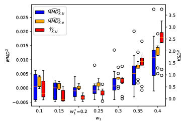
(a) small-sample case

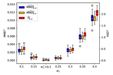
(b) large-sample case

Figure 3: Boxplots of the objective values for Gaussian returns ($\mathbb{P}_{R}$) and Gaussian kernel ($K$). Plotted: $w_{1}\mapsto\widehat{\operatorname{MMD}}_{K,U}^{2}\left(\mathbb{P}_{\mathbf{w},N},\mathbb{P}_{T,M}\right),\widehat{\operatorname{MMD}}_{K,e}^{2}\left(\mathbb{P}_{\mathbf{w},N},\mathbb{P}_{T}\right),\hat{\text{T}}^{2}_{K,U}\left(\mathbb{P}_{\mathbf{w},N},\mathbb{P}_{T}\right)$, with portfolio weight $\mathbf{w}=[w_{1};1-w_{1}]$. The optimal portfolio weight is $\mathbf{w}^{*}=[w_{1}^{*};1-w_{1}^{*}]$ with $w_{1}^{*}=0.2$. Left: $N=100$ samples. Right: $N=5\times 10^{3}$ samples.

We illustrate the evolution of the various objectives as a function of $\mathbf{w}=[w_{1};1-w_{1}]$ by varying the value of $w_{1}$ in the set $\{0.1,0.15,0.2,\dots,0.4\}$. We consider two different situations: one is the large-sample case ($N=M=5000$), the other is the small-sample case ($N=M=100$). We evaluate the objectives on samples $\{\mathbf{r}_{i}\}_{i\in[N]}\stackrel{{\scriptstyle\text{i.i.d.}}}{{\sim}}{\cal{N}}\left(\bm{m}_{R},\Sigma_{R}\right)$ and $\{t_{i}\}_{i\in[M]}\stackrel{{\scriptstyle\text{i.i.d.}}}{{\sim}}{\cal{N}}\left(m,\sigma^{2}\right)$ where $m$ and $\sigma^{2}$ are defined in (29). The kernel bandwidth $c$ was taken to be equal to the standard deviation of $\{\mathbf{w}^{\top}\mathbf{r}_{i}\}_{i\in[N]}$ for each $\mathbf{w}=[w_{1};1-w_{1}]$. In order to investigate the robustness of the estimators, we report the median values, quartiles and extreme values of the estimators as a function of the weight $w_{1}$ using $15$ repetitions. The corresponding summary statistics are available in Fig. 3. As the figure shows the estimated MMD and Stein objectives follow a U-shape as a function of $w_{1}$ and take their minimum at $w_{1}^{*}=0.2$. Notice that the scale on the y-axis is different for the MMD estimators (l.h.s.) and for the Stein estimator (r.h.s.); the latter increases more rapidly as we move away from $w_{1}^{*}=0.2$. In accordance with Theorem 3.4 the semi-explicit MMD estimator shows improved concentration properties, and this behavior is particularly emphasized in the small-sample regime.

Gaussian returns, exponential kernel: In this experiment, we follow the same assumption of Gaussian returns, but we consider the unbounded exponential kernel $K(x,y)=e^{bxy}$ with $b>0$. The two-sample MMD estimator is calculated via (17). The semi-explicit MMD objective (18) is obtained by using the explicit mean embedding $\mu_{K}(\mathbb{P}_{T})(x)$ given in Lemma 3.1 and by the relation

$$\mathbb{E}_{t\sim\mathbb{P}_{T}}\mu_{K}(\mathbb{P}_{T})(t)=\frac{e^{\frac{bm^{2}}{1-b\sigma^{2}}}}{\sqrt{1-(b\sigma^{2})^{2}}},$$

which is derived in (35). We chose $b=\frac{1}{2\hat{\sigma}^{2}}$ with $\hat{\sigma}$ being the standard deviation of $\{\mathbf{w}^{\top}\mathbf{r}_{i}\}_{i\in[N]}$ for each $\mathbf{w}=[w_{1};1-w_{1}]$. The evaluation is made on $N=M=10^{4}$ samples, with $50$ repetitions for each $w_{1}$.

Figure 4: Boxplots of the objective values for Gaussian return ($\mathbb{P}_{R}$) and exponential kernel ($K$). Plotted: $w_{1}\mapsto\widehat{\operatorname{MMD}}_{K,U}^{2}\left(\mathbb{P}_{\mathbf{w},N},\mathbb{P}_{T,M}\right)$ and $w_{1}\mapsto\widehat{\operatorname{MMD}}_{K,e}^{2}\left(\mathbb{P}_{\mathbf{w},N},\mathbb{P}_{T}\right)$, with portfolio weight $\mathbf{w}=[w_{1};1-w_{1}]$. The optimal portfolio weight is $\mathbf{w}^{*}=[w_{1}^{*};1-w_{1}^{*}]$ with $w_{1}^{*}=0.2$. Right: left plot zoomed in.

The resulting median values, quartiles and extreme values of the estimators are summarized in Fig. 4. The figure shows that (i) again the semi-explicit MMD estimator has better concentration properties than the two-sample MMD one, (ii) the U-shape of the objective values is less pronounced with the exponential kernel, (iii) by zooming in to the estimated objectives curves they still take their minimum around the optimal weight $w_{1}^{*}=0.2$.

beta returns, Laplacian kernel: In this experiment the return variable $R\in\mathbb{R}^{2}$ has components with beta distribution, and the kernel is the Laplacian $K(x,y)=e^{\lambda\lvert x-y\rvert}$ with $\lambda>0$. The parameters of the beta target distribution are set by moment matching (recalled in Table 12) applied to (29).

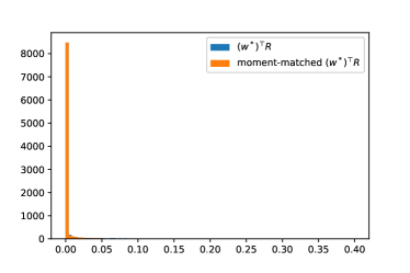
Figure 5: Comparison of the histogram of the portfolio returns $(\mathbf{w}^{*})^{\top}R$ (with $R$ having beta components) and one-dimensional beta target distribution with the same mean and variance on $10^{4}$ samples. Right: left plot zoomed in.

In the $\widehat{\operatorname{MMD}}_{K,U}^{2}\left(\mathbb{P}_{\mathbf{w},N},\mathbb{P}_{T,M}\right)$ and semi-explicit $\widehat{\operatorname{MMD}}_{K,e}^{2}\left(\mathbb{P}_{\mathbf{w},N},\mathbb{P}_{T}\right)$ estimators [(15) and (18)], we discard the 2nd terms which are independent of $\mathbf{w}$; hence the objective values can easily take negative values. We chose $\lambda=\frac{1}{2\hat{\sigma}}$ with $\hat{\sigma}$ being the standard deviation of $\{\mathbf{w}^{\top}\mathbf{r}_{i}\}_{i\in[N]}$ for each $\mathbf{w}=[w_{1};1-w_{1}]$. The evaluation was carried out using $N=M=10^{4}$ samples. The boxplots of the resulting objective values as a function of the portfolio weight $w_{1}$ derived from $15$ repetitions are summarized in Fig. 6. As it can be seen, the analytical knowledge of the mean embedding is again beneficial: the objective values obtained using the semi-explicit MMD estimator follow a more emphasized U-shape behavior.

Figure 6: Boxplots of the objective values for beta return ($\mathbb{P}_{R}$) and Laplacian kernel ($K$). Plotted: $w_{1}\mapsto\widehat{\operatorname{MMD}}_{K,U}^{2}\left(\mathbb{P}_{\mathbf{w},N},\mathbb{P}_{T,M}\right)$ and $w_{1}\mapsto\widehat{\operatorname{MMD}}_{K,e}^{2}\left(\mathbb{P}_{\mathbf{w},N},\mathbb{P}_{T}\right)$, with portfolio weight $\mathbf{w}=[w_{1};1-w_{1}]$. The optimal portfolio weight is $\mathbf{w}^{*}=[w_{1}^{*};1-w_{1}^{*}]$ with $w_{1}^{*}=0.2$.

These experiments demonstrate the efficiency of the proposed technique. Our theoretical and numerical results show that the semi-explicit MMD has improved concentration property compared to the two-sample MMD estimator. The Gaussian kernel leads to more pronounced U-shape of the objectives than the unbounded kernel, and suggests easier optimization. The unbounded support of Gaussian targets is better motivated in finance compared to the bounded one of the beta target. Hence we keep the Gaussian target for our subsequent numerical studies. The next subsection is dedicated to the exploration of the efficiency of our technique in the misspecified setting.

4.2 Misspecified setting

In this section, we study the impact of misspecification, in other words when $D(P_{\mathbf{w}^{*}},P_{T})\neq 0$. In particular, we investigate the case when $d=2$, the target distribution is Gaussian, and the first coordinate $R_{1}$ of the returns $R=[R_{1};R_{2}]\in\mathbb{R}^{2}$ is generalized normal, its second coordinate $R_{2}$ is normal. We assume that there exists an initial portfolio $\mathbf{w}_{0}=[x;1-x]\in\mathscr{W}$. The target distribution $\mathbb{P}_{T}$ is chosen to be equal to the distribution of $(\mathbf{w}_{0})^{\top}R\in\mathbb{R}$ with $\gamma=2$. Our goal is to study the impact on the estimated optimal portfolio

$$\mathbf{w}^{*} :=[x^{*};1-x^{*}]:=\operatorname*{arg\,min}_{\mathbf{w}\in\mathscr{W}}D\left(\mathbb{P}_{\mathbf{w},N},\mathbb{P}_{T}\right)$$

as a function of the heavy-tailness parameter $\gamma<2$ when the underlying $\mathbf{w}$ is changed slightly, and to explore if $x^{*}$ turns into smaller than $x$ (less weight is allocated on the heavy-tailed component) or if $x^{*}$ becomes higher than $x$ (more weight is allocated on the heavy-tailed component). Denoting by $\varepsilon>0$ the measure of local perturbation, and by $\mathbf{w}_{0}^{-}=[(x-\varepsilon);1-(x-\varepsilon)]$ and $\mathbf{w}_{0}^{+}=[x+\varepsilon;1-(x+\varepsilon)]$ the corresponding portfolio weights, let

$$\mathbf{w}^{\min} :=[x^{\min};1-x^{\min}]:=\operatorname*{arg\,min}_{\mathbf{w}\in\left\{\mathbf{w}_{0}^{-},\mathbf{w}_{0},\mathbf{w}_{0}^{+}\right\}}D\left(\mathbb{P}_{\mathbf{w},N},\mathbb{P}_{T}\right)$$

be the weight with the lowest divergence among these 3 allocations. The sign of the optimal allocation variation is $\operatorname{sign}{\Delta x}=\operatorname{sign}{x^{*}-x}=\operatorname{sign}{x^{\min}-x}$. In our experiments, the heavy-tailness parameter was chosen to be $\gamma=1$ (which gives rise to the Laplace distribution), we used the semi-explicit MMD as divergence estimator with sample size $N=10^{4}$, and we set $\varepsilon=0.1$. The mean $\bm{m}_{R}=\begin{bmatrix}m_{1}\\ m_{2}\end{bmatrix}$ and the covariance matrix $\bm{\Sigma}_{R}=\begin{bmatrix}\sigma_{1}^{2}&0\\ 0&\sigma_{2}^{2}\end{bmatrix}$ of $R$ was generated randomly from $m_{i}\sim\mathcal{U}[0.01,0.05]$ and $\sigma^{2}_{i}\sim\mathcal{U}[0.01,0.06]$. The initial portfolio weight $\mathbf{w}=[x;1-x]$ was varied by changing $x\in\{0,0.1,0.2,\ldots,0.9,1\}$. Let $\left[\Delta m,\Delta\sigma^{2}\right]:=\left[m_{2}-m_{1};\sigma^{2}_{2}-\sigma^{2}_{1}\right]$ and $\Delta\gamma=1-2=-1$.

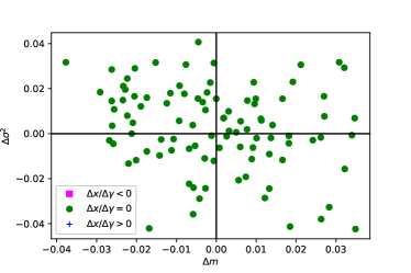
(a) $x=0.1$

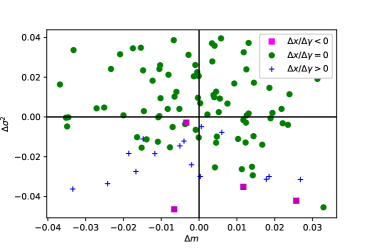
(b) $x=0.4$

(c) $x=0.5$

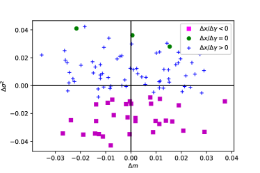
(d) $x=0.7$

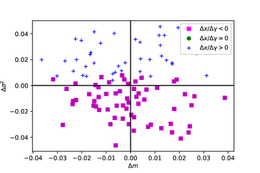
(e) $x=0.8$

(f) $x=1.$

Figure 7: Plots of randomly simulated $(\Delta\mu,\Delta\sigma)$ pairs colored by their associated sign of $\frac{\Delta x}{\Delta\gamma}$. Magenta: $\frac{\Delta x}{\Delta\gamma}<0$. Blue: $\frac{\Delta x}{\Delta\gamma}>0$. Green: $\frac{\Delta x}{\Delta\gamma}=0$. The subfigures correspond to different $x$ weights.

Fig. 7 illustrates $10^{4}$ pairs of $(\Delta m,\Delta\sigma^{2})$ colored by the associated sign of $\frac{\Delta x}{\Delta\gamma}$; each subfigure corresponds to a specific choice of weight $x$. Positive sign of $\frac{\Delta x}{\Delta\gamma}$ means that the optimal allocation turns to be less concentrated on the heavy-tailed component ($\Delta x<0$) when the initial return distribution has one component with heavier tails than the target ($\Delta\gamma<0$). Conversely, negative sign of $\frac{\Delta x}{\Delta\gamma}$ shows that the new allocation becomes more concentrated on the heavy-tailed component. As it can be seen in the figure, there is no systematic decrease of the allocation associated to the heavy-tailed component, rather there is an interplay between the variance variation $\Delta\sigma^{2}$ and the initial value $x$, without $\Delta m$ affecting the results. For low values of $x$ ($x\leq 0.4$) heavy-tailness has limited impact, for ”balanced” initial portfolios ($0.5\leq x\leq 0.7$) and $\Delta\sigma^{2}>0$ we retrieve the expected lower weight on heavy-tailed component, for larger $x$ and negative $\Delta\sigma^{2}$ the new optimal portfolio becomes more concentrated on the heavy-tailed component. These experiment show that larger variance or concentration lead to more weight on the heavy-tailed component. One can explain this phenomena using the fact that heavy-tailed distributions with high variance have more extreme values, which affect the divergence matching.

5 Experiments on financial time series

In this section, we demonstrate the efficiency of the investigated target distribution technique for portfolio optimization. The considered datasets, rebalancing, performance measures and target distributions are summarized in Section 5.1, followed by the numerical studies in Section 5.2.

5.1 Datasets, rebalancing, performance measures, target distributions

This section summarizes the neccessary ingredients of the numerical experiments.

Datasets: We selected 2 representative portfolio datasets (see Table 7) from the Kenneth French’s library [13] (also used in the recent extensive numerical study carried out by [33]). The 6BTM benchmark is based on the size, book-to-market and operating profitability performance indicators. The dataset components are built as the linear combination of stock returns from the NYSE market equity sorted by two main indicators. For example, the first component of 6BTM corresponds to a linear combination of small size (or market equity) and high book-to-market ratio (or low growth), small meaning belonging to the the first half (size criteria) and $70-100\%$ percentile (book-to-market ratio criteria) bucket; see Fig. 8 for an illustration of the price evolution of $2$ components of this benchmark. For this dataset the portfolio size is $d=6$. Our second portfolio dataset is referred to as 10Ind, and it corresponds to the linear combination of stock returns by sector of activity, with portfolio size $d=10$. The variance of the components of the two datasets is illustrated in Fig. 9. As the figure shows the variance is more balanced in the 6BTM than on the 10Ind dataset; in case of the latter the higher variance components correspond to Energy, HighTech and Durables. According to our misspecification study (Section 4.2), the target distribution technique is expected to perform better on the 6BTM dataset. The average excess kurtosis is $15.1$ for the 6BTM and $14.5$ for the 10Ind benchmark. The average skewnesses are negative, equal to $-0.58$ and $-0.37$, respectively. These statistics corresponds to a heavy-tailed and negatively-skewed setting. In Fig. 10, we display the evolution of the returns of the 6BTM and 10Ind portfolios. One can notice periods of high and low volatility; the periods of high volatility occur at the same time points in the two datasets. To study the dependence of the target distribution technique on market conditions (low-volatility and high-volatility periods, corresponding to normal economic conditions and potential crisis periods), the datasets were split in two sub-samples. The considered quantitative criteria to distinguish these two regimes consists in comparing the semi-annual average variance to the average variance over the $41$ years of data, as displayed in Fig. 10(c). When the annual variance is larger than $1.5$ times the long-term average variance, we say that we are in a high-volatility/crisis period. There are $7$ buckets out of $71$ (specified by the rolling window approach detailed below) that this criteria considers to be highly volatile.

Dataset	Abbreviation	$d$
6 Fama-French portfolios of firms sorted by size and book-to-market	6BTM	6
10 industry portfolios representing the US stock market	10Ind	10

Table 7: Financial datasets used in our empirical study. They are composed of daily value-weighted arithmetic returns from January 1980 to December 2020. Total number of samples: $N=10318$.

Figure 8: Price evolution associated to the first and last component of the 6BTM datasets. The prices ($P_{t}$) are calculated from returns ($r_{t}$) data as $P_{t}=P_{t-1}(1+r_{t})$ where we fixed $P_{0}=1$.

(a) 6BTM

(b) 10Ind

Figure 9: Variance of the component returns of the 6BTM (a) and the 10Ind dataset (b).

(a) 6BTM

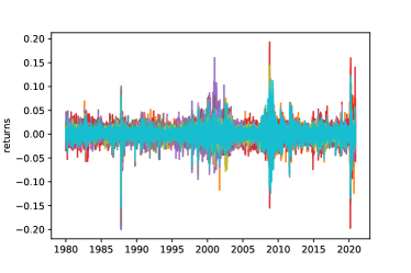
(b) 10Ind

(c) Semi-annual variance - 6BTM

Figure 10: Superposition of the component returns of the 6BTM (a) and the 10Ind dataset (b). In (c) the semi-annual variance of the 6BTM returns is shown. There are volatility clusters in 1988, 2000, 2007 and 2020 (due to financial crisis/inflation/Covid-19) in both datasets.

Rebalancing, performance measures: For a fair numerical comparison we use the same rebalancing methodology as [33] in his recent extensive study. An estimation window of $5$ years and a rolling window (interval on which the output statistics are computed) of six months were considered. On our $41$ years of data, it makes $71$ buckets on which the out-of-sample performance of the portfolio is evaluated in terms of kurtosis and skewness. Our benchmark portfolio allocation strategies with their abbreviations are listed in Table 8. They correspond to the best-performing traditional and minimum divergence portfolio of the recent report [33, Section 5.7.3].

Portfolio	Abbreviation	Reference
sample minimum variance portfolio	MV	[27]
Bayes-Stein maximum Sharpe ratio portfolio	MSR	[29]
minimum Kullback-Leibler portfolio with Gaussian target	KL	[33] (4)

Table 8: State-of-the-art portfolios [33].

Target distributions: In practice, financial returns exhibit positive excess kurtosis and negative skewness. These properties are referred to as stylized facts [9]. Hence the returns cannot be considered Gaussian or elliptical (and hence described solely by their mean and variance). Considering standard concave and increasing utility maximisation framework [40] it can be showed that investors prefer higher skewness and lower kurtosis. Targeting lighter-tailed distribution (via for example generalized normal distribution) or more positively skewed distributions (for instance with skew Gaussian target) should have a favorable impact regarding the out-of-sample moments of the minimum-divergence portfolio compared to traditional mean-variance portfolios. In our numerical studies, we are going to focus on three families of target distributions: (i) the Gaussian distribution for which explicit mean embedding is available for various kernel choices (see Table 5), (ii) the generalized normal distribution with parameter $\gamma$ allowing to target negative excess kurtosis when chosen $\gamma>2$, (iii) the skew Gaussian distribution with parameter $c$ allowing to target positive skewness with $c>0$. In the latter two cases, we chose light-tailed generalized normal ($\gamma=4$), and positively skewed skew Gaussian distribution ($s=1$, in this case the excess kurtosis is $0.0617$ by Table 12, hence very close to $0$) as targets. We fixed the target mean and standard deviation as given by the maximum Sharpe ratio portfolio (in sample mean and standard-deviation associated to the maximum Sharpe ratio allocation). We summarize in Table 9 our choices of target distributions and divergences, noting that the linear-time FSSD provides a faster alternative to the quadratic-time KSD divergence.

Divergence ($D$)	Target distribution ($\mathbb{Q}$)
semi-explicit MMD	Gaussian
MMD with low-rank approximation	Gaussian, generalized normal, skew Gaussian
KSD	Gaussian
FSSD	Gaussian, generalized normal, skew Gaussian
WAD with $p=1$	Gaussian, generalized normal, skew Gaussian
WAD with $p=2$	Gaussian, generalized normal, skew Gaussian
KL	Gaussian

Table 9: Tested divergence - target distribution pairs.

5.2 Numerical studies

In this section, the out-of-sample kurtosis and skewness of our divergence-based portfolios versus the traditional minimum variance and maximum Sharpe ratio portfolios are compared, across different datasets and economic conditions. Kurtosis is investigated in Section 5.2.1, we focus on skewness in Section 5.2.2; in these sections the low and high-volatity regimes are studied separately. Section 5.2.3 provides an overall assessment with low and high-volatility periods merged.

In our experiments, we made use of the KGOF and ITE toolbox packages [55, 55] when computing the FSSD and the two-samples MMD divergence measures.

5.2.1 Kurtosis impact

In this section, the impact on the portfolio kurtosis is investigated. We report the out-of-sample (OOS) excess kurtosis values for the different divergence objectives considered, and compare them to the traditional minimum variance portfolio (MV) and the maximum Sharpe ratio (MSR) portfolio. Lower kurtosis is an indication of less heavy tails, and this is what is usually advantageous from financial point of view, in other words more negative (or at least closer to zero) excess kurtosis corresponds to better performing portfolio.

Normal economic conditions: The OOS kurtosis values with generalized normal and skew Gaussian targets are summarized in Fig. 12. For both datasets, the MMD-based divergences give lower median kurtosis than the WAD-based portfolios and the traditional portfolios, and the lower quartile for most divergence based portfolios is lower than that of the traditional portfolios.

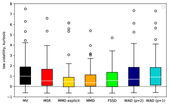
(a) skew Gaussian, 6BTM

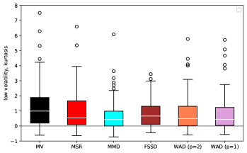
(b) generalized normal, 6BTM

(c) skew Gaussian, 10Ind

(d) generalized normal, 10Ind

Figure 11: OOS kurtosis values in the low-volatility regime. Left: baselines (MV, MSR). Right: proposed minimum divergence portfolios with skew Gaussian (1st column) and generalized normal (2nd column) target. 1st row: 6BTM dataset. 2nd row: 10Ind benchmark.

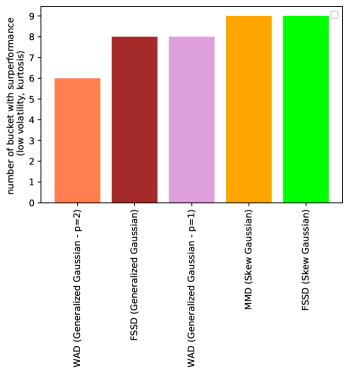
(a) 6BTM

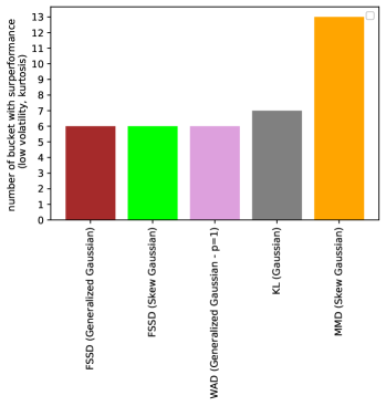
(b) 10Ind

Figure 12: The five top objective-target pairs in kurtosis sense. Regime: low-volatility. Ordering: from worst (left) to best (right). (a): 6BTM dataset. (b): 10Ind benchmark.

In Fig. 12, we provide the barplots of the number of buckets (time periods) on which a given objective-target pair achieved the lowest kurtosis across all the objectives; they are sorted by increasing efficiency and we show the $5$ winners. On the 6BTM dataset, the $5$ winners correspond to light-tailed target distributions (skew or generalized normal) with similar performance. On the 10Ind benchmark, MMD with skew Gaussian target performs the best, followed by the minimum KL approach using Gaussian target (which has heavier tails than the skew Gaussian distribution). This (i) means that light-tailed targets are not predominant here, and the reason for this can be that the 10Ind dataset is a more heterogeneous than 6BTM as it can be seen from the variance barplots in Fig. 9.

High-volatility conditions: In high-volatility scenarios on both datasets the results are more diverse, see Fig. 13. For the 6BTM benchmark, MMD with skew Gaussian target and FSSD with generalized normal target lead to relatively small kurtosis. On the 10Ind dataset, WAD ($p=1$) with generalized normal target also seems to perform well.

Considering the Gaussian target (which gives rise to analytical divergence computations and targets with $0$ kurtosis which is lower than the average $~{}14-15$ kurtosis value of the datasets), the OOS kurtosis values obtained for various divergences are summarized in Fig. 14. In the high-volatility regime Fig. 14(b), the semi-explicit MMD and the KSD portfolios give more concentrated kurtosis values compared to the low-rank MMD approximation; this phenomenon can be explained due to the lack of sampling needed from the target distribution. These effects are less pronounced in the low-volatility regime, see Fig. 14(a).

(a) skew Gaussian, 6BTM

(b) generalized normal, 6BTM

(c) skew Gaussian, 10Ind

(d) generalized normal, 10Ind

Figure 13: OOS kurtosis boxplots in the high-volatility regime. Left: baselines (MV, MSR). Right: proposed minimum divergence portfolios with skew Gaussian (1st column) and generalized normal (2nd column) target. 1st row: 6BTM benchmark. 2nd row: 10Ind dataset.

(a) low volatility

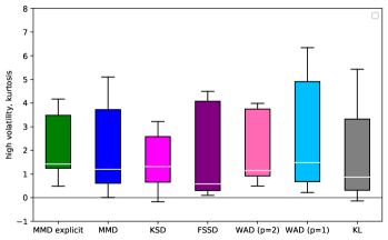
(b) high volatility

Figure 14: OOS kurtosis values for minimum divergence portfolios with the Gaussian target. Period: low-volatility (a), high-volatility (b). Dataset: 10Ind.

5.2.2 Skewness impact

In this section, the impact on the portfolio skewness is investigated. We report the OOS excess skewness values for the different divergence objectives considered, and compare them to the traditional minimum variance portfolio (MV) and the maximum Sharpe ratio (MSR) portfolio. Higher skewness is an indication of less negatively skewed distribution, and this is what is usually beneficial from financial perspective, in other words more positive (or at least closer to zero) excess skewness is interpreted as better performing portfolio.

Normal economic conditions: The OOS skewness values with generalized normal and skew Gaussian targets are summarized in Fig. 16. For both datasets, the skew Gaussian target with either MMD or FSSD divergence give the highest median skewness and the lower quartile for most divergence based portfolios is higher than that of the traditional portfolios. The latter behavior is particularly apparent on the 6BTM benchmark with the generalized normal target.

In Fig. 16, we provide the barplots of the number of buckets on which a given objective-target pair achieved the highest skewness across all the objectives; we show the $5$ winners. On both datasets, the top performers correspond to light-tailed target distributions (skew or generalized normal). We also see that the WAD objective with $p=1$ is performing well on the 6BTM dataset.

High-volatility conditions: In high-volatility scenarios on both datasets the results are more diverse, see Fig. 17. The skewness of traditional portfolios is not necessarily negative. As for the kurtosis, the target-distribution portfolio approach seems to have more impact in normal economic conditions. For the 6BTM benchmark, MMD-based objectives give a larger median skewness than the traditional portfolios. On the 10Ind dataset, only FSSD with generalized normal target succeeds in beating the traditional portfolios, but with quite a large margin in terms of the upper quartile.

(a) skew Gaussian, 6BTM

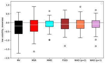
(b) generalized normal, 6BTM

(c) skew Gaussian, 10Ind

(d) generalized normal, 10Ind

Figure 15: OOS skewness values in the low-volatility regime. Left: baselines (MV, MSR). Right: proposed minimum divergence portfolios with skew Gaussian (1st column) and generalized normal (2nd column) target. 1st row: 6BTM dataset. 2nd row: 10Ind benchmark.

(a) 6BTM

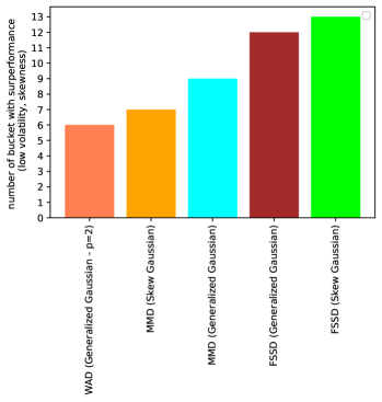
(b) 10Ind

Figure 16: The five top objective-target pairs in skewnesss sense. Regime: low-volatility. Ordering: from worst (left) to best (right). (a): 6BTM dataset. (b): 10Ind benchmark.

(a) skew Gaussian, 6BTM

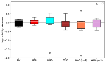
(b) generalized normal, 6BTM

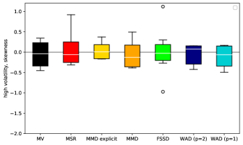
(c) skew Gaussian, 10Ind

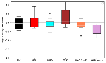
(d) generalized normal, 10Ind

Figure 17: OOS skewness boxplots in the high-volatility regime. Left: baselines (MV, MSR). Right: proposed minimum divergence portfolios with skew Gaussian (1st column) and generalized normal (2nd column) target. 1st row: 6BTM benchmark. 2nd row: 10Ind dataset.

5.2.3 Merged results

In this section, we comment the barplots of Fig. 18 corresponding to the number of buckets on which a given objective-target pair achieved the highest kurtosis or skewness across all the objectives, across all the buckets (with low and high volatility scenarios merged). For both benchmarks, the clear winners are

• MMD with skew Gaussian target (orange, present in all $4$ subfigures),

• FSSD with generalized normal target (dark red, present in $3$ subfigures, 1st/2nd place in $2$ of them),

• Wasserstein distance ($p=1$) with generalized normal target (mauve, present in $3$ subfigures, 1st/2nd position in $2$ cases),

• Kullback-Leibler divergence with Gaussian target (grey), especially on the 10Ind dataset.

The good performance of the WAD divergence (with $p=1$) might be due to the outlier-robust character of $L_{1}$-based objective functions. Overall, the best performing portfolios are in majority associated to light-tail distribution targets, except for the KL-Gaussian which performs well on the 10Ind dataset. The final barplots in Fig. 18 show more homogeneity on the 6BTM datasets (in terms of kurtosis), many objective functions are performing similarly.

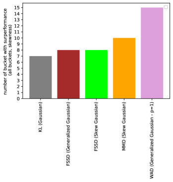
(a) skewness, 6BTM

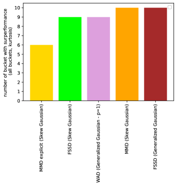
(b) kurtosis, 6BTM

(c) skewness, 10Ind

(d) kurtosis, 10Ind

Figure 18: The five top objective-target pairs. Regime: low and high-volatility merged. Ordering: from worst to best in skewness sense (1st column) and kurtosis sense (2nd column). 1st row: 6BTM benchmark. 2nd row: 10Ind dataset.

6 Conclusion

In this paper, we focused on kernel-based divergence measures and their application in financial portfolio optimization using the target distribution framework. We showed that prior knowledge available on target distribution leads to analytical forms for the mean embedding (Lemma 3.1 and Lemma 3.2) and improved MMD concentration properties for bounded kernels (Theorem 3.4). Motivated by recent financial studies relying on unbounded kernels [5], using the Burkholder inequality we proved that the $1/\sqrt{N}$ rate (with $N$ denoting the sample size) of MMD estimators can be extended to unbounded kernels (Theorem 3.5); we illustrated the idea for the exponential kernel. We showed matching minimax lower bounds (Theorem 3.6) under slightly more restrictive conditions.

We illustrated the effectiveness of the resulting semi-explicit MMD estimator over the classical two-sample MMD estimator not relying on the knowledge of mean embedding on simulated examples. We demonstrated the proposed kernel-based divergence framework in real-world portfolio optimization problems. According to our numerical experiences, the proposed technique

• performs favorably compared to classical portfolio optimization scheme on balanced portfolios in normal economic conditions,

• MMD and KSD with light-tailed targets often improves the out-of-sample skewness and kurtosis of the portfolio.

Our preliminary results on alternative statistics show that the information theoretical technique can have slightly higher turnover than traditional schemes, which makes it an ideal candidate as a regularizer added to the global portfolio optimization objective.

Appendix A Proofs

This section contains the proofs of theoretical results. In Section A.1 we give the proofs of the two analytical mean embedding results (Lemma 3.1 and Lemma 3.2), accompanied by two additional lemmas used in Section 4.1 and in the proof of Theorem 3.6, respectively. Section A.2 is dedicated to the proof of our concentration results (Theorem 3.4, Theorem 3.5, Theorem 3.6).

A.1 Proofs of auxiliary statements

In this section we prove Lemma 3.1 and Lemma 3.2. These proofs are accompanied by two additional auxiliary statements (Lemma A.3 and Lemma A.5). Lemma A.3 is on the Stein kernel for the Gaussian distribution - Gaussian kernel, Lemma A.5 is about MMD for the Gaussian distribution and the exponential kernel. The former is used in the KSD computation in Section 4.1; the latter is applied in the reasoning of Theorem 3.6.

Proof A.1.

(Lemma 3.1; mean embedding: Gaussian target - Gaussian-exponentiated kernel) Our target quantity is

$$\mu_{K}(\mathbb{Q})(x) =\int_{\mathbb{R}}\frac{1}{\sqrt{2\pi\sigma^{2}}}{e}^{-{\frac{\left(y-m\right)^{2}}{2\sigma^{2}}}}e^{-a(x-y)^{2}+bxy}\mathrm{d}y.$$

Completing the square, one gets

$$\frac{\left(y-m\right)^{2}}{2\sigma^{2}}+a(x-y)^{2}-bxy=\frac{\left(y-m\right)^{2}+2\sigma^{2}a(x-y)^{2}-2\sigma^{2}bxy}{2\sigma^{2}}=$$

$$=\frac{\left(1+2a\sigma^{2}\right)y^{2}-2\left(m+2a\sigma^{2}x+b\sigma^{2}x\right)y+2a\sigma^{2}x^{2}+m^{2}}{2\sigma^{2}}$$

$$=\underbrace{\frac{(1+2a\sigma^{2})}{2\sigma^{2}}}_{=:\frac{1}{2{\sigma^{*}}^{2}}}\bigg{(}y^{2}-2\underbrace{\frac{m+2a\sigma^{2}x+b\sigma^{2}x}{1+2a\sigma^{2}}}_{=:m^{*}}y\bigg{)}+\frac{2a\sigma^{2}x^{2}+m^{2}}{2\sigma^{2}}$$

$$=\frac{1}{2{\sigma^{*}}^{2}}\left[\left(y-m^{*}\right)^{2}-{m^{*}}^{2}\right]+\frac{2a\sigma^{2}x^{2}+m^{2}}{2\sigma^{2}}$$

$$=\frac{1}{2{\sigma^{*}}^{2}}\left(y-m^{*}\right)^{2}\underbrace{-\frac{(m+2a\sigma^{2}x+b\sigma^{2}x)^{2}}{2\sigma^{2}(1+2a\sigma^{2})}+\frac{2a\sigma^{2}x^{2}+m^{2}}{2\sigma^{2}}}_{=:-c^{*}}.$$

Bringing the two terms in $c^{*}$ to common denominator, after simplification on arrives at

$$c^{*} =\frac{\left(m+2a\sigma^{2}x+b\sigma^{2}x\right)^{2}-\left(2a\sigma^{2}x^{2}+m^{2}\right)\left(1+2a\sigma^{2}\right)}{2\sigma^{2}\left(1+2a\sigma^{2}\right)}$$

$$=\frac{4a\sigma^{2}mx-2a\sigma^{2}(m^{2}+x^{2})+b\sigma^{2}x\left(b\sigma^{2}x+4a\sigma^{2}x+2m\right)}{2\sigma^{2}(1+2a\sigma^{2})}$$

$$=\frac{-2a\sigma^{2}(m-x)^{2}+b\sigma^{2}x\left(b\sigma^{2}x+4a\sigma^{2}x+2m\right)}{2\sigma^{2}\left(1+2a\sigma^{2}\right)}$$

$$=-\frac{a(x-m)^{2}}{1+2a\sigma^{2}}+\frac{2bmx+b\sigma^{2}(b+4a)x^{2}}{2(1+2a\sigma^{2})}.$$

This means that our target quantity can be rewritten as

$$\mu_{K}(\mathbb{Q})(x) =\int_{\mathbb{R}}\frac{1}{\sqrt{2\pi\sigma^{2}}}e^{-\frac{1}{2{\sigma^{*}}^{2}}\left(y-m^{*}\right)^{2}+c^{*}}\mathrm{d}y=\frac{\sigma^{*}}{\sigma}e^{c^{*}}\underbrace{\int_{\mathbb{R}}\frac{1}{\sqrt{2\pi(\sigma^{*})^{2}}}e^{-\frac{1}{2{\sigma^{*}}^{2}}\left(y-m^{*}\right)^{2}}\mathrm{d}y}_{=1}$$

$$=\frac{e^{-\frac{a(x-m)^{2}}{1+2a\sigma^{2}}+\frac{2bmx+b(b+4a)\sigma^{2}x^{2}}{2(1+2a\sigma^{2})}}}{\sqrt{1+2a\sigma^{2}}}.$$

Proof A.2.

(Lemma 3.2; mean embedding: beta target - Matérn kernel) Our target quantity is

$$\mu_{K}(\mathbb{Q})(x)=$$

$$=\frac{\sigma_{0}^{2}}{B(\alpha,\beta)}\int_{0}^{1}e^{-{\frac{{\sqrt{2p+1}}|x-y|}{\sigma}}}{\frac{p!}{(2p)!}}\sum_{i=0}^{p}{\frac{(p+i)!}{i!(p-i)!}}\left({\frac{2{\sqrt{2p+1}}|x-y|}{\sigma}}\right)^{p-i}y^{\alpha-1}(1-y)^{\beta-1}\mathbb{I}_{y\in[0,1]}\mathrm{d}y$$

$$\stackrel{{\scriptstyle(*)}}{{=}}\frac{\sigma_{0}^{2}}{B(\alpha,\beta)}\frac{p!}{(2p)!}\sum_{i=0}^{p}{\frac{(p+i)!}{i!(p-i)!}}\left({\frac{2{\sqrt{2p+1}}}{\sigma}}\right)^{p-i}\bigg{[}\int_{0}^{(0\vee x)\wedge 1}(x-y)^{p-i}y^{\alpha-1}(1-y)^{\beta-1}e^{-{\frac{{\sqrt{2p+1}}(x-y)}{\sigma}}}\mathrm{d}y$$

$$\hskip 227.62204pt+\int_{(0\vee x)\wedge 1}^{1}(y-x)^{p-i}y^{\alpha-1}(1-y)^{\beta-1}e^{-{\frac{{\sqrt{2p+1}}(y-x)}{\sigma}}}\mathrm{d}y\bigg{]},$$

where in $(*)$ we applied the decomposition trick: for $f:\mathbb{R}\rightarrow\mathbb{R}$ and $x\in\mathbb{R}$,

$$\int_{0}^{1}f(|x-y|)\mathrm{d}y=\int_{0}^{(0\vee x)\wedge 1}f(x-y)\mathrm{d}y+\int_{(0\vee x)\wedge 1}^{1}f(y-x)\mathrm{d}y.$$

Using the binomial formula on $(x-y)^{p-i}=\sum_{k=0}^{p-i}{p-i\choose k}x^{k}(-y)^{p-i-k}$ and on $(y-x)^{p-i}$, one can rewrite the two integrals as

$$\int_{0}^{(0\vee x)\wedge 1}(x-y)^{p-i}y^{\alpha-1}(1-y)^{\beta-1}e^{-{\frac{{\sqrt{2p+1}}(x-y)}{\sigma}}}\mathrm{d}y=$$

$$=\sum_{k=0}^{p-i}{p-i\choose k}(-1)^{p-i-k}x^{k}\int_{0}^{(0\vee x)\wedge 1}y^{p-i-k}y^{\alpha-1}(1-y)^{\beta-1}e^{-{\frac{{\sqrt{2p+1}}(x-y)}{\sigma}}}\mathrm{d}y$$

$$=\sum_{k=0}^{p-i}{p-i\choose k}(-1)^{p-i-k}x^{k}e^{-{\frac{{\sqrt{2p+1}}x}{\sigma}}}\underbrace{\int_{0}^{(0\vee x)\wedge 1}y^{p-i-k+\alpha-1}(1-y)^{\beta-1}e^{{\frac{{\sqrt{2p+1}}y}{\sigma}}}\mathrm{d}y}_{E_{1}^{\frac{{\sqrt{2p+1}}}{\sigma}}\left((0\vee x)\wedge 1,p-i-k+\alpha-1,\beta-1\right)},$$

and

$$\int_{(0\vee x)\wedge 1}^{1}(y-x)^{p-i}y^{\alpha-1}(1-y)^{\beta-1}e^{-{\frac{{\sqrt{2p+1}}(y-x)}{\sigma}}}\mathrm{d}y=$$

$$=\sum_{k=0}^{p-i}{p-i\choose k}(-x)^{k}\int_{0}^{(0\vee x)\wedge 1}y^{p-i-k}y^{\alpha-1}(1-y)^{\beta-1}e^{-{\frac{{\sqrt{2p+1}}(y-x)}{\sigma}}}\mathrm{d}y$$

$$=\sum_{k=0}^{p-i}{p-i\choose k}(-x)^{k}e^{{\frac{{\sqrt{2p+1}}x}{\sigma}}}\underbrace{\int_{(0\vee x)\wedge 1}^{1}y^{p-i-k+\alpha-1}(1-y)^{\beta-1}e^{-{\frac{{\sqrt{2p+1}}y}{\sigma}}}\mathrm{d}y}_{E_{2}^{\frac{{\sqrt{2p+1}}}{\sigma}}\left((0\vee x)\wedge 1,p-i-k+\alpha-1,\beta-1\right)},$$

Hence,

$$\mu_{K}(\mathbb{Q})(x) =\frac{\sigma_{0}^{2}}{B(\alpha,\beta)}\frac{p!}{(2p)!}\sum_{i=0}^{p}{\frac{(p+i)!}{i!(p-i)!}}\left({\frac{2{\sqrt{2p+1}}}{\sigma}}\right)^{p-i}\times$$

$$\quad\sum_{k=0}^{p-i}{p-i\choose k}x^{k}\bigg{[}(-1)^{p-i-k}e^{-{\frac{{\sqrt{2p+1}}x}{\sigma}}}E_{1}\left((0\vee x)\wedge 1,p-i-k+\alpha-1,\beta-1\right)$$

$$\hskip 88.2037pt+(-1)^{k}e^{{\frac{{\sqrt{2p+1}}x}{\sigma}}}E_{2}\left((0\vee x)\wedge 1,p-i-k+\alpha-1,\beta-1\right)\bigg{]}.$$

Lemma A.3 (Stein kernel: Gaussian target - Gaussian kernel).

Let the target distribution and the kernel be Gaussian: $q(x)=\frac{1}{\sqrt{2\pi\sigma^{2}}}e^{-\frac{\left(x-m\right)^{2}}{2\sigma^{2}}}$, $K(x,y)=e^{-\frac{(x-y)^{2}}{2c^{2}}}$ with $\sigma\in\mathbb{R}^{+}$ and $c\in\mathbb{R}^{+}$. Then

$$\xi_{q}(x,y) =\left(\frac{m-x}{\sigma^{2}}+\frac{y-x}{c^{2}}\right)e^{-\frac{(x-y)^{2}}{2c^{2}}},$$

$$h_{q}(x,y) =\left[\frac{(x-m)(y-m)}{\sigma^{4}}-\frac{(x-y)^{2}(\sigma^{2}+c^{2})}{\sigma^{2}c^{4}}+\frac{1}{c^{2}}\right]e^{-\frac{(x-y)^{2}}{2c^{2}}}.$$

Proof A.4.

(Lemma A.3; Gaussian target - Gaussian kernel) Using that

$$s_{q}(x) =\left[\log q(x)\right]^{\prime}=\left[-\frac{(x-m)^{2}}{2\sigma^{2}}\right]^{\prime}=-\frac{x-m}{\sigma^{2}},$$

$$\frac{\partial K(x,y)}{\partial x} =-e^{-\frac{(x-y)^{2}}{2c^{2}}}\frac{x-y}{c^{2}}=-\frac{\partial K(x,y)}{\partial y}\text{ by symmetry},$$

$$\frac{\partial^{2}K(x,y)}{\partial x\partial y} =\frac{\partial}{\partial y}\left(-e^{-\frac{(x-y)^{2}}{2c^{2}}}\frac{x-y}{\sigma^{2}}\right)=e^{-\frac{(x-y)^{2}}{2c^{2}}}\left[-\frac{(x-y)^{2}}{c^{4}}+\frac{1}{c^{2}}\right]$$

we obtain the statement

$$\xi_{q}(x,y) =s_{q}(x)K(x,y)+\frac{\partial K(x,y)}{\partial x}=-\frac{x-m}{\sigma^{2}}e^{-\frac{(x-y)^{2}}{2c^{2}}}-e^{-\frac{(x-y)^{2}}{2c^{2}}}\frac{x-y}{c^{2}}$$

$$=\left(\frac{m-x}{\sigma^{2}}+\frac{y-x}{c^{2}}\right)e^{-\frac{(x-y)^{2}}{2c^{2}}},$$

$$h_{q}(x,y) =s_{q}(x)s_{q}(y)K(x,y)+s_{q}(y)\partial_{x}K(x,y)+s_{q}(x)\partial_{y}K(x,y)+\frac{\partial^{2}K(x,y)}{\partial x\partial y}$$

$$=\left[\frac{(x-m)}{\sigma^{2}}\frac{(y-m)}{\sigma^{2}}+\underbrace{\left(-\frac{y-m}{\sigma^{2}}+\frac{x-m}{\sigma^{2}}\right)}_{=\frac{x-y}{\sigma^{2}}}\left(-\frac{x-y}{c^{2}}\right)-\frac{(x-y)^{2}}{c^{4}}+\frac{1}{c^{2}}\right]e^{-\frac{(x-y)^{2}}{2c^{2}}}$$

$$=\left[\frac{(x-m)(y-m)}{\sigma^{4}}-\frac{(x-y)^{2}(\sigma^{2}+c^{2})}{\sigma^{2}c^{4}}+\frac{1}{c^{2}}\right]e^{-\frac{(x-y)^{2}}{2c^{2}}}.$$

Lemma A.5 (Explicit MMD: Gaussian target - exponential kernel).

Let $\mathbb{P}=\mathcal{N}(m_{0},\sigma^{2})$ and $\mathbb{Q}=\mathcal{N}(m_{1},\sigma^{2})$ with $m_{0},m_{1}\in\mathbb{R}$ and $\sigma>0$. Let $K(x,y)=e^{bxy}$ with $0<b<\frac{1}{2\sigma^{2}}$. Then $\operatorname{MMD}_{K}\left(\mathbb{P},\mathbb{Q}\right)$ can be computed analytically as

$$\operatorname{MMD}_{K}\left(\mathbb{P},\mathbb{Q}\right) =\left(\frac{1}{\sqrt{1-r^{2}}}\left[e^{\frac{bm_{0}^{2}}{1-r}}+e^{\frac{bm_{1}^{2}}{1-r}}-2e^{\frac{br\left(m_{0}^{2}+m_{1}^{2}\right)+2bm_{0}m_{1}}{2(1-r^{2})}}\right]\right)^{1/2},$$

where $r=b\sigma^{2}$.

Proof A.6.

(Lemma A.5) By definition

(33) $$\left[\operatorname{MMD}_{K}\left(\mathbb{P},\mathbb{Q}\right)\right]^{2} =\mathbb{E}_{x\sim\mathbb{P}}\mu_{K}(\mathbb{P})(x)+\mathbb{E}_{x\sim\mathbb{Q}}\mu_{K}(\mathbb{Q})(x)-2\mathbb{E}_{x\sim\mathbb{P}}\mu_{K}(\mathbb{Q})(x).$$

Below we compute the value of the individual terms.

• Term $\mathbb{E}_{x\sim\mathbb{P}}\mu_{K}(\mathbb{Q})(x)$: The value of $\mu_{K}(\mathbb{Q})(x)$ can be obtained by Lemma 3.1 with $a=0$:

  $$\mu_{K}(\mathbb{Q})(x) =e^{\frac{2bm_{1}x+b^{2}\sigma^{2}x^{2}}{2}}.$$

  Hence, by using the notation $r=b\sigma^{2}$ we have

  $$\mathbb{E}_{x\sim\mathbb{P}}\mu_{K}(\mathbb{Q})(x) =\int_{\mathbb{R}}e^{\frac{2bm_{1}x+b^{2}\sigma^{2}x^{2}}{2}}\frac{e^{-\frac{(x-m_{0})^{2}}{2\sigma^{2}}}}{\sqrt{2\pi\sigma^{2}}}\mathrm{d}x=\int_{\mathbb{R}}e^{-\frac{x^{2}}{2}\left[\frac{1}{\sigma^{2}}-(b\sigma)^{2}\right]+x\left(bm_{1}+\frac{m_{0}}{\sigma^{2}}\right)-\frac{m_{0}^{2}}{2\sigma^{2}}}\frac{1}{\sqrt{2\pi\sigma^{2}}}\mathrm{d}x$$

  $$=\int_{\mathbb{R}}e^{-\frac{x^{2}}{2\sigma^{2}}\left(1-r^{2}\right)+\frac{x}{\sigma^{2}}(rm_{1}+{m_{0}})-\frac{m_{0}^{2}}{2\sigma^{2}}}\frac{1}{\sqrt{2\pi\sigma^{2}}}\mathrm{d}x.$$

  Completing the square, we have

  $$x^{2}\left(1-r^{2}\right)-2x(rm_{1}+{m_{0}}) =\left(1-r^{2}\right)\left(x-\frac{rm_{1}+m_{0}}{{1-r^{2}}}\right)^{2}-\frac{(rm_{1}+m_{0})^{2}}{1-r^{2}},$$

  $$\frac{(rm_{1}+m_{0})^{2}}{1-r^{2}}-m_{0}^{2} =\frac{1}{1-r^{2}}\left[(rm_{1}+m_{0})^{2}-m_{0}^{2}(1-r^{2})\right]$$

  $$=\frac{1}{1-r^{2}}\left[(rm_{0})^{2}+(rm_{1})^{2}+2rm_{0}m_{1}\right].$$

  This means that our target quantity can be rewritten as

  $$\mathbb{E}_{x\sim\mathbb{P}}\mu_{K}(\mathbb{Q})(x) =\frac{e^{\frac{(rm_{0})^{2}+(rm_{1})^{2}+2rm_{0}m_{1}}{2\sigma^{2}(1-r^{2})}}}{\sqrt{1-r^{2}}}\underbrace{\int_{\mathbb{R}}e^{-\frac{\left(1-r^{2}\right)\left(x-\frac{rm_{1}-m_{0}}{{1-r^{2}}}\right)^{2}}{2\sigma^{2}}}\frac{\sqrt{1-r^{2}}}{\sqrt{2\pi\sigma^{2}}}\mathrm{d}x}_{=1}$$

  (34) $$\stackrel{{\scriptstyle(*)}}{{=}}\frac{1}{\sqrt{1-r^{2}}}e^{\frac{\left(b\sigma^{2}m_{0}\right)^{2}+\left(b\sigma^{2}m_{1}\right)^{2}+2b\sigma^{2}m_{0}m_{1}}{2\sigma^{2}(1-r^{2})}}\stackrel{{\scriptstyle(**)}}{{=}}\frac{1}{\sqrt{1-r^{2}}}e^{\frac{br(m_{0}^{2}+m_{1}^{2})+2bm_{0}m_{1}}{2(1-r^{2})}},$$

  where in $(*)$ and $(**)$ we used $r=b\sigma^{2}$, factorized by $\sigma^{2}$ then replaced $b\sigma^{2}$ by $r$.

• Term $\mathbb{E}_{x\sim\mathbb{P}}\mu_{K}(\mathbb{P})(x)$: This term can be computed by specializing (34) to $m_{0}=m_{1}$ and using that $1-r^{2}=(1-r)(1+r)$:

  (35) $$\mathbb{E}_{x\sim\mathbb{P}}\mu_{K}(\mathbb{P})(x) =\frac{1}{\sqrt{1-r^{2}}}e^{\frac{2brm_{0}^{2}+2bm_{0}^{2}}{2(1-r^{2})}}=\frac{1}{\sqrt{1-r^{2}}}e^{\frac{2bm_{0}^{2}(r+1)}{2(1-r^{2})}}=\frac{1}{\sqrt{1-r^{2}}}e^{\frac{bm_{0}^{2}}{1-r}}.$$

• Term $\mathbb{E}_{x\sim\mathbb{Q}}\mu_{K}(\mathbb{Q})(x)$: Analogously to $\mathbb{E}_{x\sim\mathbb{P}}\mu_{K}(\mathbb{P})(x)$ we have

  (36) $$\mathbb{E}_{x\sim\mathbb{Q}}\mu_{K}(\mathbb{Q})(x) =\frac{1}{\sqrt{1-r^{2}}}e^{\frac{bm_{1}^{2}}{1-r}}.$$

Substituting the obtained analytical forms (34), (35) and (36) to (33) we arrive at

$$\left[\operatorname{MMD}_{K}\left(\mathbb{P},\mathbb{Q}\right)\right]^{2} =\frac{1}{\sqrt{1-r^{2}}}\left[e^{\frac{bm_{0}^{2}}{1-r}}+e^{\frac{bm_{1}^{2}}{1-r}}-2e^{\frac{br\left(m_{0}^{2}+m_{1}^{2}\right)+2bm_{0}m_{1}}{2(1-r^{2})}}\right].$$

A.2 Proof of concentration results (Theorem 3.4, Theorem 3.5, Theorem 3.6)

In the section we prove Theorem 3.4, Theorem 3.5, and Theorem 3.6.

Proof A.7.

(Theorem 3.4; concentration of $\widehat{\operatorname{MMD}}_{K,e,U}^{2}\left(\mathbb{P},\mathbb{Q}\right)$, bounded kernel) By the definition of $\widehat{\operatorname{MMD}}_{K,e,U}^{2}\left(\mathbb{P},\mathbb{Q}\right)$ and $\operatorname{MMD}_{K}^{2}\left(\mathbb{P},\mathbb{Q}\right)$, they have the term $\mathbb{E}_{y\sim\mathbb{Q}}\mu_{K}(\mathbb{Q})(y)$ in common, hence their difference writes as

(38) $$\widehat{\operatorname{MMD}}_{K,e,U}^{2}\left(\mathbb{P},\mathbb{Q}\right)-\operatorname{MMD}_{K}^{2}\left(\mathbb{P},\mathbb{Q}\right)=$$

$$\stackrel{{\scriptstyle(a)}}{{=}}\underbrace{\frac{1}{N(N-1)}\sum_{\begin{subarray}{c}i,j\in[N]\\ i\neq j\end{subarray}}K(x_{i},x_{j})}_{=:U_{2}}-\underbrace{\mathbb{E}_{x,x^{\prime}\sim\mathbb{P}}K(x,x^{\prime})}_{\mathbb{E}U_{2}}-2\Bigg{[}\underbrace{\frac{1}{N}\sum_{i\in[N]}\mu_{K}(\mathbb{Q})(x_{i})}_{=:U_{1}}-\underbrace{\mathbb{E}_{x\sim\mathbb{P}}\mu_{K}(\mathbb{Q})(x)}_{\mathbb{E}U_{1}}\Bigg{]}$$

$$=U_{2}-\mathbb{E}U_{2}-2(U_{1}-\mathbb{E}U_{1})$$

by using in (a) that $U_{1}$ and $U_{2}$ are U-statistics. The kernel of $U_{1}$ is $h_{1}(x)=\mu_{K}(\mathbb{Q})(x)$, the kernel of $U_{2}$ is $h_{2}(x,x^{\prime})=K(x,x^{\prime})$. Since by assumption the kernel $K$ is lower bounded by $A$ and upper bounded by $B$, the same property holds for $h_{1}$ and $h_{2}$. Hence applying the Hoeffding bound for U-statistics (Theorem C.2), for any $t>0$

(39) $$\mathbb{P}\left(U_{1}-\mathbb{E}{U_{1}}<-t\right) =\mathbb{P}\left((-U_{1})-\mathbb{E}{(-U_{1})}>t\right)\leq e^{-\frac{2Nt^{2}}{(B-A)^{2}}},$$

(40) $$\mathbb{P}\left(U_{2}-\mathbb{E}{U_{2}}>t\right) \leq e^{-\frac{2\left\lfloor\frac{N}{2}\right\rfloor t^{2}}{(B-A)^{2}}}.$$

Returning to our target quantity $\widehat{\operatorname{MMD}}_{K,e,U}^{2}\left(\mathbb{P},\mathbb{Q}\right)-\operatorname{MMD}_{K}^{2}\left(\mathbb{P},\mathbb{Q}\right)$, for any $\varepsilon>0$

$$\left\{\widehat{\operatorname{MMD}}_{K,e,U}^{2}\left(\mathbb{P},\mathbb{Q}\right)-\operatorname{MMD}_{K}^{2}\left(\mathbb{P},\mathbb{Q}\right)>\varepsilon\right\} \stackrel{{\scriptstyle\eqref{eq:MMD_diff_U}}}{{=}}\left\{U_{2}-\mathbb{E}{U_{2}}-2(U_{1}-\mathbb{E}{U_{1}})>\varepsilon\right\}$$

(41) $$\stackrel{{\scriptstyle(a)}}{{\subseteq}}\left\{U_{2}-\mathbb{E}{U_{2}}>\frac{\varepsilon}{2}\right\}\cup\left\{U_{1}-\mathbb{E}{U_{1}}<-\frac{\varepsilon}{4}\right\},$$

where the inclusion $A\subseteq B\cup C$ in (a) is equivalent to $\bar{B}\cap\bar{C}\subseteq\bar{A}$; the latter holds as $\left\{U_{2}-\mathbb{E}{U_{2}}\leq\frac{\varepsilon}{2}\right\}\cap\left\{-2(U_{1}-\mathbb{E}{U_{1}})\leq\frac{\varepsilon}{2}\right\}\subseteq\left\{U_{2}-\mathbb{E}{U_{2}}-2(U_{1}-\mathbb{E}{U_{1}})\leq\varepsilon\right\}$. Using (41) and the bound (40) with $t=\frac{\epsilon}{2}$ for $U_{2}$ and $t=\frac{\epsilon}{4}$ for $U_{1}$ one arrives at

$$\mathbb{P}\left(\widehat{\operatorname{MMD}}_{K,e,U}^{2}\left(\mathbb{P},\mathbb{Q}\right)-\operatorname{MMD}_{K}^{2}\left(\mathbb{P},\mathbb{Q}\right)>\varepsilon\right) \leq\mathbb{P}\left(U_{2}-\mathbb{E}{U_{2}}>\frac{\varepsilon}{2}\right)+\mathbb{P}\left(U_{1}-\mathbb{E}{U_{1}}<-\frac{\varepsilon}{4}\right)$$

$$\leq e^{-\frac{2\left\lfloor\frac{N}{2}\right\rfloor\varepsilon^{2}}{2^{2}(B-A)^{2}}}+e^{-\frac{2{N}\varepsilon^{2}}{4^{2}(B-A)^{2}}}=e^{-\frac{\left\lfloor\frac{N}{2}\right\rfloor\varepsilon^{2}}{2(B-A)^{2}}}+e^{-\frac{{N}\varepsilon^{2}}{8(B-A)^{2}}}.$$

To establish the bound in $<-\varepsilon$, we can use a similar union bounding argument as in (41):

(42) $$\left\{\widehat{\operatorname{MMD}}_{K,e,U}^{2}\left(\mathbb{P},\mathbb{Q}\right)-\operatorname{MMD}_{K}^{2}\left(\mathbb{P},\mathbb{Q}\right)<-\varepsilon\right\}=\left\{U_{2}-\mathbb{E}{U_{2}}-2(U_{1}-\mathbb{E}{U_{1}})<-\varepsilon\right\}\subseteq$$

$$\hskip 28.45274pt\stackrel{{\scriptstyle(b)}}{{\subseteq}}\left\{U_{2}-\mathbb{E}{U_{2}}<-\frac{\varepsilon}{2}\right\}\cup\left\{-2(U_{1}-\mathbb{E}{U_{1}})<-\frac{\varepsilon}{2}\right\}=\left\{-U_{2}-\mathbb{E}{-U_{2}}>\frac{\varepsilon}{2}\right\}\cup\left\{-(U_{1}-\mathbb{E}{U_{1}})<-\frac{\varepsilon}{4}\right\},$$

where the inclusion $A\subseteq B\cup C$ in (b) is equivalent to $\bar{B}\cap\bar{C}\subseteq\bar{A}$; the latter holds as $\left\{U_{2}-\mathbb{E}{U_{2}}\geq-\frac{\varepsilon}{2}\right\}\cap\left\{-2(U_{1}-\mathbb{E}{U_{1}})\geq-\frac{\varepsilon}{2}\right\}\subseteq\left\{U_{2}-\mathbb{E}{U_{2}}-2(U_{1}-\mathbb{E}{U_{1}})\geq-\varepsilon\right\}$. Using (42) and the bound (40) replacing $U_{1}$ by $-U_{1}$ and $U_{2}$ by $-U_{2}$, with $t=\frac{\epsilon}{2}$ for $U_{2}$ and $t=\frac{\epsilon}{4}$ for $U_{1}$ we arrived at

$$\mathbb{P}\left(\widehat{\operatorname{MMD}}_{K,e,U}^{2}\left(\mathbb{P},\mathbb{Q}\right)-\operatorname{MMD}_{K}^{2}\left(\mathbb{P},\mathbb{Q}\right)>\varepsilon\right) \leq\mathbb{P}\left((-U_{2})-\mathbb{E}{(-U_{2})}>\frac{\varepsilon}{2}\right)+\mathbb{P}\left((-U_{1})-\mathbb{E}{(-U_{1})}<-\frac{\varepsilon}{4}\right)$$

$$\leq e^{-\frac{2\left\lfloor\frac{N}{2}\right\rfloor\varepsilon^{2}}{2^{2}(B-A)^{2}}}+e^{-\frac{2{N}\varepsilon^{2}}{4^{2}(B-A)^{2}}}=e^{-\frac{\left\lfloor\frac{N}{2}\right\rfloor\varepsilon^{2}}{2(B-A)^{2}}}+e^{-\frac{{N}\varepsilon^{2}}{8(B-A)^{2}}}.$$

Proof A.8.

(Theorem 3.5; concentration of $\widehat{\operatorname{MMD}}_{K,e,U}^{2}\left(\mathbb{P},\mathbb{Q}\right)$, exponential kernel)

$\operatorname{MMD}_{K}^{2}\left(\mathbb{P},\mathbb{Q}\right)$ is well-defined since $\mathbb{E}_{x\sim\mathbb{P}}\sqrt{K(x,x)}=\mathbb{E}_{x\sim\mathbb{P}}e^{\frac{bx^{2}}{2}}$ and $\mathbb{E}_{x\sim\mathbb{Q}}\sqrt{K(x,x)}=\mathbb{E}_{x\sim\mathbb{Q}}e^{\frac{bx^{2}}{2}}$ are finite by assumption (25), using it with $\lambda=\frac{b}{2}$.

Similarly to the proof of Theorem 3.4, we write the difference $\widehat{\operatorname{MMD}}_{K,e,U}^{2}\left(\mathbb{P},\mathbb{Q}\right)-\operatorname{MMD}_{K}^{2}\left(\mathbb{P},\mathbb{Q}\right)$ in terms of two $U$-statistics

$$\widehat{\operatorname{MMD}}_{K,e,U}^{2}\left(\mathbb{P},\mathbb{Q}\right)-\operatorname{MMD}_{K}^{2}\left(\mathbb{P},\mathbb{Q}\right)=$$

$$=\underbrace{\frac{1}{N(N-1)}\sum_{\begin{subarray}{c}i,j\in[N]\\ i\neq j\end{subarray}}K(x_{i},x_{j})}_{=:T_{2}}-\underbrace{\mathbb{E}_{x,x^{\prime}\sim\mathbb{P}}K(x,x^{\prime})}_{\mathbb{E}T_{2}}-2\Bigg{[}\underbrace{\frac{1}{N}\sum_{i\in[N]}\mu_{K}(\mathbb{Q})(x_{i})}_{=:T_{1}}-\underbrace{\mathbb{E}_{x\sim\mathbb{P}}\mu_{K}(\mathbb{Q})(x)}_{\mathbb{E}T_{1}}\Bigg{]}$$

$$=T_{2}-\mathbb{E}T_{2}-2(T_{1}-\mathbb{E}T_{1})$$

with $T_{1}$ having the kernel $h_{1}(x)=\mu_{K}(\mathbb{Q})(x)$ and $T_{2}$ using the kernel $h_{2}(x,x^{\prime})=K(x,x^{\prime})$. We establish a concentration result on $T_{1}-\mathbb{E}T_{1}$ and $T_{2}-\mathbb{E}T_{2}$ separately, and combine them with the union bound:

(43) $$\left\{\widehat{\operatorname{MMD}}_{K,e,U}^{2}\left(\mathbb{P},\mathbb{Q}\right)-\operatorname{MMD}_{K}^{2}\left(\mathbb{P},\mathbb{Q}\right)>\varepsilon\right\}=\left\{T_{2}-\mathbb{E}{T_{2}}-2(T_{1}-\mathbb{E}{T_{1}})>\varepsilon\right\}\subseteq$$

$$\subseteq\left\{T_{2}-\mathbb{E}{T_{2}}>\frac{\varepsilon}{2}\right\}\cup\left\{-2(T_{1}-\mathbb{E}{T_{1}})>\frac{\varepsilon}{2}\right\}=\left\{T_{2}-\mathbb{E}{T_{2}}>\frac{\varepsilon}{2}\right\}\cup\left\{T_{1}-\mathbb{E}{T_{1}}<-\frac{\varepsilon}{4}\right\}.$$

Below let $p\geq 2$ denote a fixed constant. By assumption $\tilde{N}:=\frac{N}{2}\in\mathbb{N}^{*}$.

• Bound on $T_{2}$: Let us introduce the notation $V$ for the sum of independent processes

  $$V(x_{1},x_{2},\dots,x_{N}) =K(x_{1},x_{2})+K(x_{3},x_{4})+\dots+K(x_{N-1},x_{N}).$$

  With this notation our target quantity $T_{2}$ can be rewritten [47] as

  (44) $$T_{2} =\frac{1}{N(N-1)}\sum_{\begin{subarray}{c}i,j\in[N]\\ i\neq j\end{subarray}}K(x_{i},x_{j})=\frac{2}{N}\left(\frac{1}{N!}\sum_{\sigma\in S_{N}}V(x_{\sigma_{1}},\dots,x_{\sigma_{N}})\right),$$

  where $S_{N}$ denotes the set of permutations of $[N]$. Then for any $t>0$

  $$\mathbb{P}\left(T_{2}-\mathbb{E}T_{2}>t\right) =\mathbb{P}\left(\frac{1}{N(N-1)}\sum_{i\neq j}K(x_{i},x_{j})-\mathbb{E}_{x,x^{\prime}\sim\mathbb{P}}K(x,x^{\prime})>t\right)$$

  $$\stackrel{{\scriptstyle(a)}}{{\leq}}\frac{\mathbb{E}{\left|\frac{1}{N(N-1)}\sum_{i\neq j}K(x_{i},x_{j})-\mathbb{E}_{x,x^{\prime}\sim\mathbb{P}}K(x,x^{\prime})\right|^{p}}}{t^{p}}$$

  $$\stackrel{{\scriptstyle(b)}}{{=}}\frac{\mathbb{E}{\left\lvert\frac{2}{N}\frac{1}{N!}\sum_{\sigma\in S_{N}}V(x_{\sigma_{1}},\dots,x_{\sigma_{N}})-\mathbb{E}_{x,x^{\prime}\sim\mathbb{P}}K(x,x^{\prime})\right\rvert^{p}}}{t^{p}}$$

  $$\stackrel{{\scriptstyle(c)}}{{=}}\left(\frac{2}{Nt}\right)^{p}\mathbb{E}{\left\lvert\frac{1}{N!}\sum_{\sigma\in S_{N}}\left[V(x_{\sigma_{1}},\dots,x_{\sigma_{N}})-\frac{N}{2}\mathbb{E}_{x,x^{\prime}\sim\mathbb{P}}K(x,x^{\prime})\right]\right\rvert^{p}}$$

  (45) $$\stackrel{{\scriptstyle(d)}}{{\leq}}\left(\frac{2}{Nt}\right)^{p}\frac{1}{N!}\sum_{\sigma\in S_{N}}\mathbb{E}{\Big{|}\underbrace{V(x_{\sigma_{1}},\dots,x_{\sigma_{N}})-\frac{N}{2}\mathbb{E}_{x,x^{\prime}\sim\mathbb{P}}K(x,x^{\prime})}_{M^{\sigma}_{\tilde{N}}}\Big{|}^{p}}.$$

  (a) comes from the generalized Markov’s inequality (Lemma C.1) by choosing $\phi(x):=|x|^{p}$ and $I=\mathbb{R}$. In (b) we applied (44). Pulling out $\left(\frac{2}{N}\right)^{p}$ gives (c). (d) follows from the Jensen inequality by applying it to the argument of the expectation with the convex function $x\mapsto|x|^{p}$.

  Let us introduce the notation $M^{\sigma}_{\tilde{N}}=V(x_{\sigma_{1}},\dots,x_{\sigma_{N}})-\frac{N}{2}\mathbb{E}_{x,x^{\prime}\sim\mathbb{P}}K(x,x^{\prime})$ in (45). One can expand $M_{\tilde{N}}$ as a sum of centered independent processes:

  $$M^{\sigma}_{\tilde{N}} =\underbrace{K(x_{\sigma_{1}},x_{\sigma_{2}})+K(x_{\sigma_{3}},x_{\sigma_{4}})+\dots+K(x_{\sigma_{N-1}},x_{\sigma_{N}})}_{\tilde{N}=N/2\text{ terms}}-\tilde{N}\mathbb{E}_{x,x^{\prime}\sim\mathbb{P}}K(x,x^{\prime})$$

  $$=\sum_{k\in\left[\tilde{N}\right]}\underbrace{\left[K(x_{\sigma_{2k-1}},x_{\sigma_{2k}})-\mathbb{E}_{x,x^{\prime}\sim\mathbb{P}}K(x,x^{\prime})\right]}_{=:Y_{k}}.$$

  Similarly, let us denote $M^{\sigma}_{n}=\sum_{k\in[n]}Y_{k},\ n\in\left[\tilde{N}\right]$. By definition $\mathbb{E}Y_{k}=0$ for all $k\in[n]$, which implies that $M^{\sigma}_{n}$ is a martingale w.r.t. the filtration $\mathscr{F}_{n}=\sigma\left((Y_{k})_{k\in[n]}\right)$:

  $$\mathbb{E}\left(M^{\sigma}_{n}\lvert\mathscr{F}_{n-1}\right)=\mathbb{E}(\underbrace{M^{\sigma}_{n-1}}_{\mathscr{F}_{n-1}-\text{measurable}}+\underbrace{Y_{n}}_{\text{independent from }\mathscr{F}_{n-1}}\lvert\mathscr{F}_{n-1})=M^{\sigma}_{n-1}+\underbrace{\mathbb{E}(Y_{n})}_{0}=M^{\sigma}_{n-1}.$$

  Hence, we can apply the Burkholder’s inequality (Theorem C.3) on the martingale $\left\{(M^{\sigma}_{n},\mathscr{F}_{n})\right\}_{n\in\tilde{N}}$; it ensures the existence of a constant $C_{p}>0$ such that

  (46) $$\mathbb{E}\left|M^{\sigma}_{\tilde{N}}\right\rvert^{p} \leq C_{p}\mathbb{E}\left(\sum_{k\in\tilde{N}}Y_{k}^{2}\right)^{p/2}=C_{p}\left(\tilde{N}\right)^{p/2}\mathbb{E}\left(\frac{1}{\tilde{N}}\sum_{k\in\tilde{N}}Y_{k}^{2}\right)^{p/2}\stackrel{{\scriptstyle(a)}}{{\leq}}C_{p}\left(\tilde{N}\right)^{p/2}\underbrace{\mathbb{E}\left(\frac{1}{\tilde{N}}\sum_{k\in\left[\tilde{N}\right]}\rvert Y_{k}\rvert^{p}\right)}_{=:m_{p}=\mathbb{E}_{x,x^{\prime}\sim\mathbb{P}}\left|K(x,x^{\prime})-\mathbb{E}_{x,x^{\prime}\sim\mathbb{P}}K(x,x^{\prime})\right|^{p}},$$

  where in (a) we applied the Jensen inequality to the argument of the expectation with the convex function $x\mapsto x^{p/2}$. Moreover, $m_{p}$ is finite since by assumption (25) with $\lambda=bp$, $\mathbb{E}_{x\sim\mathbb{P}}\lvert K(x,x)\rvert^{p}=\mathbb{E}_{x\sim\mathbb{P}}e^{pbx^{2}}<\infty$ and $\mathbb{E}_{x,x^{\prime}\sim\mathbb{P}}\left|K(x,x^{\prime})\right|^{p}\leq\sqrt{\mathbb{E}_{x\sim\mathbb{P}}\lvert K(x,x)\rvert^{p}\mathbb{E}_{x^{\prime}\sim\mathbb{P}}\lvert K(x^{\prime},x^{\prime})\rvert^{p}}$. By (46) we arrive at

  $$\mathbb{E}{\left\lvert\sum_{k\in\tilde{N}}\left[K(x_{\sigma_{k}},x_{\sigma_{k+1}})-\mathbb{E}_{x,x^{\prime}\sim\mathbb{P}}K(x,x^{\prime})\right]\right\rvert^{p}}=\mathbb{E}\left\lvert M^{\sigma}_{\tilde{N}}\right\rvert^{p} \leq C_{p}m_{p}\left(\tilde{N}\right)^{p/2}$$

  which combined with (45) gives that for any $t>0$

  (47) $$\mathbb{P}\left(T_{2}-\mathbb{E}T_{2}>t\right) \leq\left(\frac{2}{Nt}\right)^{p}\frac{1}{N!}\sum_{\sigma\in S_{N}}C_{p}m_{p}\left(\frac{N}{2}\right)^{p/2}=C_{p}m_{p}\left(\frac{2}{Nt^{2}}\right)^{p/2}.$$

  Note: The same bound holds for $-t$

  (48) $$\mathbb{P}\left(T_{2}-\mathbb{E}T_{2}<-t\right) \leq C_{p}m_{p}\left(\frac{2}{Nt^{2}}\right)^{p/2},$$

  by changing $K$ to $-K$ in all the previous steps.

• Bound on $T_{1}$: Applying the generalized Markov’s inequality (Lemma C.1) with $\phi(x):=|x|^{p}$, one can bound the probability $\mathbb{P}(T_{1}-\mathbb{E}T_{1}>t)$ in terms of $\mathbb{E}|T_{1}-\mathbb{E}T_{1}|^{p}$ for any $t>0$ as

  (49) $$\mathbb{P}(T_{1}-\mathbb{E}T_{1}>t) =\mathbb{P}\left(\frac{1}{N}\sum_{n\in[N]}\mu_{K}(\mathbb{Q})(x_{n})-\mathbb{E}_{x\sim\mathbb{P}}\mu_{K}(\mathbb{Q})(x)>t\right)$$

  $$\leq\frac{\mathbb{E}\left\lvert\frac{1}{N}\sum_{n\in[N]}\mu_{K}(\mathbb{Q})(x_{n})-\mathbb{E}_{x\sim\mathbb{P}}\mu_{K}(\mathbb{Q})(x)\right\rvert^{p}}{t^{p}}$$

  (50) $$=\frac{1}{(Nt)^{p}}\mathbb{E}\Big{|}\underbrace{\sum_{n\in[N]}\left[\mu_{K}(\mathbb{Q})(x_{n})-\mathbb{E}_{x\sim\mathbb{P}}\mu_{K}(\mathbb{Q})(x)\right]}_{=:S_{N}}\Big{|}^{p}.$$

  $S_{N}$ is a sum of centered independent random variables and $T_{1}-\mathbb{E}T_{1}=\frac{1}{N}S_{N}$. By introducing the notation $Z_{k}=\mu_{K}(\mathbb{Q})(x_{k})-\mathbb{E}_{x\sim\mathbb{P}}\mu_{K}(\mathbb{Q})(x)$, $S_{n}=\sum_{k\in[n]}Z_{k}$ is a martingale w.r.t. the filtration $\mathscr{F}_{n}:=\sigma\left((Z_{k})_{k\in[n]}\right)$. Hence, one can apply the Burkholder’s inequality (Theorem C.3) on $\{(S_{n},\mathscr{F}_{n})\}_{n\in[N]}$: it ensures the existence of a constant $C_{p}>0$ such that

  (51) $$\mathbb{E}\left\lvert S_{N}\right\rvert^{p} \leq C_{p}\mathbb{E}\left(\sum_{n\in[N]}Z_{n}^{2}\right)^{p/2}=C_{p}N^{\frac{p}{2}}\mathbb{E}\left(\frac{1}{N}\sum_{n\in[N]}Z_{n}^{2}\right)^{p/2}\stackrel{{\scriptstyle(a)}}{{\leq}}C_{p}N^{\frac{p}{2}}\mathbb{E}\left(\frac{1}{N}\sum_{n\in[N]}|Z_{n}|^{p}\right)$$

  (52) $$=C_{p}N^{\frac{p}{2}}\mathbb{E}|Z_{N}|^{p}=C_{p}N^{p/2}\underbrace{\mathbb{E}_{x^{\prime}\sim\mathbb{P}}\lvert\mu_{K}(\mathbb{Q})(x^{\prime})-\mathbb{E}_{x\sim\mathbb{P}}\mu_{K}(\mathbb{Q})(x)\rvert^{p}}_{m^{\prime}_{p}},$$

  where in (a) we applied the Jensen inequality with the convex function $\phi(x):=x^{p/2}$. Let us show the finiteness of $m^{\prime}_{p}$.

  Proof (finiteness of $m^{\prime}_{p}$):

  • Let us first notice that assumption (25) (i.e., $\mathbb{E}_{x\sim\mathbb{P}}e^{\lambda x^{2}}<\infty$ and $\mathbb{E}_{x\sim\mathbb{Q}}e^{\lambda x^{2}}<\infty$ for all $\lambda\in\mathbb{R}$) implies that

    (53) $$\mathbb{E}_{x\sim\mathbb{P},y\sim\mathbb{Q}}e^{\lambda xy}<\infty\quad\forall\lambda\in{\mathbb{R}^{+}}.$$

    Indeed, taking $\lambda^{\prime}\in{\mathbb{R}^{+}}$ and using the inequality $xy\leq\frac{x^{2}+y^{2}}{2}$ for any $x,y\in\mathbb{R}$, one gets

    (54) $$\mathbb{E}_{x\sim\mathbb{P},y\sim\mathbb{Q}}e^{\lambda^{\prime}xy} \leq\mathbb{E}_{x\sim\mathbb{P},y\sim\mathbb{Q}}e^{\frac{\lambda^{\prime}}{2}\left(x^{2}+y^{2}\right)}.$$

    By the independence of $x\sim\mathbb{P}$ and $y\sim\mathbb{Q}$, the r.h.s. of (54) equals to $\mathbb{E}_{x\sim\mathbb{P}}e^{\frac{\lambda^{\prime}}{2}x^{2}}\mathbb{E}_{y\sim\mathbb{Q}}e^{\frac{\lambda^{\prime}}{2}y^{2}}$ which is finite by using (25) with $\lambda=\frac{\lambda^{\prime}}{2}$.

  • Let us show that $m^{\prime}_{p}\leq 2^{p}\mathbb{E}_{x\sim\mathbb{P},y\sim\mathbb{Q}}e^{pbxy}$. Indeed,

    $$m^{\prime}_{p} =\mathbb{E}_{x^{\prime}\sim\mathbb{P}}\lvert\mu_{K}(\mathbb{Q})(x^{\prime})-\mathbb{E}_{x\sim\mathbb{P}}\mu_{K}(\mathbb{Q})(x)\rvert^{p}\stackrel{{\scriptstyle(a)}}{{\leq}}2^{p-1}\mathbb{E}_{x^{\prime}\sim\mathbb{P}}\left(\lvert\mu_{K}(\mathbb{Q})(x^{\prime})\rvert^{p}+\lvert\mathbb{E}_{x\sim\mathbb{P}}\mu_{K}(\mathbb{Q})(x)\rvert^{p}\right)$$

    (55) $$\stackrel{{\scriptstyle(b)}}{{\leq}}2^{p}\mathbb{E}_{x^{\prime}\sim\mathbb{P}}\lvert\mu_{K}(\mathbb{Q})(x^{\prime})\rvert^{p}\stackrel{{\scriptstyle(c)}}{{=}}2^{p}\mathbb{E}_{x^{\prime}\sim\mathbb{P}}\lvert\mathbb{E}_{x\sim\mathbb{Q}}K(x,x^{\prime})\rvert^{p}\stackrel{{\scriptstyle(d)}}{{\leq}}2^{p}\mathbb{E}_{x^{\prime}\sim\mathbb{P}}\mathbb{E}_{x\sim\mathbb{Q}}\lvert K(x,x^{\prime})\rvert^{p}$$

    (56) $$\stackrel{{\scriptstyle(e)}}{{=}}2^{p}\mathbb{E}_{x^{\prime}\sim\mathbb{P},x\sim\mathbb{Q}}e^{pbxx^{\prime}},$$

    where (a) follows from the convexity inequality $\lvert a+b\rvert^{p}\leq 2^{p-1}(\lvert a\rvert^{p}+\lvert b\rvert^{p})$ for any $a,b\in\mathbb{R},\ p\geq 1$ and the linearity of the integral, in (b) we applied the Jensen inequality with the convex function $\phi(x):=x^{p}$, in (c) the definition of $\mu_{K}(\mathbb{Q})(x)$ was used, (d) follows from the Jensen inequality, (e) is implied by the fact that $K(x,x^{\prime})=e^{bxx^{\prime}}$. Applying (53) with $\lambda=bp>0$ (as $b>0$ and $p\geq 2$) implies that $\mathbb{E}_{x^{\prime}\sim\mathbb{P},x\sim\mathbb{Q}}e^{pbxx^{\prime}}<\infty$ which guarantees the finiteness of $m^{\prime}_{p}$ by (56).

  Substituting the bound (52) to (50), one gets that for any $t>0$

  (57) $$\mathbb{P}(T_{1}-\mathbb{E}T_{1}>t) \leq\frac{1}{(Nt)^{p}}\mathbb{E}\left\lvert S_{N}\right\rvert^{p}\leq C_{p}m^{\prime}_{p}\frac{1}{(Nt^{2})^{p/2}}.$$

  Note: the same bound holds for the deviation below with $-t$

  (58) $$\mathbb{P}(T_{1}-\mathbb{E}T_{1}<-t) \leq C_{p}m^{\prime}_{p}\frac{1}{(Nt^{2})^{p/2}}$$

  by changing $T_{1}$ to $-T_{1}$ in the reasoning above.

Using in (43) the bound (58) for $T_{1}$ with $t=\frac{\epsilon}{4}$ and the bound (47) for $T_{2}$ with $t=\frac{\epsilon}{2}$ one gets

$$\mathbb{P}\left(\widehat{\operatorname{MMD}}_{K,e,U}^{2}\left(\mathbb{P},\mathbb{Q}\right)-\operatorname{MMD}_{K}^{2}\left(\mathbb{P},\mathbb{Q}\right)>\varepsilon\right)\leq\mathbb{P}\left(T_{2}-\mathbb{E}{T_{2}}>\frac{\varepsilon}{2}\right)+\mathbb{P}\left(T_{1}-\mathbb{E}{T_{1}}<-\frac{\varepsilon}{4}\right)$$

$$\leq C_{p}m_{p}\underbrace{\left(\frac{2^{2}\times 2}{N\varepsilon^{2}}\right)^{\frac{p}{2}}}_{\frac{(2\sqrt{2})^{p}}{\varepsilon^{p}N^{p/2}}}+C_{p}m^{\prime}_{p}\frac{4^{p}}{\varepsilon^{p}N^{p/2}}\leq\frac{1}{\varepsilon^{p}N^{p/2}}\underbrace{\left[C_{p}m_{p}(2\sqrt{2})^{p}+C_{p}m^{\prime}_{p}4^{p}\right]}_{=:C=:C_{p,\mathbb{P},K}}.$$

The lower deviation bound with $-\varepsilon$ follows by using the bound (48) for $T_{2}$ with $t=\frac{\varepsilon}{2}$ and the bound (57) for $T_{1}$ with $t=\frac{\varepsilon}{4}$

$$\mathbb{P}\left(\widehat{\operatorname{MMD}}_{K,e,U}^{2}\left(\mathbb{P},\mathbb{Q}\right)-\operatorname{MMD}_{K}^{2}\left(\mathbb{P},\mathbb{Q}\right)<-\varepsilon\right) \leq\mathbb{P}\left(T_{2}-\mathbb{E}{T_{2}}<-\frac{\varepsilon}{2}\right)+\mathbb{P}\left(T_{1}-\mathbb{E}{T_{1}}>\frac{\varepsilon}{4}\right)\leq\frac{C_{p,\mathbb{P},K}}{\varepsilon^{p}N^{p/2}}.$$

Proof A.9.

(Theorem 3.6) Let $D=(x_{n})_{n\in[N]}\stackrel{{\scriptstyle\text{i.i.d.}}}{{\sim}}\mathbb{P}\in\mathcal{P}$ and let $\widehat{\text{MMD}}_{N}$ denote any estimator of $\operatorname{MMD}_{K}\left(\mathbb{P},\mathbb{Q}\right)$ based on $D$. We are interested in the worst-case error (among all $\mathbb{P},\mathbb{Q}\in\mathcal{P}$) of the best estimator $\widehat{\text{MMD}}_{N}$, in other words our target quantity is

$$\inf_{\widehat{\text{MMD}}_{N}}\sup_{\mathbb{P},\mathbb{Q}\in\mathcal{P}}\mathbb{P}^{N}\left(\lvert\widehat{\text{MMD}}_{N}-\operatorname{MMD}_{K}\left(\mathbb{P},\mathbb{Q}\right)\lvert\geq s\right),\quad s>0,$$

where $\mathbb{P}^{N}$ denotes the $N$-times product measure of $\mathbb{P}$. Particularly, our goal is to show that $s=\frac{c}{\sqrt{N}}$ is a possible (hence optimal) rate, with some finite constant $c>0$. Let us define a parameteric class of distributions $\mathcal{P}_{\Theta}$, domain $\mathscr{X}$, and functional $F$

(59) $$\mathcal{P}_{\Theta} :=\left\{\left[\mathcal{N}\left(m,\sigma^{2}\right)\right]^{N}\,:\,(m,\sigma)\in\Theta\right\}, \Theta :=\left\{\left(m,\sigma\right)\in\mathbb{R}\times\left(0,\frac{1}{\sqrt{b}}\right)\right\},$$

(60) $$\mathscr{X} =\mathbb{R}^{N}, F(\theta) =\operatorname{MMD}_{K}\left(\mathbb{P}_{\theta},\mathbb{Q}\right)$$

which we will use to invoke Theorem C.5. Here $\mathbb{P}_{\theta}:=\mathcal{N}\left(m_{\mathbb{P}},\sigma^{2}\right)$ where $\theta:=(m_{\mathbb{P}},\sigma)\in\Theta$ and a fixed $\mathbb{Q}=\mathcal{N}\left(m_{\mathbb{Q}},\sigma^{2}\right)$ is taken with $\theta_{\mathbb{Q}}=(m_{\mathbb{Q}},\sigma)\in\Theta$. First, let us notice that $\mathcal{P}_{\Theta}\subset\mathcal{P}$ since $\mathbb{E}_{x\sim\mathbb{P}}\sqrt{K(x,x)}<\infty$ means that $\sigma^{2}<\frac{1}{b}$. Using this inclusion one gets the following lower bound (which translated to a lower bound on the target quantity by taking the infimum over $\widehat{\text{MMD}}_{N}$)

$$\sup_{\mathbb{P},\mathbb{Q}\in\mathcal{P}}\mathbb{P}^{N}\left(\rvert\widehat{\text{MMD}}_{N}-\operatorname{MMD}_{K}\left(\mathbb{P},\mathbb{Q}\right)\lvert\geq s\right)\geq\sup_{\theta,\theta_{\mathbb{Q}}\in\Theta}\mathbb{P}_{\theta}^{N}\left(\lvert\widehat{\text{MMD}}_{N}-\operatorname{MMD}_{K}\left(\mathbb{P}_{\theta},\mathbb{Q}_{\theta_{\mathbb{Q}}}\right)\lvert\geq s\right)$$

(61) $$\geq \sup_{\theta\in\Theta}\mathbb{P}_{\theta}^{N}\left(\lvert\widehat{\text{MMD}}_{N}-\operatorname{MMD}_{K}\left(\mathbb{P}_{\theta},\mathbb{Q}_{\theta_{\mathbb{Q}}}\right)\lvert\geq s\right),\quad\forall\theta_{\mathbb{Q}}\in\Theta,$$

which means that for any fixed $\theta_{\mathbb{Q}}\in\Theta$ we are in the realm of Theorem C.5. To apply the theorem, one needs (i) an upper bound on $D_{\text{KL}}\left(\mathbb{Q}_{\theta_{\mathbb{Q}}}^{\otimes N},\mathbb{P}_{\theta}^{\otimes N}\right)$, and (ii) a lower bound on $\lvert F(\theta)-F(\theta_{\mathbb{Q}})\rvert$. This is what we compute in the following.

• Upper bound on $D_{\text{KL}}\left(\mathbb{Q}_{\theta_{\mathbb{Q}}}^{\otimes N},\mathbb{P}_{\theta}^{\otimes N}\right)$: Let $p$ and $q$ denote the pdf of $\mathbb{P}_{\theta}$ and $\mathbb{Q}_{\theta_{\mathbb{Q}}}$. Then the Kullback-Leibler divergence can be computed as

  $$D_{\text{KL}}\left(\mathbb{Q}_{\theta_{\mathbb{Q}}}^{\otimes N},\mathbb{P}_{\theta}^{\otimes N}\right) =\int_{\mathbb{R}^{N}}\log\left(\frac{\prod_{n\in[N]}q(x_{n})}{\prod_{n\in[N]}p(x_{n})}\right)\prod_{j\in[N]}q(x_{j})\ \mathrm{d}x_{1}\dots\mathrm{d}x_{N}$$

  $$=\sum_{n\in[N]}\underbrace{\int_{\mathbb{R}^{N}}\log\left(\frac{q(x_{n})}{p(x_{n})}\right)\prod_{j\in[N]}q(x_{j})\ \mathrm{d}x_{1}\dots\mathrm{d}x_{N}}_{\underbrace{\int_{\mathbb{R}}\log\left(\frac{q(x_{n})}{p(x_{n})}\right)\mathrm{d}q(x_{n})}_{D_{\text{KL}}\left(\mathbb{Q}_{\theta_{\mathbb{Q}}},\mathbb{P}_{\theta}\right)}\prod_{j\in[N],j\neq n}\underbrace{\int_{\mathbb{R}}q(x_{j})\mathrm{d}x_{j}}_{=1}}=\sum_{n\in[N]}D_{\text{KL}}\left(\mathbb{Q}_{\theta_{\mathbb{Q}}},\mathbb{P}_{\theta}\right)$$

  (62) $$\stackrel{{\scriptstyle(a)}}{{=}}N\frac{(m_{\mathbb{P}}-m_{\mathbb{Q}})^{2}}{2\sigma^{2}}=\frac{a^{2}}{2\sigma^{2}}=:\alpha,$$

  where in (a) we used Lemma C.4, and in (b) we assumed that

  (63) $$m_{\mathbb{P}} =m_{\mathbb{Q}}+\frac{a}{\sqrt{N}}$$

  for some $a>0$.

• Lower bound on $\lvert F(\theta)-F(\theta_{\mathbb{Q}})\rvert$: Since $F(\theta_{\mathbb{Q}})=\operatorname{MMD}_{K}\left(\mathbb{Q},\mathbb{Q}\right)=0$, it is sufficient to compute $F(\theta)=\operatorname{MMD}_{K}\left(\mathbb{P}_{\theta},\mathbb{Q}_{\theta_{\mathbb{Q}}}\right)$. By Lemma A.5, one has

  (64) $$[F(\theta)]^{2}=\frac{1}{\sqrt{1-r^{2}}}\left[e^{\frac{bm_{\mathbb{P}}^{2}}{1-r}}+e^{\frac{bm_{\mathbb{Q}}^{2}}{1-r}}-2e^{\frac{bc\left(m_{\mathbb{P}}^{2}+m_{\mathbb{Q}}^{2}\right)+2bm_{\mathbb{P}}m_{\mathbb{Q}}}{2(1-r^{2})}}\right]$$

  where $r=b\sigma^{2}$. We are going to show that

  (65) $$\left[\operatorname{MMD}_{K}\left(\mathbb{P}_{\theta},\mathbb{Q}_{\theta_{\mathbb{Q}}}\right)\right]^{2}\geq\frac{(2K)^{2}}{N}$$

  for some constant $K>0$. Let $x=\frac{a}{\sqrt{N}}$, in other words $m_{\mathbb{P}}=m_{\mathbb{Q}}+x$ (in accordance with (63)); we are going to rewrite the squared MMD in (65) as a function of $x=m_{\mathbb{P}}-m_{\mathbb{Q}}$. To do so we will apply a Taylor expansion of the squared MMD around $x=0$. By introducing the notation

  $$f_{1}(x) :=e^{\frac{b(m_{\mathbb{Q}}+x)^{2}}{1-r}}=e^{\frac{bm_{\mathbb{P}}^{2}}{1-r}}, f_{2}(x) :=e^{\frac{2b(1+c)xm_{\mathbb{Q}}+bcx^{2}}{2\left(1-r^{2}\right)}},$$

  our target quantity writes as

  (66) $$\left[\operatorname{MMD}_{K}\left(\mathbb{P}_{\theta},\mathbb{Q}_{\theta_{\mathbb{Q}}}\right)\right]^{2} =\frac{1}{\sqrt{1-r^{2}}}\left[f_{1}\left(\frac{a}{\sqrt{N}}\right)+f_{1}(0)-2f_{1}(0)f_{2}\left(\frac{a}{\sqrt{N}}\right)\right].$$

  Indeed, by substituting $m_{\mathbb{P}}=m_{\mathbb{Q}}+x$ in the third term of (64), one gets

  $$e^{\frac{bc\left(m_{\mathbb{P}}^{2}+m_{\mathbb{Q}}^{2}\right)+2bm_{\mathbb{P}}m_{\mathbb{Q}}}{2(1-r^{2})}} =e^{\frac{bc\left[\left(m_{\mathbb{Q}}+x\right)^{2}+m_{\mathbb{Q}}^{2}\right]+2b\left(m_{\mathbb{Q}}+x\right)m_{\mathbb{Q}}}{2(1-r^{2})}}=\underbrace{e^{\frac{2bcm_{\mathbb{Q}}^{2}+2bm_{\mathbb{Q}}^{2}}{2(1-r^{2})}}}_{e^{\frac{2b(c+1)m_{\mathbb{Q}}^{2}}{2(1-r)(1+c)}}}e^{\frac{bc\left(2xm_{\mathbb{Q}}+x^{2}\right)+2bxm_{\mathbb{Q}}}{2(1-r^{2})}}$$

  $$=\underbrace{e^{\frac{bm_{\mathbb{Q}}^{2}}{1-r}}}_{f_{1}(0)}\underbrace{e^{\frac{2b(1+c)xm_{\mathbb{Q}}+bcx^{2}}{2\left(1-r^{2}\right)}}}_{f_{2}(x)}.$$

  Let us first form the second-order Taylor expansion of $f_{1}$ and $f_{2}$ around $x=0$; for this approximation the derivatives are

  $$f^{\prime}_{1}(x) =f_{1}(x)\left[\frac{2b}{1-r}(m_{\mathbb{Q}}+x)\right], f^{\prime\prime}_{1}(x) =f_{1}(x)\left(\frac{2b}{1-r}+\left[\frac{2b}{1-r}(m_{\mathbb{Q}}+x)\right]^{2}\right),$$

  $$f^{\prime}_{2}(x) =f_{2}(x)\left(\frac{bm_{\mathbb{Q}}}{1-r}+\frac{bcx}{1-r^{2}}\right), f^{\prime\prime}_{2}(x) =f_{2}(x)\left[\frac{bc}{1-r^{2}}+\left(\frac{bm_{\mathbb{Q}}}{1-r}+\frac{bcx}{1-r^{2}}\right)^{2}\right],$$

  which means that for $x=0$ one has

  $$f_{1}^{\prime}(0) =f_{1}(0)\frac{2bm_{\mathbb{Q}}}{1-r}, f^{\prime\prime}_{1}(0) =f_{1}(0)\left[\frac{2b}{1-r}+\left(\frac{2b}{1-r}m_{\mathbb{Q}}\right)^{2}\right],$$

  $$f^{\prime}_{2}(0) =\underbrace{f_{2}(0)}_{=1}\frac{bm_{\mathbb{Q}}}{1-r}, f^{\prime\prime}_{2}(0) =\underbrace{f_{2}(0)}_{=1}\left[\frac{bc}{1-r^{2}}+\left(\frac{bm_{\mathbb{Q}}}{1-r}\right)^{2}\right].$$

  Consequently, the 2nd-order Taylor expansion of $f_{1}$ and $f_{2}$ takes the form

  $$f_{1}\left(\frac{a}{\sqrt{N}}\right) =f_{1}(0)+f_{1}(0)\frac{2bm_{\mathbb{Q}}}{1-r}\frac{a}{\sqrt{N}}+f_{1}(0)\left[\frac{2b}{1-r}+\left(\frac{2b}{1-r}m_{\mathbb{Q}}\right)^{2}\right]\frac{a^{2}}{2{N}}+\mathchoice{{\scriptstyle\mathcal{O}}}{{\scriptstyle\mathcal{O}}}{{\scriptscriptstyle\mathcal{O}}}{\scalebox{0.7}{$\scriptscriptstyle\mathcal{O}$}}\left(\frac{a^{2}}{2{N}}\right),$$

  $$f_{2}\left(\frac{a}{\sqrt{N}}\right) =1+\frac{bm_{\mathbb{Q}}}{1-r}\frac{a}{\sqrt{N}}+\left[\frac{bc}{1-r^{2}}+\left(\frac{bm_{\mathbb{Q}}}{1-r}\right)^{2}\right]\frac{a^{2}}{2{N}}+\mathchoice{{\scriptstyle\mathcal{O}}}{{\scriptstyle\mathcal{O}}}{{\scriptscriptstyle\mathcal{O}}}{\scalebox{0.7}{$\scriptscriptstyle\mathcal{O}$}}\left(\frac{a^{2}}{2{N}}\right).$$

  Using these expansions in (66), the $f_{1}(0)$ and $f_{1}(0)\frac{2bm_{\mathbb{Q}}}{1-r}\frac{a}{\sqrt{N}}$ terms simplify and one gets

  $$\left[\operatorname{MMD}_{K}\left(\mathbb{P}_{\theta},\mathbb{Q}_{\theta_{\mathbb{Q}}}\right)\right]^{2}=$$

  $$=\frac{1}{\sqrt{1-r^{2}}}f_{1}(0)\Bigg{(}\underbrace{\left[\frac{2b}{1-r}+\left(\frac{2bm_{\mathbb{Q}}}{1-r}\right)^{2}\right]-2\left[\frac{rb}{1-r^{2}}+\left(\frac{bm_{\mathbb{Q}}}{1-r}\right)^{2}\right]}_{=\underbrace{\frac{2b}{1-r}}_{=\frac{2b(1+c)}{1-r^{2}}}-\frac{2rb}{1-r^{2}}+2\left(\frac{bm_{\mathbb{Q}}}{1-r}\right)^{2}}\Bigg{)}\frac{a^{2}}{2{N}}+\mathchoice{{\scriptstyle\mathcal{O}}}{{\scriptstyle\mathcal{O}}}{{\scriptscriptstyle\mathcal{O}}}{\scalebox{0.7}{$\scriptscriptstyle\mathcal{O}$}}\left(\frac{a^{2}}{2{N}}\right)$$

  $$=\frac{1}{\sqrt{1-r^{2}}}f_{1}(0)\left[\frac{2b}{1-r^{2}}+2\left(\frac{bm_{\mathbb{Q}}}{1-r}\right)^{2}\right]\frac{a^{2}}{2{N}}+\mathchoice{{\scriptstyle\mathcal{O}}}{{\scriptstyle\mathcal{O}}}{{\scriptscriptstyle\mathcal{O}}}{\scalebox{0.7}{$\scriptscriptstyle\mathcal{O}$}}\left(\frac{a^{2}}{2{N}}\right).$$

  This means that the term in $\frac{a^{2}}{2{N}}$ will be smaller than the remaining term $\mathchoice{{\scriptstyle\mathcal{O}}}{{\scriptstyle\mathcal{O}}}{{\scriptscriptstyle\mathcal{O}}}{\scalebox{0.7}{$\scriptscriptstyle\mathcal{O}$}}\left(\frac{a^{2}}{2{N}}\right)$ for large enough $N$. Hence there exists a constant $K>0$ such that

  $$\left[\operatorname{MMD}_{K}\left(\mathbb{P}_{\theta},\mathbb{Q}_{\theta_{\mathbb{Q}}}\right)\right]^{2}\geq\frac{(2K)^{2}}{{N}}.$$

  Hence we have that

  (67) $$\lvert F(\theta)-F(\theta_{\mathbb{Q}})\rvert=\lvert F(\theta)\rvert\geq\frac{2K}{\sqrt{N}}:=2s.$$

By using the derived bounds (62) and (67), Theorem C.5 can be applied with $\alpha=\frac{a^{2}}{2\sigma^{2}}$ and $s=\frac{K}{\sqrt{N}}$, and the bound (61) implies that

$$\inf_{\widehat{\text{MMD}}_{N}}\sup_{\mathbb{P},\mathbb{Q}\in\mathcal{P}}\mathbb{P}\left(\rvert\widehat{\text{MMD}}_{N}-\operatorname{MMD}_{K}\left(\mathbb{P},\mathbb{Q}\right)\lvert\geq\frac{K}{\sqrt{N}}\right) \geq\max\left(\frac{e^{-\frac{a^{2}}{2\sigma^{2}}}}{4},\frac{1-\sqrt{\frac{a^{2}}{2\sigma^{2}}}}{2}\right).$$

Since the bound is valid for any $\sigma$ for which $\sigma^{2}<\frac{1}{b}$, by continuity one can also take the limit $\sigma^{2}=\frac{1}{b}$ for which the lower bound is maximized and writes as

$$\max\left(\frac{e^{-\frac{a^{2}b}{2}}}{4},\frac{1-\sqrt{\frac{a^{2}b}{2}}}{2}\right).$$

Appendix B Implementation tools

This section is about tools which are useful from practical perspective. Section B.1 is about the evaluation of $E_{i}^{\lambda}$, Section B.3 contains the moments of various distributions, Section B.2 contains score functions and kernel derivatives.

B.1 Truncated evaluation of $E_{i}^{\lambda}$

Lemma B.1 (Infinite sum formulation of $E_{1}^{\lambda}$ and $E_{2}^{\lambda}$, and truncation error control).

For $z\in[0,1]$, $a>-1$, $b>-1$, let $E_{1}^{\lambda}(z,a,b)=\int_{0}^{z}y^{a}(1-y)^{b}e^{\lambda y}\mathrm{d}y$ and $E_{2}^{\lambda}(z,a,b)=\int_{z}^{1}y^{a}(1-y)^{b}e^{-\lambda y}\mathrm{d}y$. Then we have the following infinite sum formulation:

$$E_{1}^{\lambda}(z,a,b) =\sum_{k=0}^{\infty}\frac{\lambda^{k}}{k!}B_{\text{inc}}\left(a+k+1,b+1,z\right),$$

$$E_{2}^{\lambda}(z,a,b) =\sum_{k=0}^{\infty}\frac{(-\lambda)^{k}}{k!}\left[B\left(a+k+1,b+1\right)-B_{\text{inc}}\left(a+k+1,b+1,z\right)\right].$$

Let $K\in\mathbb{N}$ be fixed and let us denote the truncated $E_{1}^{\lambda}$ and $E_{2}^{\lambda}$ by

$$E_{1}^{\lambda,tr} =\sum_{k=0}^{K}\frac{\lambda^{k}}{k!}B_{\text{inc}}\left(a+k+1,b+1,z\right),$$

$$E_{2}^{\lambda,tr} =\sum_{k=0}^{K}\frac{(-\lambda)^{k}}{k!}\left[{B\left(a+k+1,b+1\right)}-{B_{\text{inc}}\left(a+k+1,b+1,z\right)}\right].$$

Then the following bounds hold for the truncation errors

$$E_{1}^{\lambda}-E_{1}^{\lambda,tr} \leq\frac{\lambda^{K+1}e^{\lambda z}}{(K+1)!}B_{\text{inc}}\left(a+K+2,b+1,z\right):=\mathcal{E}^{\lambda,tr}_{1},$$

$$E_{2}^{\lambda}-E_{2}^{\lambda,tr} \leq\frac{(-\lambda)^{K+1}e^{-\lambda z}}{(K+1)!}\left[B\left(a+K+2,b+1\right)-B_{\text{inc}}\left(a+K+2,b+1,z\right)\right]:=\mathcal{E}^{\lambda,tr}_{2}.$$

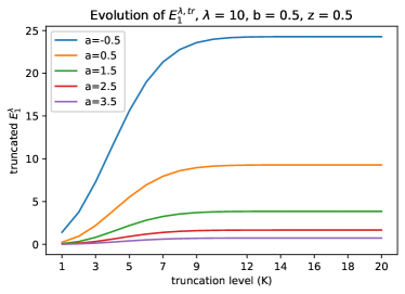
(a)

(b)

(c)

(d)

Figure 19: Evolution of ${E}^{\lambda,tr}_{i}$ for $i\in[2]$ and for various truncation levels ($K$).

Remarks:

• Since the first two arguments of the beta and incomplete beta functions are positive, these functions are bounded by $1$ and the ratio $\frac{\lambda^{K+1}}{(K+1)!}$ drives the error bounds $\mathcal{E}^{tr}_{1}$ and $\mathcal{E}^{tr}_{2}$. By the Stirling formula $(K+1)!=\mathcal{O}\left((K+1)^{\left(K+\frac{3}{2}\right)}\right)$. This means that to control $\mathcal{E}^{tr}_{1}$ and $\mathcal{E}^{tr}_{2}$, $K$ should be chosen at least of the same order of magnitude than $\lambda$.

• We show in Fig. 19 the evolution of ${E}^{\lambda,tr}_{1}$ and ${E}^{\lambda,tr}_{2}$ for different values of $\lambda$ and $a$ as a function of the level of truncation $K$. As anticipated in the previous remark, the sum starts to converge for $K$ of the same order of magnitude of $\lambda$. The function ${E}^{\lambda,tr}_{2}$ takes a few more iterations to converge.

Proof B.2.

(Lemma B.1) For $z\in[0,1]$, $a>-1$ and $b>-1$, let

$$E_{1}^{\lambda}(z,a,b) =\int_{0}^{z}y^{a}(1-y)^{b}e^{\lambda y}\mathrm{d}y,\quad E_{2}^{\lambda}(z,a,b)=\int_{z}^{1}y^{a}(1-y)^{b}e^{-\lambda y}\mathrm{d}y.$$

The infinite sum formulations follow from the exponential series expansions $e^{\lambda y}=\sum_{k=0}^{\infty}\frac{(\lambda y)^{k}}{k!}$ and $e^{-\lambda y}=\sum_{k=0}^{\infty}\frac{(-\lambda y)^{k}}{k!}$:

$$E_{1}^{\lambda}(z,a,b) =\int_{0}^{z}y^{a}(1-y)^{b}e^{\lambda y}\mathrm{d}y=\int_{0}^{z}y^{a}(1-y)^{b}\sum_{k=0}^{\infty}\frac{(\lambda y)^{k}}{k!}\mathrm{d}y=\sum_{k=0}^{\infty}\frac{\lambda^{k}}{k!}\underbrace{\int_{0}^{z}y^{a+k}(1-y)^{b}\mathrm{d}y}_{B_{\text{inc}}\left(a+k+1,b+1,z\right)},$$

$$E_{2}^{\lambda}(z,a,b) =\int_{z}^{1}y^{a}(1-y)^{b+1}e^{-\lambda y}\mathrm{d}y=\sum_{k=0}^{\infty}\frac{(-\lambda)^{k}}{k!}{\int_{z}^{1}y^{a+k}(1-y)^{b}\mathrm{d}y}$$

$$=\sum_{k=0}^{\infty}\frac{(-\lambda)^{k}}{k!}\Bigg{[}\underbrace{\int_{0}^{1}y^{a+k}(1-y)^{b}\mathrm{d}y}_{B\left(a+k+1,b+1\right)}-\underbrace{\int_{0}^{z}y^{a+k}(1-y)^{b}\mathrm{d}y}_{B_{\text{inc}}\left(a+k+1,b+1,z\right)}\Bigg{]}.$$

Let us now fix $K\in\mathbb{N}$, and truncate $E_{1}^{\lambda}(z,a,b)$ and $E_{2}^{\lambda}(z,a,b)$ to the first $K+1$ terms:

$$E_{1}^{\lambda,tr} =\sum_{k=0}^{K}\frac{\lambda^{k}}{k!}B_{\text{inc}}\left(a+k+1,b+1,z\right),$$

$$E_{2}^{\lambda,tr} =\sum_{k=0}^{K}\frac{(-\lambda)^{k}}{k!}\left[{B\left(a+k+1,b+1\right)}-{B_{\text{inc}}\left(a+k+1,b+1,z\right)}\right].$$

By the Taylor-Lagrange theorem, in case of

• $E_{1}^{\lambda}$: for any $y\in[0,z]$ there is a $y_{K}\in(0,y)$ such that $e^{\lambda y}=\sum_{k=0}^{K}\frac{(\lambda y)^{k}}{K!}+e^{\lambda y_{K}}\frac{(\lambda y)^{K+1}}{(K+1)!}.$

• $E_{2}^{\lambda}$: for any $y\in[z,1]$ there is a $y_{K}^{\prime}\in(0,y)$ such that $e^{-\lambda y}=\sum_{k=0}^{K}\frac{(-\lambda y)^{k}}{K!}+e^{-\lambda y^{\prime}_{K}}\frac{(-\lambda y)^{K+1}}{(K+1)!}.$

Hence, the truncation errors can be bounded as

$$E_{1}^{\lambda}-E_{1}^{\lambda,tr} =\int_{0}^{z}y^{a}(1-y)^{b}e^{\lambda y_{K}}\frac{(\lambda y)^{K+1}}{(K+1)!}\mathrm{d}y\stackrel{{\scriptstyle(a)}}{{\leq}}\int_{0}^{z}y^{a}(1-y)^{-1/2}e^{\lambda z}\frac{(\lambda y)^{K+1}}{(K+1)!}\mathrm{d}y$$

$$=\frac{\lambda^{K+1}e^{\lambda z}}{(K+1)!}\underbrace{\int_{0}^{z}y^{a+K+1}(1-y)^{b}\mathrm{d}y}_{B_{\text{inc}}\left(a+K+2,b+1,z\right)},$$

$$E_{21}^{\lambda}-E_{21}^{\lambda,tr} =\int_{z}^{1}y^{a}(1-y)^{b}e^{-\lambda y^{\prime}_{K}}\frac{(-\lambda y)^{K+1}}{(K+1)!}\mathrm{d}y\stackrel{{\scriptstyle(b)}}{{\leq}}\int_{z}^{1}y^{a}(1-y)^{b}e^{-\lambda z}\frac{(-\lambda y)^{K+1}}{(K+1)!}\mathrm{d}y$$

$$=\frac{(-\lambda)^{K+1}}{(K+1)!}e^{-\lambda z}\int_{z}^{1}y^{a+K+1}(1-y)^{b}\mathrm{d}y$$

$$=\frac{(-\lambda)^{K+1}}{(K+1)!}e^{-\lambda z}\left[\underbrace{\int_{0}^{1}y^{a+K+1}(1-y)^{b}\mathrm{d}y}_{B\left(a+K+2,b+1\right)}-\underbrace{\int_{0}^{z}y^{a+K+1}(1-y)^{b}\mathrm{d}y}_{B_{\text{inc}}\left(a+K+2,b+1,z\right)}\right]$$

$$=\frac{(-\lambda)^{K+1}}{(K+1)!}e^{-\lambda z}\left[B\left(a+K+2,b+1\right)-B_{\text{inc}}\left(a+K+2,b+1,z\right)\right],$$

where in (a) we used that $e^{\lambda y_{K}}\leq e^{\lambda z}$ and in (b) that $e^{-\lambda y^{\prime}_{K}}\leq e^{-\lambda z}$.

B.2 Score functions and kernel derivatives

The KSD and FSSD measures (see (9) and (10)) and their empirical counterparts rely on the functions $\xi_{q}$ and $h_{q}$ functions which can be readily obtained from the score function $s_{q}(x)$, kernel $K(x,y)$ and the associated derivatives $\frac{\partial K(x,y)}{\partial x}$ and $\frac{\partial^{2}K(x,y)}{\partial x\partial y}$. Table 10 and Table 11 provide these ingredients.

Distribution	$q(x)$	$s_{q}(x)$	Parameters
Gaussian	$\frac{1}{\sqrt{2\pi\sigma^{2}}}e^{-\frac{\left(x-m\right)^{2}}{2\sigma^{2}}}$	$-\frac{x-m}{\sigma^{2}}$	$m\in\mathbb{R},\sigma\in\mathbb{R}^{+}$
GN	$\frac{2^{-\frac{\gamma+1}{\gamma}}\gamma}{\beta\Gamma(1/\gamma)}e^{-\frac{1}{2}\left(\frac{\lvert x-\alpha\rvert}{\beta}\right)^{\gamma}}$	$-\frac{\gamma|x-\alpha|^{\gamma-1}}{2\beta^{\gamma}}\operatorname{sign}{x-\alpha}$	$\beta,\gamma\in\mathbb{R}^{+}$, $\alpha\in\mathbb{R}$
SG	$2(2\pi v)^{-1/2}e^{-\frac{(x-m)^{2}}{2v}}\Phi\left(\frac{s(x-m)}{\sqrt{v}}\right)$	$-\frac{x-m}{v}+\frac{e^{-\frac{s(x-m)}{\sqrt{v}}}}{\Phi\left(\frac{s(x-m)}{\sqrt{v}}\right)}\frac{s}{\sqrt{2\pi v}}$	$s,m\in\mathbb{R}$, $v\in\mathbb{R}^{+}$
beta	$\frac{1}{B(\alpha,\beta)}x^{\alpha-1}(1-x)^{\beta-1}\mathbb{I}_{[0,1]}(x)$	$\left(\frac{\alpha-1}{x}+\frac{\beta-1}{x-1}\right)\mathbb{I}_{[0,1]}(x)$	$\alpha,\beta\in\mathbb{R}^{+}$

Table 10: Distributions and their score functions.

Kernel	$K(x,y)$	$\frac{\partial K(x,y)}{\partial x}$	$\frac{\partial^{2}K(x,y)}{\partial x\partial y}$	Parameters
Gaussian	$e^{-\frac{(x-y)^{2}}{2{c}^{2}}}$	$e^{-\frac{(x-y)^{2}}{2{c}^{2}}}\left(-\frac{x-y}{{c}^{2}}\right)$	$e^{-\frac{(x-y)^{2}}{2{c}^{2}}}\left[-\frac{(x-y)^{2}}{{c}^{4}}+\frac{1}{{c}^{2}}\right]$	${c}\in\mathbb{R}^{+}$
Laplacian	$e^{-\lambda|x-y|}$	$e^{-\lambda|x-y|}\left[-\lambda\operatorname{sign}{x-y}\right]$	$-\lambda^{2}e^{-\lambda|x-y|}$	$\lambda\in\mathbb{R}^{+}$

Table 11: Kernels and their derivatives.

B.3 Moments of various distributions

Table 12 contains moments expressed as a function of the parameters for various target distributions.

Distribution ($\mathbb{Q}$)	$m_{\mathbb{Q}}$	$\sigma^{2}_{\mathbb{Q}}$	$\zeta_{\mathbb{Q}}$	$\kappa_{\mathbb{Q}}$
Gaussian	$m$	$\sigma^{2}$	0	0
GN	$\alpha$	$\beta^{2}4^{1/\gamma}\frac{\Gamma(3/\gamma)}{\Gamma(1/\gamma)}$	0	$\frac{\Gamma(5/\gamma)\Gamma(1/\gamma)}{\Gamma(3/\gamma)^{2}}-3$
SG	$m+\delta\sqrt{\frac{2v}{\pi}}$	$v\left(1-\frac{2\delta^{2}}{\pi}\right)$	$\frac{4-\pi}{2}\frac{\left(\delta{\sqrt{2/\pi}}\right)^{3}}{\left(1-2\delta^{2}/\pi\right)^{3/2}}$	$2(\pi-3)\frac{\left(\delta{\sqrt{2/\pi}}\right)^{4}}{\left(1-2\delta^{2}/\pi\right)^{2}}$
beta	$\frac{\alpha}{\alpha+\beta}$	$\frac{\alpha\beta}{(\alpha+\beta)^{2}(\alpha+\beta+1)}$	$2\frac{(\beta-\alpha){\sqrt{\alpha+\beta+1}}}{(\alpha+\beta+2){\sqrt{\alpha\beta}}}$	$6\frac{(\beta-\alpha)^{2}(\alpha+\beta+1)-\alpha\beta(\alpha+\beta+2)}{\alpha\beta(\alpha+\beta+2)(\alpha+\beta+3)}$

Table 12: Moments of the target distributions.

Appendix C External statements

This section contains external statements used in our proofs.

Lemma C.1 (Generalized Markov’s inequality; (2.1) in [4]).

Let $\phi$ denote a nondecreasing and nonnegative function defined on $I\subseteq\mathbb{R}$ and let $Y$ denote a random variable taking values in $I$. Then Markov’s inequality implies that for every $t\in I$ with $\phi(t)>0$

$$\mathbb{P}\left(Y\geq t\right)\leq\frac{\mathbb{E}\phi(Y)}{\phi(t)}.$$

Theorem C.2 (Hoeffding inequality for U-statistic; [25], [47]).

Assume that we have $n$ i.i.d. samples $\{X_{i}\}_{i\in[n]}\sim\mathbb{P}$. Let $I_{m}^{n}$ be the set $m$-tuples chosen without repetition from $[n]$. Suppose that $h:\mathbb{R}^{m}\rightarrow\mathbb{R}$ is bounded: $a\leq h(x_{1},\dots,x_{m})\leq b$ for all $(x_{1},\dots,x_{m})$. We denote $m_{h}=\mathbb{E}h(X_{1},\dots,X_{m})$ and its U-statistic based estimator $U_{n}=\frac{1}{\binom{n}{m}}\sum_{(i_{1},\dots,i_{m})\in I_{m}^{n}}h(X_{i_{1}},\dots,X_{i_{m}})$. Then, for any $\varepsilon>0$

$$\mathbb{P}\left(U_{n}-m_{h}>\varepsilon\right)\leq e^{-\frac{2\left\lfloor\frac{n}{m}\right\rfloor\varepsilon^{2}}{(b-a)^{2}}},$$

and the same deviation bound holds for $-\varepsilon$ below, i.e. $\mathbb{P}\left(U_{n}-m_{h}<-\varepsilon\right)\leq e^{-\frac{2\left\lfloor\frac{n}{m}\right\rfloor\varepsilon^{2}}{(b-a)^{2}}}$.

Theorem C.3 (Burkholder’s inequality; Theorem 2.10 in [23]).

Assume that $\{(S_{i},\mathcal{F}_{i})\}_{i\in[n]}$ is a martingale sequence and its filtration, $1<p<\infty$. Let the associated martingale increments be denoted by $X_{1}=S_{1}$ and $X_{i}=S_{i}-S_{i-1},2\leq i\leq n$. Then there exist a constant $C_{p}$ depending on $p$ such that

$$\mathbb{E}{\bigg{\lvert}S_{n}\bigg{\rvert}^{p}}\leq C_{p}\mathbb{E}{\bigg{\lvert}\sum_{i=1}^{n}X_{i}^{2}\bigg{\rvert}^{p/2}}.$$

Lemma C.4 (Kullback-Leibler divergence for univariate Gaussian variables; page 13 in [10]).

Let $\mathbb{P}=\mathcal{N}(m_{\mathbb{P}},\sigma_{\mathbb{P}})$, $\mathbb{Q}=\mathcal{N}(m_{\mathbb{Q}},\sigma_{\mathbb{Q}})$, $m_{\mathbb{P}},m_{\mathbb{Q}}\in\mathbb{R}$, $\sigma_{\mathbb{P}},\sigma_{\mathbb{Q}}\in\mathbb{R}^{>0}$. Then

$$D_{\text{KL}}\left(\mathbb{P},\mathbb{Q}\right) =\log\left(\frac{\sigma_{\mathbb{Q}}}{\sigma_{\mathbb{P}}}\right)+\frac{\sigma_{\mathbb{P}}^{2}+(m_{\mathbb{Q}}-m_{\mathbb{P}})^{2}}{2\sigma_{\mathbb{Q}}^{2}}-\frac{1}{2}.$$

Theorem C.5 (Theorem 2.2 in [57]).

Let $\mathscr{X}$ and $\Theta$ denote two measurable spaces. Let $F:\Theta\rightarrow\mathbb{R}$ be a functional. Let $\mathcal{P}_{\Theta}=\{\mathbb{P}_{\theta}\,:\,\theta\in\Theta\}$ be a class of probability measures on $\mathscr{X}$ indexed by $\Theta$. We observe the data $D$ distributed according $\mathbb{P}_{\theta}\in\mathcal{P}_{\Theta}$ with some unknown $\theta$. The goal is to estimate $F(\theta)$. Let $\hat{F}:=\hat{F}(D)$ be an estimator of $F(\theta)$ based on $D$. Assume that there exist $\theta_{0},\theta_{1}\in\Theta$ such that $|F(\theta_{0})-F(\theta_{1})|\geq 2s>0$ and $D_{\text{KL}}\left(\mathbb{P}_{\theta_{1}},\mathbb{P}_{\theta_{0}}\right)\leq\alpha$ with $0<\alpha<\infty$. Then

$$\inf_{\hat{F}}\sup_{\theta\in\Theta}\mathbb{P}_{\theta}\left(|\hat{F}-F(\theta)|\geq s\right)\geq\max\left(\frac{e^{-\alpha}}{4},\frac{1-\sqrt{\alpha/2}}{2}\right).$$

Note: Typically $\mathscr{X}$, $D$ and $\mathbb{P}_{\theta}$ depend on the sample size $N$.

References

- [1] K. Balasubramanian, T. Li, and M. Yuan, On the optimality of kernel-embedding based goodness-of-fit tests, Journal of Machine Learning Research, 22 (2021), pp. 1–45.
- [2] A. Berlinet and C. Thomas-Agnan, Reproducing Kernel Hilbert Spaces in Probability and Statistics, Kluwer, 2004.
- [3] M. Binkowski, D. Sutherland, M. Arbel, and A. Gretton, Demystifying MMD GANs, in International Conference on Learning Representations (ICLR), 2018.
- [4] S. Boucheron, G. Lugosi, and P. Massart, Concentration inequalities, Oxford University Press, 2013.
- [5] L. Boudabsa and D. Filipović, Machine learning with kernels for portfolio valuation and risk management, tech. report, EPFL, 2019. (Swiss Finance Institute Research Paper No. 19-34; https://dx.doi.org/10.2139/ssrn.3401539).
- [6] F.-X. Briol, A. Barp, A. B. Duncan, and M. Girolami, Statistical inference for generative models with maximum mean discrepancy, tech. report, 2019. (https://arxiv.org/abs/1906.05944).
- [7] Y. Chalabi and D. Wuertz, Portfolio optimization based on divergence measures, tech. report, 2012. (https://mpra.ub.uni-muenchen.de/43332/).
- [8] K. Chwialkowski, H. Strathmann, and A. Gretton, A kernel test of goodness of fit, in International Conference on Machine Learning (ICML), 2016, pp. 2606–2615.
- [9] R. Cont, Empirical properties of asset returns: Stylized facts and statistical issues, Quantitative Finance, 1 (2001), pp. 223–236.
- [10] J. Duchi, Derivations for linear algebra and optimization, tech. report, The University of Stanford, 2007. (https://web.stanford.edu/~jduchi/projects/general_notes.pdf).
- [11] G. K. Dziugaite, D. M. Roy, and Z. Ghahramani, Training generative neural networks via maximum mean discrepancy optimization, in Conference on Uncertainty in Artificial Intelligence (UAI), 2015, pp. 258–267.
- [12] F. J. Fabozzi, P. N. Kolm, D. Pachamanova, and S. M. Focardi, Robust portfolio optimization and management, John Wiley & Sons, 2012.
- [13] K. R. French, Data Library, 2021. (https://mba.tuck.dartmouth.edu/pages/faculty/ken.french/data_library.html).
- [14] K. Fukumizu, A. Gretton, X. Sun, and B. Schölkopf, Kernel measures of conditional dependence, in Advances in Neural Information Processing Systems (NIPS), 2008, pp. 498–496.
- [15] W. Gong, Y. Li, and J. M. Hernández-Lobato, Sliced kernelized Stein discrepancy, tech. report, 2020. (https://arxiv.org/abs/2006.16531).
- [16] J. Gorham and L. Mackey, Measuring sample quality with Stein’s method, in Advances in Neural Information Processing Systems (NIPS), 2015, pp. 226–234.
- [17] J. Gorham and L. Mackey, Measuring sample quality with kernels, in International Conference on Machine Learning (ICML), 2017, pp. 1292–1301.
- [18] J. Gorham, A. Raj, and L. Mackey, Stochastic Stein discrepancies, in Advances in Neural Information Processing Systems (NeurIPS), 2020, pp. 17931–17942.
- [19] W. Grathwohl, K.-C. Wang, J.-H. Jacobsen, D. Duvenaud, and R. Zemel, Learning the Stein discrepancy for training and evaluating energy-based models without sampling, in International Conference on Machine Learning (ICML), 2020, pp. 3732–3747.
- [20] A. Gretton, K. Borgwardt, M. Rasch, B. Schölkopf, and A. Smola, A kernel two-sample test, Journal of Machine Learning Research, 13 (2012), pp. 723–773.
- [21] A. Gretton, K. Fukumizu, C. H. Teo, L. Song, B. Schölkopf, and A. Smola, A kernel statistical test of independence, in Advances in Neural Information Processing Systems (NIPS), 2008, pp. 585–592.
- [22] I. Guo, N. Langrené, G. Loeper, and W. Ning, Portfolio optimization with a prescribed terminal wealth distribution, tech. report, 2020. (https://arxiv.org/abs/2009.12823).
- [23] P. Hall and C. C. Heyde, Martingale Limit Theory and its Application, Academic Press, 1980.
- [24] Z. Harchaoui, F. Bach, and E. Moulines, Testing for homogeneity with kernel Fisher discriminant analysis, in Advances in Neural Information Processing Systems (NIPS), 2007, pp. 609–616.
- [25] W. Hoeffding, Probability inequalities for sums of bounded random variables, Journal of the American Statistical Association, 58 (1963), pp. 13–30.
- [26] J. H. Huggins and L. Mackey, Random feature Stein discrepancies, in Advances in Neural Information Processing Systems (NeurIPS), 2018, pp. 1899–1909.
- [27] R. Jagannathan and T. Ma, Risk reduction in large portfolios: Why imposing the wrong constraints helps, The Journal of Finance, 58 (2003), pp. 1651–1683.
- [28] W. Jitkrittum, W. Xu, Z. Szabó, K. Fukumizu, and A. Gretton, A linear-time kernel goodness-of-fit test, in Advances in Neural Information Processing Systems (NIPS), 2017, pp. 261–270.
- [29] P. Jorion, Bayes-Stein estimation for portfolio analysis, Journal of Financial and Quantitative Analysis, 21 (1986), pp. 279–292.
- [30] M. Kennedy, Bayesian quadrature with non-normal approximating functions, Statistics and Computing, 8 (1998), pp. 365–375.
- [31] B. Kim, R. Khanna, and O. Koyejo, Examples are not enough, learn to criticize! criticism for interpretability, in Advances in Neural Information Processing Systems (NIPS), 2016, pp. 2280–2288.
- [32] W. C. Kim, F. J. Fabozzi, P. Cheridito, and C. Fox, Controlling portfolio skewness and kurtosis without directly optimizing third and fourth moments, Economics Letters, 122 (2014), pp. 154–158.
- [33] N. Lassance, Information-theoretic approaches to portfolio selection, PhD thesis, Louvain School of Management, 2019.
- [34] O. Ledoit and M. Wolf, Improved estimation of the covariance matrix of stock returns with an application to portfolio selection, Journal of Empirical Finance, 10 (2003), pp. 602–621.
- [35] Y. Li, K. Swersky, and R. Zemel, Generative moment matching networks, in International Conference on Machine Learning (ICML), 2015, pp. 1718–1727.
- [36] Q. Liu, J. Lee, and M. Jordan, A kernelized Stein discrepancy for goodness-of-fit tests, in International Conference on Machine Learning (ICML), 2016, pp. 276–284.
- [37] J. R. Lloyd, D. Duvenaud, R. Grosse, J. Tenenbaum, and Z. Ghahramani, Automatic construction and natural-language description of nonparametric regression models, in AAAI Conference on Artificial Intelligence, 2014, pp. 1242–1250.
- [38] H. Markowitz, Portfolio selection, The Journal of Finance, 7 (1952), pp. 77–91.
- [39] L. Martellini and V. Ziemann, Improved estimates of higher-order comoments and implications for portfolio selection, The Review of Financial Studies, 23 (2010), pp. 1467–1502.
- [40] R. C. Merton, Optimum consumption and portfolio rules in a continuous-time model, Journal of Economic Theory, 3 (1971), pp. 373–413.
- [41] J. Mooij, J. Peters, D. Janzing, J. Zscheischler, and B. Schölkopf, Distinguishing cause from effect using observational data: Methods and benchmarks, Journal of Machine Learning Research, 17 (2016), pp. 1–102.
- [42] A. Müller, Integral probability metrics and their generating classes of functions, Advances in Applied Probability, 29 (1997), pp. 429–443.
- [43] C. J. Oates, J. Cockayne, F.-X. Briol, and M. Girolami, Convergence rates for a class of estimators based on Stein’s method, Bernoulli, 25 (2019), pp. 1141–1159.
- [44] C. J. Oates, M. Girolami, and N. Chopin, Control functionals for Monte Carlo integration, Journal of the Royal Statistical Society: Series B, 79 (2017), pp. 695––718.
- [45] G. Peyré and M. Cuturi, Computational optimal transport, Foundations and Trends in Machine Learning, 11 (2019), pp. 355–607.
- [46] N. Pfister, P. Bühlmann, B. Schölkopf, and J. Peters, Kernel-based tests for joint independence, Journal of the Royal Statistical Society: Series B (Statistical Methodology), 80 (2018), pp. 5–31.
- [47] Y. Pitcan, A Note on Concentration Inequalities for U-Statistics, tech. report, University of Berkeley, 2017. (https://arxiv.org/abs/1712.06160).
- [48] R. Y. Rubinstein and D. P. Kroese, The cross-entropy method: A unified approach to combinatorial optimization, Monte-Carlo simulation, and machine learning, Springer, 2004.
- [49] R. C. Scott and P. A. Horvath, On the direction of preference for moments of higher order than the variance, The Journal of finance, 35 (1980), pp. 915–919.
- [50] A. Smola, A. Gretton, L. Song, and B. Schölkopf, A Hilbert space embedding for distributions, in Algorithmic Learning Theory (ALT), 2007, pp. 13–31.
- [51] L. Song, X. Zhang, A. Smola, A. Gretton, and B. Schölkopf, Tailoring density estimation via reproducing kernel moment matching, in International Conference on Machine Learning (ICML), 2008, p. 992–999.
- [52] L. F. South, T. Karvonen, C. Nemeth, M. Girolami, and C. J. Oates, Semi-exact control functionals from Sard’s method, tech. report, 2020. (https://arxiv.org/abs/2002.00033).
- [53] B. Sriperumbudur, K. Fukumizu, and G. Lanckriet, Universality, characteristic kernels and RKHS embedding of measures, Journal of Machine Learning Research, 12 (2011), pp. 2389–2410.
- [54] B. Sriperumbudur, A. Gretton, K. Fukumizu, B. Schölkopf, and G. Lanckriet, Hilbert space embeddings and metrics on probability measures, Journal of Machine Learning Research, 11 (2010), pp. 1517–1561.
- [55] Z. Szabó, Information theoretical estimators toolbox, Journal of Machine Learning Research, 15 (2014), pp. 283–287.
- [56] I. Tolstikhin, B. Sriperumbudur, and B. Schölkopf, Minimax estimation of maximal mean discrepancy with radial kernels, in Advances in Neural Information Processing Systems (NIPS), 2016, pp. 1930–1938.
- [57] A. B. Tsybakov, Introduction to nonparametric estimation, Springer, 2009.
- [58] C. Villani, Optimal Transport: Old and New, Springer, 2008.
- [59] M. Yamada, Y. Umezu, K. Fukumizu, and I. Takeuchi, Post selection inference with kernels, in International Conference on Artificial Intelligence and Statistics (AISTATS), 2018, pp. 152–160.
- [60] V. Zolotarev, Probability metrics, Theory of Probability and its Applications, 28 (1983), pp. 278–302.