No RL, No Simulation: Learning to Navigate without Navigating

Abstract

Most prior methods for learning navigation policies require access to simulation environments, as they need online policy interaction and rely on ground-truth maps for rewards. However, building simulators is expensive (requires manual effort for each and every scene) and creates challenges in transferring learned policies to robotic platforms in the real-world, due to the sim-to-real domain gap. In this paper, we pose a simple question: Do we really need active interaction, ground-truth maps or even reinforcement-learning (RL) in order to solve the image-goal navigation task? We propose a self-supervised approach to learn to navigate from only passive videos of roaming. Our approach, No RL, No Simulator (NRNS), is simple and scalable, yet highly effective. NRNS outperforms RL-based formulations by a significant margin. We present NRNS as a strong baseline for any future image-based navigation tasks that use RL or Simulation.

1 Introduction

In recent years, we have seen significant advances in learning-based approaches for indoor navigation [1, 2]. Impressive performance gains have been obtained for a range of tasks, from non-semantic point-goal navigation [3] to semantic tasks such as image-goal [4] and object-goal navigation [5, 6], via methods that use reinforcement learning (RL). The effectiveness of RL for these tasks can be attributed in part to the emergence of powerful new simulators such as Habitat [7], Matterport [8] and AI2Thor [9]. These simulators have helped scale learning to billions of frames by providing large-scale active interaction data and ground-truth maps for designing reward functions. But do we actually need simulation and RL to learn to navigate? Is there an alternative way to formulate the navigation problem, such that no ground-truth maps or active interaction are required? These are valuable questions to explore because learning navigation in simulation constrains the approach to a limited set of environments, since the creation of 3D assets remains costly and time-consuming.

In this paper, we propose a self-supervised approach to learning how to navigate from passive egocentric videos. Our novel method is simple and scalable (no simulator required for training), and at the same time highly effective, as it outperforms RL-based formulations by a significant margin. To introduce our approach, let us first examine the role of RL and simulation in standard navigation learning methods. In the standard RL formulation, an agent gets a reward upon reaching the goal, followed by a credit assignment stage to determine the most useful state-action pairs. But do we actually need the reinforce function for action credit assignment? Going a step further, do we even need to learn a policy explicitly? In navigation, we argue that the state space itself is highly structured via a distance function, and the structure itself could be leveraged for credit assignment. Simply put, states that help reduce the distance to the goal are better – and therefore predicted distance can be used either as the value function or as a proxy for it. In fact, RL formulations frequently use ‘distance reduced to goal’ in reward shaping. The key property of our approach is that we learn a generalizable distance estimator directly from passive videos, and as a result we do not require any interaction. We demonstrate that an effective distance estimator can be learned directly from visual trajectories, without the need for an RL policy to map visual observations to the action space, thereby obviating the need for extensive interaction in a simulator and hand-designed rewards. However passive videos do not provide learning opportunities for obstacle avoidance since they rarely, if ever, consist of cameras bumping into walls. We forgo the need for active interaction to reason about collisions as we show that obstacle avoidance is only required locally and simple depth maps are sufficient to prune invalid actions and locations for navigation. More broadly, our approach can be considered as closely related to model-based control, which is an alternative paradigm to RL-based policy learning, with the key insight that components of the model and cost functions can be learned from passive data.

No RL, No Simulator Approach (NRNS): Our NRNS algorithm can be described as follows. During training we learn two functions from passive videos: (a) a geodesic distance estimator: given the state features and goal image, this function predicts the geodesic distance of the unexplored frontiers of the graph to the goal location. This enables a greedy policy in which we select the node with the least distance; (b) a target prediction model: Given the goal image and the image from the agent’s current location, this function predicts if the goal is within sight and can be reached without collisions, along with the exact location of the goal. The key is that both the distance model and the target prediction model can be learned from passive RGBD videos, with SLAM used to estimate relative poses. We believe our simple NRNS approach should act as a strong baseline for any future approaches that use RL and simulation. We show that NRNS outperforms end-to-end RL, even when RL is trained using 5x more data and 10x more compute. Furthermore, unlike RL methods which need to be trained in simulation because they require substantial numbers of interactions, NRNS can be trained directly on real-world videos alone, and therefore does not suffer from the sim-to-real gap.

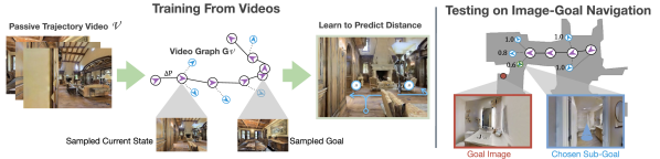
Figure 1: Left: Using passive videos we learn to predict distances for navigation. Our distance function learns the priors of the layouts of indoor buildings to estimate distances to goal location. Right: Image-Goal Navigation Task [10]. Our model uses distance function to predict distances of unexplored nodes and uses greedy policy to choose the shortest-distance node.

2 Related Work

Navigation in simulators. Navigation tasks largely fall into two main categories [1], ones in which a goal location is known [11, 12, 13] and limited exploration is required, and ones in which the goal location is not known and efficient exploration is necessary. In the second category, tasks range from finding the location of specific objects [5], rooms [14], or images  [15], to the task of exploration itself [2]. The majority of current work [12, 15, 16, 3] leverages simulators [7] and extensive interaction to learn end-to-end models for these tasks. In contrast, our work shows that the semantic cues needed for exploration-based navigation tasks can be learned directly from video trajectories.

Navigation using passive data. Several prior works have tackled the navigation task when there is some passive experience available in the test environment [17, 18, 19, 20, 21, 22]. A more limited number of works train navigation policies without simulation environments [19, 22, 23]. Unlike these works, we tackle the task of image goal navigation in unseen environments where there is no experience available to the agent in the test environments during training [19, 22] and no map knowledge is given about the environments [23]. Two works adopting similar requirements are Chaplot et al. [4] and Chang et al. [24]. Most closely related is Neural Topological SLAM (NTS) [4], which builds a topological map and estimates distance to the target image using a learned function. But NTS requires access to panoramic observations and ground-truth maps for training the distance function, making it much less scalable than our approach which can be trained with just video data with arbitrary field of view. Chang et al. [24] adopt a similar approach to NTS for object goal navigation, while also incorporating video data from YouTube for learning a Q function. A key difference is that our method learns a episodic distance function, utilizing all past observations to estimate distances to the target image. In comparison, Chaplot et al. [4] and Chang et al. [24] use a memory-less distance function operating only on the agent’s current observation.

Prior work work on LfD [25, 26, 27] requires: (a) access to actions (e.g. teleoperated in simulator); and (b) optimal human demonstrations. The goal in LfD is to learn policies that match given demonstrations by either mimicking the actions or formulating rewards using the demonstrations. In contrast, NRNS does neither, since our passive training data does always contain optimal navigation trajectories and NRNS does not compute any rewards as it does not require RL or credit assignment. We make the same distinction between our work and offline RL [28, 29, 30], which does not utilize online data gathering but still learns a policy using rewards from observed trajectories. In contrast, we do not use any rewards or learn a policy. Instead, our approach aims to learn a distance-to-goal model and uses a greedy policy based on the distance predictions. From this perspective, NRNS is performing model-based learning.

Map-Based Navigation. There are multiple spatial representations which can be leveraged in solving navigation tasks. Metric maps, which maintain precise information on the occupied space in an environment, are commonly used for visual navigation [2, 10, 6]. However, metric maps suffer from issues of scalability and consistency under sensor noise. As a result, topological maps have recently gained traction [4, 21, 18, 24, 31] as a means to combat these issues. A significant difference from our approach is that in these prior works a topological map is given at the beginning of the navigation task, and is not created or changed during navigation. Specifically, Savinov et al. [18] create the map from a given 5 minute video of the test environment and Chen et al. [21] assume access to a ground truth map. In our image-goal navigation set up, the agent is given no information about the test environment. Chaplot et al. [4] do not require experience in the test environment and build topological maps at test time, but still requires access to a simulator for computing shortest-path distances between pairs of images. Additionally, topological maps for robotic navigation draw inspiration from both animal and human psychology. The cognitive map hypothesis proposes that the brain builds coarse internal spatial representations of environments [32, 33]. Multiple works argue that this internal representation relies on landmarks [34, 35], making human cognitive maps more similar to topological maps as opposed to metric maps.

Graph Neural Networks. Graph Neural Networks (GNN) are specifically used for modeling relational data in a non-Euclidean space. We employ a GNN for estimating distance-to-goal over the agent’s exploration frontier. Specifically we employ an augmented Graph Attention Network [36] which allows for a weighted aggregation of neighboring node information. Graph Networks are rarely-used for the task of topological map-based visual navigation. Savinov et al. [18] use a GNN for the sub-task of localizing the agent in a ground truth topological map. We believe we are the first to leverage graph neural networks in a visual navigation task.

3 Image Goal Navigation using Topological Graphs

We propose No RL, No Simulator “NRNS”, a hierarchical modular approach to image-goal navigation that consists of: a) high-level modules for maintaining a topological map and using visual and semantic reasoning to predict sub-goals, and b) heuristic low-level modules that use depth data to select low level navigation actions to reach sub-goals and determine geometrically-explorable areas. We first describe NRNS in detail and then show in Sec. 4 that the high-level modules can be trained without using any simulation, interaction or even ground-truth scans – i.e. that passive video data alone is sufficient to learn the semantic and visual reasoning models needed for navigation.

3.1 Formulation and Representation

Task Definition. We tackle the task of image-goal navigation, where an agent is placed in a novel environment, and is tasked with navigating to an (unknown) goal position that is specified using an image taken from that position, as shown in Fig. 2. More formally, an episode begins with an agent receiving an RGB observation ($I_{G}$) corresponding to the goal position. At each time step, $t$, of the episode the agent receives a set of observations $s_{t}$, and must take a navigation action $a_{t}$. The agents state observations, $s_{t}$, are defined as a narrow field of view RGBD image, $I_{t}$, and egocentric pose estimate, $P_{t}$. The agent must execute navigational actions to reach goal within a maximum number of steps.

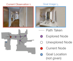
Figure 2: Image-Goal navigation task using a topological graph.

Topological Map Representation. The NRNS agent maintains a topological map in the form of a graph $G(N,E)$, defined by nodes $N$ and edges $E$, which provides a sparse representation of the environment. Concretely, a node $n_{i}\in N$ is associated with a pose $p_{i}$, defined by location and orientation. Each node $n_{i}$ can either be ‘explored’ i.e. the agent has previously visited the pose and obtained a corresponding RGBD image $I_{i}$, or ‘unexplored’ e.g. unvisited positions at the exploration frontier which may be visited in the future. Each edge $e\in E$ connects a pair of adjacent nodes $n_{i}$ and $n_{j}$. Nodes are deemed adjacent only if a short and ‘simple’ path exists between the two nodes, as further detailed in Sec. 3.3. Each edge between adjacent nodes is then associated with the attribute $\Delta P$ – the relative pose between the two nodes.

3.2 Global Policy via Distance Prediction

Given a representation of the environment as a topological graph, our global policy is tasked with identifying the next ‘unexplored’ node that the agent should visit, and the low-level policy ($\mathcal{G}_{LP}$) is then responsible for executing the precise actions. Intuitively, we want our agent to select as the next node the one that minimizes the total distance to goal. The global policy’s inference task can thus be reduced to predicting distances from nodes in our graph to the goal location. To this end, our approach leverages a distance prediction network ($\mathcal{G}_{D}$) which operates on top of $G(N,E)$ to predict distance-to-goal for each unexplored node $n_{ue}\in G$. Our global policy then simply selects the node with least total distance to goal which is defined as: distance to the unexplored node from the agent’s current position, plus the predicted distance from the unexplored node to the goal.

The input to the distance prediction network $\mathcal{G}_{D}$ is the current topological graph $G(N,E)_{t}$ and $I_{G}$. While the explored nodes have an image associated with them, the unexplored nodes naturally do not. To allow prediction in this setup, we use a Graph Convolutional Network (GCN) architecture to first induce visual features for $n_{ue}\in G$, and then predict the distance to goal using an MLP.

As illustrated in Fig. 3, the network first encodes the RGB images at each explored node ($n_{i}$) using a ResNet18 [37] to obtain feature vector $\mathbf{h_{i}}\in\mathbb{R}^{512}$. Each edge $e_{i,j}$ is further represented by a feature vector $\mathbf{u_{i,j}}$, which is the flattened pose transformation matrix ($\mathbf{{}^{i}K_{j}}\in\mathbb{R}^{4\times 4}$). The adjacency matrix $\mathbf{A_{t}}$, $\mathbf{u_{i,j}}$, and $\mathbf{h_{i}}$ are passed through a GCN comprising of two graph attention (GAT) layers [36] with intermediate nonlinearities. Note that we extend the graph attention layer architecture to additionally use edge features $\mathbf{u_{i,j}}$ when computing attention coefficients. The predicted visual features for unexplored nodes are then finally used to compute predicted distance-to-goal $d_{i}$ from each node to $I_{G}$ using a simple MLP.

To select the most ‘promising’ $n_{ue}$ to explore, the distance from the agent’s current location $n_{t}$ also needs to be accounted for. For $n_{ue},n_{t}\in G$, the ‘travel cost’ is added to $d_{i}$, calculated using shortest path on G from $n_{ue}\rightarrow n_{t}$. Our global policy then selects the unexplored node with the minimum total distance score as the next sub-goal.

3.3 Local Navigation and Graph Expansion

Figure 3: The Global Policy and $\mathcal{G}_{D}$ architecture used to model distance-to-goal prediction. $\mathcal{G}_{D}$ employs a Resnet18 encoder, Graph Attention layers, and a multi-layer perceptron with a sigmoid.

The NRNS global policy selects the sub-goal that the agent should pursue, and the precise low-level actions to reach the sub-goal are executed by a heuristic local policy. After the local policy finishes execution, the NRNS agent updates the graph to include the new observations and expands the graph with unexplored nodes at the exploration frontier.

Local Policy. The NRNS local policy, denoted as $\mathcal{G}_{LP}$, receives a target position, defined by distance and angle ($\rho_{i}$, $\phi_{i}$) with respect to the agent’s current location. When $\mathcal{G}_{D}$ outputs a sub-goal node, $\rho_{i}$, $\phi_{i}$ are calculated from the current position and passed to $\mathcal{G}_{LP}$. Low level navigation actions are selected and executed using a simplistic point navigation model based on the agent’s egocentric RGBD observations and (noisy) pose estimation. To navigate towards its sub-goal, the agent builds and maintains a local metric map using the noisy pose estimator and depth input. This effectively allows it to reach local goals and avoid obstacles. The local metric maps are discarded upon reaching the sub-goal, as they are based on a noisy pose estimator. This policy is adapted from [10] and is also used for Image-Goal Navigation in [4].

Explorable Area Prediction for Graph Expansion. We incorporate a ‘graph expansion’ step after the agent reaches a sub-goal via $\mathcal{G}_{LP}$ and before the agent selects a new sub-goal. First, the agent updates $G(N,E)$ to record the current location as an explored node and store the associated RGBD observation. Second, the agent creates additional ‘unexplored’ nodes, $n_{ue}$, adjacent to the current node, $n_{t}$ based on whether the corresponding directions are deemed ‘explorable’. We use a explorable area prediction module, $\mathcal{G}_{EA}$, to determine which adjacent areas to the current location are geometrically explorable. This is untrained, heuristic module takes the egocentric depth image $I_{t_{depth}}$ and tests 9 angles in the direction $\theta$ from the current position and returns the angles $\theta$ that are not blocked by obstacles within a depth of 3 meters. The NRNS agent tests $\theta$ at [0,$\pm$15,$\pm$30,$\pm$45,$\pm$60], these angles are chosen based on the agent’s turn radius of 15° and 120° FOV. For all $\theta$ determined to be explorable, the agent updates $G(N,E)$ by adding an ‘unexplored’ node at position $\rho=1m$ and $\phi=\theta$ relative to the node the agent is at, with a corresponding edge linking the current node to the new node. If a node already exists in one of the explorable areas at a nearby position, only an edge is added to $G(N,E)$ and not a new node.

3.4 Putting it Together

Stopping Criterion. The above described modules ($\mathcal{G}_{D}$, $\mathcal{G}_{LP}$, $\mathcal{G}_{EA}$) allow the NRNS agent to incrementally explore its environment while making progress towards the location of the target image. To allow the agent to terminate navigating when it is near the goal, we additionally learn a target prediction network $\mathcal{G}_{T}$ that provides a stopping criterion. Given $I_{G}$ and current image $I_{t}$, $\mathcal{G}_{T}$ is simple MLP that predicts: a) a probability $\beta_{s}\in[0,1]$ indicating whether the goal is within sight, and if so, b) the relative position (distance, direction) of the goal $\rho_{g}$, $\phi_{g}$.

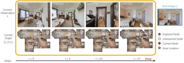
Figure 6: Example of an Image-Goal Navigation episode on MP3D. Shows the agent’s observations and internal topological graph at different time steps.

Algorithm. We outline our navigation algorithm in Fig. 4. An example result on the image-goal navigation task is shown in Fig. 6. Among the modules used, the local policy module $\mathcal{G}_{LP}$ and the explorable area module $\mathcal{G}_{EA}$ do not require any learning. As we show in Sec. 4, $\mathcal{G}_{D}$ and $\mathcal{G}_{T}$ can both be learned using only passive data.

// initialize graph

$n_{0}=(P_{t=0},I_{t=0});e_{0}=(n_{0},n_{0})$;

$N=(n_{0});E=(e_{0})$;

$G=(N,E)$;

// loop until reached goal or max steps

while steps taken < max steps do

       ${n_{i+1},...,n_{i+k}}=\text{$\mathcal{G}_{EA}$}(I_{t})$; // determine valid explorable areas

       $N\mathrel{+}={n_{i+1},...,n_{i+k}};E\mathrel{+}={e_{t,i+1},...,e_{t,i+k}}$; // add unexplored nodes & edges

       $n_{sg},(\rho_{sg},\phi_{sg})=\mathrm{argmin}(\text{$\mathcal{G}_{D}$}(G,I_{G})+\text{TravelCost}(G,n_{t}))$; // select sub-goal

       $I_{t+1},P_{t+1}=\text{$\mathcal{G}_{LP}$}(\rho_{sg},\phi_{sg})$; // navigate to sub-goal

       $n_{sg}=(P_{t+1},I_{t+1})$ // update graph with observations

       $\beta_{s},(\rho_{g},\phi_{g})=\text{$\mathcal{G}_{T}$}(I_{t+1},I_{G})$; // stopping criterion

       if $\beta_{s}$ > .5 then

             $\text{$\mathcal{G}_{LP}$}(\rho_{g},\phi_{g})$; // navigate to target

             break;

            

       end if

      

end while

Algorithm 1 NRNS Image Navigation

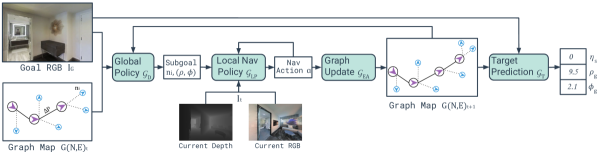
Figure 4: The hierarchical modular NRNS approach to the Image-Goal Navigation task, for a single time step in the episode. The global policy $\mathcal{G}_{D}$ selects an unexplored node $n_{i}$ as a sub-goal. The sub-goal position $(\rho_{i},\phi_{i})$ is passed to the local navigation policy $\mathcal{G}_{LP}$ which takes in the current RGBD observations and outputs low level actions until the agent reaches $n_{i}$. The graph is then updated with the current observations $I_{t+1}$ and new unexplored nodes and edges generated by $\mathcal{G}_{EA}$.

4 Learning from Passive Data

The learned high-level policies of NRNS are the Distance Network $\mathcal{G}_{D}$ and Target Prediction Network $\mathcal{G}_{T}$. A key contribution of our work is showing that these functions can be learned from passive data alone. This eliminates the need for online interaction and ground-truth maps, allowing us to train the NRNS algorithm without using RL or simulation.

Learning Distance Prediction. First, we describe how to learn the function $\mathcal{G}_{D}$. Given a topological graph (consisting of both explored and unexplored nodes) and a goal image as input, $\mathcal{G}_{D}$ predicts the geodesic distance from all unexplored nodes to the location of the goal image. Our training data therefore consists of triplets of the form $(G,I_{G},D_{U})$, where $G$ is a topological graph, $I_{G}$ is a goal image, and $D_{U}$ is the ground-truth distances from a set of unexplored nodes to the goal location (we use L2-Loss to train the distance function).

We generate training graphs using passive videos in a two-step process. In the first step, we create a topological graph, $G_{\mathcal{V}_{i}}$, for every video $\mathcal{V}_{i}$ in the passive dataset. Each graph contains both explored and unexplored nodes. We approximate distance to unexplored nodes using the geodesic distance along the trajectory. In the second step, we uniformly sample sub-graphs and goal locations over each video’s topological graph.

Step 1: Video to Topological Graph. First, we generate a step-wise trajectory graph in which each frame is a node with odometry information. We then process this step-wise graph into a topological graph using affinity clustering [38]. We use the visual features from each frame concatenated with odometry information as the feature vector for clustering. Visual features for each frame are extracted via a Places365 [39] pretrained Resnet18. Each cluster represents a single node in the topological graph $G_{\mathcal{V}_{i}}$ and the stepwise visual features of frames in the cluster are average pooled. The topological graphs are then expanded to have unexplored nodes, used in training the distance function. These are created by applying $\mathcal{G}_{EA}$ to the RGBD of each node centroid in $G_{\mathcal{V}_{i}}$. Fig. 5 illustrates the process by which an example video is converted into a topological graph for training data.

Step 2: Sampling training datapoints. Individual data instances are selected via uniform sampling without replacement. This means selecting a random node in $G_{\mathcal{V}}$ as the goal location and a random sub-graph of $G_{\mathcal{V}}$ as the observed trajectory and current location. Distance along the trajectory is used as the ground truth distance between nodes in the sub-graph and the goal image: these distance labels are used to train the network $\mathcal{G}_{D}$. Due to non-optimal long term paths of the video trajectories, distances may overestimate distance to the goal. In other words while each node along the generated trajectory graphs are legitimate paths to the goal, shorter paths may exist that are not covered in the training trajectory graph, making this a challenging problem. In total, $\mathcal{G}_{D}$ is trained using $\sim$1k training instances per scan for both Gibson and MP3D.

Learning Target Direction Prediction The $\mathcal{G}_{T}$ prediction network receives a goal image and the current node image as input, and predicts whether the goal is within sight of the current image. To gather training instances for $\mathcal{G}_{T}$, we use the RGB frame at a randomly selected node as the goal image. We make a simplifying assumption that any adjacent pair of nodes (similar features and odometry) in the topological graph are positive examples and any other pair of nodes are negative examples.

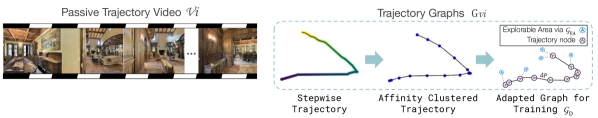
Figure 5: Example from the passive video dataset. Frames of a video trajectory $\mathcal{V}_{i}$ are shown on the left. The stepwise trajectory is then turned into a trajectory graph $G_{\mathcal{V}_{i}}$ via affinity clustering [38] of node image and pose features. $G_{\mathcal{V}_{i}}$ is adapted to train the Global Policy $\mathcal{G}_{D}$ and target direction prediction $\mathcal{G}_{E}A$. An example of an adapted $G_{\mathcal{V}_{i}}$ for training is shown on the left.

5 Experiments

Image-Goal Navigation Task Setup. At the beginning of each episode, the agent is placed in an unseen environment. The agent receives observations from the current state, a 3 x 1 odometry pose reading and RGBD image, and the RGB goal image. Observation and goal images are 120°FOV and of size 480 x 640. An episode is considered a success if the agent is able to reach within $1m$ of the goal location and do so within a maximum episode length of $500$ steps. Each episode is also evaluated by the efficiency of the navigational path from start to goal, which is quantitatively measured by Success weighted by inverse Path Length (SPL) [1]. Note, the narrow field of the agent in this task definition differs from past works which use panoramic views [4]. The decision to use a narrow field is based on our method of training only on passive data. Current passive video datasets of indoor trajectories such as YouTube Tours [24], RealEstate10k [40] and our NRNS passive video dataset, do not contain panoramas.

Action Space. The agent’s action space contains four actions: forward by  .25m, rotate left by  15°, rotate right by  15°, and stop. In our experiments, we consider two cases for pose estimation and action transition. In the first condition the agent has access to ground truth pose and the navigation actions are deterministic. In the second condition, noise is added to the pose estimation and the actuation of the agent. We utilize the realistic pose and actuation noise models from [10], which are similarly used in [4]. The actuation noise adds stochastic rotational and translations transitions to the agent’s navigational actions.

Training Data. Our key contribution is the ability to learn navigation agents from passive data. In theory, our approach can be trained from any passive data source, and we test this in Sec. 5.2 using RealEstate10K [40]. However, since RL-based baselines are trained in the Habitat Simulator [7], we generate our NRNS dataset, of egocentric trajectory videos, using the same Habitat training scenes to provide direct comparison and isolate domain gap issues. Specifically, the trajectory videos are created as follows. A set of 2 - 4 points are randomly selected from the environment using uniform sampling. A video is then generated of the concatenated RGBD frames of the shortest path between consecutive points. Note that the complete video trajectory (from first source to final target) is not step-wise optimal. Frames in the videos are of size 480 X 640 and have a FOV 120°and each frame is associated with a 3 x 1 odometry pose reading. In the noisy setting discussed in Sec. 5, sensor and actuation noise is injected into training trajectories. We create 19K, 43K video trajectories, containing 1, 2.5 million frames respectively, on the Gibson and MP3D datasets. We then use this data to train the NRNS modules, as described in Sec. 4.

Test Environments. We evaluate our approach on the task of image-goal navigation. For testing, we use the Habitat Simulator [7]. We evaluate on the standard test-split for both the Gibson [41] and Matterport3D (MP3D) [42] datasets. For MP3D, we evaluate on 18 environments and for Gibson, we evaluate on 14 environments.

Baselines. We consider a number of baselines to contextualize our Image-Goal Navigation results:

• BC w/ ResNet + GRU. Behavioral Cloning (BC) policy where $I_{t}$ and $I_{G}$ are encoded using a pretrained ResNet-18. Both image encodings and the previous action $a_{t-1}$ are passed through a two layer Gated Recurrent Unit (GRU) with softmax, which outputs the next action $a_{t}$.

• BC w/ ResNet + Metric Map. BC policy: $I_{t}$ and $I_{G}$ are encoded with a ResNet, same as the above policy. This policy keeps a metric map built from the depth images. The metric map is encoded with a linear layer. The metric map encoding and encodings of $I_{t}$ and $I_{G}$ are concatenated and passed into an MLP with softmax, which outputs the next navigational action $a_{t}$.

• End to End RL with DDPPO. An agent is trained end to end with proximal policy optimization [13] in the Habitat Simulator [7] for the image-goal navigation task.

We use and adapt code for baseline algorithms from Chaplot et al. [4]. However, as our setup uses narrow-view cameras instead of panoramas, these adapted baselines perform worse compared to their previously reported performance. This difference in setup also makes direct comparison with [4] infeasible, as they critically rely on panoramic views for localization. The baseline behavioral cloning policies are also trained only using the passive dataset described in Sec. 4. This makes the BC baseline policies directly comparable to the NRNS model.

The end-to-end RL policy is trained using a Habitat implementation of DDPPO [13]. For training we use 8 GPUs and 16 processes per GPU. We first train with 1k episodes per house, which is identical to how NRNS is trained, and we train for 10M steps. To test the scalability of the RL method, we additionally train a model using 5k training episodes per environment (providing the RL agent 5x more data than our NRNS agent) and report the performance of the agent trained on these episodes at 50M steps (5x more compute than NRNS) and 100M steps (10x more compute than NRNS). Training the $\mathcal{G}_{D}$ model takes $\sim$20 epochs, requiring $\sim$8 hours on a single GPU. Training the $\mathcal{G}_{T}$ model takes $\sim$10 epochs, requiring $\sim$4 hours on a single GPU.

Episode Settings. To provide an in-depth understanding of the successes and limitations of our approach, we sub-divide test episodes into two categories: ‘straight’ and ‘curved’. In ‘straight’ episodes, the ratio of shortest path geodesic-distance to euclidean-distance between the start and goal locations is $<1.2$ and rotational difference between the orientation of the start position and goal image is $<45\degree$. All other start-goal location pairs are labeled as ‘curved’ episodes. We make this distinction due to the nature of the narrow field of view of our agent, which strongly affects performance on curved episodes, since the agent must learn to turn both as part of navigating and part of seeking new information about the target location. Also, while a greedy policy being successful on ’straight’ episodes might be expected, a competitive performance on even ’curved’ episodes will highlight how effective our simple model and policy is. We further subdivide each of these 2 categories into 3 sub-categories of difficulty: ‘easy’, ‘medium’ and ‘hard’. Difficulty is determined by the length of the shortest path between the start and goal locations. Following [4], the ‘easy’, ‘medium’ and ‘hard’ settings are $(1.5-3m)$, $(3-5m)$, and $(5-10m)$ respectively. To generate test episodes we uniformly sample the test scene for start-goal location pairs, to create approximately 1000 episodes per setting.

5.1 Results

Tables 1, 2 show the performance of our NRNS model and relevant baselines on the test splits of the Gibson and Matterport datasets. In 6, we visualize an episode of the NRNS agent as it navigates to the goal-image.

NRNS outperforms baselines. Our NRNS algorithm outperforms the BC and end to end RL policies in terms of Success and SPL @ 1m on both datasets. NRNS improves upon the best offline baseline, a Behavioral Cloning (BC) policy with a ResNet and GRU, across splits of Gibson by an absolute 20+% on Straight episodes and 10+% on Curved episodes. We find that a BC policy using a GRU for memory outperforms using only a metric map. We attribute this to a spatial memory (metric map) being less informative for agent exploration than a memory of the visual features and previous steps (GRU). We observe that an end-to-end RL policy trained for 10M steps with 10k epsiodes per house, in simulation performs much weaker than all baselines. With increased data and steps RL baselines unsurprisingly increase in performance, however we find with 5X more data and 10x more compute RL baselines still are outperformed by NRNS. The low performance of behavioral cloning and RL methods for image-goal navigation is unsurprising [4, 15]. This demonstrates the difficulty of learning rewards on low level actions instead of value learning on possible exploration directions, exacerbating the difficulty of exploration in image-goal navigation. Adding to the challenges of the task, all policies must learn the stop action. Previous works [4] have found that adding oracle stopping, to a target-driven RL agent, leads to large gains in performance on image-goal navigation. The limitations of all approaches are seen on the ‘hard’ and ‘curved’ episode settings, showing the overall difficulty of the exploration problem and the challenge of using a narrow field of view.

NRNS is robust to noise. Even with the injection of sensor and actuation noise [10], in both the passive training data and test episodes, NRNS maintains superior or near comparable performance to all baselines. In fact, we find that the addition of noise leads to only an absolute drop in success between .8-8% on Gibson [41] and 1-5% on MP3D [42]. An interesting observation is small increase in performance (w/noise) for the hard-case. We believe this is because gt-distance for hard cases are more error prone and noise during training provides regularization.

Table 1: Comparison of our model (NRNS) with baselines on Image-Goal Navigation on Gibson[41]. We report average Success and Success weighted by inverse Path Length (SPL) @ $1m$. Noise refers to injection of sensor & actuation noise into the train videos and test episodes. ^* denotes using simulator.

				Easy			Medium			Hard
Path Type		Model		Succ $\uparrow$	SPL $\uparrow$		Succ $\uparrow$	SPL $\uparrow$		Succ $\uparrow$	SPL $\uparrow$
Straight		RL (10M steps) * [13]		10.50	6.70		18.10	16.17		11.79	10.85
		RL (extra data + 50M steps)* [13]		36.30	34.93		35.70	33.98		5.94	6.33
		RL (extra data + 100M steps)* [13]		43.20	38.54		36.40	34.89		7.44	7.20
		BC w/ ResNet + Metric Map		24.80	23.94		11.50	11.28		1.36	1.26
		BC w/ ResNet + GRU		34.90	33.43		17.60	17.05		6.08	5.93
		NRNS w/ noise		64.10	55.43		47.90	39.54		25.19	18.09
		NRNS w/out noise		68.00	61.62		49.10	44.56		23.82	18.28
Curved		RL (10M steps)* [13]		7.90	3.27		9.50	7.11		5.50	4.72
		RL (extra data + 50M steps)* [13]		18.10	15.42		16.30	14.46		2.60	2.23
		RL (extra data + 100M steps)* [13]		22.20	16.51		20.70	18.52		4.20	3.71
		BC w/ ResNet + Metric Map		3.10	2.53		0.80	0.71		0.20	0.16
		BC w/ ResNet + GRU		3.60	2.86		1.10	0.91		0.50	0.36
		NRNS w/ noise		27.30	10.55		23.10	10.35		10.50	5.61
		NRNS w/out noise		35.50	18.38		23.90	12.08		12.50	6.84

Table 2: Comparison of our model (NRNS) with baselines on Image-Goal Navigation on MP3D[42].

				Easy			Medium			Hard
Path Type		Model		Succ $\uparrow$	SPL $\uparrow$		Succ $\uparrow$	SPL $\uparrow$		Succ $\uparrow$	SPL $\uparrow$
Straight		RL (10M steps)* [13]		7.50	4.00		3.50	1.73		1.00	0.55
		RL (extra data + 50M steps)* [13]		34.50	30.08		35.70	33.80		10.40	10.07
		RL (extra data + 100M steps)* [13]		36.40	30.84		33.80	31.42		12.00	11.56
		BC w/ ResNet + Metric Map		25.80	24.82		11.30	10.65		3.00	2.93
		BC w/ ResNet + GRU		30.20	29.57		12.70	12.48		4.40	4.34
		NRNS w/ noise		63.80	53.12		36.20	26.92		24.10	16.93
		NRNS w/out noise		64.70	58.23		39.70	32.74		22.30	17.33
Curved		RL (10M steps)* [13]		4.90	1.78		3.20	1.37		1.10	0.46
		RL (extra data + 50M steps)* [13]		15.70	11.34		10.70	9.03		3.90	3.57
		RL (extra data + 100M steps)* [13]		17.90	13.24		15.00	12.17		5.90	4.87
		BC w/ ResNet + Metric Map		4.90	4.23		1.40	1.29		0.40	0.34
		BC w/ ResNet + GRU		3.10	2.61		0.80	0.77		0.10	0.02
		NRNS w/ noise		21.40	8.19		15.40	6.83		10.0	4.86
		NRNS w/out noise		23.70	12.68		16.20	8.34		9.10	5.14

NRNS Module Ablations. Tab. 3 reports detailed ablations of NRNS on the Gibson dataset (see appendix for ablation results on MP3D). We ablate the NRNS approach by testing each module individually. In the ablation experiments, we replace the module output with the ground truth labels or numbers in order to evaluate the affect of each module on the performance of the overall approach. For simplicity, all ablations are trained and tested without sensor or actuation noise. Unsurprisingly, we find that the Global Policy, $\mathcal{G}_{D}$, has a large affect on performance (Row 4 and 8). We find that the largest affects are seen in the ‘hard’ and ‘curved’ test episodes. This is unsurprising because as the distance to the goal increases, the path increases in complexity and the search space of $\mathcal{G}_{D}$ increases.

Table 3: Ablations of NRNS with baselines on Image-Goal Navigation on Gibson [41]. We report average Success and Success weighted by inverse Path Length (SPL) @ $1m$. ✗ denotes a module being replaced by the ground truth labels and a ✓ denotes the NRNS module being used.

		NRNS Ablation				Easy			Medium			Hard
Path Type		$\mathcal{G}_{EA}$	$\mathcal{G}_{T}$	$\mathcal{G}_{D}$		Succ $\uparrow$	SPL $\uparrow$		Succ $\uparrow$	SPL $\uparrow$		Succ $\uparrow$	SPL $\uparrow$
Straight		✗	✗	✗		100.00	99.75		100.00	99.62		100.00	99.57
		✓	✗	✗		99.90	99.05		98.20	95.06		95.91	90.53
		✓	✓	✗		79.40	73.48		71.30	67.48		62.16	58.06
		✓	✓	✓		68.00	61.62		49.10	44.56		23.45	18.84
Curved		✗	✗	✗		100.00	97.62		100.00	97.47		100.00	98.18
		✓	✗	✗		99.70	95.93		97.50	90.14		89.30	79.95
		✓	✓	✗		65.00	56.70		58.10	52.51		47.70	42.28
		✓	✓	✓		35.50	18.38		23.90	12.08		12.50	6.84

5.2 Training on Passive Videos in the Wild

Finally, we demonstrate that our model can be learned from passive videos in the wild. Towards this end, we train our NRNS model using the RealEstate10K dataset [40] which contains YouTube videos of real estate tours. This dataset has 80K clips with poses estimated via SLAM. Note that the average trajectory length is smaller than test time trajectories in Gibson or MP3D, and we therefore only evaluate on ‘easy’ and ‘medium’ settings.  Tab. 4 shows the performance. Note there is a drop in performance compared to training using Gibson videos, which we attribute to domain shift. Even after this drop, our approach, trained on real-world passive videos, outperforms BC baselines and performs competitively against RL baselines. RL baselines have an advantage as they are both trained in the simulator and trained on the Gibson dataset. We believe that the delta between RL and the performance of NRNS trained on RealEstate would close if both were tested on real-world data. We find these results to be a strong indication of the effectiveness of training on passive data.

Table 4: Comparison of our model (NRNS) trained with different sets of passive video data and tested on Image-Goal Navigation on Gibson [41]. We report average Success and Success weighted by inverse Path Length (SPL) @ $1m$. Results shown are tested without sensor & actuation noise.

				Easy			Medium
Path Type	Training Data	Model		Succ $\uparrow$	SPL $\uparrow$		Succ $\uparrow$	SPL $\uparrow$
Straight	RealEstate10k [40]	NRNS		56.42	48.01		30.30	25.67
	MP3D	NRNS		59.80	52.35		37.00	31.89
	Gibson	NRNS		68.00	61.62		49.10	44.56
	Gibson	BC w/ ResNet + GRU		30.20	29.57		12.70	12.48
Curved	RealEstate10k [40]	NRNS		21.10	15.76		12.90	5.57
	MP3D	NRNS		28.26	13.59		11.00	5.10
	Gibson	NRNS		35.50	18.38		23.90	12.08
	Gibson	BC w/ ResNet + GRU		3.10	2.61		0.80	0.77

6 Conclusion

We have presented a simple yet effective approach for learning navigation policies from passive videos. While simulators have become fast, the diversity and scalability of environments still remains a challenge. Our presented approach, NRNS, neither requires access to ground-truth maps nor online policy interaction and hence forgoes the need for a simulator to learn policy functions. We demonstrate that NRNS can outperform RL and behavioral cloning policies by significant margins. We show that NRNS can be trained on passive videos in the wild and still outperform all baselines.

Appendix

7 Implementation Details

Our NRNS model is implemented in PyTorch [43]. We use the each datasets given train/val/test splits. We tune hyperparameters based on val-unseen split performance and use the checkpoint with the highest val-unseen split accuracy to test the NRNS agent on Image-Goal navigation.

7.1 Distance Prediction Network Implementation

$\mathcal{G}_{D}$ is a graph neural network followed by fully connected layers. The fully connected layers take in the pairwise concatenation of the outputted GNN node features and goal image feature. The output of the fully connected layers is the predicted distance to the goal of each node. We implement a graph attention (GAT) network with edge feature attention using the PyTorch Geometric library [44]. The GNN is composed of two GAT layers trained with dropout of .6. For both GAT layers, the input to the layer is node dimension 512, edge dimension 16 and the output dimension of the nodes is 512. The node features output by the second GAT layer are pairwise concatenated with the ResNet18 feature of the goal image. The concatenated features are fed into a 2-layer MLP (512 to 256 to 1) with ReLU activation, and the output is fed through a sigmoid. The network is trained with mean squared error (MSE) loss against the true distance to goal. The network is trained with the Adam optimizer and the learning rate is .0001. Training the $\mathcal{G}_{D}$ model takes 20-25 epochs, requiring $\sim$6 hours on a single GPU.

Unexplored nodes do not have features. Note unexplored nodes do not have features so the features of these nodes are set to zero. Since unexplored nodes do not have children (no outward edges) their empty features are not propagated to any other nodes and only receive propagated features from explored nodes. The graph encoder simply creates the graph adjacency matrix, encodes the explored node as visual 512 features using a ResNet18 via the observed images and sets the edge features to be the transformation matrix between poses of neighboring nodes.

Distance Score Implementation. In $\mathcal{G}_{D}$, the distance label is implemented as a score between 0 to 1 which equals the inverse of the step-wise distance from each node to the goal image calculated by $1-max(distance,30)/30)$. This clipped inverse distance score prioritizes small distances in the loss calculation. During inference time, the distance from the agent’s current location $n_{t}$ to an unexplored node is a added as a ’travel cost’ to the distance prediction. The predicted distance score $d_{i}$ is first converted by to a step-wise distance before the travel cost is added. The $\mathcal{G}_{D}$ network is trained with MSE loss over the predicted and ground truth distance scores. Additionally, loss is only back-propagated over the predictions on unexplored nodes.

7.2 Target Prediction Network Implementation

Input to $\mathcal{G}_{T}$ is the 512 dimension ResNet18 image features for the current and goal images. These features are fed through a single linear layer (512 to 512) followed by a ReLu activation. The hadamard product of the two vectors then fed into a linear layer (512 to 256) followed by a ReLu activation. The output is fed into 3 separate linear layer heads (256 to 1) (the output of these layers are the distance, rotation and switch predictions). The output of the switch linear layer is passed into a sigmoid function. The network is trained using a total loss of the sum of the Smooth l1 loss over the distance and rotation outputs and a Binary Cross Entropy (BCE) loss over the switch predictions. The network is initialized with Xavier uniform and trained with the Adam optimizer, learning rate=.0001 and dropout=.25 after the 2nd linear layer. Training the $\mathcal{G}_{T}$ model takes 10-15 epochs, requiring $\sim$2 hours on a single GPU.

7.3 RL Baseline Implementation

We use the Habitat [7] implementation of DDPPO [13] and follow the standard parameters. We train our DDPO agent on 8 GPUs. During training of the agent receives a terminal reward $r_{T}=2.5\text{SPL}$, and shaped reward $r_{t}(a_{t},s_{t})=-\Delta_{\text{geo-dist}}-0.01$, where $\Delta_{\text{geo-dist}}$ is the change in geodesic distance to the goal by performing action $a_{t}$ in state $s_{t}$. The RL baselines were evaluated over 3 random seeds and the average of the 3 runs was reported.

8 Videos in the Wild

8.1 RealEstate10k Dataset Description

RealEstate10K [40] is a large video dataset of trajectories through mostly indoor scenes. 80k video clips, containing $\sim$10 million frames each corresponding to a provided camera pose. The poses are procured from SLAM and bundle adjustment algorithms run on the videos, and they represent the orientation and path of the camera along the trajectory. The clips are gathered from 10k YouTube videos of real estate footage. The clips are relatively short and range between 1-10 seconds [40]. While the total number of frames in the RealEstate10k clips is large, the total length of the trajectory in meters is on average shorter than the MP3D and Gibson videos. Figure 7 shows the visual difference between frames of the passive video dataset created from the simulator and those taken from YouTube videos.

8.2 Passive Video Transfer Results on MP3D

On the MP3D dataset [42], we perform similar experiments as described in Section 5.2 of the main paper. This section of the main paper only showed results of the experiments on the Gibson dataset [41].

The results of these experiments again demonstrate that NRNS can be learned from passive videos in the wild. We use the same NRNS model trained on RealEstate10K [40] dataset as in Section 5.2 and test on the MP3D test split. Additionally we test an NRNS model trained on passive videos from the Gibson train split, and report performance on MP3D test split.

We find that training on passive videos from the simulator outperforms training on the passive videos on RealEstate10K. This can be attributed a few domain gap factors. RealEstate10K videos are significantly shorter than the simulator generated passive videos, resulting in less training data for the distance prediction network. Additionally, the simulator generated passive videos contain the same actions for the agent’s rotation and translation as in the navigation task, where as RealEstate10K contains a different action space. Despite these domain transfer challenges the NRNS model trained on wild passive videos is able to outperform all other baselines.

Table 5: Comparison of our model (NRNS) trained with different sets of passive video data and tested on Image-Goal Navigation on MP3D [42]. We report average Success and Success weighted by inverse Path Length (SPL) @ $1m$. Results shown are tested without sensor & actuation noise.

				Easy			Medium
Path Type	Training Data	Model		Succ $\uparrow$	SPL $\uparrow$		Succ $\uparrow$	SPL $\uparrow$
Straight	RealEstate10k [40]	NRNS		44.58	39.27		15.81	10.73
	Gibson	NRNS		59.20	54.12		22.90	19.34
	MP3D	NRNS		64.70	58.23		39.70	32.74
	MP3D	BC w/ ResNet + GRU		30.20	29.57		12.70	12.48
Curved	RealEstate10k [40]	NRNS		9.43	4.96		5.30	2.86
	Gibson	NRNS		12.10	5.66		8.48	4.92
	MP3D	NRNS		23.70	12.68		16.20	8.34
	MP3D	BC w/ ResNet + GRU		3.10	2.61		0.80	0.77

9 NRNS Ablation Results on MP3D

We present results of the NRNS ablation experiments on MP3D [42]. The ablation experiments here are identical to those described in Section 5.1, of the main paper, for which performance is shown in Table 3, of the main paper, on Gibson [41]. We observe similar patterns in the NRNS ablations results on MP3D as on Gibson. We again see that the Global Policy $\mathcal{G}_{D}$ has the greatest effect on performance out of all modules particularly on episodes with more difficult settings.

Table 6: Ablations of NRNS with baselines on Image-Goal Navigation on MP3D [42]. We report average Success and Success weighted by inverse Path Length (SPL) @ $1m$. ✗ denotes a module being replaced by the ground truth labels and a ✓ denotes the NRNS module being used.

		NRNS Ablation				Easy			Medium			Hard
Path Type		$\mathcal{G}_{EA}$	$\mathcal{G}_{T}$	$\mathcal{G}_{D}$		Succ $\uparrow$	SPL $\uparrow$		Succ $\uparrow$	SPL $\uparrow$		Succ $\uparrow$	SPL $\uparrow$
Straight		✗	✗	✗		100.00	100.00		99.80	99.07		100.00	99.02
		✓	✗	✗		100.00	100.00		99.00	96.81		96.10	92.65
		✓	✓	✗		74.20	68.19		64.50	60.13		58.40	55.38
		✓	✓	✓		64.70	58.23		39.70	32.74		22.30	17.33
Curved		✗	✗	✗		100.00	94.08		99.90	95.39		100.00	97.00
		✓	✗	✗		100.00	93.06		97.70	90.22		91.60	82.87
		✓	✓	✗		62.20	53.31		54.10	47.51		51.00	44.92
		✓	✓	✓		23.70	12.68		16.20	8.34		9.10	5.14

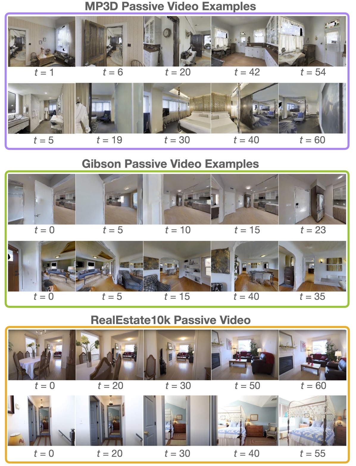
Figure 7: Comparison of the passive videos from different datasets used for training our NRNS agent. MP3D and Gibson passive video frames are images of rendered environments using the habitat simulator and therefore are similar in photo realism. RealEstate10K video frames are taken directly from a real estate tour YouTube video and therefore differ from MP3D and Gibson.

References

- Anderson et al. [2018a] Peter Anderson, Angel Chang, Devendra Singh Chaplot, Alexey Dosovitskiy, Saurabh Gupta, Vladlen Koltun, Jana Kosecka, Jitendra Malik, Roozbeh Mottaghi, Manolis Savva, et al. On evaluation of embodied navigation agents. arXiv preprint arXiv:1807.06757, 2018a.
- Chen et al. [2019a] Tao Chen, Saurabh Gupta, and Abhinav Gupta. Learning exploration policies for navigation. International Conference on Learning Representations, 2019a.
- Ramakrishnan et al. [2020] Santhosh K Ramakrishnan, Ziad Al-Halah, and Kristen Grauman. Occupancy anticipation for efficient exploration and navigation. In European Conference on Computer Vision, 2020.
- Chaplot et al. [2020a] Devendra Singh Chaplot, Ruslan Salakhutdinov, Abhinav Gupta, and Saurabh Gupta. Neural topological slam for visual navigation. In Computer Vision and Pattern Recognition, 2020a.
- Batra et al. [2020] Dhruv Batra, Aaron Gokaslan, Aniruddha Kembhavi, Oleksandr Maksymets, Roozbeh Mottaghi, Manolis Savva, Alexander Toshev, and Erik Wijmans. ObjectNav Revisited: On Evaluation of Embodied Agents Navigating to Objects. In arXiv:2006.13171, 2020.
- Chaplot et al. [2020b] Devendra Singh Chaplot, Dhiraj Prakashchand Gandhi, Abhinav Gupta, and Russ R Salakhutdinov. Object goal navigation using goal-oriented semantic exploration. Neural Information Processing Systems, 2020b.
- Savva et al. [2019] Manolis Savva, Abhishek Kadian, Oleksandr Maksymets, Yili Zhao, Erik Wijmans, Bhavana Jain, Julian Straub, Jia Liu, Vladlen Koltun, Jitendra Malik, et al. Habitat: A platform for embodied ai research. In International Conference on Computer Vision, 2019.
- Anderson et al. [2018b] Peter Anderson, Qi Wu, Damien Teney, Jake Bruce, Mark Johnson, Niko Sünderhauf, Ian Reid, Stephen Gould, and Anton van den Hengel. Vision-and-Language Navigation: Interpreting visually-grounded navigation instructions in real environments. In Computer Vision and Pattern Recognition, 2018b.
- Kolve et al. [2017] Eric Kolve, Roozbeh Mottaghi, Winson Han, Eli VanderBilt, Luca Weihs, Alvaro Herrasti, Daniel Gordon, Yuke Zhu, Abhinav Gupta, and Ali Farhadi. AI2-THOR: An Interactive 3D Environment for Visual AI. Computer Vision and Pattern Recognition, 2017.
- Chaplot et al. [2020c] Devendra Singh Chaplot, Dhiraj Gandhi, Saurabh Gupta, Abhinav Gupta, and Ruslan Salakhutdinov. Learning to explore using active neural slam. In International Conference on Learning Representations, 2020c.
- Zhu et al. [2017] Yuke Zhu, Roozbeh Mottaghi, Eric Kolve, Joseph J Lim, Abhinav Gupta, Li Fei-Fei, and Ali Farhadi. Target-driven visual navigation in indoor scenes using deep reinforcement learning. In International Conference on Robotics and Automation, 2017.
- Gupta et al. [2017] Saurabh Gupta, James Davidson, Sergey Levine, Rahul Sukthankar, and Jitendra Malik. Cognitive mapping and planning for visual navigation. In Computer Vision and Pattern Recognition, 2017.
- Wijmans et al. [2020] Erik Wijmans, Abhishek Kadian, Ari Morcos, Stefan Lee, Irfan Essa, Devi Parikh, Manolis Savva, and Dhruv Batra. Dd-ppo: Learning near-perfect pointgoal navigators from 2.5 billion frames. In International Conference on Learning Representations, 2020.
- Wu et al. [2019] Yi Wu, Yuxin Wu, Aviv Tamar, Stuart Russell, Georgia Gkioxari, and Yuandong Tian. Bayesian relational memory for semantic visual navigation. In International Conference on Computer Vision, 2019.
- Mezghani et al. [2021] Lina Mezghani, Sainbayar Sukhbaatar, Thibaut Lavril, Oleksandr Maksymets, Dhruv Batra, Piotr Bojanowski, and Karteek Alahari. Memory-augmented reinforcement learning for image-goal navigation. arXiv preprint arXiv:2101.05181, 2021.
- Yang et al. [2018] Wei Yang, Xiaolong Wang, Ali Farhadi, Abhinav Gupta, and Roozbeh Mottaghi. Visual semantic navigation using scene priors. International Conference on Learning Representations, 2018.
- Eysenbach et al. [2019] Benjamin Eysenbach, Ruslan Salakhutdinov, and Sergey Levine. Search on the replay buffer: Bridging planning and reinforcement learning. In Neural Information Processing Systems, 2019.
- Savinov et al. [2018] Nikolay Savinov, Alexey Dosovitskiy, and Vladlen Koltun. Semi-parametric topological memory for navigation. In International Conference on Learning Representations, 2018.
- Mirowski et al. [2018] Piotr Mirowski, Matthew Koichi Grimes, Mateusz Malinowski, Karl Moritz Hermann, Keith Anderson, Denis Teplyashin, Karen Simonyan, Koray Kavukcuoglu, Andrew Zisserman, and Raia Hadsell. Learning to navigate in cities without a map. In Neural Information Processing Systems, 2018.
- Emmons et al. [2020] Scott Emmons, Ajay Jain, Michael Laskin, Thanard Kurutach, Pieter Abbeel, and Deepak Pathak. Sparse graphical memory for robust planning. In Neural Information Processing Systems, 2020.
- Chen et al. [2019b] Kevin Chen, Juan Pablo de Vicente, Gabriel Sepulveda, Fei Xia, Alvaro Soto, Marynel Vázquez, and Silvio Savarese. A behavioral approach to visual navigation with graph localization networks. In Robotics: Science and Systems, 2019b.
- Shah et al. [2020] Dhruv Shah, Benjamin Eysenbach, Gregory Kahn, Nicholas Rhinehart, and Sergey Levine. Ving: Learning open-world navigation with visual goals. International Conference on Robotics and Automation, 2020.
- Brahmbhatt and Hays [2017] Samarth Brahmbhatt and James Hays. Deepnav: Learning to navigate large cities. In Proceedings of the IEEE conference on computer vision and pattern recognition, 2017.
- Chang et al. [2020] Matthew Chang, Arjun Gupta, and Saurabh Gupta. Semantic visual navigation by watching youtube videos. In Neural Information Processing Systems, 2020.
- Ravichandar et al. [2020] Harish Ravichandar, Athanasios S Polydoros, Sonia Chernova, and Aude Billard. Recent advances in robot learning from demonstration. Annual Review of Control, Robotics, and Autonomous Systems, 2020.
- Silver et al. [2012] David Silver, J Andrew Bagnell, and Anthony Stentz. Active learning from demonstration for robust autonomous navigation. In International Conference on Robotics and Automation, 2012.
- Pan et al. [2020] Xinlei Pan, Tingnan Zhang, Brian Ichter, Aleksandra Faust, Jie Tan, and Sehoon Ha. Zero-shot imitation learning from demonstrations for legged robot visual navigation. In International Conference on Robotics and Automation, 2020.
- Siegel et al. [2020] Noah Y Siegel, Jost Tobias Springenberg, Felix Berkenkamp, Abbas Abdolmaleki, Michael Neunert, Thomas Lampe, Roland Hafner, Nicolas Heess, and Martin Riedmiller. Keep doing what worked: Behavioral modelling priors for offline reinforcement learning. arXiv preprint arXiv:2002.08396, 2020.
- Levine et al. [2020] Sergey Levine, Aviral Kumar, George Tucker, and Justin Fu. Offline reinforcement learning: Tutorial, review, and perspectives on open problems. arXiv preprint arXiv:2005.01643, 2020.
- Kumar et al. [2020] Aviral Kumar, Aurick Zhou, George Tucker, and Sergey Levine. Conservative q-learning for offline reinforcement learning. arXiv preprint arXiv:2006.04779, 2020.
- Beeching et al. [2020] Edward Beeching, Jilles Dibangoye, Olivier Simonin, and Christian Wolf. Learning to plan with uncertain topological maps. In European Conference on Computer Vision, 2020.
- Epstein et al. [2017] Russell A Epstein, Eva Zita Patai, Joshua B Julian, and Hugo J Spiers. The cognitive map in humans: spatial navigation and beyond. Nature Neuroscience, 2017.
- Tolman [1948] Edward C Tolman. Cognitive maps in rats and men. Psychological Review, 1948.
- Foo et al. [2005] Patrick Foo, William H Warren, Andrew Duchon, and Michael J Tarr. Do humans integrate routes into a cognitive map? map-versus landmark-based navigation of novel shortcuts. Journal of Experimental Psychology: Learning, Memory, and Cognition, 2005.
- Wang and Spelke [2002] Ranxiao Frances Wang and Elizabeth S Spelke. Human spatial representation: Insights from animals. Trends in Cognitive Sciences, 2002.
- Veličković et al. [2017] Petar Veličković, Guillem Cucurull, Arantxa Casanova, Adriana Romero, Pietro Liò, and Yoshua Bengio. Graph attention networks. International Conference on Learning Representations, 2017.
- He et al. [2016] Kaiming He, Xiangyu Zhang, Shaoqing Ren, and Jian Sun. Deep residual learning for image recognition. In Computer Vision and Pattern Recognition, 2016.
- Frey and Dueck [2007] Brendan J Frey and Delbert Dueck. Clustering by passing messages between data points. Science, 2007.
- Zhou et al. [2017] Bolei Zhou, Agata Lapedriza, Aditya Khosla, Aude Oliva, and Antonio Torralba. Places: A 10 million image database for scene recognition. Transactions on Pattern Analysis and Machine Intelligence, 2017.
- Zhou et al. [2018] Tinghui Zhou, Richard Tucker, John Flynn, Graham Fyffe, and Noah Snavely. Stereo magnification: Learning view synthesis using multiplane images. In SIGGRAPH, 2018.
- Xia et al. [2018] Fei Xia, Amir R Zamir, Zhiyang He, Alexander Sax, Jitendra Malik, and Silvio Savarese. Gibson env: Real-world perception for embodied agents. In Computer Vision and Pattern Recognition, 2018.
- Chang et al. [2017] Angel Chang, Angela Dai, Thomas Funkhouser, Maciej Halber, Matthias Niessner, Manolis Savva, Shuran Song, Andy Zeng, and Yinda Zhang. Matterport3d: Learning from rgb-d data in indoor environment. International Conference on 3D Vision, 2017.
- Paszke et al. [2019] Adam Paszke, Sam Gross, Francisco Massa, Adam Lerer, James Bradbury, Gregory Chanan, Trevor Killeen, Zeming Lin, Natalia Gimelshein, Luca Antiga, et al. Pytorch: An imperative style, high-performance deep learning library. In Neural Information Processing Systems, 2019.
- Fey and Lenssen [2019] Matthias Fey and Jan E. Lenssen. Fast graph representation learning with PyTorch Geometric. In International Conference on Learning Representations, 2019.