An elementary proof of phase transition
in the planar XY model

Abstract.

Using elementary methods we obtain a power-law lower bound on the two-point function of the planar XY spin model at low temperatures. This was famously first rigorously obtained by Fröhlich and Spencer [FroSpe] and establishes a Berezinskii–Kosterlitz–Thouless phase transition in the model. Our argument relies on a new loop representation of spin correlations, a recent result of Lammers [Lammers] on delocalisation of general integer-valued height functions, and classical correlation inequalities.

1. Introduction and main result

Let $G=(V,E)$ be a finite graph. Given a collection of nonnegative coupling constants $J=(J_{e})_{e\in E}$, and an inverse temperature $\beta>0$, the XY model (with free boundary conditions) is a random spin configuration $\sigma\in\mathbb{S}^{V}$, where $\mathbb{S}=\{z\in\mathbb{C}:|z|=1\}$ is the complex unit circle, sampled according to the Gibbs distribution

$$d\mu_{G,\beta}(\sigma)\propto\exp\Big{(}\tfrac{1}{2}\beta\sum_{vv^{\prime}\in E}J_{vv^{\prime}}(\sigma_{v}\bar{\sigma}_{v^{\prime}}+\bar{\sigma}_{v}\sigma_{v^{\prime}})\Big{)}\prod_{v\in V}d\sigma_{v},$$ (1)

where $vv^{\prime}$ denotes the edge $\{v,v^{\prime}\}$, and $d\sigma_{v}$ is the uniform probability measure on $\mathbb{S}$. For simplicity of notation, unless stated otherwise, we will assume that $J_{e}=1$ for all $e$. However, our results extend naturally to nonhomogeneous coupling constants. We will write $\langle\cdot\rangle_{G,\beta}$ for the expectation with respect to $\mu_{G,\beta}$. The observable of main interest for us will be the two-point function $\langle\sigma_{a}\bar{\sigma}_{b}\rangle_{G,\beta}$, $a,b\in V$, and its infinite volume limit

$$\langle\sigma_{a}\bar{\sigma}_{b}\rangle_{\Gamma,\beta}=\lim_{G\nearrow\Gamma}\langle\sigma_{a}\bar{\sigma}_{b}\rangle_{G,\beta},$$

where $\Gamma$ is an infinite planar lattice.

Note that if $\sigma_{v}=e^{i\theta_{v}}$, $\theta_{v}\in(-\pi,\pi]$, then $\sigma_{v}\bar{\sigma}_{v^{\prime}}+\bar{\sigma}_{v}\sigma_{v^{\prime}}=2\cos(\theta_{v}-\theta_{v^{\prime}})$. This means that the model is ferromagnetic, i.e., pairs of neighbouring spins that are (almost) aligned have smaller energy and hence are statistically favoured. A natural question is wether varying $\beta$ leads to a ferromagnetic order–disorder phase transition in the model. The classical theorem of Mermin and Wagner [MerWag] excludes this possibility when the underlying lattice $\Gamma$ is two-dimensional. Moreover, McBryan and Spencer showed that at any finite temperature $\langle\sigma_{a}\bar{\sigma}_{b}\rangle_{\mathbb{Z}^{2},\beta}$ decays to zero at least as fast as a power of the distance between $a$ and $b$. On the other hand, it is known by the work of Fröhlich, Simon and Spencer [FSS] that in higher dimensions the model exhibits long-range order at low temperatures and the two-point function does not decay to zero.

Even though there is no spontaneous symmetry breaking, Berezinskii [Ber1, Ber2], and Kosterlitz and Thouless [KosTho] predicted that a different type of phase transition takes place in two dimensions. It should be understood in terms of interacting topological excitations of the model, the so called vortices and antivortices. They are those faces of the graph where the XY configuration makes a full clockwise or anticlockwise turn respectively when one traverses the edges of the face in a clockwise manner. Vortices and antivortices interact through a Coulomb interaction, and are energetically favoured to form short-distance pairs of vortex-antivortex. However, such configurations have clearly much smaller entropy. The Berezinskii–Kosterlitz–Thouless (BKT) phase transition happens when, while increasing the temperature, entropy wins agains energy, and the vortex-antivortex pairs unbind and form a plasma of freely spaced vortices and antivortices. This regime corresponds to exponential decay, whereas the phase with bound vortex-antivortex pairs should exhibit power-law decay of the two-point function. A rigorous lower bound of this type for low temperatures, and therefore a proof of the BKT phase transition was first obtained in the celebrated work of Fröhlich and Spencer [FroSpe] who also derived analogous results for the Villain spin model. Their proof uses a multi-scale analysis of the Coulomb gas, and the main purpose of the present article is to present an alternative and less technically involved argument for the existence of phase transition in two dimensions.

To be more precise, we introduce a new loop representation for the two-point function in the XY model that can be used to transfer probabilistic information from the dual integer-valued height function model to the XY model. Along the way we also show that the height function possesses the crucial absolute-value-FKG property. This, together with a recent elementary delocalisation result for general height functions obtained by Lammers [Lammers], is used to prove existence of the BKT phase transition.

Theorem 1 (Berezinskii–Kosterlitz–Thouless phase transition).

There exists $\beta_{c}\in(0,\infty)$ such that

1. for all $\beta<\beta_{c}$, there exists $c=c(\beta)>0$ such that for all $v,v^{\prime}\in\mathbb{Z}^{2}$,

   $$\langle\sigma_{v}\overline{\sigma}_{v^{\prime}}\rangle_{\mathbb{Z}^{2},\beta}\leq e^{-c|v-v^{\prime}|},$$

2. for all $\beta\geq\beta_{c}$ and all distinct $v,v^{\prime}\in\mathbb{Z}^{2}$,

   $$\langle\sigma_{v}\overline{\sigma}_{v^{\prime}}\rangle_{\mathbb{Z}^{2},\beta}\geq\frac{1}{8|v-v^{\prime}|}.$$

We note that unlike in the original proof of Fröhlich and Spencer, we do not show that the rate of decay approaches zero when so does the temperature. However, we establish a type of sharpness which says that there is no other behaviour than exponential and power-law decay. The short proof of sharpness is independent of the rest of the argument. In the first step we classically use the Lieb–Rivasseau inequality [Lieb, Riv] to establish a sharp transition between exponential decay and nonsummability of correlations (similarly to the proof for the Ising model [DCT]). To conclude a uniform power-law lower bound as in $(ii)$ whenever the correlations are not summable we use the Messager–Miracle-Sole inequality [MMS] on monotonicity of correlations with respect to the position of the vertex on the lattice.

We also note that our proof works (with minor modifications and a different, implicit multiplicative constant in $(ii)$) for other infinite graphs that in addition to being translation invariant possess reflection and rotation symmetries.

For a more detailed overview of the XY model, we refer the reader to [PelSpi, FriVel], and for expositions of the argument of Fröhlich and Spencer, we refer to [KP, GS].

This article is organised as follows.

• In Section 2 we introduce the dual of the planar XY model in form of an integer-valued height function defined on the faces of the graph. We also establish positive association of its absolute value (the absolute-value-FKG property), and recall the delocalisation result of Lammers [Lammers].

• In Section 3 we define a random collection of loops on the graph that carries probabilistic information about both the XY spins and the dual height function. Although this is a well known object that goes back to the works of Symanzik [Sym], and Brydges, Fröhlich and Spencer [BFS], the formula that relates the two-point function to the probability of two points being connected by a loop (Lemma 8) is new and crucial to our argument.

• In Section 4 we give an elementary argument which states that if the height function delocalises at some temperature, then the spin two-point function does not decay exponentially.

• In Section 5 we use the above ingredients to show that on any translation invariant graph, there exists a finite temperature at which the two-point function does not decay exponentially. This is not immediate as the result of Lammers [Lammers] applies only to trivalent graphs. However, a simple graph-modification argument together with the Ginibre inequality allows to change the setup from a general graph to a triangulation (a graph whose dual is trivalent).

• In Section 6 we finish the proof of the main theorem. We use the Lieb–Rivasseau inequality [Lieb, Riv] and the inequality of Lemma 19 to show that the absence of exponential decay implies a power-law lower bound on the two-point function. The proof of sharpness relies only on this section and Lemma 19.

• Finally, independently of the rest of the article, in Appendix A we develop a new loop representation for squares and products of spin correlation functions in the XY model. As an application we present new correlation inequalities and give new combinatorial proofs of the Lieb–Rivasseau [Lieb, Riv], and the Messager–Miracle-Sole inequality [MMS]. We hope this representation will be useful in the further study of the XY model.

Acknowledgements

ML is grateful to Roland Bauerschmidt and Hugo Duminil-Copin for inspiring discussions on the XY model. We also thank Christophe Garban for useful remarks on a draft.

2. The dual height function

To define the dual model we assume that $G$ is planar and we need to introduce currents. To this end, let $\vec{E}$ be the set of directed edges of $G$, and let $\mathbb{N}=\{0,1,\ldots\}$. A function $\mathbf{n}:\vec{E}\to\mathbb{N}$ is called a current on $G$. For a current $\mathbf{n}$, we define $\delta\mathbf{n}:V\to\mathbb{Z}$ by

$$\delta\mathbf{n}_{v}=\sum_{v^{\prime}\sim v}\mathbf{n}_{(v,v^{\prime})}-\mathbf{n}_{(v^{\prime},v)}.$$

Hence if $\delta\mathbf{n}_{v}$ is positive, then the amount of outgoing current is larger than the incoming current, an we think of $v$ as a source. Likewise if $\delta\mathbf{n}_{v}$ is negative, there is more incoming current and $v$ is a sink. A current is sourceless if $\delta\mathbf{n}_{v}=0$ for all $v\in V$.

We define $\Omega_{0}$ to be the set of all (sourceless) currents. Sourceless currents naturally define a height function $h$ on the set of faces of $G$, denoted by $U$, where the height of the outer face is set to zero, and the increment of the height between two faces $u$ and $u^{\prime}$ is equal to

$$h(u)-h(u^{\prime})=\mathbf{n}_{(v,v^{\prime})}-\mathbf{n}_{(v^{\prime},v)},$$

where the primal directed edge $(v,v^{\prime})$ crosses the dual directed edge $(u,u^{\prime})$ from right to left. That this yields a well defined function on the faces of $G$ follows from the fact that $\delta\mathbf{n}=0$. We define the XY weight of a current by

$$w_{\beta}(\mathbf{n})=\prod_{(v,v^{\prime})\in\vec{E}}\frac{1}{\mathbf{n}_{(v,v^{\prime})}!}\Big{(}\frac{\beta J_{vv^{\prime}}}{2}\Big{)}^{\mathbf{n}_{(v,v^{\prime})}},$$ (2)

These weights appear naturally in the expansion of the partition function of the XY model into a sum over sourceless currents after one expands the exponentials in (1) into a power series in the variables $\tfrac{1}{2}\beta J_{vv^{\prime}}\sigma_{v}\bar{\sigma}_{v^{\prime}}$ for each directed edge $(v,v^{\prime})\in\vec{E}$, and then integrates out the $\sigma$ variables. They will also appear in the analogous classical expansion for spin correlations (11).

We note that using currents to define a model on the dual graph is an instance of planar duality of abelian spin systems [dubedat2011topics], and the fact that the function is integer valued is a consequence of $\mathbb{Z}$ being the dual group of the unit circle.

Clearly, the weight (2) defines a probability measure $\mathbb{P}_{G,\beta}$ on currents and hence also on height functions. In terms of the height function it is a Gibbs measure given by

$$\mathbb{P}_{G,\beta}(h)\propto\exp\Big{(}-\sum_{uu^{\prime}\in E^{\dagger}}\mathcal{V}_{e}^{\beta}(h(u)-h(u^{\prime}))\Big{)},$$ (3)

where $E^{\dagger}$ is the set of dual edges of $G$, and where the symmetric potentials $\mathcal{V}^{\beta}_{e}:\mathbb{Z}\to\mathbb{R}$ are given by

$$\mathcal{V}^{\beta}_{e}(k)=-\log\Big{(}\sum_{i=0}^{\infty}\frac{1}{i!(i+|k|)!}\Big{(}\frac{\beta J_{e}}{2}\Big{)}^{2i+|k|}\Big{)}=-\log I_{k}({\beta J_{e}})$$ (4)

with $I_{k}$ being the modified Bessel function. We again note that we will usually set all $J_{e}=1$ to simplify the notation.

A well known Turán-type inequality for modified Bessel functions [Bessel] states that for any $k\geq 0$ and $\beta>0$,

$$I_{k}^{2}(\beta)\geq I_{k-1}(\beta)I_{k+1}(\beta)$$ (5)

which means that $\mathcal{V}^{\beta}_{e}$ is convex on the integers. This puts the model in the well studied framework of height functions with a convex potential (see e.g. [sheffield]).

2.1. Gibbs measures and delocalisation

To state the delocalisation result of Lammers we will need the notion of a Gibbs measure for height functions on infinite graphs (though we will not directly work with it in the remainder of the article). Let $\Gamma=(V,E)$ be an infinite planar graph and $\Gamma^{\dagger}=(U,E^{\dagger})$ its planar dual. If $\nu$ is a measure on height functions $\varphi:\mathbb{Z}^{U}\to\mathbb{Z}$ and $\Lambda\subset U$ a finite subset, write $\nu_{\Lambda}$ for the measure restricted to $\Lambda$. Let $\mathcal{V}=(\mathcal{V}_{e})_{e\in E\dagger}$ be a family of convex symmetric potentials. We call $\nu$ a Gibbs measure for the potential $\mathcal{V}$ if for every such $\Lambda$, it satisfies the Dobrushin–Lanford–Ruelle relation

$$\nu_{\Lambda}(\cdot)=\int_{\mathbb{Z}^{U}}\nu^{\varphi}_{\Lambda}(\cdot)d\nu(\varphi),$$

where $\nu^{\varphi}_{\Lambda}$ is the Gibbs measure on height functions $h\in\mathbb{Z}^{U}$ given as in (3) (but with $\mathcal{V}^{\beta}$ replaced by $\mathcal{V}$) and conditioned on $h$ being equal to $\varphi$ on the boundary of $\Lambda$.

In what follows we will always assume that $\Gamma$ is locally finite and invariant under the action of a $\mathbb{Z}^{2}$-isomorphic lattice. We say that $\nu$ is translation invariant if it is invariant under the same acton.

In a recent beautiful work [Lammers] Lammers gave a condition on the potential that guarantees that there are no translation invariant Gibbs measures on graphs of degree three (trivalent graphs).

Theorem 2 (Lammers [Lammers]).

Let $\Gamma^{\dagger}=(U,E^{\dagger})$ be as above and moreover trivalent. If for every $e\in E^{\dagger}$,

$$\mathcal{V}_{e}(\pm 1)\leq\mathcal{V}_{e}(0)+\log(2),$$ (6)

then there are no translation invariant Gibbs measures for $\mathcal{V}$.

This together with the dichotomy stated in Theorem 3 will be one of the key ingredients of the proof of the main theorem.

2.2. Absolute-value-FKG and dichotomy

In this section, we prove that the height function satisfies the absolute-value-FKG property, which is known to imply the following dichotomy.

Let $\Gamma=(V,E)$ be a translation invariant graph, and let $0$ be a chosen face of $\Gamma$. Define $B_{n}$ to be the subgraph of $\Gamma$ induced by the vertices in $V$ that lie on at least one face of $\Gamma$ that is contained in the graph ball of radius $n$ on $\Gamma^{\dagger}$. We introduce this slightly convoluted definition to guarantee the following three properties: $0$ belongs to all $B_{n}$, also $B_{n}\nearrow\Gamma$ as $n\to\infty$, and finally, the weak dual graph of $B_{n}$ (the dual graph with the vertex corresponding to the external face of $B_{n}$ removed) is a subgraph of $\Gamma^{\dagger}$.

Theorem 3.

Consider the setup as above. Then for every $\beta>0$, exactly one of the following two occurs:

1. (localisation) There exists a $C<\infty$ such that uniformly over all $n$,

   $$\mathbb{E}_{B_{n},\beta}[|h(0)|]\leq C.$$

2. (delocalisation) There are no translation invariant Gibbs measures for the potential (4).

Proof.

This is a consequence of the absolute-value-FKG property proved below (Proposition 4) and standard arguments using monotonicity in boundary conditions. See for example [CPST, Lemma 2.2] or [LamOtt, Theorem 2.7]. ∎

The remainder of this section is devoted to proving the following version of the absolute-value-FKG property.

Proposition 4.

Let $G=(V,E)$ be a finite graph and $U$ the set of its faces. Then for all $\beta>0$, and all $\Psi,\Phi:\mathbb{N}^{U}\to\mathbb{R}_{+}$ increasing functions,

$$\mathbb{E}_{G,\beta}[\Psi(|h|)\Phi(|h|)]\geq\mathbb{E}_{G,\beta}[\Psi(|h|)]\mathbb{E}_{G,\beta}[\Phi(|h|)].$$

The proposition is easiest to prove for small $\beta$. We extend this to general $\beta$ afterwards.

Lemma 5.

The above holds true for all $\beta\leq 1$.

Proof.

We rely on a result of Lammers and Ott [LamOtt, Theorem 2.8], stating that if

$$\mathcal{V}_{e}^{\beta}(k-1)-2\mathcal{V}_{e}^{\beta}(k)+\mathcal{V}_{e}^{\beta}(k+1)=-\log\Big{(}\frac{I_{k-1}(\beta)I_{k+1}(\beta)}{I_{k}(\beta)^{2}}\Big{)}$$

is a nonincreasing function of $k$ on $\{0,1,\ldots\}$, then $\mathbb{P}_{G,\beta}$ is absolute-value-FKG. We define $r_{k}=\tfrac{1}{\beta}\frac{I_{k}(\beta)}{I_{k-1}(\beta)}$, and need to show that $r_{k}^{2}\leq r_{k-1}r_{k+1}$ for all $k\geq 0$. The well known recurrence relation

$$I_{k-1}(\beta)=\tfrac{2k}{\beta}I_{k}(\beta)+I_{k+1}(\beta)\qquad\text{yields}\qquad r_{k}=(2k+\beta^{2}r_{k+1})^{-1}.$$

Hence it is enough to prove that

$$(2k+\epsilon_{k+1})(2(k+2)+\epsilon_{k+3})\leq(2(k+1)+\epsilon_{k+2})^{2},$$

where $\epsilon_{k}=\beta^{2}r_{k}$. Using the Turán inequality (5), it follows that $0\leq r_{k+1}\leq r_{k}$, and therefore it is sufficient to establish that

$$R_{k}:=(2k+\epsilon_{k+1})(2k+4+\epsilon_{k+1})-(2k+2)^{2}=4(k+1)\epsilon_{k+1}+\epsilon_{k+1}^{2}-4\leq 0.$$

At the same time, simply using the definition of $r_{k+1}$ and comparing the Taylor expansions (4) of $I_{k+1}$ and $I_{k}$ term by term gives $\epsilon_{k+1}\leq\beta^{2}/(2k+2)$. Therefore, when $\beta\leq 1$, we have $R_{k}\leq\epsilon_{k+1}^{2}-2\leq 0$ for all $k\geq 0$, which concludes the proof. ∎

To treat general values of $\beta$, we will use a trick which consists in replacing each edge of $G$ by $s=\lceil\beta\rceil$ consecutive edges, and reducing the parameter $\beta$ by the factor $s$, together with the following convolution property of the modified Bessel functions.

Lemma 6.

For all $k,l\in\mathbb{Z}$ and all $\beta,\beta^{\prime}\geq 0$,

$$\sum_{m\in\mathbb{Z}}I_{k-m}(\beta)I_{m-l}(\beta^{\prime})=I_{k-l}(\beta+\beta^{\prime}).$$

Proof.

This is a classical identity which follows from the fact that $I_{k}(\beta)/e^{\beta}=\mathbb{P}(Z-Z^{\prime}=k)$, where $Z,Z^{\prime}$ are independent Poisson random variables with mean $\beta/2$, and the fact that a sum of independent Poisson random variables is Poisson. ∎

With this we can prove Proposition 4.

Proof of Proposition 4.

Let $G_{s}=(V_{s},E_{s})$ be $G$ with each edge replaced by $s$ consecutive edges, and let $h_{s}$ be the height function on $G_{s}$ with law $\mu_{G_{s},\beta/s}$. By Lemma 6 (and an induction argument) the restriction of $h_{s}$ to $V$ has the same law as $h_{1}$. Moreover, $\beta/s\leq 1$ by definition of $s$, which by Lemma 5 implies that $\mu_{s}$ is absolute-value-FKG. To finish the proof it is enough to notice that any increasing function on $\mathbb{N}^{V}$ is also increasing on $\mathbb{N}^{V_{s}}$. ∎

Remark 1.

An interesting consequence of the idea above (that we will not use in this article) is the following. Consider the case when $s$ from above is independent of $\beta$ and diverges to infinity. In this limit, the height function becomes well defined at every point of every dual edge. Here we think of the dual graph as the so called cable graph, i.e., every dual edge $e$ is identified with a continuum interval of length $J_{e}\beta$. Then the distribution of the height on an edge, when conditioned on the values at the endpoints, is one of the difference of two Poisson processes with intensity $J_{e}\beta/2$ each, and conditioned on the value at the endpoints. One can check that the model exhibits a spatial Markov property on the full cable graph and not only on the vertices. This is in direct analogy with the cable graph representation of the discrete Gaussian free field, where the vertex-field can be extended to the edges via Brownian bridges (see e.g. [Lupu] and the references therein).

3. Loop representation of currents and path reversal

The purpose of this section is mainly to develop a loop representation for the two-point function of the XY model. The important aspect of our approach is that the correlations are represented as probabilities for loop connectivities in random ensembles of closed loops. This is in contrast with most of the classical representations that write correlation functions as ratios of partition functions of loops, where in the numerator, in addition to loops, one also sums over open paths between the points of insertion in the correlator [Sym, BFS]. We note that a similar idea to ours appears in the work of Benassi and Ueltschi [BenUel], but due to technical differences in the framework (see Remark 4), the formula for the two-point function obtained in [BenUel] is not as transparent as ours.

Let $G=(V,E)$ be a finite, not necessarily planar graph. We say that a multigraph $\mathcal{M}$ on $V$ is a submultigraph of $G$ if after identifying the multiple copies of the same edge in $\mathcal{M}$ it is a subgraph of $G$.

Definition (Loop configurations outside $S$).

Let $\mathcal{M}$ be a submultigraph of $G$, and let $S\subseteq V$. A loop configuration (on $\mathcal{M}$) outside $S$ is a collection of

• unrooted directed loops on $\mathcal{M}$ avoiding $S$, and

• directed open paths on $\mathcal{M}$ starting and ending in $S$ (and not visiting $S$ except at their start and end vertex),

such that every edge of $\mathcal{M}$ is traversed exactly once by a loop or a path.

We write ${\mathcal{L}}^{S}$ for the set of all loop configurations outside $S$, and define a weight for $\omega\in{\mathcal{L}}^{S}$ by

$$\lambda^{S}_{\beta}(\omega)=\prod_{v\in V\setminus S}\frac{1}{(\deg_{\mathcal{M}}(v)/2)!}\prod_{e\in E}\frac{1}{\mathcal{M}_{e}!}\Big{(}\frac{\beta}{2}\Big{)}^{\mathcal{M}_{e}},$$ (7)

where $\mathcal{M}$ is the underlying multigraph, and $\mathcal{M}_{e}$ is the number of copies of $e$ in $\mathcal{M}$. When $S=\emptyset$, a configuration is composed only of loops that can visit every vertex in $V$, and we simply call it a loop configuration.

An important feature of the weight (7) is that it depends on $\omega$ only through $\mathcal{M}$. Also note, that if $S^{\prime}\subseteq S$, then there is a natural map $\rho:\mathcal{L}^{S^{\prime}}\to\mathcal{L}^{S}$ that consists in forgetting (or cutting) the loop connections at the vertices in $S\setminus S^{\prime}$. Under this map, each configuration in $\mathcal{L}^{S}$ has $\prod_{v\in S\setminus S^{\prime}}{(\deg_{\mathcal{M}}(v)/2)!}$ preimages, each of them having the same weight, and hence

$$\sum_{\tilde{\omega}\in\rho^{-1}[\omega]}\lambda^{S^{\prime}}_{\beta}(\tilde{\omega})=\lambda^{S}_{\beta}(\omega).$$ (8)

This consistency property will be useful later on.

For now, let $|\mathbf{n}|:E\to\mathbb{N}$ be the amplitude of a current $\mathbf{n}$, i.e.

$$|\mathbf{n}|_{vv^{\prime}}:=\mathbf{n}_{(v,v^{\prime})}+\mathbf{n}_{(v^{\prime},v)}.$$

Definition (Multigraph of a current and consistent configurations).

For a current $\mathbf{n}$, let $\mathcal{M}_{\mathbf{n}}$ be the submultigraph of $G$ where each edge $e\in E$ is replaced by $|\mathbf{n}|_{e}$ (possibly zero) parallel copies of $e$. A loop configuration on $\mathcal{M}_{\mathbf{n}}$ is called consistent with $\mathbf{n}$ if for every edge $(v,v^{\prime})\in\vec{E}$, the number of times the loops traverse a copy of $vv^{\prime}$ in the direction of ${(v,v^{\prime})}$ is equal to $\mathbf{n}_{(v,v^{\prime})}$. We define ${{\mathcal{L}}}^{S}_{\mathbf{n}}$ to be the set of all loop configurations on $\mathcal{M}_{\mathbf{n}}$ outside $S$ that are consistent with $\mathbf{n}$.

For $\varphi:V\to\mathbb{Z}$, let $\Omega_{\varphi}=\{\mathbf{n}:\delta\mathbf{n}=\varphi\}$,

$$Z^{\varphi}_{G,\beta}=\sum_{\mathbf{n}\in\Omega_{\varphi}}w_{\beta}(\mathbf{n}),$$

and $\mathcal{S}(\varphi)=\{v\in V:\varphi_{v}\neq 0\}$. For a current $\mathbf{n}$, with a slight abuse of notation, we also write $\mathcal{S}(\mathbf{n})=\mathcal{S}(\delta\mathbf{n})$. Note that ${{\mathcal{L}}}^{S}_{\mathbf{n}}$ can be nonempty only if $\mathcal{S}(\mathbf{n})\subseteq S$. Indeed, each path and loop that enters a vertex in $V\setminus S$ must also leave it, and hence the total number of incoming and outgoing arrows at each such vertex must be the same. For $\varphi:V\to\mathbb{Z}$, we also define

$${\mathcal{L}}_{\varphi}^{S}=\bigcup_{\mathbf{n}\in\Omega_{\varphi}}{\mathcal{L}}^{S}_{\mathbf{n}}.$$

Again, this is nonempty only if $\mathcal{S}(\varphi)\subseteq S$. We will write ${\mathcal{L}}_{0}^{S}$, where $0$ denotes the zero function on $V$.

We now relate the weights of loops to those of currents. To this end, note that for each edge $vv^{\prime}\in E$, there are exactly

$$\frac{|\mathbf{n}|_{vv^{\prime}}!}{\mathbf{n}_{(v,v^{\prime})}!\mathbf{n}_{{(v^{\prime},v)}}!}$$

ways of assigning orientations to it so that the result is consistent with $\mathbf{n}$. Moreover, independently of the choices of orientations, there are exactly $(\deg_{\mathcal{M}_{\mathbf{n}}}(v)/2)!$ possible pairings of the incoming and outgoing edges at each vertex $v\in V\setminus S$. Combining all this we arrive at a crucial loop representation for current weights: if $\mathcal{S}(\mathbf{n})\subseteq S$, then

$$w_{\beta}(\mathbf{n})=\sum_{\omega\in{\mathcal{L}}^{S}_{\mathbf{n}}}\lambda^{S}_{\beta}(\omega).$$ (9)

An important observation here is that the left-hand side is independent of $S$, and hence so is the right-hand side.

3.1. Coupling with the height function

We now apply this framework to the case of two sourceless currents and a coupling with the corresponding height function. From (9) we have

$$Z^{0}_{G,\beta}=\sum_{\omega\in{\mathcal{L}}^{\emptyset}_{0}}\lambda^{\emptyset}_{\beta}(\omega)$$ (10)

where $0$ denotes the zero function on $V$.

Remark 2.

This loop representation of the partition function, though obtained via a different procedure, goes back to the work of Symanzik [Sym], and Brydges, Fröhlich and Spencer [BFS].

Moreover, in the case when $G$ is planar we immediately get the following distributional identity. Define ${\mathbf{P}}_{G,\beta}$ to be the probability measure on ${\mathcal{L}}_{0}:=\mathcal{L}^{\emptyset}_{0}$ induced by the weights $\lambda_{\beta}:=\lambda^{\emptyset}_{\beta}$. For each face $u\in U$ of $G$, and $\omega\in\mathcal{L}_{0}$, define $W_{\omega}(u)$ to be the total net winding of all the loops in $\omega$ around $u$.

Proposition 7.

The law of $(W(u))_{u\in U}$ under ${\mathbf{P}}_{G,\beta}$ is the same as the law of the height function $(h(u))_{u\in U}$ under ${\mathbb{P}}_{G,\beta}$.

3.2. The two point-function and path reversal

We now turn to the loop representation of the two-point function. For reasons that will become apparent soon, we need to consider the two-point function of the squares, i.e., $\langle\sigma^{2}_{a}\bar{\sigma}^{2}_{b}\rangle$. We note that the more standard correlation function $\langle\sigma_{a}\bar{\sigma}_{b}\rangle$ (or rather its square) can be treated using our approach from Appendix A.

Since the resulting currents will have sources, we will need to consider nonempty $S$ in the construction above. To this end, fix two vertices $a,b\in V$, and and define $\varphi=2(\delta_{a}-\delta_{b})$, where $\delta_{a}(v)=\mathds{1}\{a=v\}$. To lighten the notation, will write $a,b$ instead of $\{a,b\}$ for the set $S$. As for the partition function, expanding the exponential in the Gibbs–Boltzmann weights (1) into a power series in $\tfrac{1}{2}\beta J_{vv^{\prime}}\sigma_{v}\bar{\sigma}_{v^{\prime}}$ for each directed $(v,v^{\prime})\in\vec{E}$, and integrating out the $\sigma$ variables, we classically get

$$\langle\sigma^{2}_{a}\bar{\sigma}^{2}_{b}\rangle_{G,\beta}=\frac{Z^{\varphi}_{G,\beta}}{Z^{0}_{G,\beta}}=\frac{\sum_{\omega\in{\mathcal{L}}^{a,b}_{\varphi}}\lambda^{a,b}_{\beta}(\omega)}{Z^{0}_{G,\beta}},$$ (11)

where the last equality is new and follows from (9).

We will write $\mathcal{P}_{a,b}(\omega)$ for the set of paths in $\omega$ that start at $a$ and end at $b$, and define

$$m_{a,b}(\omega)=|\mathcal{P}_{a,b}(\omega)|.$$

We now want to “erase the sources” at $a$ and $b$ from the currents underlying ${\mathcal{L}}^{a,b}_{\varphi}$, and hence rewrite the numerator as a sum over ${\mathcal{L}}^{a,b}_{0}$. We will then ultimately connect the open paths at $a$ and $b$ in all possible ways, and hence get a sum over ${\mathcal{L}}^{\emptyset}_{0}$ (see Figure 1 for an example). To this end note that in each $\omega\in{\mathcal{L}}^{a,b}_{\varphi}$ there are exactly two more paths going from $a$ to $b$, than those going from $b$ to $a$, i.e., $m_{a,b}(\omega)=m_{b,a}(\omega)+2$. The elementary operation that we will perform on the former paths is reversal. To this end, denote by $r(\gamma)$ the path $\gamma$ with the orientation of all the visited edges reversed. Obviously this does not change the underlying multigraph, and hence also the weight of the loop configuration. The crucial observation now is that it maps $\omega\in{\mathcal{L}}^{a,b}_{\varphi}$ to a configuration $\omega^{\prime}\in{\mathcal{L}}^{a,b}_{0}$, and hence erases the sources of the underlying currents. Indeed one can easily check that after reversing a path, the number of incoming minus the number of outgoing edges at every vertex $v\notin\{a,b\}$ in $\omega^{\prime}$ is the same as in $\omega$, whereas at $a$ (resp. $b$) this number is decreased (resp. increased) by two. More precisely, our transformation maps bijectively a pair $(\omega,\gamma)$ where $\omega\in{\mathcal{L}}^{a,b}_{\varphi}$ and $\gamma\in\mathcal{P}_{a,b}(\omega)$ to the pair $(\omega^{\prime},r(\gamma))$ where $\omega^{\prime}\in{\mathcal{L}}^{a,b}_{0}$ and $r(\gamma)\in\mathcal{P}_{b,a}(\omega^{\prime})$. Moreover, $m_{b,a}(\omega^{\prime})=m_{b,a}(\omega)+1$, which in particular means that $m(\omega^{\prime})>0$. Since path reversal does not change the weight of a loop configuration, we obtain

$$\sum_{\omega\in{\mathcal{L}}^{a,b}_{\varphi}}\lambda^{a,b}_{\beta}(\omega) =\sum_{\omega\in{\mathcal{L}}^{a,b}_{\varphi},\gamma\in\mathcal{P}_{a,b}(\omega)}\frac{1}{m_{b,a}(\omega)+2}\lambda^{a,b}_{\beta}(\omega)$$

$$=\sum_{\omega^{\prime}\in{\mathcal{L}}^{a,b}_{0},\gamma^{\prime}\in\mathcal{P}_{b,a}(\omega^{\prime})}\frac{1}{m_{b,a}(\omega^{\prime})+1}\lambda^{a,b}_{\beta}(\omega^{\prime})\mathds{1}\{m_{a,b}(\omega^{\prime})>0\}$$

$$={\sum_{\omega^{\prime}\in{\mathcal{L}}^{a,b}_{0}}}\frac{m_{b,a}(\omega^{\prime})}{m_{b,a}(\omega^{\prime})+1}\lambda^{a,b}_{\beta}(\omega^{\prime})\mathds{1}\{m_{b,a}(\omega^{\prime})>0\}$$

$$={\sum_{\omega^{\prime\prime}\in{\mathcal{L}}^{\emptyset}_{0}}}\frac{m_{b,a}(\omega^{\prime\prime})}{m_{b,a}(\omega^{\prime\prime})+1}\lambda^{\emptyset}_{\beta}(\omega^{\prime\prime})\mathds{1}\{m_{b,a}(\omega^{\prime\prime})>0\},$$

where in the second equality we used path reversal, the last equality follows from (8) with $S^{\prime}=\emptyset$, and where, with a slight abuse of notation, for $\omega^{\prime\prime}\in{\mathcal{L}}^{\emptyset}_{0}$, $m_{b,a}(\omega^{\prime\prime})$ is the number of pieces of loops going from $b$ to $a$ and not visiting $b$ nor $a$ except for the start and end vertex. Recall that ${\mathbf{P}}_{G,\beta}$ is the probability measure on $\mathcal{L}^{\emptyset}_{0}$ induced by the weights $\lambda^{\emptyset}_{\beta}$, and note that $m_{b,a}$ has the same distribution as $m_{a,b}$ under ${\mathbf{P}}_{G,\beta}$ (the law on loops is invariant under a global orientation reversal). We therefore obtain from (10) and (11) the following loop representation of the two-point function.

Lemma 8.

Let $a,b\in V$ be distinct. Then

$$\langle\sigma^{2}_{a}\bar{\sigma}^{2}_{b}\rangle_{G,\beta}={\mathbf{E}}_{G,\beta}\Big{[}\frac{m_{a,b}}{m_{a,b}+1}\Big{]},$$

and in particular

$$\frac{1}{2}{\mathbf{P}}_{G,\beta}(m_{a,b}>0)\leq\langle\sigma^{2}_{a}\bar{\sigma}^{2}_{b}\rangle_{G,\beta}\leq{\mathbf{P}}_{G,\beta}(m_{a,b}>0).$$

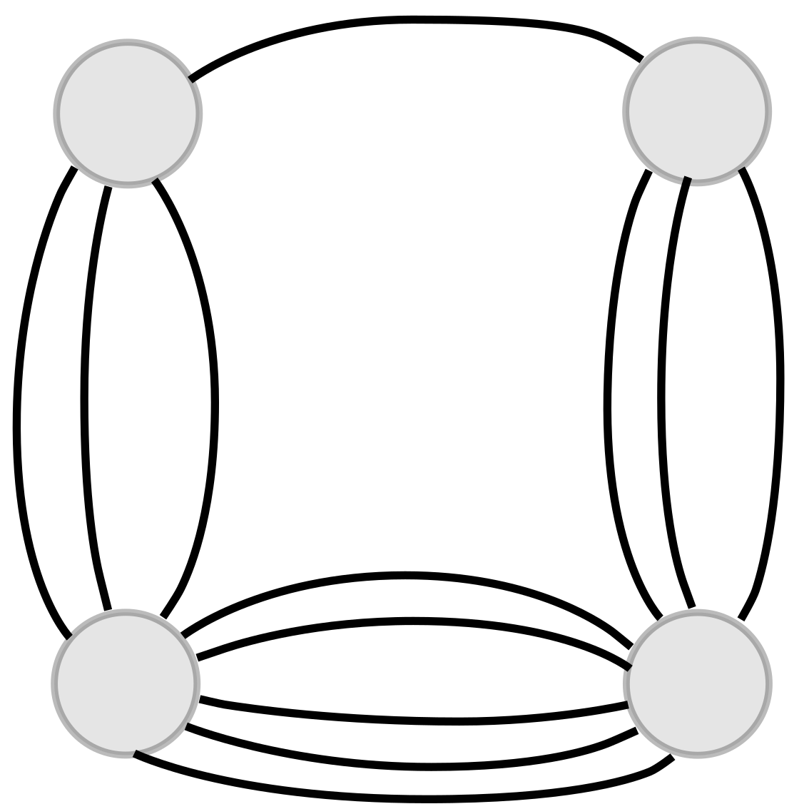
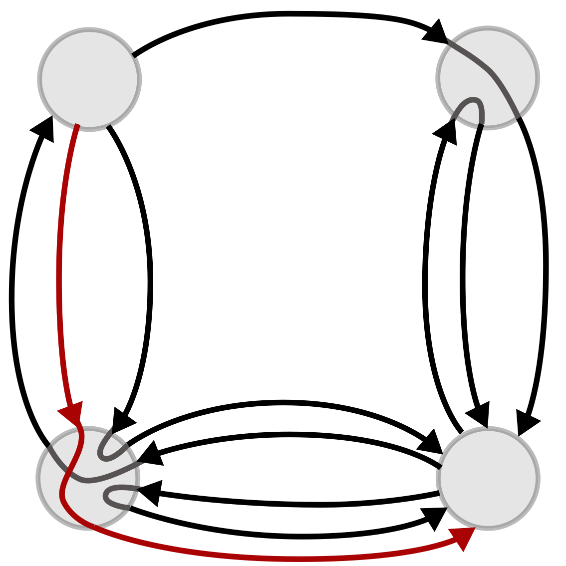
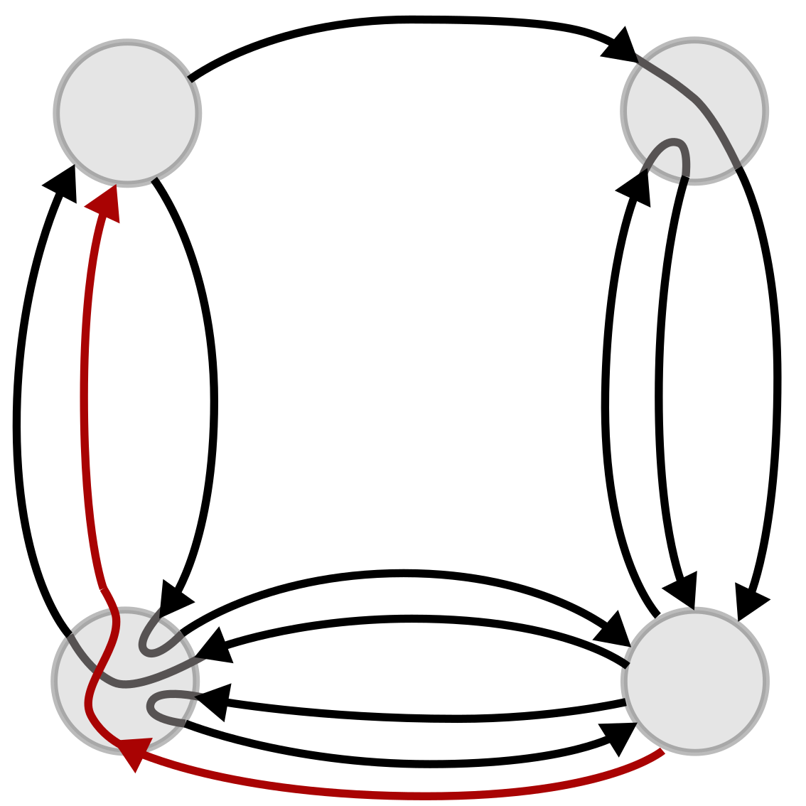
Figure 1. Left to right: an Eulerian multigraph $\mathcal{M}$; a loop configuration $\omega\in\mathcal{L}^{a,b}_{2(\delta_{a}-\delta_{b})}$ on $\mathcal{M}$ ($a$ is the top left and $b$ the bottom right vertex) together with a path from $a$ to $b$ marked red; a loop configuration $\omega^{\prime}\in\mathcal{L}^{a,b}_{0}$ with the path reversed; and one of the final loop configurations $\omega^{\prime\prime}\in\mathcal{L}^{\emptyset}_{0}$ corresponding to $\omega^{\prime}$, i.e., such that $\rho(\omega^{\prime\prime})=\omega^{\prime}$.

Let us finish with a number of remarks.

Remark 3.

We stress again that the crucial property of this loop representation is that the measure ${\mathbf{P}}_{G,\beta}$ is supported on collections of closed loops, and is independent of the choice of $a$ and $b$. A similar idea was used by Lees and Taggi [LeeTag] to study spin $O(n)$ models with an external magnetic field. Moreover, by Proposition 7 and Lemma 8, the random loops under ${\mathbf{P}}_{G,\beta}$ carry probabilistic information about both the spin XY model (in terms of correlation functions) and its dual height function (as an exact coupling). An analogous role for the Ising and Ashkin–Teller model is played by the (double) random current measure that encodes both an integer valued height function and the spin correlations [DCL, Lis19, LisAT]. The difference is that for the XY model, the correlations are determined by loop connectivities instead of percolation connectivities. This comparison offers an alternative explanation for the different types of phase transition in discrete and continuous spin systems.

Remark 4.

The approach above is different from [Sym, BFS, BenUel, LeeTag] in that in the loop configurations, we never make connections at vertices with sources. This leads to different combinatorics than in [BenUel], and in particular a more transparent formula for the two-point function. See also Appendix A for a different construction where we allow such connections.

Remark 5.

We call a multigraph $\mathcal{M}$ Eulerian if its degree is even at every vertex. Another way to sample the loop configuration that easily follows from the above definitions is the following procedure:

• First sample an Eulerian submultigraph $\mathcal{M}$ of $G$ with probability proportional to

  $$\mathcal{E}(\mathcal{M})\prod_{e\in E}\frac{1}{\mathcal{M}_{e}!}\Big{(}\frac{\beta}{2}\Big{)}^{\mathcal{M}_{e}},$$

  where $\mathcal{E}(\mathcal{M})$ is the number of Eulerian orientations of $\mathcal{M}$, i.e., assignments of orientations to every edge of $\mathcal{M}$ with an equal number of incoming and outgoing edges at every vertex.

• Then choose uniformly at random an Eulerian orientation of $\mathcal{M}$.

• Finally, at each vertex, independently of other vertices, connect the incoming edges with the outgoing edges uniformly at random.

Remark 6.

Using the same argument as above one obtains the following formula for higher power two-point functions. For $k\geq 1$, we have

$$\langle\sigma^{2k}_{a}\bar{\sigma}^{2k}_{b}\rangle_{G,\beta}={\mathbf{E}}_{G,\beta}\Big{[}\frac{(m_{a,b})_{k}}{(m_{a,b}+k)_{k}}\Big{]},$$

where $(m)_{k}=m(m-1)\cdots(m-k+1)$ is the falling factorial. One can also consider multi-point functions and get more complicated loop representation formulas.

Remark 7.

This representation is valid on any, not necessarily planar, graph, and it is known that the XY model exhibits long-range order in dimension greater than two [FSS]. The disorder-order transition should coincide with the onset of infinite loops (biinfinite paths) on the current. The alternative heuristic for the lack of symmetry breaking in two dimensions arising from this picture is that planar simple random walk is recurrent (an hence does not produce infinite loops).

Remark 8.

The isomorphism theorem of Le Jan [LeJan] says that the discrete complex Gaussian free field can be coupled with a Poissonian collection of random walk loops, the so called random walk loop soup, in such a way that one half of the square of the absolute value of the field is equal to the total occupation time of the random walk loops. On the other hand, it is immediate that conditioned on the absolute value of the field, its complex phase is distributed like the XY model with coupling constants depending on this absolute value. With some work, e.g. using [LeJan1], one can show that under this conditioning the random walk loops have the same distribution as the loops described above.

4. Delocalisation implies no exponential decay

In this section we prove that if the height function delocalises, then the spin correlations are not summable along certain sets of vertices. In the next section, we will show how to apply this together with the delocalisation results of Lammers [Lammers] to deduce a BKT-type phase transition in a wide range of periodic planar graphs.

Suppose $\Gamma=(V,E)$ is a translation invariant planar graph, and write

$$\langle\sigma_{a}\bar{\sigma}_{b}\rangle_{\Gamma,\beta}=\lim_{G\nearrow\Gamma}\langle\sigma_{a}\bar{\sigma}_{b}\rangle_{G,\beta}$$ (12)

for the infinite volume two-point function, where the limit is taken along any increasing sequence of subgraphs $G$ exhausting $\Gamma$. That this is well defined is guaranteed by the fact that the sequence is nondecreasing, i.e., $\langle\sigma_{a}\bar{\sigma}_{b}\rangle_{G,\beta}\leq\langle\sigma_{a}\bar{\sigma}_{b}\rangle_{G^{\prime},\beta}$ if $G$ is a subgraph of $G^{\prime}$, which in turn is a classical consequence of the Ginibre inequality [Gin].

Definition.

Let $0$ be a distinguished face of $\Gamma$. A bi-infinite self-avoiding path in $\Gamma$ that goes through at least one edge incident to $0$ is called a cut (at $0$). Note that a cut $L$ naturally splits into two infinite sets of vertices $L_{+}$ and $L_{-}$ with the property that any cycle in $\Gamma$ that surrounds $0$ must intersect both $L_{+}$ and $L_{-}$.

The main quantity of interest for us will be the sum of correlations along cuts. To be more precise for $\varepsilon>0$, let

$$\chi^{\epsilon}_{\Gamma,\beta}(L)=\sum_{a\in L_{+},b\in L_{-}}(\langle\sigma_{a}\overline{\sigma}_{b}\rangle_{\Gamma,\beta})^{2-\varepsilon}.$$ (13)

Proposition 9.

For every $\epsilon>0$, there exists $C=C(\epsilon,\beta,\Gamma)<\infty$ such that for all finite subgraphs $G$ of $\Gamma$ containing $0$, we have

$$\mathbb{E}_{G,\beta}[|h(0)|]\leq C\inf_{L}\chi^{\epsilon}_{\Gamma,\beta}(L),$$

where the infimum is over all cuts at $0$.

Before presenting the proof, let us mention that a direct corollary of this proposition is the following. A natural example of a cut is any path that stays at a constant distance from a straight line going through $0$. In this case it is easy to see that $\chi^{\epsilon}_{\Gamma,\beta}(L)$ is finite whenever there is exponential decay of spin correlations. We can now state the main conclusion of this section.

Corollary 10.

If the height function delocalises in the sense of Theorem 3, then

$$\chi^{\epsilon}_{\Gamma,\beta}(L)=\infty$$

for all $\varepsilon>0$ and all cuts $L$ at $0$. In particular the two-point function does not decay exponentially fast with the distance between the vertices.

Proof.

We know that situation $(i)$ from Theorem 3 does not happen. This means that $\sup_{n}\mathbb{E}_{B_{n},\beta}[|h(0)|]=\infty$, and the claim follows directly from Proposition 9. ∎

Remark 9.

One naturally expects that the localisation-delocalisation phase transition for the height function happens at the same temperature as the BKT transition for the XY model. The remaining part of this prediction is therefore to show that if the spin correlations do not decay exponentially, then the height function delocalises. We do not do this in this article.

Recall that $m_{a,b}$ is the number of paths (pieces of loops) in a loop configuration that go from $a$ to $b$. We will need the following lemma.

Lemma 11.

For all $\beta>0$ and $p>1$, there exists a $C_{p}<\infty$ such that for all finite graphs $G=(V,E)$ and all $a,b\in V$,

$$\mathbf{E}_{G,\beta}[m_{a,b}]\leq C_{p}\deg_{G}(a)\big{(}\mathbf{P}_{G,\beta}(m_{a,b}>0)\big{)}^{\frac{1}{p}}.$$

Proof.

Fix $\beta>0$, $G=(V,E)$ and $a,b\in V$, and let $\omega\in\mathcal{L}_{0}$ be a loop configuration on $G$. Denote by $\omega_{e}$, the number of visits of all loops in $\omega$ to an undirected edge $e\in E$. If there are $m\geq 1$ paths going from $a$ to $b$ in $\omega$, then in particular $\sum_{c\sim a}\omega_{\{a,c\}}\geq m$. This implies that

$$\mathbf{E}_{G,\beta}[m_{a,b}]\leq\mathbf{E}_{G,\beta}\Big{[}\sum_{c\sim a}\omega_{\{a,c\}}\mathds{1}\{m_{a,b}>0\}\Big{]}\leq\deg_{G}(a)\max_{c\sim a}\mathbf{E}_{G,\beta}[\omega_{\{a,c\}}\mathds{1}\{m_{a,b}>0\}].$$

Applying Hölder’s inequality gives

$$\mathbf{E}_{G,\beta}[\omega_{\{a,c\}}\mathds{1}\{m_{a,b}>0\}]\leq\big{(}\mathbf{E}_{G,\beta}[\omega_{\{a,c\}}^{q}]\big{)}^{1/q}\mathbf{P}_{G,\beta}(m_{a,b}>0)^{1/{p}},$$

where $1/p+1/q=1$. We now notice that by definition, $\omega_{e}$ under $\mathbf{P}_{G,\beta}$ has the same distribution as the amplitude $|\mathbf{n}|_{e}$ under $\mathbb{P}_{G,\beta}$. Therefore, to finish the proof it is enough to show that for all $p>1$, there exists $C_{p}<\infty$ depending on $\beta$ but independent of $G$ such that

$$\mathbb{E}_{G,\beta}[|\mathbf{n}|^{p}_{e}]\leq C_{p}.$$ (14)

We postpone the proof of this bound to Lemma 13 and Lemma 14. ∎

The last ingredient that we will need is the following inequality

Lemma 12.

For any $a,b\in V$, we have

$$\langle\sigma^{2}_{a}\bar{\sigma}^{2}_{b}\rangle_{G,\beta}\leq 2\langle\sigma_{a}\bar{\sigma}_{b}\rangle^{2}_{G,\beta}.$$

Proof.

A version of the Ginibre inequality (see e.g. [BLU]) says that

$$\big{\langle}\Im(\sigma_{a})\Im(\sigma_{b})\Re(\sigma_{a})\Re(\sigma_{b})\big{\rangle}_{G,\beta} \leq\big{\langle}\Im(\sigma_{a})\Im(\sigma_{b})\big{\rangle}_{G,\beta}\big{\langle}\Re(\sigma_{a})\Re(\sigma_{b})\big{\rangle}_{G,\beta}.$$

which after rearrangement gives the desired inequality. ∎

We note that the constant in the inequality above can be improved to $1$ using our switching techniques from Appendix A (see Remark 10).

We are now ready to prove the main theorem.

Proof of Proposition 9.

Fix a finite subgraph $G$ and a cut $L$. By Proposition 7 the height function $h(0)$ under $\mathbb{P}_{G,\beta}$ has the sam law as $W(0)$ – the total net winding around $0$ of all loops in a loop configuration – drawn according to $\mathbf{P}_{G,\beta}$. Moreover, any piece of a loop that adds to the winding (in any orientation) must intersect both $L_{+}$ and $L_{-}$ by definition of a cut. Therefore, taking $p=2/(2-\varepsilon)$, we have

$$\mathbb{E}_{G,\beta}[|h(0)|] =\mathbf{E}_{G,\beta}[|W(0)|]$$

$$\leq\sum_{a\in L_{+},b\in L_{-}}\mathbf{E}_{G,\beta}[m_{a,b}]$$

$$\leq\tilde{C}\sum_{a\in L_{+},b\in L_{-}}(\mathbf{P}_{G,\beta}(m_{a,b}>0))^{1/p}$$

$$\leq 2\tilde{C}\sum_{a\in L_{+},b\in L_{-}}(\langle\sigma^{2}_{a}\bar{\sigma}^{2}_{b}\rangle_{G,\beta})^{1-\varepsilon/2}$$

$$\leq 4\tilde{C}\sum_{a\in L_{+},b\in L_{-}}(\langle\sigma_{a}\bar{\sigma}_{b}\rangle_{G,\beta})^{2-\varepsilon}$$

$$\leq C\chi^{\epsilon}_{\Gamma,\beta}(L).$$

where the third line follows from Lemma 11, the forth one from Lemma 8, the fifth one from Lemma 12, and the last one from (12). This completes the proof. ∎

It therefore remains to show (14), which will directly follow from Lemma 13 and Lemma 14 below. To that end, define for $k\in\mathbb{N}$ and $\beta>0$, a random variable $Y_{k}$ by

$$\mathbb{P}_{\beta}(Y_{k}=i)\propto\frac{1}{i!(i+k)!}\big{(}\tfrac{\beta}{2}\big{)}^{2i+k},$$

so that the normalizing constant is $I_{k}(\beta)$. For $e=vv^{\prime}$, let

$$|\nabla h|_{e}=|\mathbf{n}_{(v,v^{\prime})}-\mathbf{n}_{(v^{\prime},v)}|$$

be the absolute value of the gradient of the height function across the dual edge $e^{\dagger}$. Note that the random variables $(X_{e}=X_{e}(\mathbf{n}))_{e\in E}$ defined through

$$X_{e}=\frac{|\mathbf{n}|_{e}-|\nabla h|_{e}}{2}$$

have the same distribution as $Y_{|\nabla h|_{e}}$. Moreover, conditionally on $|\nabla h|$, they are an independent family. To show (14) it is enough to bound the moments of $|\nabla h|_{e}$ and $X_{e}$ separately, which we will now do.

Lemma 13.

For all $\beta>0$ and all $r\in\mathbb{N}$, there exists a $C_{r}<\infty$ such that for all finite planar graphs $G=(V,E)$ and all $e\in E$,

$$\mathbb{E}_{G,\beta}[|\nabla h|_{e}^{r}]\leq C_{r}.$$

Proof.

Fix a finite planar graph $G$, and let $e=vv^{\prime}\in E$. We write $G\setminus e$ for the graph without the edge $e$. For $l\in\mathbb{Z}$, we define $\Omega_{l}(G)=\{\mathbf{n}\text{ on }G:\delta\mathbf{n}=l(\delta_{v}-\delta_{v^{\prime}})\}$, and

$$Z^{l}_{G}=\sum_{\mathbf{n}\in\Omega_{r}(G)}w_{\beta}(\mathbf{n}),$$

and analogously $Z^{l}_{G\setminus e}$. Similarly to (11), we get from the current expansion of correlation functions that

$$\langle\sigma_{v}^{l}\bar{\sigma}_{v^{\prime}}^{l}\rangle_{G\setminus e,\beta}=\frac{Z_{G\setminus e}^{l}}{Z^{0}_{G\setminus e}}.$$

By the definition of the height function and currents, we therefore have

$$\mathbb{P}_{G,\beta}(|\nabla h|_{e}=l)=I_{l}(\beta)\frac{(Z^{l}_{G\setminus e}+Z^{-l}_{G\setminus e})}{Z^{0}_{G}}=2I_{l}(\beta)\frac{Z^{l}_{G\setminus e}}{Z^{0}_{G\setminus e}}\frac{Z^{0}_{G\setminus e}}{Z^{0}_{G}}\leq 2I_{l}(\beta)\leq 2I_{0}(\beta)\frac{\beta^{l}}{2^{l}l!},$$

where we used the obvious bounds $\langle\sigma_{v}^{l}\bar{\sigma}_{v^{\prime}}^{l}\rangle_{G\setminus e,\beta}\leq 1$, and ${Z^{0}_{G\setminus e}}/{Z^{0}_{G}}\leq 1$, and the last inequality follows easily from the definition of $I_{r}(\beta)$. Finally,

$$\mathbb{E}_{G,\beta}[|\nabla h|_{e}^{r}] =\sum_{l\geq 1}l^{r}\mathbb{P}_{G,\beta}(|\nabla h|_{e}=l)\leq 2I_{0}(\beta)\sum_{l\geq 1}l^{r}\frac{\beta^{l}}{2^{l}l!}=:C_{r}<\infty.$$

The last bound is independent of $G$ and $e$ which completes the proof. ∎

Lemma 14.

For all $\beta>0$ and all $r\in\mathbb{N}$, there exists a $\tilde{C}_{r}<\infty$ such that for all finite planar graphs $G=(V,E)$ and $e\in E$,

$$\mathbb{E}_{G,\beta}[|X_{e}|^{r}]\leq\tilde{C}_{r}.$$

Proof.

For two nonnegative integers $i,r$, let $(i)_{r}=i(i-1)\cdots(i-r+1)$ be the falling factorial with the convention that $(i)_{0}=1$. Note that $(i)_{r}=0$ whenever $i<r$. It will be convenient to look at the falling factorial moments. First note that by definition of $Y_{k}$,

$$\mathbb{E}_{\beta}[(Y_{k})_{r}] =\frac{1}{I_{k}(\beta)}\sum_{i\geq 0}\frac{(i)_{r}}{i!(i+k)!}\big{(}\tfrac{\beta}{2}\big{)}^{2i+k}=\frac{\big{(}\tfrac{\beta}{2}\big{)}^{r}}{I_{k}(\beta)}\sum_{i\geq 0}\frac{1}{i!(i+k+r)!}\big{(}\tfrac{\beta}{2}\big{)}^{2i+k+r}=(\tfrac{\beta}{2}\big{)}^{r}\frac{I_{k+r}(\beta)}{I_{k}(\beta)}.$$

By the Turán inequality (5), the map $k\mapsto I_{k+1}(\beta)/I_{k}(\beta)$ is decreasing and hence

$$\mathbb{E}_{\beta}[(Y_{k})_{r}]=\big{(}\tfrac{\beta}{2}\big{)}^{r}\frac{I_{k+r}(\beta)}{I_{k}(\beta)}\leq\big{(}\tfrac{\beta}{2}\big{)}^{r}\frac{I_{r}(\beta)}{I_{0}(\beta)}=:C.$$

Now note that $(i)_{r}\geq|i-r|^{r}$ when $i\geq r$, and hence $i^{r}\leq 2^{r-1}(|i-r|^{r}+r^{r})\leq 2^{r}((i)_{r}+r^{r})$. Finally

$$\mathbb{E}_{\beta}[|X_{e}|^{r}\mid|\nabla h|_{e}=k]=\mathbb{E}_{\beta}[|Y_{k}|^{r}]\leq 2^{r}(C+r^{r}):=\tilde{C}_{r},$$

where the last bound does not depend on $k$. Integrating over the possible values of $|\nabla h|_{e}$ concludes the proof. ∎

5. Existence of phase transition in the XY model

In this section, we prove that for all translation invariant planar graphs $\Gamma=(V,E)$, the XY model undergoes a non-trivial phase transition in terms of the quantity $\chi^{\varepsilon}_{\beta}(L)$. As before, let $0$ denote an arbitrary distinguished face of $\Gamma$. We define

$$\beta_{0}=\inf\{\beta>0:\text{for all ${\varepsilon>0}$ and all cuts $L$ at $0$, $\chi^{\varepsilon}_{\beta}(L)=\infty$}\}.$$

Theorem 15.

Let $\Gamma$ be as above. Then $\beta_{0}<\infty$.

By Corollary 10 it is enough to show that for any such $\Gamma$, there exists a finite $\beta_{0}>0$ such that the associated height function delocalises in the sense that there are no translation invariant Gibbs measures on the dual $\Gamma^{\dagger}$. We first implement this strategy for triangulations, where delocalisation can be shown directly using the general result of Lammers [Lammers] (Theorem 2).

Proof of Theorem 15 for triangulations.

Let $\Gamma$ be a translation invariant triangulation. Note that condition (6) in our case is equivalent to ${I_{1}(\beta)}/{I_{0}(\beta)}\geq\frac{1}{2}$. It is known that this fraction converges to $1$ as $\beta\to\infty$ (see for example [Segura]), and therefore in light of Theorem 2, there are no translation invariant Gibbs measures for $\beta$ large enough. ∎

To extend beyond triangulations, we will use a different approach. We stress that in particular, we will not show delocalisation of the height function on graphs that are not triangulations. Instead, we exploit monotonicity in coupling constants to bound from below the spin correlations on an arbitrary translation invariant graph by correlations on a modified graph that is a triangulation. We explain this procedure in detail for the square lattice, and briefly mention the extension to other lattices at the end.

In what follows, we will need the following well known monotonicity of spin correlations that is a classical consequence of the Ginibre inequality [Gin].

Lemma 16.

For each (infinite or finite) graph $G=(V,E)$, $\beta>0$, and $e\in E$, the function

$$J_{e}\mapsto\langle\sigma_{v}\bar{\sigma}_{v^{\prime}}\rangle_{G,\beta}$$

is nondecreasing.

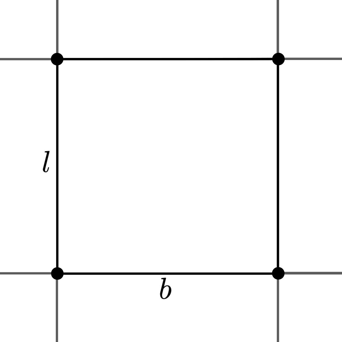
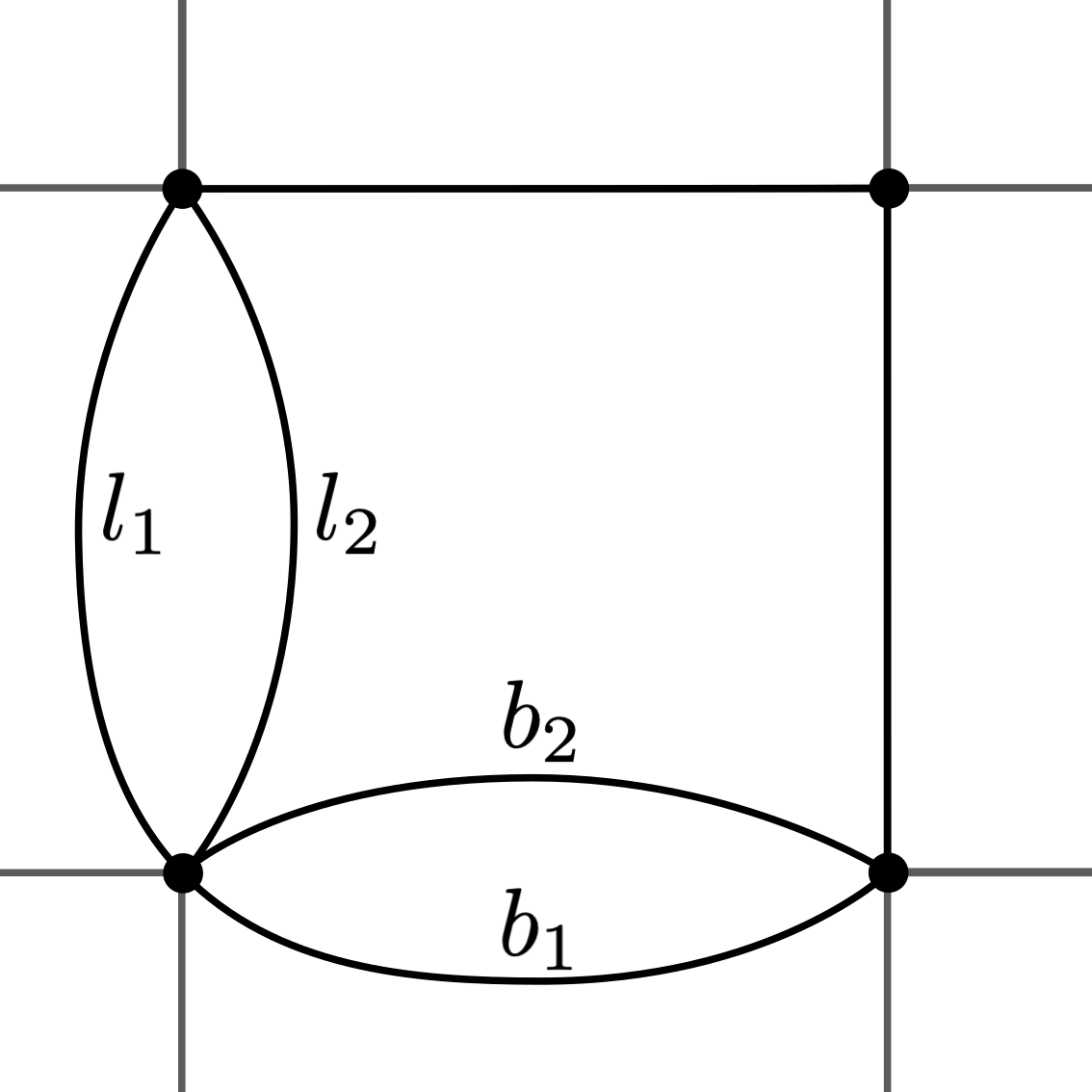
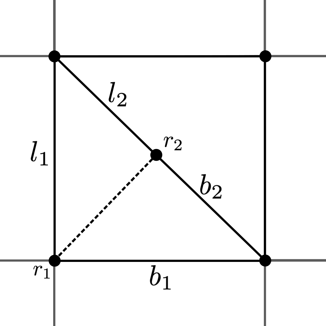
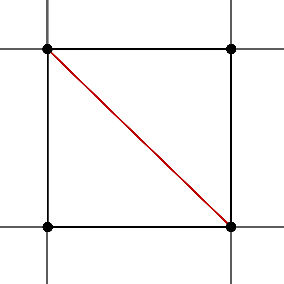
Figure 2. The transformation to a triangulation. The red edge on the right is the edge with different potential.

Proof of Theorem 15 for the square lattice.

Let $\Gamma=(V,E)$ denote the square lattice.

In order to use (6), we need to transform $\Gamma$ into a triangulation. See Figure 2 for guidance. Fix a square and double the bottom and left edge and put coupling constants $\beta/2$ on the doubled edges instead of $\beta$. Next, double the common vertex of the left and bottom edge and add an additional edge $e$, on which we set the coupling constant to infinity. This does not change the distribution of the spins. Finally, set the coupling constant on the edge $e$ to $0$, which is equivalent to removing the edge from the square, and repeat the procedure for all other squares. In this way, we obtain a new lattice $\Gamma^{\prime}$, which consists of squares with a diagonal on which there is an additional vertex. Note that all coupling constants are now equal to $\beta/2$. By Lemma 16,

$$\langle\sigma_{a}\bar{\sigma}_{b}\rangle_{\Gamma,\beta}\geq\langle\sigma_{a}\bar{\sigma}_{b}\rangle_{\Gamma^{\prime},\beta/2}$$ (15)

for all pairs of vertices $a,b$ in $\Gamma$, using the natural embedding of $\Gamma$ on $\Gamma^{\prime}$.

Since $\Gamma^{\prime}$ is a translation invariant graph, the dichotomy statement of Theorem 3 holds. To show that there are no translation invariant Gibbs measures for the associated height function, notice that the dual $(\Gamma^{\prime})^{\dagger}$ of $\Gamma^{\prime}$ (after collapsing the doubled edges to a single edge) is trivalent. Moreover, the height function on any finite subgraph of $(\Gamma^{\prime})^{\dagger}$ has a potential given by $\mathcal{V}_{e}^{\prime}=\mathcal{V}^{\beta/2}_{e}$ for the nondiagonal edges and $\mathcal{V}^{\prime}_{e}=2\mathcal{V}^{\beta/2}_{e}$ otherwise, and the potential $\mathcal{V}^{\prime}$ satisfies Lammers’ condition (6) precisely when $\left({I_{1}(\beta/2)}/{I_{0}(\beta/2)}\right)^{2}\geq\frac{1}{2}$. Since the fraction on the left-hand side tends to $1$ as $\beta\to\infty$, we can choose $\beta$ large enough so that there are no translation invariant Gibbs measures for the height function on $(\Gamma^{\prime})^{\dagger}$.

Note that every cut on $\Gamma$ embeds naturally as a cut on $\Gamma^{\prime}$. Therefore, by Proposition 9 together with (15), we have that for each cut $L$ on $\Gamma$ and each $\epsilon>0$,

$$\chi_{\Gamma,\beta}^{\epsilon}(L)\geq\chi_{\Gamma^{\prime},\beta/2}^{\epsilon}(L)=\infty.$$

This finishes the proof. ∎

To extend this proof to general graphs, we make each face into a triangulation by “zig-zagging” (see Figure 3).

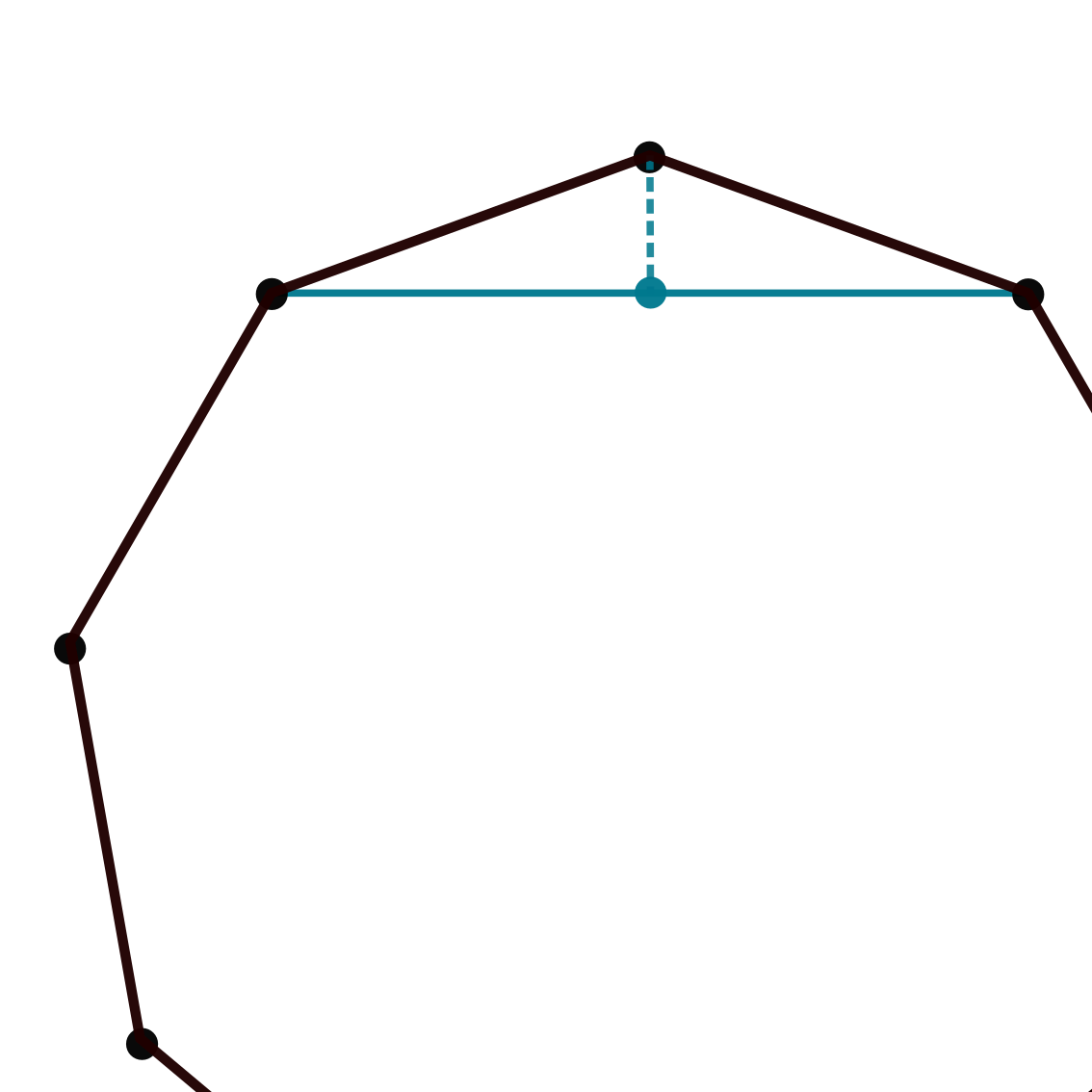
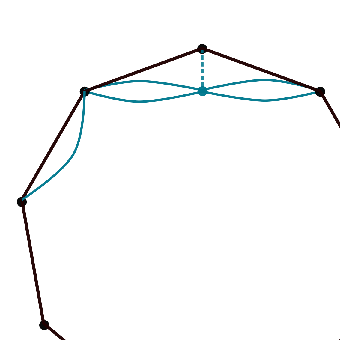
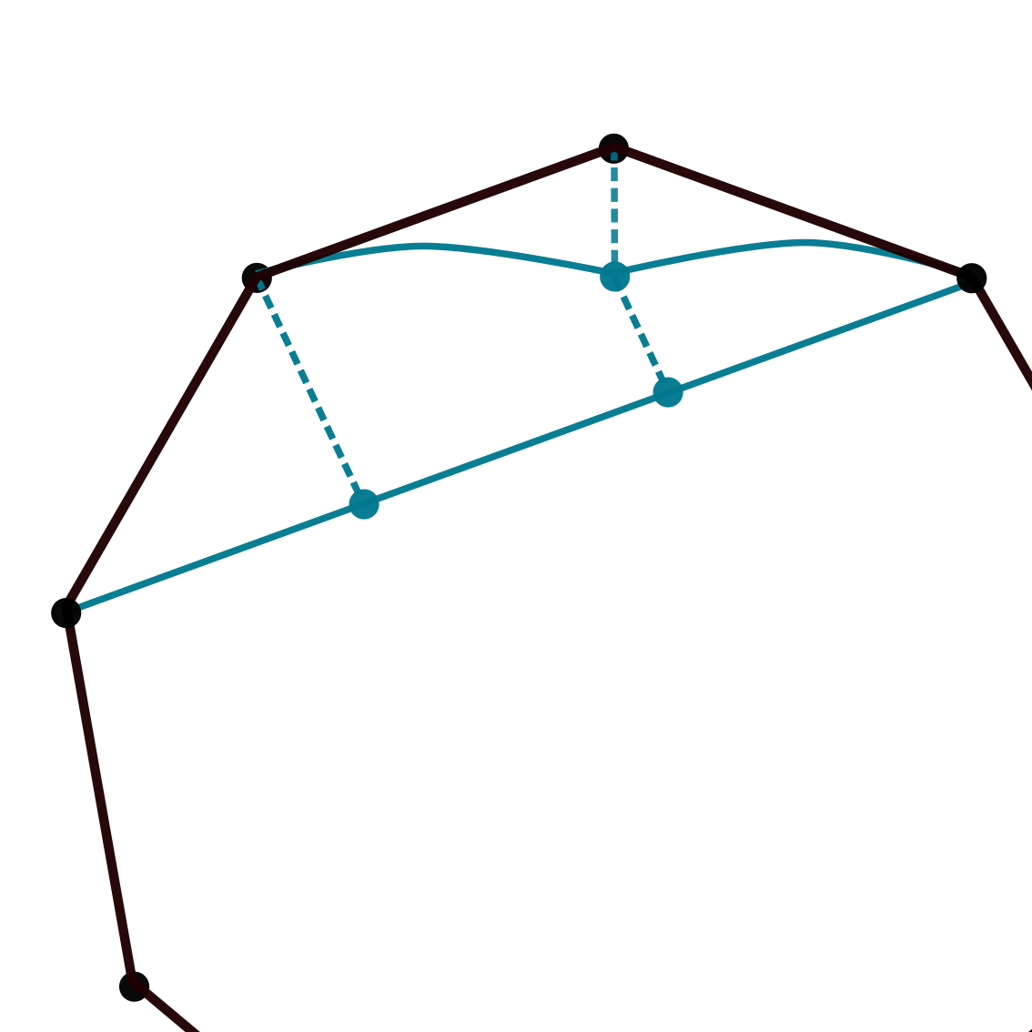
Figure 3. The transformation of a general graph to a triangulation (after identifying the resulting multiple edges). The dashed edges are such that the coupling constant is set to infinity first, and then to zero (which is equivalent to removing the edges) and hence the spin correlations in the final graph are smaller than in the original graph.

6. No exponential decay implies a power-law lower bound

In this section we finish the proof of the main theorem by showing that the absence of exponential decay implies a power-law lower bound on the two-point function when $\Gamma=\mathbb{Z}^{2}$. Similar arguments can be applied to other graphs that in addition to being translation invariant possess reflection and rotation symmetries.

Proof of Theorem 1.

Let $0$ denote the vertex at the origin. For a finite subgraph $G$ of $\mathbb{Z}^{2}$ containing $0$, let

$$\varphi_{G,\beta}=\sum_{w\in\partial G}\langle\sigma_{0}\bar{\sigma}_{w}\rangle_{G,\beta},$$

where $\partial G$ is the set of vertices of $G$ adjacent to at least one vertex outside $G$. Define

$$\beta_{c}=\sup\{\beta:\text{there exists finite $G$ with $\varphi_{G,\beta}<1$}\}.$$ (16)

We will show that $\beta_{c}$ satisfies the properties listed in Theorem 1. To this end first fix $\beta<\beta_{c}$. By Lemma 16, there exists a finite graph $G$ with $\varphi_{G,\beta}<1$. Using a standard argument that consists in iteratively applying the Lieb–Rivasseau inequality [Lieb, Riv] (see Lemma 20) to translates of $G$, we obtain that the two-point functions decay exponentially fast, and hence (i) holds true.

To conclude (ii), note that for each finite $G$, $\varphi_{G,\beta}$ is a continuous function of $\beta$, and hence the set in (16) is open. This means that for every $\beta\geq\beta_{c}$, we have $\varphi_{G,\beta}\geq 1$ for all finite subgraphs $G$.

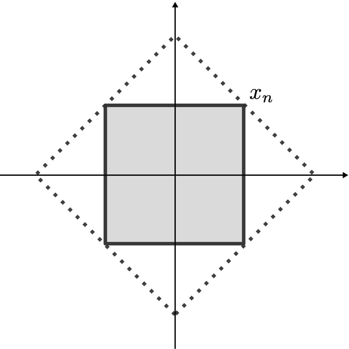
Figure 4. The $[-n,n]^{2}$ box $\Lambda_{n}$ shaded in grey and the $L^{1}$ ball $\Lambda^{\prime}_{n}$ of radius $2n$.

Now let $\Lambda_{n}$ be the box $[-n,n]^{2}$, and let $\Lambda^{\prime}_{n}$ be the ball in $L^{1}$ of radius $2n$ (see Figure 4). We write $x_{n}:=(n,n)\in\partial\Lambda_{n}\cap\partial\Lambda^{\prime}_{n}$ and $a_{n}=\langle\sigma_{0}\bar{\sigma}_{x_{n}}\rangle_{\mathbb{Z}^{2},\beta}$. By rotation symmetry and the Messager–Miracle-Sole [MMS] inequality (see Lemma 21), we have

$$a_{n}=\min_{v\in\partial\Lambda_{n}}\langle\sigma_{0}\bar{\sigma}_{v}\rangle_{\mathbb{Z}^{2},\beta}=\max_{v\in\partial\Lambda^{\prime}_{n}}\langle\sigma_{0}\bar{\sigma}_{v}\rangle_{\mathbb{Z}^{2},\beta}.$$

For $\beta\geq\beta_{c}$, we moreover have

$$\sum_{w\in\partial\Lambda^{\prime}_{n}}\langle\sigma_{0}\overline{\sigma}_{w}\rangle_{\mathbb{Z}^{2},\beta}\geq\varphi_{\Lambda_{n}^{\prime},\beta}\geq 1.$$

These two observations together imply that for any $v\in\partial\Lambda_{n}$,

$$\langle\sigma_{0}\bar{\sigma}_{v}\rangle_{\mathbb{Z}^{2},\beta}\geq a_{n}\geq\frac{1}{|\partial\Lambda^{\prime}_{n}|}=\frac{1}{8n}\geq\frac{1}{8|v|}$$

which implies $(ii)$.

Finally by Theorem 15 we know that there exists a finite $\beta$ at which there is no exponential decay, and by classical expansions there exists a nonzero $\beta$ at which there is exponential decay (see e.g. [AizSim]). We conclude that $0<\beta_{c}<\infty$. ∎

Appendix A Double currents, path switching and correlation inequalities

The main purpose of this section is to present a new technique that may be applied to a further study of the XY model (possibly in higher dimensions). We develop a loop representation for squares and products of correlation functions. This is a generalization of the construction from Section 3, and to the best of our knowledge has not yet been described in the literature. It is also analogous to the double random current representation of the Ising model [GHS, aizenman, ADCS] but is more subtle as one has to deal with path switching rather than connection switching in a percolation model. We stress the fact that we do not use any of the results from this section in the proof of the main theorem, except for the well known inequalities of Lieb and Rivasseau, and Messager and Miracle-Sole.

There will be two major differences in the definition of a loop configuration compared to Section 3: the edges will come in two colours, red and blue, corresponding to two currents $\mathbf{r}$ and $\mathbf{b}$ respectively, and we will allow the paths to enter vertices $v$ at which the number of incoming and outgoing edges is not the same, i.e., $\delta(\mathbf{r}+\mathbf{b})_{v}\neq 0$. To be more precise, consider the following definition.

Definition (Coloured loop configurations outside $S$ with sources $\varphi$).

Let $\mathcal{M}$ be a multigraph on $V$, let $S\subseteq V$, and $\varphi:V\to\mathbb{Z}$ with $\sum_{v\in V}\varphi_{v}=0$. A coloured loop configuration (on $\mathcal{M}$) outside $S$ with sources $\varphi$ is

• an assignment of a red or blue color to each edge of $\mathcal{M}$, together with

• a collection of

  • unrooted directed loops on $\mathcal{M}$ avoiding $S$, and

  • directed open paths on $\mathcal{M}$ not visiting $S$ except possibly at their start and end vertex,

  such that

  • every edge of $\mathcal{M}$ is traversed exactly once by a loop or a path, and

  • at each vertex $v\in V\setminus S$, there are exactly $\varphi_{v}\mathds{1}\{\varphi_{v}>0\}$ outgoing and $-\varphi_{v}\mathds{1}\{\varphi_{v}<0\}$ incoming paths.

We write $\tilde{\mathcal{L}}^{S}_{\varphi}$ for the set of all coloured loop configurations outside $S$ with sources $\varphi$, and define a weight on $\tilde{\mathcal{L}}^{S}_{\varphi}$ by

$$\tilde{\lambda}^{S}_{\beta}(\omega)=\prod_{v\in V\setminus S}\frac{|\varphi_{v}|!}{((\deg_{\mathcal{M}}(v)+|\varphi_{v}|)/2)!}\prod_{e\in E}\frac{1}{\mathcal{M}_{e}!}\Big{(}\frac{\beta}{2}\Big{)}^{\mathcal{M}_{e}},$$ (17)

where $\mathcal{M}$ is the underlying multigraph, and $\mathcal{M}_{e}$ is the number of copies of $e$ in $\mathcal{M}$.

Note that this weight no longer only depends on the multigraph $M$ and on $S$, but also on $|\varphi(\omega)|$, where $\varphi(\omega)$ are the sources of $\omega$. Also note that in the above definition $S$ and $\varphi$ can be chosen independently. $S$ denotes the set of vertices where we do not resolve any connections between paths and loops, and $\varphi$ prescribes where the sources and sinks are (vertices with nonzero value of $\varphi$). At any such vertex $v$, we resolve as many connections as possible leaving only $|\varphi_{v}|$ incoming or outgoing arrows unmatched, depending on the sign of $\varphi_{v}$. This is the reason why $\varphi$ appears in the above weight, which was not the case in Section 3.

As before if $S^{\prime}\subseteq S$, then there is a natural map $\rho:\mathcal{L}^{S^{\prime}}\to\mathcal{L}^{S}$ that consists in forgetting (or cutting) the loop and path connections at the vertices in $S\setminus S^{\prime}$, and

$$\sum_{\tilde{\omega}\in\rho^{-1}[\omega]}\tilde{\lambda}^{S^{\prime}}_{\beta}(\tilde{\omega})=\tilde{\lambda}^{S}_{\beta}(\omega).$$ (18)

Definition (Coloured currents and consistent configurations).

We will consider a pair of currents $\mathbf{r},\mathbf{b}$ that we think of as red and blue respectively. A coloured loop configuration $\omega$ on $\mathcal{M}_{\mathbf{r}+\mathbf{b}}$ is called consistent with $\mathbf{r}$ and $\mathbf{b}$ if for every edge $vv^{\prime}\in E$, the number of times the loops and paths traverse a red (resp. blue) copy of $vv^{\prime}$ in the direction of ${(v,v^{\prime})}$ is equal to $\mathbf{r}_{(v,v^{\prime})}$ (resp. $\mathbf{b}_{(v,v^{\prime})}$). In particular $\omega$ has sources $\delta(\mathbf{r}+\mathbf{b})$. We define $\tilde{{\mathcal{L}}}^{S}_{\mathbf{r},\mathbf{b}}$ to be the set of all coloured loop configurations on $\mathcal{M}_{\mathbf{r}+\mathbf{b}}$ outside $S$ that are consistent with $\mathbf{r}$ and $\mathbf{b}$.

For $\varphi,\psi:V\to\mathbb{Z}$, we also define

$$\tilde{{\mathcal{L}}}_{\varphi,\psi}^{S}=\bigcup_{\mathbf{r}\in\Omega_{\varphi},\mathbf{b}\in\Omega_{\psi}}\tilde{{\mathcal{L}}}^{S}_{\mathbf{r},\mathbf{b}}\subseteq\tilde{{\mathcal{L}}}_{\varphi+\psi}^{S}.$$

where the union is clearly disjoint. For brevity, we will write $\tilde{\mathcal{L}}_{0}^{S}$ instead of $\tilde{\mathcal{L}}_{0,0}^{S}$, where $0$ denotes the zero function on $V$.

We now relate the weights of loops to those of pairs of currents. To this end, note that for each edge $vv^{\prime}\in E$, there are exactly

$$\frac{|\mathbf{r}+\mathbf{b}|_{vv^{\prime}}!}{\mathbf{r}_{(v,v^{\prime})}!\mathbf{r}_{{(v^{\prime},v)}}!\mathbf{b}_{(v,v^{\prime})}!\mathbf{b}_{(v^{\prime},v)}!}$$

ways of assigning colour to the copies of $vv^{\prime}$ in $\mathcal{M}_{\mathbf{r}+\mathbf{b}}$, and to orient them in the two possible ways so that the result is consistent with $\mathbf{r}$ and $\mathbf{b}$. Moreover, independently of the choices of colours and orientations, there are exactly

$$\frac{((\deg_{\mathcal{M}_{\mathbf{r}+\mathbf{b}}}(v)+|\varphi_{v}|)/2)!}{|\varphi_{v}|!}$$

possible pairings of the incoming and outgoing edges at each vertex $v\in V\setminus S$ such that there are exactly $\varphi_{v}\mathds{1}\{\varphi_{v}>0\}$ outgoing and $-\varphi_{v}\mathds{1}\{\varphi_{v}<0\}$ incoming edges unpaired. This is equivalent to choosing the possible steps that all the loops and paths in the configuration make at $v$. Combining all this, we get the following identity:

$$\sum_{\omega\in\tilde{\mathcal{L}}^{S}_{\mathbf{r},\mathbf{b}}}\tilde{\lambda}^{S}_{\beta}(\omega)=w_{\beta}(\mathbf{r})w_{\beta}(\mathbf{b}).$$ (19)

An important observation again is that the right-hand side is independent of $S$, and hence so is the left-hand side.

In particular, for two sourceless currents, we have

$$\sum_{\omega\in\tilde{\mathcal{L}}^{\emptyset}_{0}}\tilde{\lambda}^{\emptyset}_{\beta}(\omega)=\Big{(}\sum_{\mathbf{n}\in\Omega_{0}}w_{\beta}(\mathbf{n})\Big{)}^{2}=(Z^{0}_{G,\beta})^{2}.$$ (20)

Again, in the case when $G$ is planar we get the following distributional identity. Let $\tilde{\mathbf{P}}_{G,\beta}$ to be the probability measure on $\tilde{\mathcal{L}}_{0}:=\tilde{\mathcal{L}}^{\emptyset}_{0}$ induced by the weights $\tilde{\lambda}_{\beta}:=\tilde{\lambda}^{\emptyset}_{\beta}$. For each face $u\in U$ of $G$, and $\omega\in\tilde{\mathcal{L}}_{0}$, define $W_{\omega}(u)$ to be the total net winding of all the loops in $\omega$ around $u$.

Proposition 17.

The law of $(W(u))_{u\in U}$ under $\tilde{\mathbf{P}}_{G,\beta}$ is the same as the law of the sum of two independent height functions $(h(u)+h^{\prime}(u))_{u\in U}$ under ${\mathbb{P}}_{G,\beta}$.

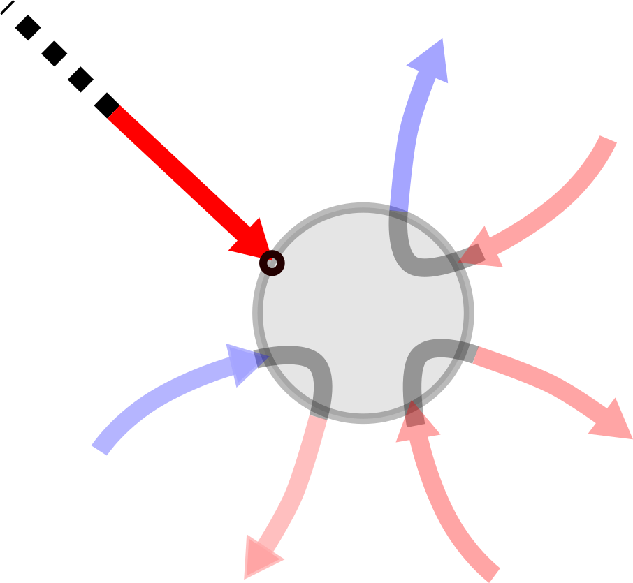
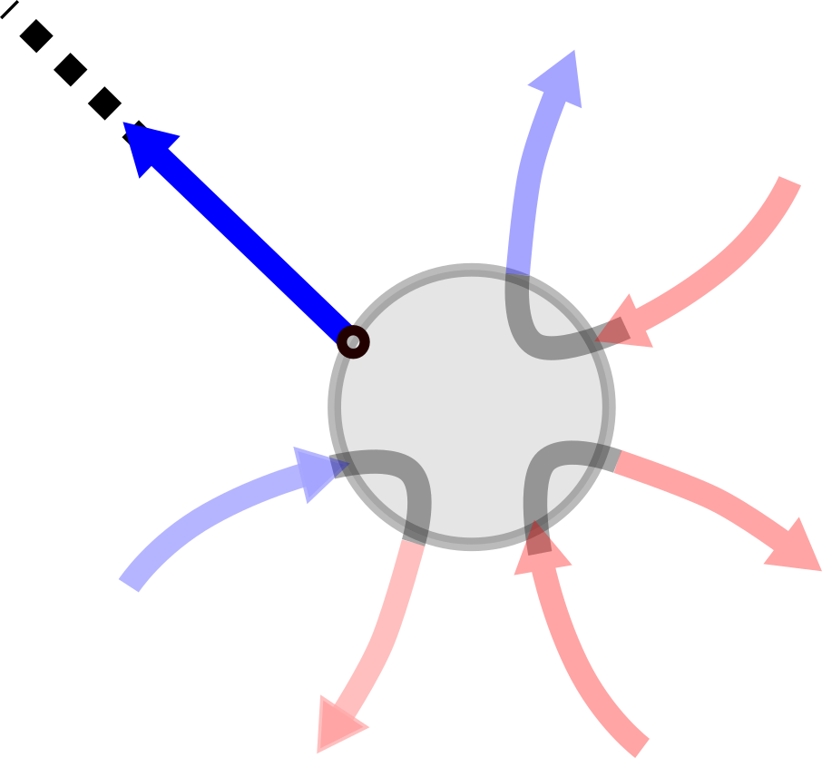
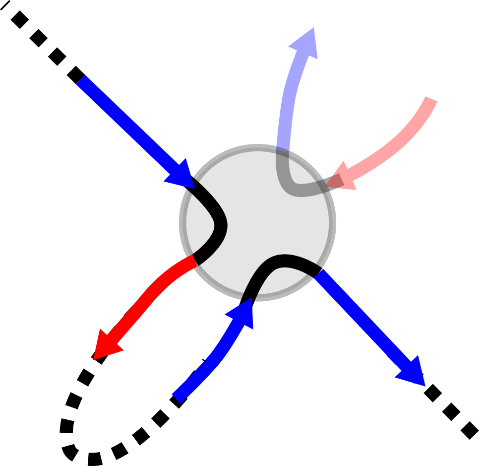
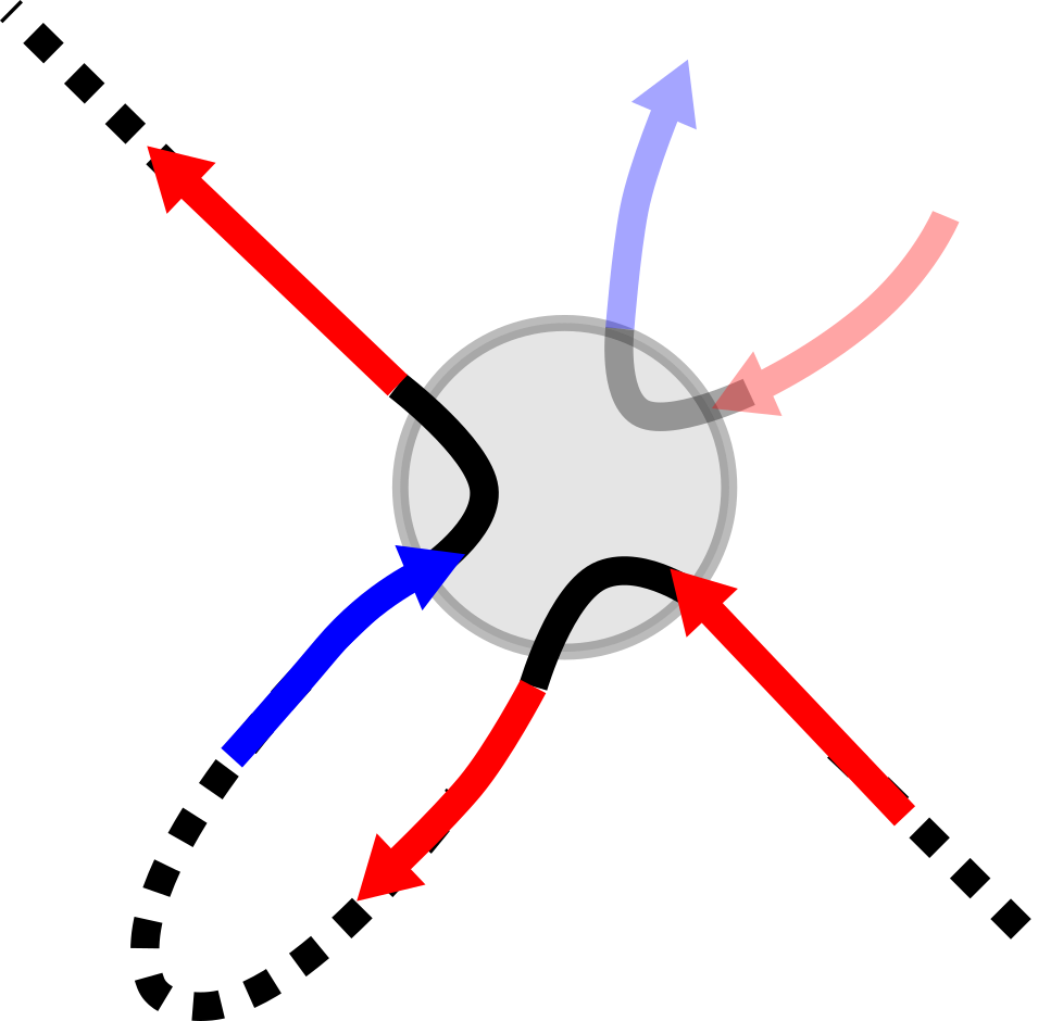
Figure 5. Path switching behaviour at a vertex $v$ that is (resp. is not) the start or end-point of the switched path. Left: the values of both $\delta\mathbf{r}_{v}$ and $\delta\mathbf{b}_{v}$ are increased by one after switching. Right: the values are not changed.

A.1. The two point-function and path switching

We now turn to the loop representation of the square of the two-point function. To this end, write $\varphi=\delta_{a}-\delta_{b}$. Similar to (11), we get

$$\langle\sigma_{a}\bar{\sigma}_{b}\rangle^{2}_{G,\beta}=\Bigg{(}\frac{\sum_{\mathbf{n}\in\Omega_{\varphi}}w_{\beta}(\mathbf{n})}{Z^{0}_{G,\beta}}\Bigg{)}^{2}=\frac{\sum_{\mathbf{r},\mathbf{b}\in\Omega_{\varphi}}w_{\beta}(\mathbf{r})w_{\beta}(\mathbf{b})}{(Z^{0}_{G,\beta})^{2}}=\frac{\sum_{\omega\in{\mathcal{L}}^{a,b}_{\varphi,\varphi}}\tilde{\lambda}^{a,b}_{\beta}(\omega)}{(Z^{0}_{G,\beta})^{2}},$$ (21)

where the last equality follows from (19).

As before, we now want to reverse some of the paths. However, this time we also need to take care of the colours of the edges visited by a path. This motivates the following definition.

Definition (Path switching).

For a path $\gamma$ in a coloured loop configuration $\omega$, we define $s(\gamma)$ to be the path obtained from $\gamma$ by

• reversing the orientation of $\gamma$, and

• swapping the colours of the edges visited by $\gamma$.

We also define $\omega^{\prime}$ to be the configuration where $\gamma$ is replaced by $s(\gamma)$. This operation does not change the underlying multigraph. Moreover if $\gamma$ starts at $a$ and ends at $b$, then for any $\varphi,\psi:V\to\mathbb{Z}$, path switching maps

$$\omega\in\tilde{\mathcal{L}}^{S}_{\varphi,\psi}\qquad\textnormal{ to }\qquad\omega^{\prime}\in\tilde{\mathcal{L}}^{S}_{\varphi-\delta_{a}+\delta_{b},\psi-\delta_{a}+\delta_{b}}$$

(see Figure 5).

We note that there are two important cases in which path switching does not change the weight $\tilde{\lambda}^{S}_{\beta}$. The first one is when $\{a,b\}\subset S$, and the second one is when $\varphi_{a}+\psi_{a}=1$, and $\varphi_{b}+\psi_{b}=-1$, since then the absolute value of the sources of the configuration does not change.

Again the crucial observation now is that switching a path going from $a$ to $b$ maps $\omega\in\tilde{\mathcal{L}}^{a,b}_{\varphi,\varphi}$ to $\omega^{\prime}\in\tilde{\mathcal{L}}^{a,b}_{0}$, and hence erases the sources and sinks of the underlying currents. Indeed one can easily check (see Figure 5) that after reversing a path and swapping the colours, the number of incoming minus the number of outgoing red and blue edges at every vertex $v\notin\{a,b\}$ in $\omega^{\prime}$ is the same as in $\omega$, whereas at $a$ and $b$ this number is decreased by one. Since we did not change the sources outside $\{a,b\}$, we do not change the weight of a loop configuration, and hence obtain in the same way as in Section 3.2 that

$$\sum_{\omega\in\tilde{\mathcal{L}}^{a,b}_{\varphi,\varphi}}\tilde{\lambda}^{a,b}_{\beta}(\omega)={\sum_{\omega\in\tilde{\mathcal{L}}^{\emptyset}_{0}}}\frac{m_{b,a}(\omega)}{m_{b,a}(\omega)+1}\tilde{\lambda}^{\emptyset}_{\beta}(\omega)\mathds{1}\{m_{b,a}(\omega)>0\}.$$

Together with (21) this implies the following loop representation of the square of the two-point function.

Proposition 18.

Let $a,b\in V$ be distinct. Then

$$\langle\sigma_{a}\bar{\sigma}_{b}\rangle_{G,\beta}^{2}=\tilde{\mathbf{E}}_{G,\beta}\Big{[}\frac{m_{a,b}}{m_{a,b}+1}\Big{]},$$

and in particular

$$\frac{1}{2}\tilde{\mathbf{P}}_{G,\beta}(m_{a,b}>0)\leq\langle\sigma_{a}\bar{\sigma}_{b}\rangle_{G,\beta}^{2}\leq\tilde{\mathbf{P}}_{G,\beta}(m_{a,b}>0).$$

Remark 10.

The constant in the inequality of Lemma 12 can be improved to $1$ using the same method as above but starting from coloured loop configurations in $\tilde{\mathcal{L}}^{a,b}_{0,2\varphi}$ instead of $\tilde{\mathcal{L}}^{a,b}_{\varphi,\varphi}$.

A.2. Application to some inequalities

As a further application we now prove an inequality that is related to but independent of the Ginibre inequality.

Lemma 19.

Let $a,b,c\in V$. Then

$$\langle\sigma_{a}\bar{\sigma}_{b}\rangle_{G,\beta}\geq\langle\sigma_{a}\bar{\sigma}_{c}\rangle_{G,\beta}\langle\sigma_{c}\bar{\sigma}_{b}\rangle_{G,\beta}\geq\langle\sigma_{a}{\sigma}_{b}\bar{\sigma}^{2}_{c}\rangle_{G,\beta}.$$

Proof.

The two inequalities have, maybe quite surprisingly, almost the same proof. We only prove the first and leave the second to the reader. We set $S=\{c\}$ and will write $c$ instead of $\{c\}$ in our notation. We also define $\varphi=\delta_{a}-\delta_{c}$, $\psi=\delta_{b}-\delta_{c}$, and note that $\psi-\varphi=\delta_{b}-\delta_{a}$. Also note that for each $\omega\in\tilde{{\mathcal{L}}}^{c}_{\varphi,\psi}$, the unique path starting at $a$ must end at $c$. Consider the map $\omega\mapsto\omega^{\prime}$ that switches this path. Clearly this is a bijection between $\tilde{{\mathcal{L}}}^{c}_{\varphi,\psi}$ and

$$\{\omega\in\tilde{{\mathcal{L}}}^{c}_{0,\psi-\varphi}:\text{the unique path ending at $a$ starts at $c$}\}.$$

Moreover, we have $|\varphi_{v}(\omega)|=|\varphi_{v}(\omega^{\prime})|$ for all $v\neq c$, and hence the weights $\tilde{\lambda}^{c}_{\beta}$ are preserved. This means that

$$\langle\bar{\sigma}_{a}\sigma_{c}\rangle_{G,\beta}\langle\bar{\sigma}_{b}\sigma_{c}\rangle_{G,\beta}(Z_{G,\beta}^{0})^{2}=\sum_{\omega\in\tilde{{\mathcal{L}}}^{c}_{\varphi,\psi}}\tilde{\lambda}_{\beta}^{c}(\omega)=\sum_{\omega\in\tilde{{\mathcal{L}}}_{0,\psi-\varphi}^{c}}\mathds{1}{\{c\to a\text{ in }\omega\}}\tilde{\lambda}_{\beta}^{c}(\omega)\leq\langle\sigma_{a}\bar{\sigma}_{b}\rangle_{G,\beta}(Z_{G,\beta}^{0})^{2},$$

where we used (19) twice. This finishes the proof. ∎

Remark 11.

Note that the Ginibre inequality in e.g. [PelSpi, Theorem 2.3] is equivalent to a relation between increments given by

$$\langle\sigma_{a}\bar{\sigma}_{b}\rangle_{G,\beta}-\langle\sigma_{a}\bar{\sigma}_{c}\rangle_{G,\beta}\langle\sigma_{c}\bar{\sigma}_{b}\rangle_{G,\beta}\geq\langle\sigma_{a}\bar{\sigma}_{c}\rangle_{G,\beta}\langle\sigma_{c}\bar{\sigma}_{b}\rangle_{G,\beta}-\langle\sigma_{a}\sigma_{b}\bar{\sigma}_{c}^{2}\rangle_{G,\beta}.$$

Comparing this with the statement of Lemma 19, the latter proves nonnegativity of the increments. Hence, the Ginibre inequality and Lemma 19 do not imply one another.

The purpose of the remainder of this section is to give more applications of the representation introduced above. We start with two new bijective proofs of the classical inequalities that we used in the proof of our main theorem.

Lemma 20 (Lieb–Rivasseau inequality [Lieb, Riv]).

Let $G=(V,E)$ be any graph. Let $a,b\in V$ be distinct, and let $H$ be a finite subgraph of $G$ containing $a$ and not containing $b$, and let $\partial H$ be the set of vertices of $H$ adjacent to at least one vertex outside $H$. Then

$$\langle\sigma_{a}\bar{\sigma}_{b}\rangle_{G,\beta}\leq\sum_{c\in\partial H}\langle\sigma_{a}\bar{\sigma}_{c}\rangle_{H,\beta}\langle\sigma_{c}\bar{\sigma}_{b}\rangle_{G,\beta}.$$

Proof.

It is enough to assume that $G$ is finite, and then approximate an infinite graph by finite subgraphs. The proof is similar to the previous one. Assume $a\notin\partial H$. Otherwise, there is nothing to prove. Fix $c\in\partial H$ and $S=\{c\}$. We will write $c$ instead of $\{c\}$ in our notation. Let $\varphi=\delta_{c}-\delta_{a}$, $\psi=\delta_{c}-\delta_{b}$, and note that $\psi-\varphi=\delta_{a}-\delta_{b}$.

Write $\tilde{\mathcal{L}}_{c}$ for the collection of coloured loop configurations $\omega\in\tilde{\mathcal{L}}^{c}_{0,\psi-\varphi}$ with the property that the unique path starting at $a$ exits $H\setminus\partial H$ at $c$, and $\omega$ has no red edges outside of $H$. For $\omega\in\tilde{\mathcal{L}}_{c}$ consider a coloured loop configuration where this path is switched. Clearly this is a bijection between $\tilde{\mathcal{L}}_{c}$ and the set of configurations $\omega^{\prime}\in\tilde{\mathcal{L}}^{c}_{\varphi,\psi}$ that have no red edges outside $H$, and for which the unique path ending at $a$ stays within $H\setminus\partial H$ until it hits $c$. Denote this collection of configurations by $\tilde{\mathcal{L}}^{\prime}_{c}$. Moreover, we have $|\varphi_{v}(\omega)|=|\varphi_{v}(\omega^{\prime})|$ for all $v\neq c$, and hence the weights $\tilde{\lambda}^{c}_{\beta}$ are preserved.

Let $\tilde{\mathcal{E}}_{c}$ be the collection of $\omega\in\tilde{{\mathcal{L}}}_{0,\psi-\varphi}$ with the property that the unique path from $a$ to $b$ exits $H\setminus\partial H$ in $c$, and $\omega$ does not have red edges outside of $H$. Clearly, the subset of $\tilde{\mathcal{L}}_{0,\psi-\varphi}$ consisting of configurations with no red edges outside of $H$ equals the disjoint union $\cup_{c\in\partial H}\tilde{\mathcal{E}}_{c}$ and cutting $\omega\in\tilde{\mathcal{E}}_{c}$ at $c$ gives an element of $\tilde{\mathcal{L}}_{c}$. In light of (18), we therefore have

$$\langle\sigma_{a}\bar{\sigma}_{b}\rangle_{G,\beta}Z^{0}_{G,\beta}Z^{0}_{H,\beta}=\sum_{c\in\partial H}\sum_{\omega\in\tilde{\mathcal{L}}_{c}}\tilde{\lambda}^{c}_{\beta}(\omega)=\sum_{c\in\partial H}\sum_{\omega^{\prime}\in\tilde{\mathcal{L}}_{c}^{\prime}}\tilde{\lambda}^{c}_{\beta}(\omega^{\prime})\leq\sum_{c\in\partial H}\langle\sigma_{c}\bar{\sigma}_{a}\rangle_{H,\beta}\langle\sigma_{c}\bar{\sigma}_{b}\rangle_{G,\beta}Z^{0}_{G,\beta}Z^{0}_{H,\beta},$$

which completes the proof. ∎

We are also able to use the coloured loop representation to prove the Messager–Miracle-Sole inequality.

Lemma 21 (Messager–Miracle-Sole inequality [MMS]).

For any $n\in\mathbb{Z}$, the two sequences $\langle\sigma_{0}\bar{\sigma}_{(n,k)}\rangle_{\mathbb{Z}^{2},\beta}$ and $\langle\sigma_{0}\bar{\sigma}_{(n+k,n-k)}\rangle_{\mathbb{Z}^{2},\beta}$ are nonincreasing in $k$ for $k\geq 0$.

Geometrically, this in particular implies that the largest correlation with the spin at $0$ on any vertical, horizontal or diagonal straight line is attained by the vertex closest to $0$. This will follow from the following lemma after taking $G\nearrow\mathbb{Z}^{2}$. The proof is inspired by the one from [ADTW] for the Ising model. The idea is to fold a graph across a line and think of the parts of the current coming from both sides of the line as the red and blue current in the coloured loop representation.

Lemma 22.

Let $G=(V,E)$ be a subgraph of $\mathbb{Z}^{2}$ symmetric under reflection across a line $L$. Let $a,b\in V$ lie on the same side of $L$, and let $L(b)\in V$ be the reflection of $b$. Then

$$\langle\sigma_{a}\bar{\sigma}_{b}\rangle_{G,\beta}\geq\langle\sigma_{a}\bar{\sigma}_{L(b)}\rangle_{G,\beta}.$$

Proof.

We only consider the easier case when $L$ passes through vertices. This means that it is either a diagonal, or a horizontal (vertical) line at integer height. The more involved case when $L$ passes only through the edges (this case implies Lemma 21 for horizontal and vertical lines) we leave to the interested reader.

If $L$ is horizontal or vertical, then split the edges that lie on $L$ into two parallel edges with coupling constants $\beta/2$, and think of the resulting graph as a new graph $G$. Write $Z$ for the set of vertices on $L$, and $G_{-}=(V_{-},E_{-})$ and $G_{+}=(V_{+},E_{+})$ for the two isomorphic parts of $G$ separated by $L$ where $G_{-}$ contains $a$ and $b$ (each of them also containing $Z$).

We can decompose a current $\mathbf{n}$ on $G$ into two parts: $\mathbf{r}$ and $\mathbf{b}$ on $G_{-}$ and $G_{+}$. In what follows, we identify $G_{-}$ with $G_{+}$ under the obvious isomorphism, and all currents are considered on $G_{-}$ unless stated otherwise. Let $\mathcal{C}_{k}$, for $k=0,1$, be the set of functions $\varphi:V_{-}\to\mathbb{Z}$ such that $\varphi_{v}=0$ for $v\in V_{-}\setminus Z$, and $\sum_{v\in Z}\varphi_{v}=k$. Since every current in $\Omega_{\delta_{a}-\delta_{L(b)}}(G)$ must have a total flux of $+1$ across $L$, we can write

$$\langle\sigma_{a}\bar{\sigma}_{L(b)}\rangle_{G,\beta}Z_{G,\beta}^{0} =\sum_{\varphi\in\mathcal{C}_{1}}\sum_{\mathbf{r}\in\Omega_{\delta_{a}-\varphi},\mathbf{b}\in\Omega_{-\delta_{b}+\varphi}}w_{\beta}(\mathbf{r})w_{\beta}(\mathbf{b})$$

$$=\sum_{\varphi\in\mathcal{C}_{1}}\sum_{\mathbf{r}\in\Omega_{\delta_{a}-\varphi},\mathbf{b}\in\Omega_{\delta_{b}-\varphi}}w_{\beta}(\mathbf{r})w_{\beta}(\mathbf{b})$$

$$=\sum_{\varphi\in\mathcal{C}_{1}}\sum_{\omega\in\tilde{\mathcal{L}}^{Z}_{\delta_{a}-\varphi,\delta_{b}-\varphi}}\tilde{\lambda}^{Z}_{\beta}(\omega),$$

where the second inequality holds true as a the weight $w_{\beta}$ is invariant under reversal of the current, and the last equality is a consequence of (19). Now, for each $\omega\in\tilde{\mathcal{L}}^{Z}_{\delta_{0}-\varphi,\delta_{b}-\varphi}$ switch the unique path $\gamma$ starting at $b$. This transformation preserves weights and results in a configuration $\omega^{\prime}\in\tilde{\mathcal{L}}^{Z}_{\delta_{0}-\delta_{b}-\varphi^{\prime},-\varphi^{\prime}}$, where $\varphi^{\prime}=\varphi-\delta_{z}\in\mathcal{C}_{0}$ and $z\in Z$ is the vertex at which $\gamma$ ends. Reversing the order of the steps above we therefore get

$$\langle\sigma_{a}\bar{\sigma}_{L(b)}\rangle_{G,\beta}Z_{G,\beta}^{0} =\sum_{\varphi\in\mathcal{C}_{1}}\sum_{z\in Z}\sum_{\omega^{\prime}\in\tilde{\mathcal{L}}^{Z}_{\delta_{a}-\delta_{b}-\varphi^{\prime},-\varphi^{\prime}}}\tilde{\lambda}^{Z}_{\beta}(\omega^{\prime})\mathds{1}\{\text{the path ending at $b$ starts at $z$}\}$$

$$=\sum_{\varphi^{\prime}\in\mathcal{C}_{0}}\sum_{\omega^{\prime}\in\tilde{\mathcal{L}}^{Z}_{\delta_{a}-\delta_{b}-\varphi^{\prime},-\varphi^{\prime}}}\tilde{\lambda}^{Z}_{\beta}(\omega^{\prime})\mathds{1}\{\text{the path ending at $b$ starts in $Z$}\}$$

$$\leq\sum_{\varphi^{\prime}\in\mathcal{C}_{0}}\sum_{\mathbf{r}\in\Omega_{\delta_{a}-\delta_{b}-\varphi^{\prime}},\mathbf{b}\in\Omega_{\varphi^{\prime}}}w_{\beta}(\mathbf{r})w_{\beta}(\mathbf{b})$$

$$=\langle\sigma_{a}\bar{\sigma}_{b}\rangle_{G,\beta}Z_{G,\beta}^{0},$$

where the last equality follows since the total flux of a current in $\Omega_{\delta_{a}-\delta_{b}}(G)$ across $L$ is zero. ∎

A.3. Limitations of the coloured loop representation

A natural idea is to try to prove the Ginibre inequality in form of Lemma 16 using our representation. One would like to show that the derivative of the two-point function with respect to one coupling constant $J_{e}$ is nonnegative. Using coloured loop configurations we can write

$$(Z^{0}_{G,\beta})^{2}\frac{\partial}{\partial J_{e}}\langle\sigma_{a}\bar{\sigma}_{b}\rangle_{G,\beta} =Z^{0}_{G,\beta}{\frac{\partial}{\partial J_{e}}Z^{\delta_{a}-\delta_{b}}_{G,\beta}}-Z^{\delta_{a}-\delta_{b}}_{G,\beta}{\frac{\partial}{\partial J_{e}}Z^{0}_{G,\beta}}$$

$$=J^{-1}_{e}\sum_{\omega\in\tilde{\mathcal{L}}^{\emptyset}_{\delta_{a}-\delta_{b},0}}\tilde{\lambda}^{\emptyset}_{\beta}(\omega)(R_{e}(\omega)-B_{e}(\omega)),$$

where $R_{e}(\omega)$ and $B_{e}(\omega)$ is respectively the number of red and blue copies of $e$ in the multigraph visited by the unique path from $a$ to $b$ in $\omega$. Without going into too many details, to justify the second equality we make the following observations. First, taking the derivative with respect to $J_{e}$ is equivalent to dividing by $J_{e}$ and marking one of the copies of $e$ of the right colour (here the currents in $\Omega_{\delta_{a}-\delta_{b}}$ are red and those in $\Omega_{0}$ are blue). Then, if the marked edge is not on the path from $a$ to $b$, we switch the corresponding loop (reverse it and swap the colours). This does not change the weight of the configuration. Such terms hence cancel out from the expression above as the loops going trough a marked blue copy of $e$ are counted with a minus sign. The remaining terms are those whose marked edge lies on the distinguished path. This gives the final formula.

Clearly, the final result is not evidently nonnegative and we would need additional arguments to conclude the Ginibre inequality. On the other hand, the Ginibre inequality implies the distinguished path visits red edges more often than blue edges on average.