Signed area enumeration for lattice walks

Abstract.

We give a summary of recent progress on the signed area enumeration of closed walks on planar lattices. Several connections are made with quantum mechanics and statistical mechanics. Explicit combinatorial formulae are proposed which rely on sums labelled by the multicompositions of the length of the walks.

1. Introduction

The seminal problem of the signed area enumeration of walks on planar lattices of various kinds has been around for a long time. It is well known that this purely combinatorial problem can be equivalently reformulated in the realm of Hofstadter-like quantum mechanics models (note that, in physics, the “signed area” is often called the “algebraic area”). Recently, in [16], this problem has been given a boost in the form of an explicit enumeration formula which in turn could be reinterpreted [14, 15, 5] in terms of statistical mechanics models with exclusion statistics, again a purely quantum concept. It is a striking fact that an enumeration quest regarding classical random walks should be in the end so intimately connected to quantum physics.

In this note we give a summary of this recent progress starting with the original signed area enumeration problem for closed walks on a square lattice and then enlarging the perspective to other kinds of lattices and walks via the statistical mechanics reinterpretation. The first question we address is: Among the $\binom{{N}}{{{N}}/2}^{2}$ closed ${N}$-step walks that one can draw on a square lattice starting from and returning to a given point (note that ${{N}}$ is then necessarily even), how many of them enclose a given signed area $A$?

The signed area enclosed by a directed walk is weighted by its winding number: If the walk moves around a region in a counterclockwise direction, its area counts as positive, otherwise it counts as negative; if the walk winds around more than once, the area is counted with multiplicity. These regions inside the walk are called winding sectors.

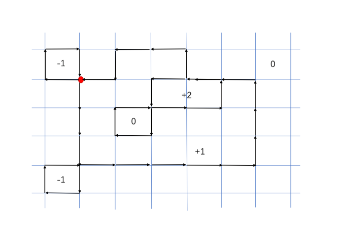
Figure 1. A closed walk of length ${{N}}=36$ starting from and returning to the same bullet red point with its various winding sectors $m=+2,+1,0,-1,-1$ (containing respectively $2,14,1,1,1$ unit lattice cells). Note the double arrow on the horizontal link (above the +2 sector) which indicates that the walk has moved twice on this link, here in the same left direction.

In Figure 1, the $0$-winding sector inside the walk arises from a superposition of a $+1$ and a $-1$ winding. Summing the areas of each sector, with the corresponding multiplicative weight, gives the signed area $A={(-1)}\times{2}+(+0)\times 1+{(+1)}\times{14}+{(+2)}\times{2}=16.$

More formally, if $\gamma:[0,1]\rightarrow\mathbb{R}^{2}$ is a closed path that begins and ends at the origin, the signed area of this path is

$$A=\int_{\mathbb{R}^{2}}\eta(\gamma,\mathbf{x})d\mathbf{x}=\sum_{m=-\infty}^{\infty}mS_{m},$$ (1)

where $\eta(\gamma,\mathbf{x})$ is the winding number of $\gamma$ around the point $\mathbf{x}\in\mathbb{R}^{2}$, and where $S_{m}$ denotes the classical area of the $m$-winding sectors inside the path (i.e. the number of unit lattice cells it encloses with winding number $m$, where $m$ can be positive or negative).

Winding sectors for continuous Brownian curves as well as for discrete lattice walks have been the subject of study for a long time. In this respect, we note in the last few years some advances in [2] where an explicit formula for the expected area $\langle S_{m}\rangle$ of the $m$-winding sectors inside square-lattice walks is proposed, to the exception of the $0$-winding sector, for the simple reason that the latter is difficult to distinguish from the outside (i.e. $0$-winding again) sector, which is of infinite size. Taking the continuous limit allows us to recover the results previously obtained in [4] for Brownian curves. One notes that for Brownian curves the expected area $\langle S_{0}\rangle$ of the $0$-winding sectors is also known by other means thanks to the SLE machinery [7]. However, it remains an open problem for discrete lattice walks.

Counting the number of closed walks of length ${N}$ on the square lattice enclosing a signed area $A$ can be achieved in a most straightforward way by introducing two lattice hopping operators (symbols) $u$ and $v$ respectively in the right and up directions, as well as operators $u^{-1}$ and $v^{-1}$ corresponding to hops in the left and down direction. A directed walk on the square lattice starting at the origin is then represented by the ordered product of the hopping operators corresponding to its individual steps. By convention we order the operators from right to left as we trace the steps of the walk: $vu$ corresponds to a up step $u$, followed by a right step $v$. Clearly the set of all walks of length ${N}$ on the lattice is reproduced by the $4^{{N}}$ terms in the expansion of

$$\big{(}u+u^{-1}+v+v^{-1}\big{)}^{{N}}$$ (2)

into monomials of products of symbols, each with ${N}$ factors. The operator $u+u^{-1}+v+v^{-1}$ can be considered as the generator of walks.

We are interested in closed walks, and in counting their multiplicity according to their signed area. To this end, we endow the above operators with the relations

$$uu^{-1}=u^{-1}u=vv^{-1}=v^{-1}v=1,$$ (3)

to which we add a non-commutativity relation (which expresses the fact that the elementary walk circling one lattice cell in the counterclockwise direction has signed area $1$):

$$v^{-1}\;u^{-1}\;v\;u=\mathrm{Q},$$ (4)

where $\mathrm{Q}$ is a central element (that is, $\mathrm{Q}$ commutes with all operators). This entails

$$vu=\mathrm{Q}uv,\quad vu^{-1}=\mathrm{Q}^{-1}u^{-1}v,\quad v^{-1}u=\mathrm{Q}^{-1}uv^{-1},\quad v^{-1}u^{-1}=\mathrm{Q}u^{-1}v^{-1},$$ (5)

which allows us to reduce all terms in (2) into monomials of the form $u^{m}v^{n}$, $(m,n)\in{\mathbb{Z}}^{2}$ being the lattice coordinates of the end of the walk, with coefficients which are powers of $\mathrm{Q}$. In particular, closed walks correspond to the monomial $u^{0}v^{0}$ in (2).

The non-commutativity relation $vu=\mathrm{Q}\;uv$ has the effect of flipping a right-up two-step segment into an up-right one, producing a factor of $\mathrm{Q}$, and similarly for each relation in (5). In each case, the coefficient is $\mathrm{Q}$ to the power of the signed area of the unit lattice cells left behind by the exchange. Repeated application of these relations reduces each walk to hook-shape walk $u^{m}v^{n}$ with an overall coefficient $\mathrm{Q}^{A}$, with $A$ the signed area of the original walk prolonged into a closed walk by joining its end to the origin with a vertical and a horizontal straight walk. In particular, closed walks correspond to monomials $\mathrm{Q}^{A}u^{0}v^{0}$, with $A$ the signed area of the walk. This area is maximal if the walk forms a square of width $N/4$, and then the signed area is $\pm N^{2}/16$. Therefore, using the notation $[u^{0}v^{0}]$ for the extraction of the constant term in a Laurent polynomial in $u$ and $v$, the distribution of the signed area of closed walks of length $N$ is given by

$$[u^{0}v^{0}]\big{(}u+u^{-1}+v+v^{-1}\big{)}^{{N}}={\sum_{A=-\lfloor N^{2}/16\rfloor}^{\lfloor N^{2}/16\rfloor}C_{{N}}(A)\;\mathrm{Q}^{A}},$$ (6)

where $C_{{N}}(A)$ counts the closed walks of length ${N}$ enclosing a signed area $A$. For example, one easily checks that $[u^{0}v^{0}]\big{(}u+u^{-1}+v+v^{-1}\big{)}^{4}=28+4\mathrm{Q}+4\mathrm{Q}^{-1}$, indicating that among the $\binom{4}{2}^{2}=36$ closed walks making $4$ steps $C_{4}(0)=28$ enclose a signed area $A=0$ and $C_{4}(1)=C_{4}(-1)=4$ enclose a signed area $A=\pm 1$.

2. The Hofstadter model

In any irreducible representation of the operator relation $vu=Quv$, the central element $\mathrm{Q}$ will be represented by a number. Restricting to unitary representations, for which $u^{\dagger}=u^{-1}$, $v^{\dagger}=v^{-1}$, $\mathrm{Q}$ will necessarily be a complex number of norm unity, i.e., a phase. This provides a mapping between the $u,v$ representation for walks and quantum mechanics, interpreting $u$ and $v$ as unitary operators acting on a quantum Hilbert space, and the operator $u+u^{-1}+v+v^{-1}$ as the Hamiltonian of a quantum system.

In fact, such a quantum system exists and corresponds to a well-known model in physics. Interpreting $u$ and $v$ as operators that generate hops of a quantum particle by one link on the square lattice, the non-commutativity relation $vu=Quv$ indicates that translations of the particle in the horizontal and vertical directions do not commute. This can be interpreted as that the particle is charged and coupled to a homogeneous magnetic field perpendicular to the lattice. The magnetic flux associated to this (constant) vector field is $\Phi a^{2}$ for any surface of area $a^{2}$.

Let us now take $\mathrm{Q}={\mathrm{e}}^{{\mathrm{i}}2\pi\Phi/\Phi_{o}}$, where $\Phi$ is the magnetic flux through any unit lattice cell (i.e. for the surface of the square of width $a=1$) and where $\Phi_{o}=h/c$ is the flux quantum ($h$ is the Planck constant and $c$ the particle’s charge). The Hermitian operator

$$H=u+u^{-1}+v+v^{-1}$$ (7)

then becomes a Hamiltonian modelling a quantum particle hopping on a square lattice and coupled to a perpendicular magnetic field. This model is known as the Hofstadter model [8].

To make the physics connection completely explicit, we note that in quantum mechanics the hopping operators $u$ and $v$ are written as

$$u=\mathrm{e}^{\mathrm{i}(p_{x}-cA_{x})/\hbar}\text{\quad and \quad}v=\mathrm{e}^{\mathrm{i}(p_{y}-cA_{y})/\hbar},$$

where $A_{x}=-\Phi y$  and $A_{y}=0$ are the two components of the vector potential of the magnetic field in the Landau gauge and $p_{x}=-\mathrm{i}\hbar{\partial_{x}}$ and $p_{y}=-\mathrm{i}\hbar{\partial_{y}}$ those of the momentum operator (where we use the standard notation $\hbar=h/(2\pi)$). Thus, assuming (2), the relation $vu=Quv$ follows from the Baker–Campbell–Hausdorff formula, using the Heisenberg commutators $[x,p_{x}]=[y,p_{y}]=\mathrm{i}\hbar$ (this identity is often called the “canonical commutation relation”).

One now introduces the quantum state $\Psi_{m,n}$ representing the probability amplitude of the particle being at lattice site $(m,n)$, on which hopping operators act as

$$u\Psi_{m,n}={\mathrm{e}}^{{\mathrm{i}}cn\Phi/\hbar}\Psi_{m+1,n}~{},\quad v\Psi_{m,n}=\Psi_{m,n+1}.$$

As $c\Phi/\hbar$ = $2\pi\Phi/(h/c)=2\pi\Phi/\Phi_{o}$, the factor appearing in the action of $u$ on $\psi_{m,n}$ is $\mathrm{Q}^{n}$. Using translation invariance in the horizontal direction we can further choose $\Psi_{m,n}$ to be an eigenstate of $p_{x}$, that is, $\Psi_{m,n}={\mathrm{e}}^{{\mathrm{i}}mk_{x}}\Phi_{n}$. The action of $u,v$ on $\Phi_{n}$ becomes

$$u\Phi_{n}={\mathrm{e}}^{{\mathrm{i}}k_{x}}\mathrm{Q}^{n}\Phi_{n}~{},~{}~{}~{}v\Phi_{n}=\Phi_{n+1}.$$

For the Hofstadter model, the Schrödinger equation $H\Psi=E\Psi$ (which determines the eigenvalue $E$ of the spectrum) can be rewritten as

$$(u+u^{-1}+v+v^{-1})\Psi_{m,n}=E\Psi_{m,n}\Rightarrow\Phi_{n+1}+\Phi_{n-1}+(\mathrm{Q}^{n}{\mathrm{e}}^{{\mathrm{i}}k_{x}}+\mathrm{Q}^{-n}{\mathrm{e}}^{-{\mathrm{i}}k_{x}})\Phi_{n}=E\Phi_{n}.$$

Going a step further, a simplification arises when the flux is rational (i.e. when one has $\mathrm{Q}=\mathrm{e}^{\mathrm{i}2\pi p/q}$ with $p,q$ two coprime integers): It induces a $q$-periodicity of the Schrödinger equation in the vertical direction. Then, as Bloch’s theorem states that solutions to the Schrödinger equation in a periodic potential take the form of a plane wave modulated by a periodic function ${\tilde{\Phi}}_{n}$, we can write

$$\Phi_{n}={\mathrm{e}}^{{\mathrm{i}}nk_{y}}{\tilde{\Phi}}_{n}~{},~{}~{}~{}{\tilde{\Phi}}_{n+q}={\tilde{\Phi}}_{n}.$$ (8)

Indeed, for this rational flux $\mathrm{Q}^{q}=1$, thus $u^{q},v^{q}$ become Casimirs (a physicist’s term for central elements), and the choice of Bloch states (8) can be interpreted mathematically as choosing an irreducible representation of the $u,v$ algebra. Acting on such states, $u^{q}$ and $v^{q}$ become $u^{q}={\mathrm{e}}^{{\mathrm{i}}qk_{x}}$ and $v^{q}=\mathrm{e}^{{\mathrm{i}}qk_{y}}$. One ends up with $u$ and $v$, acting on ${\tilde{\Phi}}_{n}$, becoming the $q\times q$ matrices

$$u=\mathrm{e}^{\mathrm{i}k_{x}}\begin{pmatrix}\mathrm{Q}\quad&0&0&\cdots&0&0\\ 0\quad&\mathrm{Q}^{2}&\quad 0\quad&\cdots&0&0\\ 0\quad&0&\mathrm{Q}^{3}&\cdots&0&0\\ \vdots&\vdots&\vdots&\ddots&\vdots&\vdots\\ 0\quad&0&0&\cdots&\mathrm{Q}^{q-1}&0\\ 0\quad&0&0&\cdots&\quad 0\quad&1\\ \end{pmatrix}\text{\quad and \quad}v=\mathrm{e}^{\mathrm{i}k_{y}}\begin{pmatrix}0\quad&1&0&\cdots&0&0\\ 0\quad&0&\quad 1\quad&\cdots&0&0\\ 0\quad&0&0&\cdots&0&0\\ \vdots&\vdots&\vdots&\ddots&\vdots&\vdots\\ 0\quad&0&0&\cdots&0&1\\ 1\quad&0&0&\cdots&\quad 0\quad&0\\ \end{pmatrix}$$

involving two real quantities $k_{x}$ and $k_{y}$. Finding the energy spectrum (which depends on $k_{x}$and $k_{y}$) reduces to computing the eigenvalues $E_{1},\ldots,E_{q}$ of the $q\times q$ Hamiltonian matrix $H_{q}:=u+u^{-1}+v+v^{-1}$, i.e.

$$H_{q}=\begin{pmatrix}\mathrm{Q}{\mathrm{e}}^{{\mathrm{i}}k_{x}}+\mathrm{Q}^{-1}{\mathrm{e}}^{-{\mathrm{i}}k_{x}}&{\mathrm{e}}^{{\mathrm{i}}k_{y}}&0&\cdots&0&{\mathrm{e}}^{-{\mathrm{i}}k_{y}}\\ {\mathrm{e}}^{-{\mathrm{i}}k_{y}}&\mathrm{Q}^{2}{\mathrm{e}}^{{\mathrm{i}}k_{x}}+\mathrm{Q}^{-2}{{\mathrm{e}}^{-{\mathrm{i}}k_{x}}}&\quad{\mathrm{e}}^{{\mathrm{i}}k_{y}}\quad&\cdots&0&0\\ 0&{\mathrm{e}}^{-{\mathrm{i}}k_{y}}&()&\cdots&0&0\\ \vdots&\vdots&\vdots&\ddots&\vdots&\vdots\\ 0&0&0&\cdots&()&{\mathrm{e}}^{{\mathrm{i}}k_{y}}\\ {\mathrm{e}}^{{\mathrm{i}}k_{y}}&0&0&\cdots&\quad{\mathrm{e}}^{-{\mathrm{i}}k_{y}}\quad&\mathrm{Q}^{q}{\mathrm{e}}^{{\mathrm{i}}k_{x}}+\mathrm{Q}^{-q}{{\mathrm{e}}^{-{\mathrm{i}}k_{x}}}\\ \end{pmatrix}.$$

All the machinery of quantum mechanics is now at our disposal. Selecting as in (6) the $u^{0}v^{0}$ monomial of $\big{(}u+u^{-1}+v+v^{-1}\big{)}^{{N}}$ translates in the quantum world to computing the trace of $H_{q}^{{{N}}}$. The quantum trace is defined as

$$\textbf{Tr}\,H_{q}^{{N}}{:=\frac{1}{q}\int_{-\pi}^{\pi}\int_{-\pi}^{\pi}\frac{dk_{x}}{2\pi}\frac{dk_{y}}{2\pi}\;{\rm tr}\,H_{q}^{{N}}}=\frac{1}{q}\int_{-\pi}^{\pi}\int_{-\pi}^{\pi}\frac{dk_{x}}{2\pi}\frac{dk_{y}}{2\pi}\sum_{i=1}^{q}E_{i}^{{N}},$$ (9)

that is, one sums over the $q$ eigenvalues $E_{i}$ of $H_{q}$ (yielding the standard matrix trace ${\rm tr}\,H_{q}^{{N}}$) and integrates over $k_{x}$ and $k_{y}$ while enforcing a continuous normalization in $k_{x},k_{y}$ and one rescales by a factor $1/q$ (thus, if one considers for example the $q\times q$ identity matrix $I_{q}$, one has ${\rm tr}\,I_{q}=q$, while $\textbf{Tr}\,I_{q}=1$). Under this definition of the trace, $\textbf{Tr}\,u^{m}v^{n}=\delta_{m,0}\delta_{n,0}$ (integration over $k_{x},k_{y}$ eliminates the traces of terms involving $u^{qm}$ and $v^{qn}$). We thus get a first noteworthy result (also obtained via another approach by Bellisard et al. in [1]):

Theorem 2.1.

Assuming $q>\frac{N^{2}}{8}$, the signed area enumeration of closed paths is given by

$$\sum_{A}C_{{N}}(A)\;\mathrm{Q}^{A}={\textbf{Tr}}\;H_{q}^{{{N}}}.$$ (10)

3. The signed area enumeration

It is known (see e.g. William Chambers’ book [3]) that the determinant of the matrix $I_{q}-zH_{q}$ satisfies

$$\det(I_{q}-zH_{q})=\left(\sum_{n=0}^{\lfloor q/2\rfloor}(-1)^{n}Z(n)z^{2n}\right)-2\big{(}\cos(qk_{x})+\cos(qk_{y})\big{)}z^{q},$$

where the $Z(n)$’s are independent of $k_{x}$ and $k_{y}$ and $Z(0)=1$. Christian Kreft [12] was able to rewrite $Z(n)$ in a closed form as trigonometric multiple nested sums

$$Z(n)=\sum_{k_{1}=1}^{q-2n+2}\sum_{k_{2}=1}^{k_{1}}\cdots\sum_{k_{n}=1}^{k_{n-1}}\prod_{j=1}^{n}s_{k_{j}+2n-2j},$$ (11)

where

$$s_{k}=4\sin^{2}(\pi kp/q)=2-Q^{k}-Q^{-k}.$$ (12)

We call $s_{k}$ the spectral function of the model. This is the starting point for the signed area enumeration. We give here a summary of the procedure, more details can be found in [16, 14]. First introduce the coefficients $b(n)$ via

$$-\log\left(\sum_{n=0}^{\lfloor q/2\rfloor}(-1)^{n}Z(n)z^{2n}\right)=\sum_{n=1}^{\infty}b(n)z^{2n}.$$ (13)

The $b(n)$ are related to the desired traces. Start by noting that

$$\textbf{Tr}\;H_{q}^{2n}=\frac{1}{q}{\rm tr}\,H_{q}^{2n}~{}~{}~{}\text{for}~{}~{}~{}n<q.$$

Indeed, one has ${\rm tr}\,u^{i}v^{j}=q\;\delta_{i,0}\delta_{j,0}$ for $i,j<q$ and so the values of the Casimirs $k_{x},k_{y}$ do not appear, making the integration over them in (9) trivial. Then the identity

$$-\log\,\det(I_{q}-zH_{q})=-{\rm tr}\,\log(I_{q}-zH_{q})=\sum_{n=1}^{\infty}\frac{z^{n}}{n}{\rm tr}\,H_{q}^{n}=\sum_{n=1}^{\lfloor q/2\rfloor}b(n)z^{2n}+O(z^{q})$$

implies that the quantum trace (9) is proportional to $b(n)$ for $n<q$

$$\textbf{ Tr}\,H_{q}^{2n}=\frac{2n}{q}b(n).$$

Now, by keeping $q$ as a free parameter and extending it to arbitrarily big values, the quantum trace can be calculated for all $n$.

Note that the term of order $z^{n}$ in $\det(I_{q}-zH_{q})$ is $-(z^{n}/n){\rm tr}\,H_{q}^{n}$ plus terms involving products of traces, ${\rm tr}\,H_{q}^{n_{1}}\,{\rm tr}\,H_{q}^{n_{2}}\cdots$ with $n_{1}+n_{2}+\cdots=n$. As each trace ${\rm tr}\,H_{q}^{n_{i}}$ contributes an overall factor $q$, $b(n)$ can also be obtained as the order $q$ term in $Z(n)$, ignoring terms of higher order $q^{2},\dots,q^{n}$. Since each sum in Formula (11) contributes a factor of $q$, we get the following explicit expression for $b(n)$:

$$b(n)=\sum_{j=1}^{n}{\sum_{\begin{subarray}{c}l_{1},l_{2},\ldots,l_{j}\\ {\rm composition}\;{\rm of}\;n\end{subarray}}\hskip-11.38092pt{c(l_{1},l_{2},\ldots,l_{j})}}{\sum_{k=1}^{q-j+1}s^{l_{j}}_{k+j-1}\cdots s^{l_{2}}_{k+1}{s}^{l_{1}}_{k}},$$ (14)

$$\text{where\ }c(l_{1},l_{2},\ldots,l_{j}):=\frac{\binom{l_{1}+l_{2}}{l_{1}}}{l_{1}+l_{2}}\;\;l_{2}\frac{\binom{l_{2}+l_{3}}{l_{2}}}{l_{2}+l_{3}}\;\cdots\;\;l_{{j}-1}\frac{\binom{l_{{j}-1}+l_{j}}{l_{{j}-1}}}{l_{{j}-1}+l_{j}}.$$

Here, the coefficients $c(l_{1},l_{2},\ldots,l_{j})$ are labelled by the compositions $l_{1},l_{2},\ldots,l_{j}$ of $n$, i.e. the ordered partitions of $n$ (thus, there are $2^{n-1}$ compositions of $n$, for example $3=3,2+1,1+2,1+1+1$). Note that the expression for $c(l_{1},l_{2},\ldots,l_{j})$ is closely related to the enumeration of Dyck paths (up to a factor $l_{1}$); see Christian Krattenthaler’s article [11, p. 516]. We have further elaborated on this relation in [6].

Putting everything together, we get

$$\textbf{ Tr}\;H_{q}^{2n}=\sum_{j=1}^{n}{\sum_{\begin{subarray}{c}l_{1},l_{2},\ldots,l_{j}\\ {\rm composition}\;{\rm of}\;n\end{subarray}}\hskip-11.38092pt{c(l_{1},l_{2},\ldots,l_{j})}}\;\frac{2n}{q}\ \ {\sum_{k=1}^{q-j+1}s^{l_{j}}_{k+j-1}\cdots s^{l_{2}}_{k+1}{s}^{l_{1}}_{k}}.$$

What is more, the trigonometric sums involved in this formula can be computed, keeping $q$ as a free parameter. Finally, returning to (10) (with $N=2n$) the desired number of closed walks of given area is given by the following theorem.

Theorem 3.1.

The number of closed walks of length $2n$ enclosing a given signed area $A$ is

$$C_{2n}(A) =\ 2n\times\sum_{j=1}^{n}{\sum_{\begin{subarray}{c}l_{1},l_{2},\ldots,l_{j}\\ \text{ composition of}\;n\end{subarray}}{\frac{\binom{l_{1}+l_{2}}{l_{1}}}{l_{1}+l_{2}}\;\;l_{2}\frac{\binom{l_{2}+l_{3}}{l_{2}}}{l_{2}+l_{3}}\;\cdots\;\;l_{{j}-1}\frac{\binom{l_{{j}-1}+l_{j}}{l_{{j}-1}}}{l_{{j}-1}+l_{j}}}}~{}\times$$

$$\hskip-45.52458pt{\sum_{k_{3}=0}^{2l_{3}}\sum_{k_{4}=0}^{2l_{4}}\ldots\sum_{k_{j}=0}^{2l_{j}}\prod_{i=3}^{j}\binom{2l_{i}}{k_{i}}}{\binom{2l_{1}}{l_{1}+A+\sum_{i=3}^{j}(i-2)(k_{i}-l_{i})}\binom{2l_{2}}{l_{2}-A-\sum_{i=3}^{j}(i-1)(k_{i}-l_{i})}}.$$

This formula grows quickly in complexity since one has to sum over $2^{n}-1$ compositions. Its complexity is analysed in more detail in the following proposition.

Proposition 3.2.

The formula for $C_{2n}(A)$ in Theorem 3.1 involves asymptotically, up to some polynomial factor, $(4/(5-\sqrt{17}))^{n}\approx 4.56^{n}$ summands.

Proof 3.3.

This number of summands is given by

$$r(n):=\sum_{j=1}^{n}\sum_{\begin{subarray}{c}l_{1},l_{2},\ldots,l_{j}\\ \text{ composition of}\;n\end{subarray}}(2l_{3}+1)(2l_{4}+1)\dotsm(2l_{j}+1).$$

The sequence starts like $(r(n))_{n\geq 1}=(1,2,6,24,106,480,2186,9968,45466,\dots)$. Thus, $r(n)$ counts compositions of $n$ where each summand $l_{i}$ (for $i\geq 3$) can have $2l_{i}+1$ colours. Let us consider first compositions of $n$ where each summand $l_{i}$ (for $i\geq 1$) can have $2l_{i}+1$ colours; their generating function is

$$S(z)=\frac{1}{1-\sum_{i\geq 1}(2i+1)z^{i}}=\frac{\left(z-1\right)^{2}}{2z^{2}-5z+1}.$$

This corresponds to the sequence $\oeis{A060801}$ in the On-line Encyclopedia of Integer Sequences. In our case, the $i\geq 3$ constraint modifies a little bit the generating function and one has to sum the compositions having 1 or 2 parts and those having 3 parts or more; one gets the following generating function

$$R(z) =\sum_{n\geq 1}r_{n}z^{n}=\frac{z}{1-z}+\left(\frac{z}{1-z}\right)^{2}+\left(\frac{z}{1-z}\right)^{2}(S(z)-1)$$

$$=\frac{z^{2}-4z+1}{2z^{2}-5z+1}\frac{z}{1-z}.$$

It entails $r(n)=5r(n-1)-2r(n-2)-2$ (with $r(1)=1$ and $r(2)=2$); accordingly, $r(n)$ grows like $\phi^{n}$ with $\phi=4/(5-\sqrt{17})$, which is coherent with the fact that $1/\phi$ is the dominant pole of $R(z)$. In conclusion, our formula for $C_{2n}(A)$ involves in total asymptotically $\phi^{n}\approx 4.56^{n}$ summands (each leading additionally to a polynomial cost in $n$ for the product of all the binomials), which is still much less than the naive generation of all $\binom{2n}{n}^{2}$ closed walks of length $2n$, which would be of cost $>16^{n}/(\pi n)$.

Note that it is in fact possible to compute $C_{2n}$ in polynomial time: Using the non-commutative relations (5), the expansion of $(u+v+u^{-1}+v^{-1})^{2n}$ simplifies a lot and in fact has $O(n^{4})$ monomials $u^{i}v^{j}Q^{k}$. This gives an algorithm of complexity $O(n^{6})$ to compute $C_{2n}(A)$. Thus, our formula (of exponential cost) in Theorem 3.1 is not the fastest way to compute $C_{2n}(A)$, but it has the benefit of being the first explicit formula (as far as we are aware of!).

Let us end this section with a probabilistic remark. In the limit of the elementary lattice size $a\to 0$ and the walk length $2n\to\infty$ with the scaling $na^{2}=t$, walks converge to Brownian motion curves and we recover the continuum limit of a particle moving on the plane in a constant magnetic field. To implement this limit, we rescale the lattice cell area to $a^{2}$, which amounts to setting $A\to A/a^{2}$ in $C_{2n}(A)$. Numerical simulations then suggest the following conjecture.

Conjecture 3.4.

The signed area of closed walks of length $2n$ converges, after rescaling, to the following distribution (for any $\alpha>0$)

$$\frac{2n\;C_{2n}(\alpha n)}{\binom{2n}{n}^{2}}\to\frac{\pi}{\cosh^{2}(\alpha\pi)}.$$

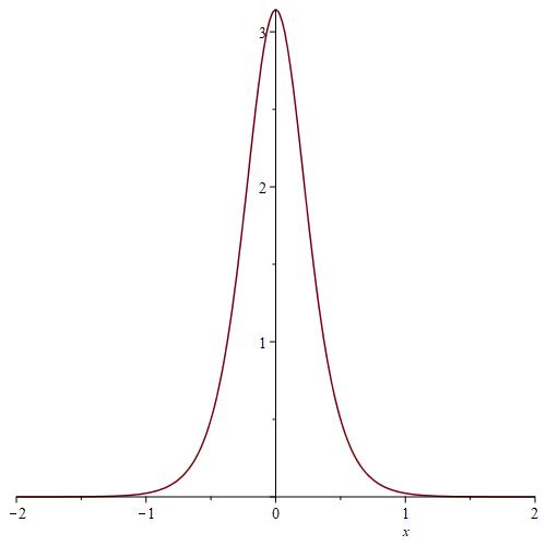
Figure 2. We conjecture that the distribution of the signed area asymptotically follows…not a Gaussian limit law (as it may be thought at first glance), but the $1/\cosh^{2}$ distribution of Paul Lévy. For small values of $A$, and $n$ up to $70$, we checked numerically that the convergence gets better when $n$ increases.

This conjecture is consistent with the law for the distribution of the signed area enclosed by a Brownian curve after a time $t$ (obtained by Paul Lévy in 1950; see [13, 10]). It can also be obtained directly in the continuum limit by considering the partition function of a quantum particle in a magnetic field with a Landau level energy spectrum.

4. Exclusion statistics

The quantities $Z(n)$ and $b(n)$ introduced previously admit a statistical mechanical interpretation. Let us write the spectral function $s_{k}$ in (12) as $s_{k}={\mathrm{e}}^{-\beta\epsilon_{k}}$ ($\beta$ is the inverse temperature) and interpret is as the Boltzmann factor for a quantum 1-body spectrum $\epsilon_{k}$ labelled by an integer $k$. The structure of $Z(n)$ in (11) then precisely corresponds to an $n$-body partition function for a gas of particles with 1-body spectrum $\epsilon_{k}$ and exclusion statistics $g=2$: The $+2$ shifts in the spectral function arguments ensure that no two particles can occupy adjacent quantum states. Exclusion statistics is, again, a purely quantum concept which describes the statistical mechanical properties of identical particles. Ordinary particles are either bosons ($g=0$), which can occupy the same quantum state, or fermions ($g=1$), which cannot occupy the same quantum state. We see that square-lattice walks map to systems with statistics beyond Fermi exclusion, in which particles can occupy neither the same state nor adjacent states. In a sense, each particle excludes two quantum states, thus $g=2$. In general, for $g$-exclusion particles the $n$-body partition function (11) would become

$$Z(n)=\sum_{k_{1}=1}^{q-gn+g}\sum_{k_{2}=1}^{k_{1}}\cdots\sum_{k_{n}=1}^{k_{n-1}}s_{k_{1}+gn-g}s_{k_{2}+gn-2g}\cdots s_{k_{n-1}+g}s_{k_{n}},$$ (15)

where one observes a shift $g$ instead of $2$ in the arguments of the spectral function. In line with (13), (14) the associated $n$-th cluster coefficient can be shown to take the form

$$b(n)=\sum_{j=1}^{n}\sum_{\begin{subarray}{c}l_{1},l_{2},\ldots,l_{j}\\ {g-{\rm composition}\;{\rm of}\;n}\end{subarray}}\hskip-11.38092pt{c_{g}(l_{1},l_{2},\ldots,l_{j})}{\sum_{k=1}^{q-j+1}s^{l_{j}}_{k+j-1}\cdots s^{l_{2}}_{k+1}{s}^{l_{1}}_{k}},$$ (16)

where

$${c_{g}(l_{1},l_{2},\ldots,l_{j})}:={{{\frac{(l_{1}+\dots+l_{g-1}-1)!}{l_{1}!\cdots l_{g-1}!}}~{}\prod_{i=1}^{j-g+1}\binom{l_{i}+\dots+l_{i+g-1}-1}{l_{i+g-1}}}}.$$

In (16) one sums over all $g$-compositions of the integer $n$, obtained by inserting at will inside the usual compositions (i.e., the $2$-compositions) no more than $g-2$ zeroes in succession. For example, for $n=3$ and $g=3$ one has $9$ such $3$-compositions:

$$3,2+1,1+2,1+1+1,2+0+1,1+0+2,1+0+1+1,1+1+0+1,1+0+1+0+1.$$

For general $g$ there are $g^{n-1}$ such $g$-compositions of the integer $n$ (see [9] for an analysis of these extended compositions, also called multicompositions).

One has reached the conclusion that the signed area enumeration for walks on the square lattice is described by a quantum gas of particles with statistical exclusion $g=2$. To relate this explicitly to properties of the Hofstadter Hamiltonian itself, let us perform on the hopping lattice operators $u$ and $v$ the transformation

$$u\to-u\;v,~{}~{}~{}v\to v,$$

which leave their own commutation relation invariant to get the new Hamiltonian

$$H=-u\;v-v^{-1}u^{-1}+v+v^{-1}$$ (17)

still describing the same walks but on a deformed lattice.

This new Hamiltonian (if one compares it with the initial Hamiltonian operator (7) of the Hofstadter model) has the advantage to lead to simpler matrix

$$I_{q}-zH_{q}=\begin{pmatrix}{1}&-{(1-\mathrm{Q})}z&0&\cdots&0&0\\ -{(1-{\frac{1}{\mathrm{Q}}})}z&{1}&-{(1-\mathrm{Q}^{2})}z&\cdots&0&0\\ 0&-(1-{\frac{1}{\mathrm{Q}^{2}}})z&{1}&\cdots&0&0\\ \vdots&\vdots&\vdots&\ddots&\vdots&\vdots\\ 0&0&0&\cdots&{1}&-{(1-{\mathrm{Q}^{q-1}})}z\\ 0&0&0&\cdots&-{(1-{\frac{1}{\mathrm{Q}^{q-1}}})}z&{1}\\ \end{pmatrix},$$ (18)

where we set $k_{x}=k_{y}=0$ for simplicity (since, as we explained in Section 3, $k_{x}$ and $k_{y}$ do not appear in the counting formula). The Hofstadter spectral function (12) becomes

$$s_{k}=(1-\mathrm{Q}^{k})(1-{\frac{1}{\mathrm{Q}^{k}}}).$$

The matrix (18) is a particular case of the more general class of matrices having the following shape

$$I_{q}-zH_{q}=\begin{pmatrix}{1}&-{f(1)}z&{0}&\cdots&0&-{g(q)}z\\ -{g(1)}z&{1}&-{f(2)}z&\cdots&0&0\\ 0&-{g(2)}z&{1}&\cdots&0&0\\ \vdots&\vdots&\vdots&{\ddots}&\vdots&\vdots\\ 0&0&0&\cdots&{1}&-{f(q-1)}z\\ -{f(q)}z&0&0&\cdots&-{g(q-1)}z&{1}\\ \end{pmatrix}$$ (19)

and associated spectral functions

$${s_{k}=f(k)g(k)},$$

which become the building blocks of the $Z(n)$’s in (11) (up to spurious “umklapp” terms, a name deriving from momentum periodicity effects on lattice quantum models, which disappear if $f(q)$ and $g(q)$ both vanish).

For statistics $g=3$, the matrix (19) generalizes in a natural way to

$$\hskip 5.69054ptI_{q}-zH_{q}=\begin{pmatrix}{1}&-{f(1)}z&0&0&\cdots&0&-{g(q-1)}z&{0}\\ {0}&{1}&-{f(2)}z&0&\cdots&0&0&-{g(q)}z\\ -{g(1)}z&{0}&{1}&-{f(3)}z&\cdots&0&0&0\\ 0&-{g(2)}z&{0}&{1}&\cdots&0&0&0\\ \vdots&\vdots&\vdots&\vdots&{\ddots}&\vdots&\vdots&\vdots\\ 0&0&0&0&\cdots&{1}&-{f(q-2)}z&0\\ 0&0&0&0&\cdots&{0}&{1}&-{f(q-1)}z\\ -{f(q)}z&0&0&0&\cdots&-{g(q-2)}z&{0}&{1}\\ \end{pmatrix},$$ (20)

that is, with an extra vanishing paradiagonal below the unity main diagonal, which is the manifestation of the stronger $g=3$ exclusion.

The spectral function corresponding to this matrix is

$$s_{k}=g(k)f(k)f(k+1)$$

and the determinant $\det(I_{q}-zH_{q})$ assumes the form (15) with $g=3$. For $g$-exclusion the generalization of  (20) amounts to a Hamiltonian of the form

$$H=F(u)v+v^{{1-g}}G(u),$$ (21)

and $I-zH$ is then a matrix with $g-2$ vanishing paradiagonals below the main diagonal (here $q$ is left arbitrary but always understood to be larger than $g$). The spectral parameters of this matrix are

$$F(\mathrm{Q}^{k})=f(k),\quad G(\mathrm{Q}^{k})=g(k),$$

and the spectral function is

$${s_{k}=g(k)f(k)f(k+1)\ldots f(k+g-2)}.$$

Clearly the Hofstadter Hamiltonian (17), which rewrites as $H=(1-u)v+v^{{1-2}}(1-u^{-1})$, is a particular case of (21) with $g=2$ and $F(u)=1-u$, $G(u)=1-u^{-1}$.

5. Chiral walks on the triangular lattice

Let us illustrate this mechanism in the case of $g=3$ exclusion with the specific example of chiral walks on a triangular lattice. The three hopping operators $U,V$ and $W=\mathrm{Q}U^{-1}V^{-1}$ described in Figure 3 are such that $VU=\mathrm{Q}^{2}UV$.

Figure 3. The three hopping operators $U,V$ and $W$ on the triangular lattice.

The triangular lattice Hamiltonian is

$$H=U+V+W.$$

It generates walks composed of triangles either pointing up and winding in the counterclockwise direction, or pointing down and winding in the negative direction. In this sense, the walks are chiral. The factor $\mathrm{Q}$ in the definition of $W$ and the factor $\mathrm{Q}^{2}$ in the commutation of $U,V$ are chosen so that up-pointing (positive) triangles are assigned area $+1$. Figure 4 depicts some examples of chiral walks on the triangular lattice.

Figure 4. Examples of closed chiral walks on the triangular lattice.

To bring $H$ to the exclusion form (21) one chooses the representation $U=-{\mathrm{i}}\,u\,v$ and $V={\mathrm{i}}\,u^{-1}\,v$, with $u$ and $v$ as before, in which case $H$ rewrites as

$$H={\mathrm{i}}(-u+u^{-1})v+v^{-2}.$$

In this form, $H$ is indeed a Hamiltonian of the type (21) for $g=3$ exclusion, with $F(u)={\mathrm{i}}(-u+u^{-1})$, $G(u)=1$, spectral parameters

$$f(k)=-{\mathrm{i}}(\mathrm{Q}^{k}-\frac{1}{\mathrm{Q}^{k}}),\quad g(k)=1,$$

spectral function

$$s_{k}=g(k)f(k)f(k+1)=4\sin(2\pi pk/q)\sin\big{(}2\pi p(k+1)/q\big{)},$$ (22)

and matrix

$$I_{q}-zH_{q}=\begin{pmatrix}{1}&\mathrm{i}(\mathrm{Q}-{\frac{1}{\mathrm{Q}}})z&0&0&\cdots&0&-z&{0}\\ {0}&{1}&\mathrm{i}(\mathrm{Q}^{2}-{\frac{1}{\mathrm{Q}^{2}}})z&0&\cdots&0&0&-z\\ -z&{0}&{1}&\mathrm{i}(\mathrm{Q}^{3}-\frac{1}{\mathrm{Q}^{3}})z&\cdots&0&0&0\\ 0&-z&{0}&{1}&\cdots&0&0&0\\ \vdots&\vdots&\vdots&\vdots&{\ddots}&\vdots&\vdots&\vdots\\ 0&0&0&0&\cdots&{1}&\mathrm{i}(\mathrm{Q}^{q-2}-{\frac{1}{\mathrm{Q}^{q-2}}})z&0\\ 0&0&0&0&\cdots&{0}&{1}&\mathrm{i}(\mathrm{Q}^{q-1}-{\frac{1}{\mathrm{Q}^{q-1}}})z\\ 0&0&0&0&\cdots&-z&{0}&{1}\\ \end{pmatrix},$$

which is of the type (20) with a vanishing bottom-left entry. The non-Hermiticity of the triangular Hamiltonian, and thus of $I_{q}-zH_{q}$, is a consequence of the chiral nature of the walks.

The triangular signed area enumeration follows [14], yielding an expression similar to Theorem 3.1 with the trigonometric single sums appearing in (16) involving the triangular spectral function (22) and the sum done over all 3-compositions of the length of the triangular walks.

6. Conclusion

In conclusion, we have shown how tools from quantum and statistical physics allow for an explicit enumeration of closed walks of fixed length and signed area on planar lattices.

The enumeration formulae rely on an explicit sum over compositions, and their number of terms grows quickly with the length of the walk (although much less quickly than a brute-force counting formula). It would certainly be rewarding to rewrite it as a sum with a smaller number of terms. The use of symmetry on the lattice or alternative ways to write the generator of walks (Hamiltonian) may offer promise towards this goal. We leave this issue as well as other questions of interest to the lattice walk combinatorics community.

Acknowledgments

We thank the referees for their useful comments and suggestions, and Li Gan for a careful reading of the manuscript.

Funding

A.P. thanks the National Science Foundation for its support under grant NSF-PHY-2112729 and PSC-CUNY for its support under grants 65109-00 53 and 6D136-00 03.

References

- [1] Jean Bellissard, Carlos J. Camacho, Armelle Barelli, and Francisco Claro. Exact random walk distributions using noncommutative geometry. J. Phys. A, Math. Gen., 30(21):l707–l709, 1997.
- [2] Timothy Budd. Winding of simple walks on the square lattice. J. Comb. Theory Ser. A., 172:105191, 2020.
- [3] Williams G. Chambers. Linear-network model for magnetic breakdown in two dimensions. Phys. Rev., 140(1A):A135, 1965.
- [4] Alain Comtet, Jean Desbois, and Stéphane Ouvry. Winding of planar Brownian curves. J. Phys. A: Math. Gen., 23(15):3563, 1990.
- [5] Li Gan, Stéphane Ouvry, and Alexios P. Polychronakos. Algebraic area enumeration of random walks on the honeycomb lattice. Phys. Rev. E, 105(1):014112, 2022.
- [6] Li Gan, Stéphane Ouvry, and Alexios P. Polychronakos. Combinatorics of generalized Dyck and Motzkin paths. Phys. Rev. E, 106(4):044123, 2022.
- [7] Christophe Garban and José A Trujillo Ferreras. The expected area of the filled planar Brownian loop is /5. Comm. Math. Phys., 264(3):797–810, 2006.
- [8] Douglas R. Hofstadter. Energy levels and wave functions of Bloch electrons in rational and irrational magnetic fields. Phys. Rev. B, 14(6):2239, 1976.
- [9] Brian Hopkins and Stéphane Ouvry. Combinatorics of multicompositions. In Combinatorial and Additive Number Theory, New York Number Theory Seminar, pages 307–321. Springer, 2020.
- [10] Dinkar C. Khandekar and Frederik W. Wiegel. Distribution of the area enclosed by a plane random walk. J. Phys. A, Math. Gen., 21(10):l563–l566, 1988.
- [11] Christian Krattenthaler. Permutations with restricted patterns and Dyck paths. Adv. in Appl. Math., 27(2-3):510–530, 2001.
- [12] Christian Kreft. Explicit computation of the discriminant for the Harper equation with rational flux. TU Berlin Preprints Archive, Sonderforschungsbereich 288: Differential Geometry and Quantum Physics, preprint # 89, 1993.
- [13] Paul Lévy. Sur l’aire comprise entre un arc de la courbe du mouvement brownien plan et sa corde. C. R. Acad. Sci., Paris, 230:432–434, 1950. (+Erratum on page 689).
- [14] Stéphane Ouvry and Alexios P. Polychronakos. Exclusion statistics and lattice random walks. Nucl. Phys. B, 948:114731, 2019.
- [15] Stéphane Ouvry and Alexios P. Polychronakos. Lattice walk area combinatorics, some remarkable trigonometric sums and Apéry-like numbers. Nucl. Phys. B, 960:115174, 2020.
- [16] Stéphane Ouvry and Shuang Wu. The algebraic area of closed lattice random walks. J. Phys. A: Math. Theor., 52(25):255201, 2019.