Practical continuous-variable quantum key distribution with composable security

Abstract

A quantum key distribution (QKD) system must fulfill the requirement of universal composability to ensure that any cryptographic application (using the QKD system) is also secure. Furthermore, the theoretical proof responsible for security analysis and key generation should cater to the number $N$ of the distributed quantum states being finite in practice. Continuous-variable (CV) QKD based on coherent states, despite being a suitable candidate for integration in the telecom infrastructure, has so far been unable to demonstrate composability as existing proofs require a rather large $N$ for successful key generation. Here we report the first Gaussian-modulated coherent state CVQKD system that is able to overcome these challenges and can generate composable keys secure against collective attacks with $N\lesssim 3.5\times 10^{8}$ coherent states. With this advance, possible due to novel improvements to the security proof and a fast, yet low-noise and highly stable system operation, CVQKD implementations take a significant step towards their discrete-variable counterparts in practicality, performance, and security.

PACS numbers

May be entered using the \pacs{#1} command.

I Introduction

Quantum key distribution (QKD) is the only known cryptographic solution for distributing secret keys to users across a public communication channel while being able to detect the presence of an eavesdropper [1, 2]. Legitimate QKD users (Alice and Bob) encrypt their messages with the secret keys and exchange them with the assurance that the eavesdropper (Eve) cannot break the confidentiality of the encrypted messages. In particular, if the obtained secret key is (at least) as long as the length of the message, information theoretic security guarantees that Eve cannot break the security even if equipped with unlimited computing resources.

Alice and Bob perform a sequence of steps, shown in Fig. 1, to obtain a key of a certain length. Such a ‘QKD protocol’ begins with preparation, transmission (on a quantum channel), measurement of quantum states, and concludes with classical data processing and security analysis, performed in accordance with a mathematical proof.

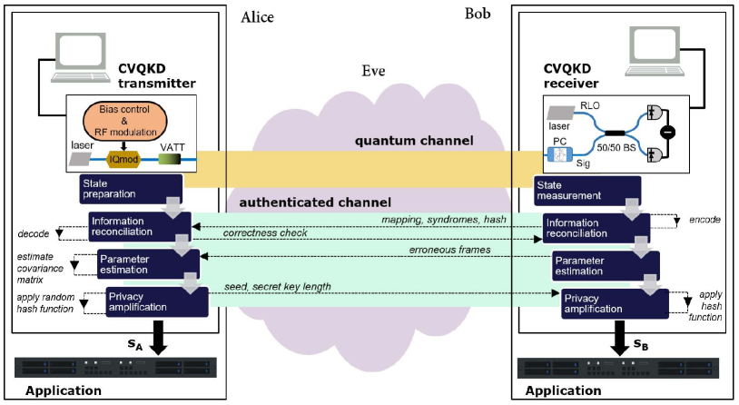
Figure 1: Composability in continuous-variable quantum key distribution (CVQKD). Alice and Bob obtain bitstreams $s_{A}$ and $s_{B}$, respectively, after going through the different steps of the QKD protocol that involve both the quantum and authenticated channels, assumed to be in full control of Eve. Various dashed lines (with arrows) indicate local operations and classical communication. An application using a CVQKD system (transmitter and receiver) to provide composable security must satisfy certain criteria associated with correctness, robustness, and secrecy of the protocol [3, 4]. For instance, the condition Pr$[s_{A}\neq s_{B}]\leq\epsilon_{\rm cor}$ denotes $\epsilon$-correctness, and describes the failure probability of Alice and Bob having non-identical keys at the conclusion of the protocol. Details of our CVQKD implementation (including full forms of the acronyms used in this graphic) are presented in III.1 and III.2, and the details of the protocol operation can be found in III.4.

Amongst the many physical considerations included in the security proof, one is that the number of quantum states available to Alice and Bob are not infinite. Such finite-size corrections adversely affect the key length but are essential for the security assurance.

Another related property of a cryptographic key is composability [5], which allows specifying the security requirements for combining different cryptographic applications in a unified and systematic way. In the context of practical QKD, composability is of utmost importance because the secret keys obtained from a QKD protocol are almost always used in other applications, e.g. data encryption [3]. A QKD implementation that outputs a key not proven to be composable is thus practically useless.

In one of the most well-known flavours of QKD, the quantum information is coded in continuous variables, such as the amplitude and phase quadratures, of the optical field [6, 7, 8, 2]. Typical continuous-variable (CV)QKD protocols have been Gaussian-modulated coherent state (GMCS) implementations [9, 10, 11, 12], and finite-size effects were also considered, though the proof [13] was non-composable. Composable security in CVQKD was first proven and experimentally demonstrated using two-mode squeezed states, however, since the employed entropic uncertainty relation is not tight, the achievable communication distance was rather limited [14, 15].

Composable security proofs for CVQKD systems using coherent states and dual quadrature detection, first proposed in 2015 [4], have been progressively improved [16, 17, 18]. These proofs promise keys at distances much longer than in Ref. [14] apart from the advantage of dealing with coherent states, which are much easier to generate than squeezed states. Nonetheless, an experimental demonstration of composability has remained elusive, due to a combination of the strict security bounds (because of a complex parameter estimation routine), the large number of required quantum state transmissions (to keep the finite-size terms sufficiently low), and the stringent requirements on the tolerable excess noise.

In this article, we demonstrate a practical GMCS-CVQKD system that is capable of generating composable keys secure against collective attacks. We achieve this by deriving a new method for establishing confidence intervals that is compatible with collective attacks, which allows us to work on smaller (and thus more practical) block sizes than originally required [4]. On the experimental front, we are able to keep the excess noise below the null key length threshold by performing a careful analysis (followed by eradication or avoidance) of the various spurious noise components, and by implementing a machine learning framework for phase compensation [19].

After taking finite-size effects as well as confidence intervals from various system calibrations into account, we achieve a positive composable key length with merely $N\lesssim 3.5\times 10^{8}$ coherent states (also referred to as ‘quantum symbols’). With $N=10^{9}$, we obtain $>53.4$ Mbits worth of composably secure key material in the worst case.

II Composably secure key

In the security analysis, we assume collective attacks and take into account the finite number of coherent states transmitted by Alice and measured by Bob. A digital signal processing (DSP) routine yields the digital quantum symbols $\bar{Y}$ discretized with $d$ bits per quadrature and this stream is divided into $M$ frames for information reconciliation (IR), after which we perform parameter estimation (PE) and privacy amplification (PA); as visualized in Fig. 1. We derive the secret key bound for reverse reconciliation, i.e., Alice correcting her data according to Bob’s quantum symbols.

The (composable) secret key length $s_{n}$ for $n$ coherent state transmissions is calculated using tools from Refs. [4, 18] as well as new results presented in the following. The key length is bounded per the leftover hash lemma in terms of the smooth min-entropy $H_{\min}$ of the alphabet of $\bar{Y}$, conditioned on the quantum state of the eavesdropper $E$ [20]. From this we subtract the information reconciliation leakage $\mathrm{leak_{IR}}(n,\epsilon_{\mathrm{IR}})$ and obtain,

$$s_{n}^{\epsilon_{h}+\epsilon_{s}+\epsilon_{\mathrm{IR}}}\geq H_{\min}^{\epsilon_{s}}(\bar{Y}|E)_{\rho^{n}}-\mathrm{leak_{IR}}(n,\epsilon_{\mathrm{IR}})+2\log_{2}{(\sqrt{2}\epsilon_{h})}\,.$$ (1)

The security parameter $\epsilon_{h}$ characterizes the hashing function, $\epsilon_{s}$ is the smoothing parameter entering the smooth conditional min-entropy, and $\epsilon_{\mathrm{IR}}$ describes the failure probability of the correctness test after IR.

The probability $p^{\prime}$ that IR succeeds in a frame is related to the frame error rate (FER) by $p^{\prime}=1-$FER. All frames in which IR failed are discarded from the raw key stream, and this step thereby projects the original tensor product state $\rho^{n}\equiv\rho^{\otimes n}$ into a non i.i.d. state $\tau^{n}$. To take this into account, one replaces the smooth min-entropy term in Eq. (1) with the expression [18]:

$$H_{\min}^{\epsilon_{s}}(\bar{Y}|E)_{\tau^{n^{\prime}}}\geq H_{\min}^{\frac{p^{\prime}}{3}\epsilon_{s}^{2}}(\bar{Y}|E)_{\rho^{\otimes n^{\prime}}}+\log_{2}{\left(p^{\prime}-\frac{p^{\prime}}{3}\epsilon_{s}^{2}\right)}\,,$$ (2)

where $n^{\prime}=np^{\prime}$ is the number of quantum symbols remaining after error correction.

The asymptotic equipartition property (AEP) bounds the conditional min-entropy by the von-Neumann conditional entropy,

$$H_{\min}^{\delta}(\bar{Y}|E)_{\rho^{\otimes n^{\prime}}}\geq n^{\prime}H(\bar{Y}|E)_{\rho}-\sqrt{n^{\prime}}\,\Delta_{\mathrm{AEP}}(\delta,d)\ ,$$

where

$$\Delta_{\mathrm{AEP}}(\delta,d)\leq 4(d+1)\sqrt{\log_{2}{(2/\delta^{2})}}\ ,$$ (3)

is an improved penalty in comparison to Ref. [4, 18], and is proven in the Supplement.

The conditional von-Neumann entropy is given by

$$H(\bar{Y}|E)_{\rho}=H(\bar{Y})_{\rho}-I(\bar{Y};E)_{\rho}\,.$$ (4)

We estimate the first term directly from the data (up to a probability not larger than $\epsilon_{\mathrm{ent}}$; further details regarding the confidence intervals are in the Supplement). The second term is bound by the Holevo information,

$$I(\bar{Y};E)_{\rho}\leq I(Y;E)_{\rho}\leq I(Y;E)_{\rho_{G}}\ ,$$

where $Y$ is the continuous version of $\bar{Y}$ and $I(Y;E)_{\rho_{G}}$ is the Holevo information obtained after using the extremality property of Gaussian attacks.

The Holevo information is estimated by evaluating the covariance matrix using worst-case estimates for its entries based on confidence intervals. We improved the confidence intervals of Ref. [4] by exploiting the properties of the beta distribution. Let $\hat{x}$, $\hat{y}$, $\hat{z}$ be the estimators for the variance of the transmitted ensemble of coherent states, the received variance and the co-variance, respectively. The true values $y$ and $z$ are bound by

$$y \leq\left(1+\delta_{\text{Var}}(n,\epsilon_{\text{PE}}/2)\right)\hat{y}\ ,$$ (5)

$$z \geq\left(1-2\delta_{\text{Cov}}(n,\epsilon_{\text{PE}}/2)\frac{\sqrt{\hat{x}\hat{y}}}{\hat{z}}\right)\hat{z}\ ,$$ (6)

with $\epsilon_{\text{PE}}$ denoting the failure probability of parameter estimation, and

$$\delta_{\mathrm{Var}}(n,\epsilon) =a^{\prime}\left(\epsilon/6\right)\left(1+\frac{120}{\epsilon}e^{-\frac{n}{16}}\right)-1\ ,$$

$$\delta_{\mathrm{Cov}}(n,\epsilon) =\frac{1}{2}\left[\frac{a^{\prime}\left(\epsilon/6\right)-b^{\prime}\left(\epsilon/6\right)}{2}+a^{\prime}\left(\frac{\epsilon^{2}}{324}\right)-b^{\prime}\left(\frac{\epsilon^{2}}{324}\right)\right]$$

being the new confidence intervals (derived in the Supplement). In the above equations,

$$a^{\prime}\left(\epsilon\right) =2\left[1-\mathrm{invcdf}_{\mathrm{Beta}(n/2,n/2)}\left(\epsilon\right)\right]\,,$$

$$b^{\prime}\left(\epsilon\right) =2\,\mathrm{invcdf}_{\mathrm{Beta}(n/2,n/2)}\left(\epsilon\right)\,.$$

As detailed in section IV, the (length of the) secret key we eventually obtain in our experiment requires an order of magnitude lower $N$ due to these confidence intervals.

Finally, we remark here on a technical limitation arising due to the digitization of Alice’s and Bob’s data. In practice, it is impossible to implement a true GMCS protocol because the Gaussian distribution is both unbounded and continuous, while the devices used in typical CVQKD systems have a finite range and bit resolution [21]. In our work, we consider a range of 7 standard deviations and use $d=6$ bits (leading to a constellation with $2^{2d}=4096$ coherent states), which per recent results [22, 23], should suffice to minimise the impact of digitization on the security of the protocol.

III Experiment

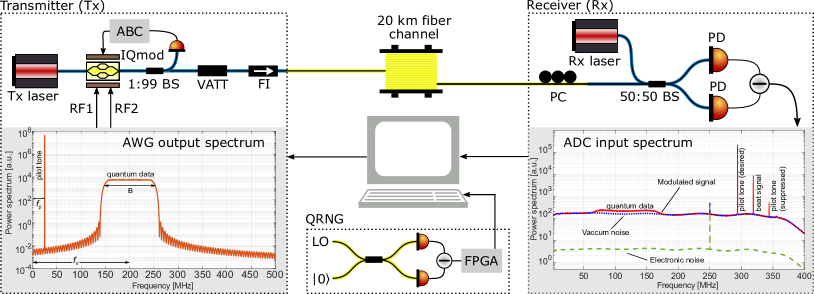
Figure 2: Schematic of the experiment. The transmitter (Tx) and receiver (Rx) were built from polarization maintaining fiber components. The transmitter comprised a 1550 nm continuous-wave laser (Tx laser), an in-phase and quadrature electro-optic modulator (IQmod) with automatic bias controller (ABC) for carrier suppression and single sideband modulation, and a variable attenuator (VATT) and faraday isolator (FI). An arbitrary waveform generator (AWG) with 16 bit resolution and sampling rate of 1 GSps supplied waveforms RF1 and RF2 for driving IQmod. A quantum random number generator (QRNG) delivered Gaussian-distributed symbols for discrete Gaussian modulation of coherent states. The receiver comprised a laser (Rx laser; same type as Tx laser), a polarization controller (PC) to tune the incoming signal field’s polarization, a symmetric beam splitter followed by a balanced detector for radio-frequency heterodyne detection. The detector’s output was sampled by a 16 bit analog-to-digital converter (ADC) at 1 GSps. BS: beam splitter, PD: photo detector. Left inset: Power spectrum of the complex waveform RF1 + $\iota$ RF2 driving the IQmod. Right inset: Power spectra of the receiver from 3 different measurements described in section III.2. The noise peak at 250 MHz is an interleaving spur of the ADC.

Figure 2 shows the schematic of our setup, with the caption detailing the components and their role briefly. Below we summarize the setup’s operation, calibration measurements, and our protocol implementation. In the Supplement, we describe the different functional blocks of Fig. 2 in further detail.

III.1 Transmitter (Tx)

We performed optical single sideband modulation with carrier suppression (OSSB-CS) using an off-the-shelf IQ modulator and automatic bias controller (ABC). An arbitrary waveform generator (AWG) was connected to the RF ports to modulate the sidebands. The coherent states were produced in a $B=100\,$MHz wide frequency sideband, shifted away from the optical carrier [24, 25]. The random numbers that formed the complex amplitudes of these coherent states were drawn from a Gaussian distribution, obtained by transforming the uniform distribution of a vacuum-fluctuation based quantum random number generator (QRNG), with a security parameter $\epsilon_{\text{qrng}}=2\times 10^{-6}$ [26].

To this wideband ‘quantum data’ signal, centered at $f_{u}=200\,$MHz, we multiplexed in frequency a ‘pilot tone’ at $f_{p}=25\,$MHz for sharing a phase reference with the receiver [27, 28, 29, 30]. The left inset of Fig. 2 shows the complex spectra of the RF modulation signal.

III.2 Receiver (Rx)

After propagating through the quantum channel—a 20 km long standard single mode fiber spool—the signal field’s polarization was manually tuned to match the polarization of the real local oscillator (RLO) for heterodyning [27, 28, 29]. The Rx laser that supplied the RLO was free-running with respect to the Tx laser and detuned in frequency by $\sim 320\,$ MHz, giving rise to a beat signal, as labelled in the solid-red spectral trace in the right inset of Fig. 2. The quantum data band and pilot tone generated by the AWG are also labelled. Due to finite OSSB [25], a suppressed pilot tone is also visible; the corresponding suppressed quantum band was however outside the receiver bandwidth (we used a low pass filter with a cutoff frequency around 360 MHz at the output of the heterodyne detector).

In separate measurements, we also measured the vacuum noise (Tx laser off, Rx laser on) and the electronic noise of the detector (both Tx and Rx lasers off), depicted by the dotted-blue and dashed-green traces, respectively, in the right inset of Fig. 2. The clearance of the vacuum noise over the electronic noise is $>15\,$dB over the entire quantum data band.

III.3 Noise analysis & Calibration

Table 1: Experimental parameters. PNU: photon number units. The security parameter $\epsilon_{\text{qrng}}$ is limited by the digitization error of the ADC used in the QRNG, but could be improved using longer measurement periods [26].

Transmitter
Rate of coherent states, $B$	100 MSymbols/s
Modulation strength (channel input), $\mu$	1.45 PNU
Receiver calibration
Trusted efficiency (incl. optical loss), $\tau$	0.69
Trusted electronic noise, $t$	25.71$\,\times 10^{-3}$ PNU
Channel parameter estimation
Untrusted efficiency, $\eta$	0.35
Untrusted excess noise, $u$	6.30$\,\times 10^{-3}$ PNU
Information reconciliation
Signal-to-noise ratio	0.32
Frame error rate, FER	0.36%
Reconciliation efficiency, $\beta$	91.6%
Leaked bits	$1.60\times 10^{9}$
Secret key calculation
Raw key length (symbols), $N_{\text{PA}}$	$9.84\times 10^{8}$
Security parameters	$\epsilon_{h}=\epsilon_{\text{cal}}=\epsilon_{s}=\epsilon_{\text{PE}}=10^{-10}$, $\epsilon_{\text{qrng}}=2\times 10^{-6}$, $\epsilon_{\text{IR}}=10^{-12}$
Final secret key length (bits)	53452436

A careful choice of the parameters defining the pilot tone and the quantum data band, and their locations with respect to the beat signal is crucial in minimizing the excess noise. A strong pilot tone enables more accurate phase reference but at the expense of higher leakage in the quantum band and an increased number of spurious tones. The latter may arise as a result of frequency mixing of the (desired) pilot tone with e.g., the beat signal or the suppressed pilot tone. As can be observed in the right inset of Fig. 2, we avoided spurious noise peaks resulting from sum- or difference-frequency generation of the various discrete components (in the solid-red trace) from landing inside the wide quantum data band.

As is well known in CVQKD implementations, Alice needs to optimize the modulation strength of the coherent state alphabet at the input of the quantum channel to maximize the secret key length. For this, we connected the transmitter and receiver directly, i.e., without the quantum channel, and performed heterodyne measurements to calibrate the mean photon number $\mu$ of the resulting thermal state from the ensemble of generated coherent states, as explained in section III.1. The modulation strength can be controlled in a fine-grained manner using the electronic gain of the AWG and the optical attenuation from the VATT. The DSP that aided in this calibration is explained in detail in the supplement.

Since we conducted our experiment in the non-paranoid scenario [1, 21], i.e., we trusted some parts of the overall loss and excess noise by assuming them to be beyond Eve’s control, some extra measurements and calibrations for the estimation of trusted parameters become necessary. More specifically, we decomposed the total transmittance and excess noise into respective trusted and untrusted components. In the Supplement, we present the details of how we evaluated the trusted transmittance $\tau$ and trusted noise $t$ for our setup.

Table 1 presents the values of $\mu$, $\tau$ and $t$ pertinent to the experimental measurement described in section III.4. Let us remark here that in our work, we express the noise and other variance-like quantities, e.g., the modulation strength, in photon number units (PNU) as opposed to the traditional shot noise units (SNU) because the former is independent of quadratures, and in case of $\mu$, facilitates a comparison with discrete-variable (DV) QKD systems. Finally, note that we recorded a total of $10^{10}$ ADC samples for each of the calibration measurements, and all the acquired data was stored on a hard drive for offline processing.

III.4 Protocol operation

We connected the transmitter and receiver using the 20 km channel, optimized the signal polarization, and then collected heterodyne data using the same Gaussian distributed random numbers as mentioned in section III.3. Offline DSP [19] was performed at the receiver workstation to obtain the symbols that formed the raw key. The preparation and measurement was performed with a total of $10^{9}$ complex symbols, modulated and acquired in 25 blocks, each block containing $4\times 10^{7}$ symbols. After discarding some symbols due to a synchronization delay, Alice and Bob had a total of $N_{\text{IR}}=9.88\times 10^{8}$ correlated symbols at the beginning of the classical phase of the protocol; see Fig. 1.

Below we provide details of the actual protocol we implemented, where we assumed that the classical channel connecting Alice and Bob was already authenticated.

1. IR was based on a multi-dimensional scheme [32] using multi-edge-type low-density-parity-check error correcting codes [33]. Table 1 lists some parameters related to the operating regime and the performance of these codes; more information is available in the Supplement. As shown in Fig. 1, Bob sent the mapping and the syndromes, together with the hashes computed using a randomly chosen Toeplitz function, to Alice, who performed correctness confirmation and communicated it to Bob.

2. During PE, Alice estimated the entropy of the corrected symbols, and together with the symbols from the erroneous frames, i.e., frames that could not be reconciled successfully (and were publicly announced by Bob), Alice evaluated the covariance matrix. This was followed by evaluating the channel parameters as well as performing the ‘parameter estimation test’ (refer Theorem 2 in Ref. [4]) and getting a bound on Eve’s Holevo information. Using the expression for the secret key length with the security parameters from Table 1, Alice then calculated the number of bits expected in the output secret key in the worst-case scenario. This length was communicated together with a seed to Bob.

3. For PA, the shared seed from the previous step was used to select a random Toeplitz hash function by Alice and Bob, who then employed the high-speed and large-scale PA scheme [34] to generate the final secret key.

IV Results & Discussion

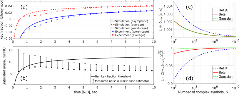
Figure 3: Composable SKF results. (a) Pseudo-temporal evolution of the composable SKF with the time parameter calculated as the ratio of the cumulative number $N$ of complex symbols available for the classical steps of the protocol and the rate $B$ at which these symbols are modulated. (b) Variation of untrusted noise $u$ measured in the experiment (lower point) and its worst-case estimator (upper point), and the noise threshold to beat in order to get a positive composable SKF. The reason for the deviation of the traces in (a) from the experimental data between 1 and 4 seconds is due to the slight increase in $u$. (c) and (d) Comparison of confidence intervals derived in this manuscript (Beta; solid-red trace and Gaussian; dashed-green trace) with those derived in the original composable security proof (Ref. [4]; dashed-blue trace) as a function of $N$.

Table 1 summarizes the relevant parameters in our experiment. Alice prepared an ensemble of $10^{9}$ coherent states, characterized by a modulation strength of 1.45 PNU, transmitted them over a 20 km channel to Bob, who measured them with a total excess noise $u+t=6.3+25.7=32.0\,$mPNU and a total transmittance $\eta\cdot\tau=0.35\cdot 0.69=0.24$ averaged over the amplitude and phase (I and Q) quadratures. With a total of $N_{\text{IR}}=9.88\times 10^{8}$ correlated symbols, Bob and Alice performed reverse reconciliation with an efficiency $\beta=$ 91.6% as explained in section III.4. Notably, due to the low frame error rate (FER = 0.0036) during IR, Alice and Bob were left with $N_{\text{PA}}=9.84\times 10^{8}$ symbols for performing the last classical step of the protocol.

Using the equations presented in section II, we can calculate the composably secure key length (in bits) for a certain number $N$ of the quantum symbols. We partitioned $N_{\text{IR}}$ in 25 blocks, estimated the key length considering the total number $N_{k}$ of symbols accumulated from the first $k$ blocks, for $k\in\{1,2,\ldots,25\}$. Dividing this length by $N_{k}$ yields the composable secret key fraction (SKF) in bits/symbols. If we neglect the time taken by data acquisition, DSP, and the classical steps of the protocol, i.e., only consider the time taken to modulate $N=N_{k}$ coherent states at the transmitter (at a rate $B=100\,$MSymbols/s), we can construct a hypothetical time axis to show the evolution of the CVQKD system.

Figure 3(a) depicts such a time evolution of the SKF after proper consideration to the finite-size corrections due to the average and worst-case (red and blue data points, respectively) values of the underlying parameters. Similarly, Fig. 3(b) shows the experimentally measured untrusted noise $u$ (lower squares) together with the worst-case estimator (upper dashes) calculated using $N_{k}$ in the security analysis. To obtain a positive key length, the worst-case estimator must be below the maximum tolerable noise—null key fraction threshold—shown by the solid line, and this occurs at $N/B\lesssim 3.5$ seconds.

Note that in reality, the DSP and classical data processing consume a significantly long time: In fact, we store the data from the state preparation and measurement stages on disks and perform these steps offline. The plots in Fig. 3 therefore may be understood to be depicting the time evolution of the SKF and the untrusted noise if the entire protocol operation was in real time.

Joining data from both I and Q quadratures bestowed $2N_{\text{PA}}=2\times 9.84\times 10^{8}$ real symbols, from which we then obtain a secret key with length $l=53452436$ bits, implying a worst-case SKF = $0.027\,$bits/symbol. Referring to Fig. 3(a), the solid-blue and dashed-red traces simulate the SKF in the worst-case and average scenarios, respectively, while the dotted-black trace shows the asymptotic SKF value obtainable with the given channel parameters; refer Table 1. Per projections based on the simulation, the worst-case composable SKF should be within 1% of the asymptotic value for $N\approx 10^{12}$ complex symbols.

From a theoretical perspective, the reason for being able to generate a positive composable key length with a relatively small number of coherent states ($N\lesssim 3.5\times 10^{8}$) can mainly be attributed to the improvement in confidence intervals during PE; refer equations 5 and 6. Figures 3(c) and (d) quantitatively compare the scaling factor in the RHS of these equations, respectively, as a function of $N$ for three different distributions. The estimators $\hat{x}$, $\hat{y}$, $\hat{z}$ for this purpose are the actual values obtained in our experiment and we used an $\epsilon_{\text{PE}}=10^{-10}$. The difference between the confidence intervals used in Ref. [4] (suitably modified here for a fair comparison) with those derived here, based on the Beta distribution, is quite evident at lower values of $N$, as visualized by comparing the dashed-blue trace with the solid-red one.

Since the untrusted noise has a quadratic dependence on the covariance in contrast to variance where the dependence is linear, a method that tightens the confidence intervals for the covariance can be expected to have a large impact on the final composable SKF. In fact, according to simulation, our implementation would have required almost an order of magnitude higher $N_{\text{PA}}$ ($\gtrsim 7.5\times 10^{9}$) using the confidence intervals of Ref. [4] to achieve the peak SKF depicted by the rightmost blue data point in Fig. 3(a).

The dashed-green trace shows the confidence intervals also based on the Beta distribution, and a further assumption of the underlying data, i.e., the I and Q quadrature symbols, following a Gaussian distribution (more details provided in the Supplement). This however may restrict the security analysis to Gaussian collective attacks, therefore, we do not make this assumption in our calculations. The advantage of this method would however be even tighter confidence intervals, and thus, even lower requirements on $N$ for obtaining a composable key with positive length.

On the practical front, a reasonably large transmission rate $B=100\,$MSymbols/s of the coherent states together with the careful analysis and removal of excess noise (refer section III.3 for more details) enables an overall fast, yet low-noise and highly stable system operation, critical in quickly distributing raw correlations of high quality and keeping the finite-size corrections minimal.

V Conclusion & Outlook

Due to its similarity to coherent telecommunication systems, continuous-variable quantum key distribution (CVQKD) based on coherent states is perhaps the most cost-effective solution for widespread deployment of quantum cryptography at access network scales ($10-50\,$km long quantum channels). However, CVQKD protocols have lagged behind their discrete-variable counterparts in terms of security, particularly, in demonstrating composability and robustness against finite-size effects. In this work, we have implemented a prepare-and-measure Gaussian-modulated coherent state CVQKD protocol that operates over a 20 km long quantum channel connecting Alice and Bob, who, at the end of the protocol obtain a composable secret key that takes finite-size effects into account and is protected against collective attacks. Our achievement was enabled by means of several novel advances in the theoretical security analysis and technical improvements on the experimental front. Furthermore, by using a real local oscillator at the receiver, we enhance the practicality as well as the security of the QKD system against hacking.

In conclusion, we believe this is a significant advance that demonstrates practicality, performance, and security of CVQKD implementations operating in the low-to-moderate channel loss regime. With an order of magnitude larger $N$ and half the current value of $u$, we expect to obtain a non-zero length of the composable key while tolerating channel losses around 8 dB, i.e., distances up to $\sim 40\,$km (assuming an attenuation factor of 0.2 dB/km). This should be easily achievable with some improvements in the hardware as well as the digital signal processing. We therefore expect that in the future, users across a point-to-point link could use the composable keys from our CVQKD implementation to enable real applications such as secure data encryption, thus ushering in a new era for CVQKD.

References

- [1] V. Scarani et al. The security of practical quantum key distribution. Reviews of Modern Physics, 81(3):1301–1350, 2009.
- [2] S. Pirandola et al. Advances in quantum cryptography. Advances in Optics and Photonics, 12(4):1012, dec 2020.
- [3] J. Müller-Quade and R. Renner. Composability in quantum cryptography. New Journal of Physics, 11, 2009.
- [4] A. Leverrier. Composable security proof for continuous-variable quantum key distribution with coherent states. Physical Review Letters, 114(7), 2015.
- [5] R. Canetti. Universally composable security: a new paradigm for cryptographic protocols. In Proceedings 42nd IEEE Symposium on Foundations of Computer Science, pp. 136–145, 2001.
- [6] T. C. Ralph. Continuous variable quantum cryptography. Phys. Rev. A, 61:010303, Dec 1999.
- [7] E. Diamanti and A. Leverrier. Distributing secret keys with quantum continuous variables: Principle, security and implementations. Entropy, 17(9):6072–6092, 2015.
- [8] F. Laudenbach et al. Continuous-Variable Quantum Key Distribution with Gaussian Modulation-The Theory of Practical Implementations. Advanced Quantum Technologies, 1(1):1800011, aug 2018.
- [9] P. Jouguet et al. Experimental demonstration of long-distance continuous-variable quantum key distribution. Nature Photonics, 7(5):378–381, 2013.
- [10] D. Huang et al. Long-distance continuous-variable quantum key distribution by controlling excess noise. Scientific Reports, 6(1):19201, may 2016.
- [11] T. Wang et al. High key rate continuous-variable quantum key distribution with a real local oscillator. Optics Express, 26(3):2794, feb 2018.
- [12] H. Wang et al. High-speed Gaussian-modulated continuous-variable quantum key distribution with a local local oscillator based on pilot-tone-assisted phase compensation. Optics Express, 28(22):32882, oct 2020.
- [13] A. Leverrier et al. Finite-size analysis of a continuous-variable quantum key distribution. Physical Review A, 81(6):1–11, 2010.
- [14] F. Furrer et al. Continuous variable quantum key distribution: Finite-key analysis of composable security against coherent attacks. Phys. Rev. Lett., 109:100502, Sep 2012.
- [15] T. Gehring et al. Implementation of continuous-variable quantum key distribution with composable and one-sided-device-independent security against coherent attacks. Nature Communications, 6:1–7, 2015.
- [16] C. Lupo et al. Continuous-variable measurement-device-independent quantum key distribution: Composable security against coherent attacks. Phys. Rev. A, 97:052327, May 2018.
- [17] P. Papanastasiou and S. Pirandola. Continuous-variable quantum cryptography with discrete alphabets: Composable security under collective Gaussian attacks. Physical Review Research, 3(1):013047, jan 2021.
- [18] S. Pirandola. Limits and security of free-space quantum communications. Physical Review Research, 3(1):013279, mar 2021.
- [19] H.-M. Chin et al. Machine learning aided carrier recovery in continuous-variable quantum key distribution. npj Quantum Information, 7(1):20, dec 2021.
- [20] M. Tomamichel. A Framework for Non-Asymptotic Quantum Information Theory. PhD thesis, ETH Zurich, mar 2012.
- [21] P. Jouguet et al. Analysis of imperfections in practical continuous-variable quantum key distribution. Physical Review A, 86(3):1–9, 2012.
- [22] C. Lupo. Towards practical security of continuous-variable quantum key distribution. Physical Review A, 102(2):1–10, 2020.
- [23] A. Denys et al. Explicit asymptotic secret key rate of continuous-variable quantum key distribution with an arbitrary modulation. Quantum, 5:540, September 2021.
- [24] A. M. Lance et al. No-Switching Quantum Key Distribution Using Broadband Modulated Coherent Light. Physical Review Letters, 95(18):180503, 2005.
- [25] N. Jain et al. Modulation leakage vulnerability in continuous-variable quantum key distribution. Quantum Science and Technology, 6(4), 2021.
- [26] T. Gehring et al. Homodyne-based quantum random number generator at 2.9 Gbps secure against quantum side-information. Nature Communications, 12(1):1–11, 2021.
- [27] B. Qi et al. Generating the local oscillator “locally” in continuous-variable quantum key distribution based on coherent detection. Physical Review X, 5(4):1–12, 2015.
- [28] D. B. S. Soh et al. Self-referenced continuous-variable quantum key distribution protocol. Physical Review X, 5(4):1–15, 2015.
- [29] D. Huang et al. High-speed continuous-variable quantum key distribution without sending a local oscillator. Optics letters, 40(16):3695–8, 2015.
- [30] S. Kleis et al. Continuous variable quantum key distribution with a real local oscillator using simultaneous pilot signals. Optics Letters, 42(8):1588–1591, 2017.
- [31] Assuming symmetry between the quadratures, the modulation variance in SNU.
- [32] A. Leverrier et al. Multidimensional reconciliation for a continuous-variable quantum key distribution. Phys. Rev. A, 77:042325, Apr 2008.
- [33] H. Mani et al. Multiedge-type low-density parity-check codes for continuous-variable quantum key distribution. Phys. Rev. A, 103:062419, Jun 2021.
- [34] B.-Y. Tang et al. High-speed and Large-scale Privacy Amplification Scheme for Quantum Key Distribution. Scientific Reports, pp. 1–8, 2019.