Obtaining efficient thermal engines from interacting Brownian particles under time dependent periodic drivings

Abstract

We introduce an alternative route for obtaining reliable cyclic engines, based on interacting Brownian particles under time-periodic drivings. General expressions for the thermodynamic fluxes, such as power and heat, are obtained using the framework of Stochastic Thermodynamics. Several protocols for optimizing the engine performance are considered, by looking at system parameters such as the output forces and their phase-difference. We study both work-to-work and heat-to-work engines. Our results suggest that carefully designed interactions between particles can lead to more efficient engines.

I Introduction

Small scale engines operating out of equilibrium have received a substantial increase of attention in the last years, especially because several process in nature (mechanical, biological, chemical and others) are related to some kind of energy conversion (e.g. mechanical into chemical and vice-versa) Seifert (2012); Liepelt and Lipowsky (2007, 2009). The constant fluctuating flow of energy constitutes a fundamental feature fueling the operation of nonequilibrium engines which is well described by the framework of Stochastic Thermodynamics Seifert (2012).

Entropy production plays a fundamental role in Nonequilibrium Thermodynamics. It satisfies fluctuation theorems Crooks (1999); Jarzynski (1997) and bounds such as the Thermodynamic Uncertainty Relations (TURs) Barato and Seifert (2015); Pietzonka et al. (2016); Barato et al. (2018, 2019); Proesmans and Van den Broeck (2017a); Harunari et al. (2020); Hasegawa and Van Vu (2019); Van Vu and Hasegawa (2020) and can be extended for deriving general bounds between power, efficiency and dissipation Pietzonka and Seifert (2018). Here we look at a case-study of a cyclic heat engines in which the nonequilibrium features are due to distinct thermal reservoirs and time-dependent external forces.

Brownian particles are often at the core of nano-scaled heat engines Martínez et al. (2016); Krishnamurthy et al. (2016); Blickle and Bechinger (2012); Proesmans et al. (2016a); Quinto-Su (2014); Jones et al. (2015); Albay et al. (2018); Kumar and Bechhoefer (2018); Paneru and Kyu Pak (2020); Li et al. (2019). Most of them are based on single particle engines and have been studied for theoretical Noa et al. (2020); Proesmans et al. (2015); Rana et al. (2014); Schmiedl and Seifert (2007); Hoppenau et al. (2013); Tu (2014); Chvosta et al. (2010); Verley et al. (2014); Imparato et al. (2007); Plata et al. (2020) and experimental Martínez et al. (2016); Albay et al. (2021); Jun et al. (2014) settings. On the other hand, the number of studies on the thermodynamic properties of interacting chains of particles are limited and often constrained to time-independent driving Park et al. (2016); Akasaki et al. (2020); Li et al. (2019). The scarcity of results, together the richness of such system, raises distinct and relevant questions about the interaction contribution to the performance, the interplay between interaction and driving forces and choice of protocol optimization. The latter is a field in itself with a lot of recent works focusing on the optimization of distinct engines in terms of efficiency and/or power Curzon and Ahlborn (1975); Schmiedl and Seifert (2007); Holubec (2014); Harunari et al. (2021); Golubeva and Imparato (2012).

In this work we conciliate above issues by introducing an interacting version of the underdamped Brownian Duet Proesmans and Van den Broeck (2017b), in which each particle is subject to a distinct thermal bath and driving force. The existence of distinct parameters (interaction between particles, strength of forces, phase difference and frequency) provides several routes for tackling optimization that will be analyzed using the framework of stochastic thermodynamics. The introduction of interaction will provide additional control and also enhancement of power and/or efficiency. Distinct types of optimization will be introduced and analyzed: maximization of output power and efficiency with respect to the output forces, phase difference between external forces and interaction.

Two different situations will be addressed. Initially, we consider the case in which the thermal baths have the same temperature (interacting particle work-to-work converter) Proesmans et al. (2016a). We then advance beyond the work-to-work converter by including a temperature difference between thermal baths and general predictions are obtained for distinct set of temperatures.

The paper is structured as follows: in Section II we introduce the model and the main expressions for relevant quantities. In Section III, we analyze the engine performance for distinct regime operations. Conclusions are drawn in Section IV.

II Thermodynamics of interacting Brownian engines

The model is composed by two interacting underdamped Brownian particles with equal mass $m$, each one subject to a distinct external force and placed in contact with a thermal bath of temperature $T_{i}$, $i=\{1,2\}$. Their positions and velocities, $x_{i}$ and $v_{i}$, evolve in time according to the following set of Langevin equations:

$$\derivative{v_{1}}{t}=\frac{1}{m}F_{1}^{*}(x_{1},x_{2})+\frac{1}{m}F_{1}(t)-\gamma v_{1}+\zeta_{1},$$ (1)

$$\derivative{v_{2}}{t}=\frac{1}{m}F_{2}^{*}(x_{1},x_{2})+\frac{1}{m}F_{2}(t)-\gamma v_{2}+\zeta_{2},$$ (2)

and

$$\derivative{x_{1}}{t}=v_{1},\quad\derivative{x_{2}}{t}=v_{2},$$ (3)

respectively. There are eight forces acting on the system: two forces $F_{i}^{*}(x_{1},x_{2})$, related to the harmonic potentials and the interaction between particles, two external driving components $F_{i}(t)$, friction forces $-\gamma v_{i}$ (with $\gamma$ denoting the friction parameter) and stochastic forces $\zeta_{i}(t)$. The former can be written as the derivative of a potential $V_{i}$ given by $F_{i}^{*}(x_{1},x_{2})=-\partial V_{i}/\partial x_{i}$, whereas the stochastic forces are described as a white noise: $\expectationvalue{\zeta_{i}(t)}=0$ and $\expectationvalue{\zeta_{i}(t)\zeta_{j}(t^{\prime})}=2\gamma k_{\text{B}}T_{i}\delta_{ij}\delta(t-t^{\prime})/m$. The above set of Langevin equations are associated with the probability distribution $P(x_{1},x_{2},v_{1},v_{2},t)$ having its time evolution governed by Fokker-Planck-Kramers (FPK) equation:

$$\frac{\partial P}{\partial t}=-\sum_{i=1}^{2}\left(v_{i}\frac{\partial P}{\partial x_{i}}+[F_{i}^{*}+F_{i}(t)]\frac{\partial P}{\partial v_{i}}+\frac{\partial J_{i}}{\partial v_{i}}\right),$$ (4)

where

$$J_{i}=-\gamma v_{i}P-\frac{\gamma k_{\mbox{\tiny B}}T_{i}}{m}\frac{\partial P}{\partial v_{i}}.$$ (5)

If the temperatures of both particles are equal and the external forces are absent, the probability distribution approaches for large times the Gibbs equilibrium distribution, $P^{\text{eq}}(x_{1},x_{2},v_{1},v_{2})\propto e^{-E/k_{\mbox{\tiny B}}T}$, where $E=\sum_{i}(mv_{i}^{2}/2+V_{i})$ is the total energy of the system. From now on, we shall consider harmonic potentials $V_{i}=k_{i}x_{i}^{2}/2+\kappa(x_{i}-x_{j})^{2}/2$, whose associate forces read $F_{i}^{*}=-kx_{i}-\kappa(x_{i}-x_{j})$. The time evolution of a generic average $\expectationvalue{x_{i}^{n}v_{j}^{m}}$ can be obtained from the FPK equation, Eq. (4), and performing appropriate partial integrations by assuming that $P(x_{1},x_{2},v_{1},v_{2},t)$ and its derivatives vanish when $x_{i}$ or $v_{i}$ approaches to $\pm\infty$. More specifically, we are interested in obtaining expressions for thermodynamic quantities, such as the heat exchanged between particle $i$ and the reservoir and the work rate performed by each external force over its particle. Their expressions can be obtained from the time evolution of mean energy $\langle E\rangle$ together the FPK equation and assumes a form consistent with the first law of Thermodynamics Tomé and de Oliveira (2010); Seifert (2012); Van den Broeck and Esposito (2010):

$$\frac{d\langle E\rangle}{dt}=-\sum_{i=1}^{2}(\dot{W}_{i}+\dot{Q}_{i}),$$ (6)

where $\dot{W}_{i}$ is work done over particle $i$, due to the external force $F_{i}(t)$,

$$\dot{W}_{i}=-mF_{i}(t)\expectationvalue{v_{i}},$$ (7)

and $\dot{Q}_{i}$ is the heat delivered to reservoir $i$. An expression for the heat can be derived from the above two equations:

$$\dot{Q}_{i}=\gamma\left(m\expectationvalue{v_{i}^{2}}-k_{\text{B}}T_{i}\right).$$ (8)

Similarly, the time evolution of system entropy $S=-k_{\mbox{\tiny B}}\langle\ln P(x_{1},x_{2},v_{1},v_{2})\rangle$ is the difference between entropy production rate $\sigma$ and entropy flux rate $\Phi$ to/from the system to/from the thermal reservoir given by Tomé and de Oliveira (2010); Seifert (2012); Van den Broeck and Esposito (2010)

$$\sigma=\frac{m}{\gamma}\sum_{i=1}^{2}\frac{1}{T_{i}}\int\frac{J_{i}^{2}}{P}dx_{1}dx_{2}dv_{1}dv_{2},$$ (9)

and

$$\Phi=-\sum_{i=1}^{2}\frac{m}{T_{i}}\int v_{i}J_{i}dx_{1}dx_{2}dv_{1}dv_{2},$$ (10)

respectively. Note that $\sigma\geq 0$ (as expected), whereas $\Phi$ can be conveniently rewritten in terms of the ratio between $\dot{Q}_{i}$ and the temperature $T_{i}$:

$$\Phi=\sum_{i}\gamma\left(\frac{m\langle v_{i}^{2}\rangle}{T_{i}}-k_{\text{B}}\right)=\sum_{i=1}^{2}\frac{\dot{Q}_{i}}{T_{i}}.$$ (11)

It is convenient to relate averages $\langle v_{i}\rangle$’s and $\langle v_{i}^{2}\rangle$’s by means their covariances $b_{ij}^{vv}(t)\equiv\langle v_{i}v_{j}\rangle(t)-\langle v_{i}\rangle(t)\langle v_{j}\rangle(t)$. For simplifying matters, from now on we set $m=k_{B}=1$. Due to the interaction between particles, $b_{ij}^{vv}(t)$ also depends on covariances $b_{ij}^{xx}(t)$’s and $b_{ij}^{xv}(t)$’s ($x$ and $v$ attempting to the position and velocity of the $i$-th and $j-$th particles, respectively). Their time evolutions are straightforwardly obtained from Eq. (4), whose expression for $b_{11}^{vv}$ is given by

$$b_{11}^{vv}=\frac{T_{1}+T_{2}}{2}+\frac{\left(T_{1}-T_{2}\right)}{2}\frac{\gamma^{2}(\kappa+k)}{\left[\kappa^{2}+\gamma^{2}(\kappa+k)\right]},$$ (12)

and $b_{22}^{vv}$ is obtained just by exchanging $1\leftrightarrow 2$.

II.1 Periodically driving forces

Having obtained the general expressions for a chain of two interacting particles, we are now in position to get expressions in the presence of external forces. Our aim is to study the effect that interactions have on the performance of an engine. To do this, we will focus on the simplest case in which particles are subject to harmonic time-dependent forces $F_{i}(t)$ of different amplitude, same frequency $\omega$, but with a lag $\delta$ between them Proesmans et al. (2016a); Proesmans and Van den Broeck (2017b); Fiore and de Oliveira (2019); Akasaki et al. (2020)

$$F_{1}(t)=X_{1}\cos{(\omega t)},$$ (13)

and

$$F_{2}(t,\delta)=X_{2}\cos{[\omega(t-\delta)]},$$ (14)

respectively. The system will relax to a time-periodic steady state with $\overline{\dot{Q}}_{1}+\overline{\dot{Q}}_{2}=-(\overline{\dot{W}}_{1}+\overline{\dot{W}}_{2})$, where each mean work $\overline{\dot{W}}_{i}$ and heat ${\overline{\dot{Q}}_{i}}$ are given by

$$\overline{\dot{W}}_{i}=-\frac{\omega}{2\pi}\int_{0}^{2\pi/\omega}F_{i}(t)\langle v_{i}\rangle(t)dt,$$ (15)

and

$${\overline{\dot{Q}}_{i}} = \frac{\omega\gamma}{2\pi}\int_{0}^{2\pi/\omega}\langle v_{i}\rangle^{2}dt-\overline{\kappa}(T_{i}-T_{j}),$$ (16)

respectively, where $\overline{\kappa}$ is the thermal conduction given by $\overline{\kappa}=\gamma\kappa^{2}/[2\kappa^{2}+2\gamma^{2}(\kappa+k)]$ Morgado and Soares-Pinto (2009); Tomé and de Oliveira (2010). The steady entropy production over a cycle is promptly obtained from Eq. (11) and it is related with average work and heat according to the expression:

$$\overline{\sigma}=\frac{4T^{2}}{4T^{2}-\Delta T^{2}}\left[-\frac{1}{T}(\overline{\dot{W}}_{1}+\overline{\dot{W}}_{2})+(\overline{\dot{Q}}_{1}-\overline{\dot{Q}}_{2})\frac{\Delta T}{2T^{2}}\right],$$ (17)

where $T=(T_{1}+T_{2})/2$ and $\Delta T=T_{2}-T_{1}$. It can also be viewed as sum of two components: ${\overline{\sigma}}=\Phi_{T}+{\overline{\Phi}_{f}}$, where the former, $\Phi_{T}$, due to the difference of temperatures is given by

$$\Phi_{T}=\frac{4\overline{\kappa}\Delta T^{2}}{4T^{2}-\Delta T^{2}},$$ (18)

and the latter, due to the external forces, is given by

$${\overline{\Phi}_{f}}={\tilde{L}}_{11}X_{1}^{2}+({\tilde{L}}_{12}+{\tilde{L}}_{21})X_{1}X_{2}+{\tilde{L}}_{22}X_{2}^{2},$$ (19)

respectively. Above expressions are exact and hold beyond linear regime (large forces and/or large difference of temperatures) between thermal baths. In order to relate them with thermodynamic fluxes and forces, we are going to perform the analysis of a small temperature difference $\Delta T$ between thermal baths. In such case, we introduce the forces $f_{1}=X_{1}/T$, $f_{2}=X_{2}/T$ and $f_{T}=\Delta T/T^{2}$, in such a way that

$$\overline{\sigma}\approx J_{1}f_{1}+J_{2}f_{2}+J_{T}f_{T},$$ (20)

where flux $i$ ($i=1,2$ or $T$) is associate with force $f_{i}$ and given by the following expressions $\overline{\dot{W}}_{1}=-TJ_{1}f_{1}$, $\overline{\dot{W}}_{2}=-TJ_{2}f_{2}$ and $\overline{\dot{Q}}_{1}-\overline{\dot{Q}}_{2}=2J_{T}f_{T}$. From them, one can obtain Onsager coefficients $J_{1}=L_{11}f_{1}+L_{12}f_{2}$, $J_{2}=L_{21}f_{1}+L_{22}f_{2}$ and $J_{T}=L_{TT}f_{T}$, whose main expressions are listed below

$$L_{11}=L_{22}=\left(\frac{T\gamma\omega^{2}}{2}\right)\frac{\gamma^{2}\omega^{2}+\left(\omega^{2}-(k+\kappa)\right)^{2}+\kappa^{2}}{\left[\gamma^{2}\omega^{2}+\left(\omega^{2}-k\right)^{2}\right]\left[\gamma^{2}\omega^{2}+(\omega^{2}-(k+2\kappa))^{2}\right]},$$ (21)

$$L_{12}=\left(\frac{T\kappa\omega}{2}\right)\frac{2\gamma\omega\left(\kappa+k-\omega^{2}\right)\cos(\delta\omega)-\left[\gamma^{2}\omega^{2}-(\omega^{2}-(k+\kappa))^{2}+\kappa^{2}\right]\sin(\delta\omega)}{\left[\gamma^{2}\omega^{2}+\left(\omega^{2}-k\right)^{2}\right]\left[\gamma^{2}\omega^{2}+(\omega^{2}-(k+2\kappa))^{2}\right]},$$ (22)

$$L_{21}=\left(\frac{T\kappa\omega}{2}\right)\frac{2\gamma\omega\left(\kappa+k-\omega^{2}\right)\cos(\delta\omega)+\left[\gamma^{2}\omega^{2}-(\omega^{2}-(k+\kappa))^{2}+\kappa^{2}\right]\sin(\delta\omega)}{\left[\gamma^{2}\omega^{2}+\left(\omega^{2}-k\right)^{2}\right]\left[\gamma^{2}\omega^{2}+(\omega^{2}-(k+2\kappa))^{2}\right]},$$ (23)

and

$$L_{TT}={\overline{\kappa}}T^{2},$$ (24)

respectively. All other Onsager coefficients are zero. We pause to make some comments: First, for $\Delta T=0$, expressions for $L_{ij}$’s ($i=1$ and 2) are exact and valid for arbitrary large values of $f_{i}$’s. Second, one can verify that $L_{11}=L_{22}\geq 0$ and $(L_{12}+L_{21})^{2}\leq 4L_{11}L_{22}$ in agreement with the second law of thermodynamics. Above conditions are promptly verified for all $k,\kappa$ and $\omega$. The non-diagonal Onsager coefficients $L_{12}$ and $L_{21}$ are not the same, except for the lagless case $\delta=0$. Third, in the regime of low and large frequencies, all coefficients behave as $\omega^{2}$ and $1/\omega^{2}$ (diagonal) and $1/\omega^{4}$ (non-diagonal for $\delta=0$), respectively. Fourth, the non-diagonal coefficients vanish for sufficiently weak interactions while the diagonal is finite, consistent with a quasi-decoupling between particles. Conversely, when the coupling parameter is very strong, $\kappa\to\infty$, all coefficients remain finite and coincide with those for one Brownian particle in a harmonic potential subjected to both external forces. Fifth, for large $\Delta T$, Eq. (16) states that the heat exchanged with the thermal bath $i$ has two contributions: the first, coming from external forces, has the form $A_{i}f_{i}^{2}+B_{i}f_{i}f_{j}+C_{i}f_{j}^{2}$ (with coefficients $A_{i},B_{i}$ and $C_{i}$ listed in Appendix .2) and it is strictly non-negative. Hence, coefficients satisfy $A_{i}\geq 0$ and $C_{i}\geq 0$ and $B_{i}^{2}-4A_{i}C_{i}\leq 0$. The second term, coming from the difference of temperatures, can be positive or negative depending on the sign of $T_{j}-T_{i}$. In the absence of external forces, the entropy production reduces to Eq. (18). Sixth, expressions for coefficients ${\tilde{L}}_{ij}$’s appearing in Eq. (19) (see Appendix .2) are exact and hold beyond linear regime listed (large forces and/or large difference of temperatures) between thermal baths.in Appendix .2. Seventh and last, the interplay between both terms can change the direction of the heat flowing per cycle, implying that the coupling parameter can change the regime of operation of the engine, from heater to heat engine and vice-versa, as $\kappa$ is increased and decreased. Similar findings have also been observed for two coupled double-quantum-dots de Oliveira et al. (2021) and coupled spins Huang et al. (2014).

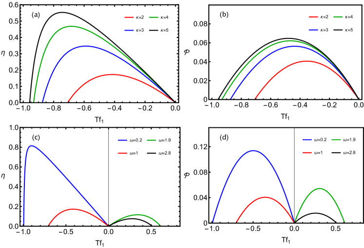
Figure 1: Panels $(a)$ and $(b)$ panels depict the efficiency $\eta$ and power output ${\cal P}$ versus $Tf_{1}$ for distinct $\kappa$’s and $\omega=1$. In $(b)$ and $(d)$, the same but for distinct $\omega$’s and $\kappa=2$. In all cases, we set $Tf_{2}=1,T=0.3,\delta=0$ and $k=0.1$.

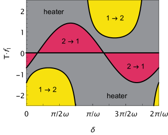
Figure 2: Phase diagram $Tf_{1}$ versus $\delta$ for the work-to-work converter. $1\rightarrow 2$/ $2\rightarrow 1$ and heater correspond to the (engine) regime in which there is the conversion from $\overline{\dot{W}}_{1}<0$ into $\overline{\dot{W}}_{2}>0$/vice-versa and $\overline{\dot{W}}_{1}>0$ and $\overline{\dot{W}}_{2}>0$, respectively. Parameters: $Tf_{2}=\gamma=\omega=1$, $k=0.1$, $T=0.3$ and $\kappa=2$.

Figure 3: For the same parameters from Fig. 1, the efficiency $\eta$ (left) and power output ${\cal{P}}$ (right) versus $Tf_{1}$ for distinct phase differences $\delta$’s. Dashed and continuous lines in left panel correspond to the conversion from $\overline{\dot{W}}_{1}$ into $\overline{\dot{W}}_{2}$ and vice-versa, respectively. Circles, stars and squares denote the maximum efficiency, maximum power and $Tf_{m}$, respectively.

III Efficiency

A generic system operates as an engine when parameters are set in such a way that a given amount of energy received is partially converted into power output ${\cal P}\geq 0$. A measure for the efficiency $\eta$ is given by the ratio between above quantities and constitutes a fundamental quantity for characterizing such conversion. Our aim here consists of exploring the role of distinct parameters, mainly the interaction between particles, in such a way that such system can operate as an efficient engine. By considering for instance the particle $i=2$ as the worksource, the engine regime implies that ${\cal P}={\overline{\dot{W}_{\rm 1}}}\geq 0$ and according to Eq. (16) the system will receive heat when $T_{1}>>T_{2}$ ($T_{2}>>T_{1}$), consistent with ${\overline{\dot{Q}_{\rm 1}}}<0$ (${\overline{\dot{Q}_{\rm 2}}}<0$). Conversely, when the difference of temperatures between thermal baths is small and/or when forces $f_{1}/f_{2}$ are large, both particles do not necessarily receive heat from the thermal bath and only input work (actually input power) can be converted into output work. Such class of engines, also known as work-to-work converter, will be analyzed next.

We shall split the analysis in the regime of equal and different temperatures. For both cases, we will investigate the machine performance with respect to the loading force $f_{1}$ and other parameters, such as interaction $\kappa$ and phase difference $\delta$.

III.1 work-to-work converter

Since for equal temperatures $\overline{\dot{Q}}_{1}$ and $\overline{\dot{Q}}_{2}$ are non negative, consistent with the system solely delivering heat to the thermal baths, Eq. (45) reduces to the ratio between worksources:

$$\eta\equiv-\frac{{\cal P}}{\overline{\dot{W}}_{\text{2}}}=-\frac{L_{11}f_{1}^{2}+L_{12}f_{1}f_{2}}{L_{21}f_{2}f_{1}+L_{22}f_{2}^{2}},$$ (25)

where the second right side of Eq. (25) was re-expressed in terms of Onsager coefficients and thermodynamic forces.

Fig. 1 depicts, for $\delta=0$, the main features of the efficiency and power output by analyzing the influence of interaction $\kappa$ and frequency $\omega$. We find that the interaction between particles improves substantially the machine performance. Properly tuning $\kappa$ not only changes the operation regime, from heater to a work-to-work converter (engine), but also increases the power, efficiency and the range of operation [e.g. the possible values of $f_{1}$ within the same engine regime, cf. panels (a) and (b)]. Unlike the engine, in the heater operation mode (often called dud engine), work is extracted from both worksources ($\overline{\dot{W}}_{1}$ and $\overline{\dot{W}}_{2}>0$). Contrariwise, the increase of frequency (lowering the driving period) reduces the machine efficiency. This can be understood by the fact that the system presents some inertia and does not properly respond to abrupt changes when frequency is large. The output force $f_{1}$ has opposite direction to $f_{2}$ when $k+\kappa>\omega^{2}$ and vice-versa, as depicted in panels (c) and (d).

Next, we examine the influence of a phase difference between harmonic forces, as depicted in Figs 2-4. The existence of a lag between driving forces not only controls the power and efficiency, but can also guide the operation modes of the system. In other words, depending on the value of $\delta$, the work is extracted from the worksource 1 and dumped into the worksource 2 ($\eta=-\overline{\dot{W}}_{2}/\overline{\dot{W}}_{1}$) or vice-versa ($\eta=-\overline{\dot{W}}_{1}/\overline{\dot{W}}_{2}$), both conversions are possible for the same output force or even none of them.

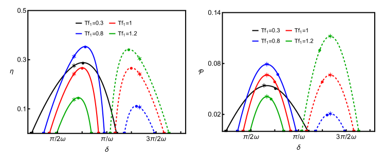
Figure 4: For the same parameters from Fig. 2, the efficiency $\eta$ (left) and power output ${\cal P}$ (right) versus phase difference $\delta$ for distinct $Tf_{1}^{\prime}s$. Continuous and dashed lines correspond to the conversion from $\overline{\dot{W}}_{2}$ into $\overline{\dot{W}}_{1}$ and vice-versa, respectively. Squares, stars and circles denote the $\delta_{m1}/\delta_{m2}$, maximum power and maximum efficiency, respectively.

Such changes of conversion in the operation model (see e.g. Fig. 2) share some similarities with some theoretical models for kinesin in which the range chemical potentials and mechanical forces can rule the energy conversion (chemical into mechanical and vice-versa) Liepelt and Lipowsky (2009).

Once introduced the main features about the model parameters and how they influence the machine performance, we are going to present distinct protocols for optimizing them.

III.1.1 Maximization with respect to the output force

The first (and simplest) maximization is carried out with respect to the output force $f_{1}$ and the other parameters are held fixed. Such optimizations have been performed in Refs. Proesmans et al. (2016b); Noa et al. (2020). Since ${\cal P}=\overline{\dot{W}}_{\text{1}}\geq 0$ the engine regime is delimited by the interval $0\leq\absolutevalue{f_{1}}\leq\absolutevalue{f_{m}}$ where $f_{m}\equiv-L_{12}f_{2}/L_{11}$. By adjusting the output forces $f_{1mP}$ and $f_{1mE}$ ensuring maximum power ${\cal P}_{mP}$ (with efficiency ${\eta}_{mP}$) and maximum efficiency ${\eta}_{mE}$ (with power ${\cal P}_{mE}$), we obtain the following expressions, expressed in terms of Onsager coefficients Proesmans et al. (2016b):

$$f_{1mE}=\frac{L_{22}}{L_{12}}\left(-1+\sqrt{1-\frac{L_{21}L_{12}}{L_{22}L_{11}}}\right)f_{2},$$ (26)

and

$$f_{1mP}=-\frac{1}{2}\frac{L_{12}}{L_{11}}f_{2},$$ (27)

respectively, with corresponding efficiencies

$$\eta_{mE,f_{1}}=-\frac{L_{12}}{L_{21}}+\frac{2L_{11}^{2}}{L_{21}^{2}}\left(1-\sqrt{1-\frac{L_{21}L_{12}}{L_{11}^{2}}}\right),$$ (28)

and

$$\eta_{mP,f_{1}}=\frac{L_{12}^{2}}{4L_{11}^{2}-2L_{21}L_{12}},$$ (29)

respectively, where the property $L_{22}=L_{11}$ has been used. Similar expressions are obtained for ${\cal P}_{mE}$ and ${\cal P}_{mP}$ by inserting $f_{1mE}$ and $f_{1mP}$ into the relation for ${\cal P}$. Maximum efficiencies are not independent from each other, but related via simple relation

$$\eta_{mP,f_{1}}=\frac{P_{mP,f_{1}}}{2P_{mP,f_{1}}-P_{mE,f_{1}}}\eta_{mE,f_{1}}.$$ (30)

respectively Proesmans et al. (2016b). Expressions for maximum quantities are depicted in Fig. 3 and Fig. 5 (continuous lines).

III.1.2 Maximization with respect to the interaction or phase difference between harmonic forces

Here we present an alternative route for improving the engine performance, based on optimal choices of $\kappa$ or $\delta$. Since both of them appear only in Onsager coefficients, their maximizations are described by common set of relations, when expressed in terms of Onsager coefficients. Let $\alpha_{mP}$ and $\alpha_{mE}$ the optimal parameter ($\kappa$ or $\delta$) which maximize the power output and efficiency, respectively. From expressions for $\cal{P}$ and $\eta$, their values are given by

$$f_{1}=-\frac{L_{12}^{{}^{\prime}}(\alpha_{mP})}{L_{11}^{{}^{\prime}}(\alpha_{mP})}f_{2},$$ (31)

and

$$f_{1}=\left(\frac{-B(\alpha_{mE})\pm\sqrt{B^{2}(\alpha_{mE})-4A(\alpha_{mE})C(\alpha_{mE})}}{2A(\alpha_{mE})}\right)f_{2},$$ (32)

respectively, where parameters $A,B$ and $C$ are given by

$$A(\alpha_{mE})=L_{11}^{\prime}(\alpha_{mE})L_{21}(\alpha_{mE})-L_{11}(\alpha_{mE})L_{21}^{\prime}(\alpha_{mE}),$$ (33)

$$B(\alpha_{mE})=L_{21}(\alpha_{mE})L_{12}^{\prime}(\alpha_{mE})-L_{12}(\alpha_{mE})L_{21}^{\prime}(\alpha_{mE}),$$ (34)

and

$$C(\alpha_{mE})=L_{22}(\alpha_{mE})L_{12}^{\prime}(\alpha_{mE})-L_{12}(\alpha_{mE})L_{22}^{\prime}(\alpha_{mE}),$$ (35)

respectively, where $L_{ij}^{\prime}(\alpha)\equiv\partial L_{ij}/\partial\alpha$ denotes the derivative of coefficient $L_{21}$ evaluated at $\alpha_{mP}$ and $\alpha_{mE}$ and the property $L_{22}=L_{11}$ was again used to derive Eq. (32). The corresponding ${\cal P}_{mP,\alpha}$/$\eta_{mP,\alpha}$ is straightforwardly evaluated and given by

$${\cal P}_{mP,\alpha}=\frac{TL_{12}^{\prime}(\alpha_{mP})}{L_{11}^{\prime 2}(\alpha_{mP})}[L_{12}(\alpha_{mP})L_{11}^{\prime}(\alpha_{mP})-L_{11}(\alpha_{mP})L_{12}^{\prime}(\alpha_{mP})]f_{2}^{2},$$ (36)

$$\eta_{mP,\alpha}=\frac{L_{12}^{\prime}(\alpha_{mP})[L_{12}(\alpha_{mP})L_{11}^{\prime}(\alpha_{mP})-L_{11}(\alpha_{mP})L_{12}^{\prime}(\alpha_{mP})]}{L_{11}^{\prime}(\alpha_{mP})[L_{22}(\alpha_{mP})L_{11}^{\prime}(\alpha_{mP})-L_{21}(\alpha_{mP})L_{12}^{\prime}(\alpha_{mP})]},$$ (37)

respectively, and similar expressions are obtained for ${\cal P}_{mE,\alpha}$ and $\eta_{mE,\alpha}$ by inserting Eq. (32) into expressions for ${\cal P}$ and $\eta$. By focusing on the maximization with respect to the phase difference, we see that the engine regime is delimited by two values of $\delta_{m1}$ and $\delta_{m2}$ in which ${\cal P}\geq 0$. From above expressions, the maxima $\delta_{mP}$ and $\delta_{mE}$ are given by

$$\centering\delta_{mP}=\frac{1}{\omega}\tan^{-1}\left\{\frac{-k^{2}-2k\left(\kappa-\omega^{2}\right)+\omega^{2}\left[2\kappa-\left(\omega^{2}-\gamma^{2}\right)\right]}{2\gamma\omega\left(-\kappa-k+\omega^{2}\right)}\right\}\@add@centering$$ (38)

and

$$\frac{f_{1}}{f_{2}}=\frac{B(\delta_{mE})}{2L^{\prime}_{21}(\delta_{mE})L_{11}}\left[1\mp\sqrt{1+\frac{4L^{2}_{11}L^{\prime}_{21}(\delta_{mE})L^{\prime}_{12}(\delta_{mE})}{B^{2}(\delta_{mE})}}\right],$$ (39)

respectively. We pause again to make some few comments: First, since the lag appears only in crossed Onsager coefficients, the optimal $\delta_{mP}$ does not depend on forces $f_{1}/f_{2}$, solely depending on $\gamma,k,\kappa$ and $\omega$ [see e.g. dashed lines in Fig. 5$(b)$]. Second, for $k+\kappa\gg\omega^{2}$ and $k+\kappa\ll\omega^{2}$, the optimal $\omega\delta_{mP}\rightarrow\pi/2$ and $-\pi/2$, respectively. Third, in contrast with $\delta_{mP}$, $\delta_{mE}$ depends on ratio $f_{2}/f_{1}$ [see e.g. dashed lines in Fig. 5$(a)$] and its value is given by the solution of transcendental Eq. (39). Fig. 4 exemplifies the maximization of engine with respect to the phase difference for some values of output forces and Fig. 5 shows (dashed lines), for several $f_{1}$ and $\delta$’s, the power and efficiency associate with the conversion from $\overline{\dot{W}}_{2}$ into $\overline{\dot{W}}_{1}$ and vice-versa.

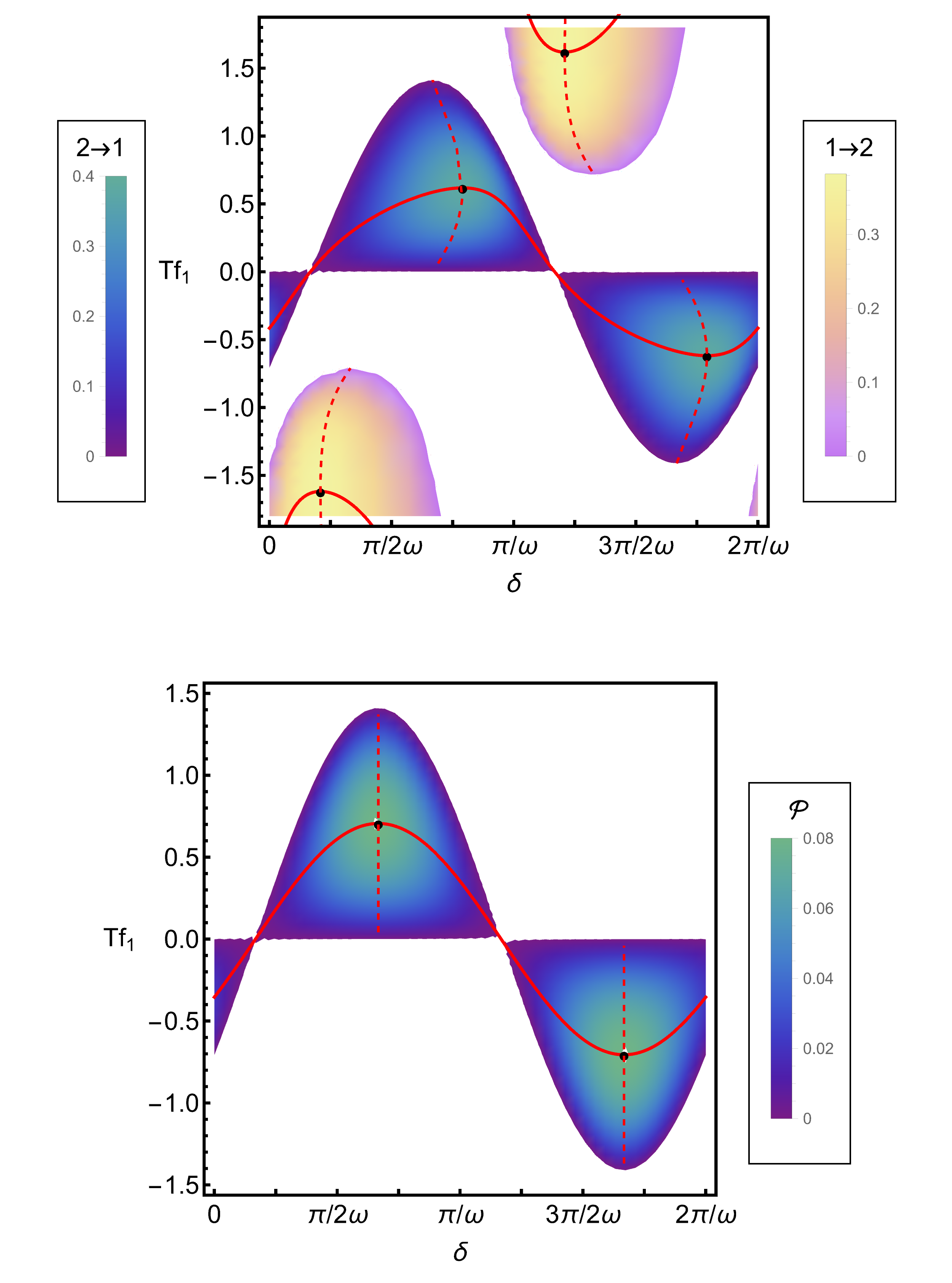
Figure 5: For the same parameters from Fig. 2, depiction of efficiency (top) and power output (bottom) for distinct $Tf_{1}$’s and $\delta$’s. Continuous and dashed lines denote the maximization with respect to the force $f_{1}$ and $\delta$, respectively. The intersection between curves corresponds to the simultaneous maximization (circle).

III.1.3 Complete maximization of engine

Here we address the optimization with respect to the output force and lag simultaneously. In other words, the maximum power output and efficiency must satisfy simultaneously Eqs. (27)/(38) and Eqs. (26)/(39), respectively. Starting with the power output, the existence of an optimal lag $\delta_{mP}^{*}$ and $f_{1mP}^{*}$ imply that

$$\frac{L^{\prime}_{12}(\delta_{mP}^{*})}{L^{\prime}_{11}(\delta_{mP}^{*})}=\frac{1}{2}\frac{L_{12}(\delta_{mP}^{*})}{L_{11}(\delta_{mP}^{*})},$$ (40)

and

$$f_{1mP}^{*}=-\frac{1}{2}\frac{L_{12}(\delta_{mP}^{*})}{L_{11}(\delta_{mP}^{*})}f_{2},$$ (41)

respectively. Expressions for power and efficiency at maximum power at simultaneous maximizations are readily evaluated and given by

$${\cal P}^{*}_{mP}=\frac{T}{4}\frac{L^{2}_{12}(\delta_{mP}^{*})}{L_{11}(\delta_{mP}^{*})}f_{2}^{2},$$ (42)

and

$$\eta^{*}_{mP}=\frac{L^{2}_{12}(\delta_{mP}^{*})}{4L_{11}^{2}(\delta_{mP}^{*})-2L_{12}(\delta_{mP}^{*})L_{21}(\delta_{mP}^{*})}.$$ (43)

Similar expressions for the global maximum efficiency and power at maximum efficiency are obtained by inserting $f_{1mE}^{*}/\delta_{mE}^{*}$ into the expression for power and efficiency, respectively, the former being given by

$$\eta^{*}_{mE}=-\frac{L_{12}(\delta_{mE}^{*})}{L_{21}(\delta_{mE}^{*})}+\frac{2L_{11}^{2}(\delta_{mE}^{*})}{L_{21}^{2}(\delta_{mE}^{*})}\left(1-\sqrt{1-\frac{L_{21}(\delta_{mE}^{*})L_{12}(\delta_{mE}^{*})}{L_{11}^{2}(\delta_{mE}^{*})}}\right),$$ (44)

respectively.

Fig. 5 depicts the simultaneous maximization of power and efficiency with respect to the phase difference and output force for the same parameters from Fig; 2. For the sake of comparison, we also look a the lagless case are depicted in Fig. 1$(a)$ and $(b)$. Although the engine operates rather inefficiently for $\delta=0$ (maximum efficiency and power read $\eta_{mE}\approx 0.172$ and ${\cal P}_{mP}\approx 0.020$) the simultaneous maximization of engine provides a substantial increase of power and output, reading $\eta^{*}_{mE}\approx 0.382$ and ${\cal P}^{*}_{mP}\approx 0.081$. Similar findings are obtained for other values of $\kappa$ and $\omega$, in which the machine performance increases by raising $\kappa$ and lowering $\omega$.

III.2 Different temperatures

In this section, we derive general findings for the case of each particle placed in contact with a distinct thermal bath. We shall restrict our analysis for $k+\kappa>\omega^{2}$, where the efficiency is expected to be larger. Although the power output ${\cal P}$ is the same as before, the efficiency may change due to the appearance of heat flow and therefore its maximization will occur (in general) for distinct output forces and phase differences when compared with the work-to-work converter. The efficiency $\eta$ in such case then reads:

$$\eta=-\frac{{\cal P}}{{\overline{\dot{W}_{\rm 2}}}+{\overline{\dot{Q}_{\rm i}}}}.$$ (45)

Contrasting with the work-to-work converter, in which particles only dump heat to the reservoirs [and hence the heat is not considered in Eq. (25)], the temperature difference may be responsible for some amount of heat flowing from the reservoirs to the system). As the power output is kept the same, the efficiency will always decrease as the temperature gap is raised. For a small difference of temperatures, the heat regime occurs for a lower range of $f_{1}$ or $\delta$ than the entire engine regime, since $Q_{i}\leq 0$ only for some specific parameters. In other words, let $f_{h}$ the threshold force separating both operation regimes (an analogous description holds valid for $\delta_{h}$). For $|f_{h}|<|f_{1}|\leq|f_{m}|$ the engine receives heat from one thermal bath, since $\overline{\dot{Q}}_{i}<0$ or equivalently ${\overline{\kappa}}\Delta T-B_{i}f_{i}f_{j}>A_{i}f_{i}^{2}+C_{i}f_{j}^{2}$. The force $f_{h}$ then satisfies $\overline{\dot{Q}}_{i}(f_{h})=0$, or equivalently $C_{i}f_{h}^{2}+A_{i}f_{i}^{2}={\overline{\kappa}}\Delta T-B_{i}f_{i}f_{h}$. For $0\leq|f_{1}|\leq|f_{h}|$, the machine then works as a work-to-work converter and therefore the temperature difference is playing no role (results from Section III.1 are held valid in this case). It is worth mentioning that above inequality can be satisfied under distinct ways: for large $\Delta T$ and/or choices of $\delta$ or $f_{1}$.

Despite all calculations being exact, expressions for the efficiency and their maximizations become more involved, since they also depend on coefficients $A_{i},B_{i}$ and $C_{i}$. In order to obtain some insights about its behavior in the presence of a heat flux, let us perform an analysis for $\Delta T\ll 1$ and $\Delta T\gg 1$. In the former limit, $\eta$ is approximately given by $\eta\approx-(\overline{\dot{W}}_{1}/\overline{\dot{W}}_{2})(1-\overline{\dot{Q}}_{i}/\overline{\dot{W}}_{2})$. By expressing it in terms of Onsager coefficients, one arrives at the following approximate expression for the efficiency

$$\eta\approx-\frac{L_{11}f_{1}^{2}+L_{12}f_{1}f_{2}}{L_{22}f_{2}^{2}+L_{12}f_{2}f_{1}}\left(1+\frac{\overline{\dot{Q}}_{i}}{T(L_{22}f_{2}^{2}+L_{21}f_{2}f_{1})}\right),$$ (46)

where the input heat $\overline{\dot{Q}}_{i}<0$ plays the role of decreasing the efficiency. Maximizations with respect to $f_{1}$ and $\delta$ can be carried out from above (approximate) expression if $|f_{mE}|\geq|f_{h}|$ and $\delta_{mE}>\delta_{h}$ and from Eq. (26) if $|f_{mE}|\leq|f_{h}|$ and $\delta_{mE}\leq\delta_{h}$.

For the opposite limit $\Delta T\gg 1$, the efficiency is approximately given by $\eta\approx-T(L_{12}f_{1}f_{2}+L_{11}f_{1}^{2})/{\overline{\kappa}}\Delta T$, revealing that $\eta$ decreases asymptotically as $\Delta T^{-1}$ for large temperature differences. Recalling that the numerator does not depend on the temperature (see e.g. Appendix .2), it is clear that $\eta\ll 1$, with maximum values $\eta_{mE}$ and $\eta_{mE,\delta}$ given by $\eta_{mE}\approx{\cal P}_{mP}/{\overline{\kappa}}\Delta T$ and $\eta_{mE,\delta}\approx{\cal P}_{mP,\delta}/{\overline{\kappa}}\Delta T$ for $f_{1mP}$ and $\delta_{mP}$, respectively. For an intermediate $\Delta T$, the system receives heat from the hot thermal bath along $0<|f_{1}|<|f_{m}|$ or $\delta_{m1}\leq\delta\leq\delta_{m2}$, both maximizations are straightforwardly calculated from Eq. (45). Analogous relations are obtained for $T_{i}<T_{j}$ by replacing $\overline{\dot{Q}}_{i}$ for $\overline{\dot{Q}}_{j}$.

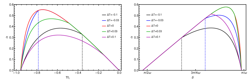
Figure 6: For distinct temperature reservoirs, left and right panels depict the efficiency versus $Tf_{1}$ (for $\delta=0$) and versus $\delta$ (for $Tf_{1}=1$), respectively. The vertical lines denote the values of $f_{h}$ and $\delta_{h}$ separating the operation regimes. The red curves show the work-to-work efficiency. Parameters: $T=0.3+\Delta T/2,\omega=1$, $k=0.1$, $\kappa=5$ and $Tf_{2}=1$.

In order to illustrate above findings, Fig. 6 exemplifies the efficiency for distinct and small $\Delta T=T_{2}-T_{1}$ for fixed $\delta=0$ [left panel] and $f_{1}=1$ [right panel]. As stated before, the power ${\cal P}$ is the same as in Fig. 1$(b)$ for $\kappa=5$. Since $\overline{\dot{Q}}_{1}$ and $\overline{\dot{Q}}_{2}$ exhibit distinct dependencies with $f_{1}$ and $\delta$, the amount of heat received will be different when $\Delta T>0$ or $<0$. Such findings depict that it can more advantageous to receive heat from the thermal bath 1 or 2 depending on the parameters the machine is projected. Such advantages are examined in more details in Fig. 7, in which we extend for lower interaction parameter and several values of $f_{1}$ and $\delta$ for $\Delta T=0.3$ and $-0.3$.

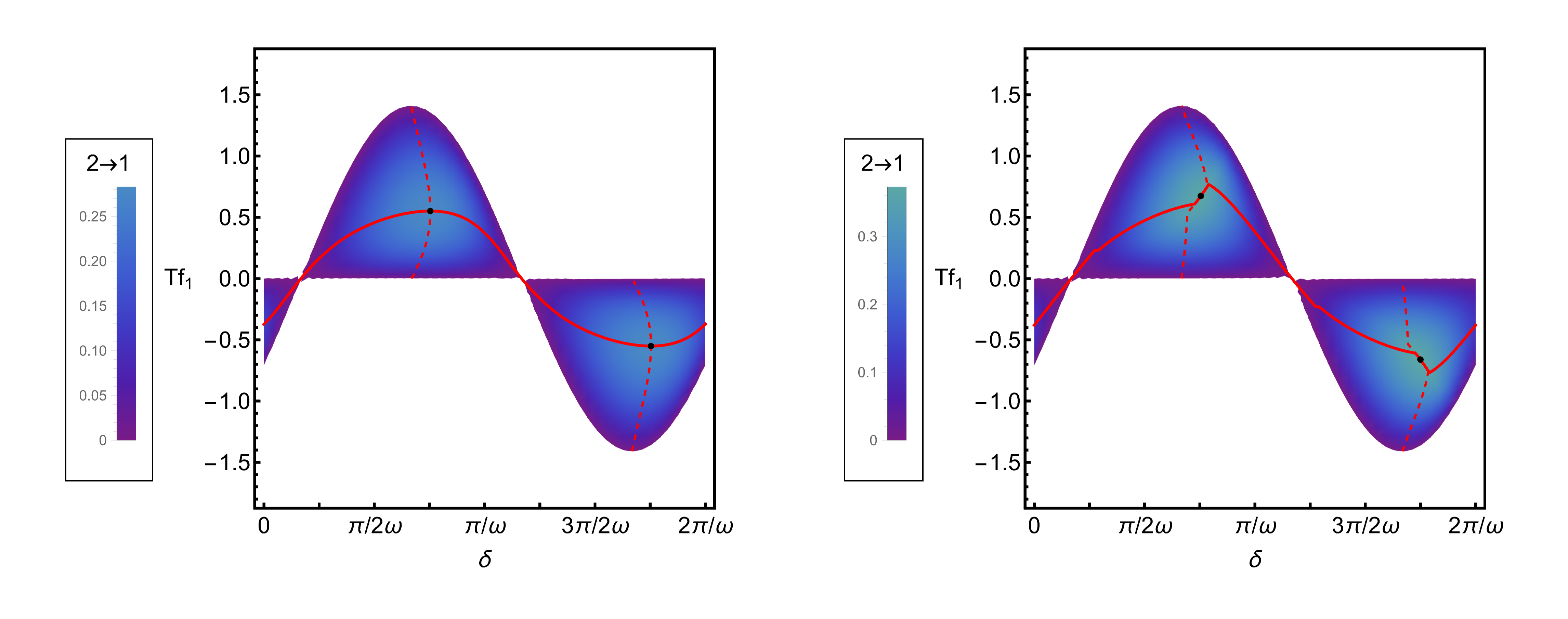
Figure 7: For the same parameters from Fig. 5, left and right panels depict of efficiency (for the conversion from $\overline{\dot{W}}_{2}$ into $\overline{\dot{W}}_{1}$) as a function of $Tf_{1}$ and $\delta$ for $\Delta T=-0.3$ and $0.3$, respectively. Continuous and dashed lines denote the maximization with respect to the force $Tf_{1}$ and $\delta$, respectively. The simultaneous maximization (circles) corresponds to the intersection between maximum curves.

As for the work-to-work converter, there is also the global maximization corresponding to the intersection between both maximum lines. Since the efficiency is lower than the work-to-work converter (see e.g. Fig. 5), the role of the present optimization (whether with respect $f_{1},\delta$ or both) reveals to be relevant for enhancing the engine performance.

IV Conclusions

In this paper, we introduced and analyzed a model for a small scale engine based on interacting Brownian particles subject to periodically driving forces. General expressions for the thermodynamic properties, power output and efficiency were investigated. Interaction between particles plays a central role not only for improving the machine performance but also for changing the machine regime operation. Furthermore, we observe the existence of distinct operation regimes for the same driving strength or phase difference. The present framework reveals to be a suitable route for obtaining efficient thermal engines that benefit from interactions and may constitute a first step for the description of larger chains of interacting particles. It is worth pointing out that positions and velocities get uncoupled for the sort of drivings we have considered and thereby the heat received by the particle can not be converted into useful work. Hence, an interesting extension of the present work would be to exploit other kinds of time dependent drivings providing the heat to be converted into useful work. Another potential extension of our work would be to study engines composed of chains of larger systems sizes, in order to compare the role of system size for enhancing the efficiency and power.

V Acknowledgments

Authors acknowledge financial support from São Paulo Research Foundation (FAPESP) under grants 2020/12021-6, 2017/24567-0, 2020/03708-8 and 2018/02405-1.

Appendix

.1 Expressions for covariances

From the Fokker-Planck-Kramers equation, the time evolution of covariances $b_{ij}^{xv}(t)\equiv\langle x_{i}v_{j}\rangle(t)-\langle x_{i}\rangle(t)\langle v_{j}\rangle(t)$ are given by

$$\frac{db_{11}^{xx}}{dt}=2b_{11}^{xv},$$ (A1)

$$\frac{db_{11}^{vv}}{dt}=-2(k+\kappa)b_{11}^{xv}+2\kappa b_{12}^{xv}-2\gamma b_{11}^{vv}+2\gamma T_{1},$$ (A2)

$$\frac{db_{11}^{xv}}{dt}=b_{11}^{vv}-(k+\kappa)b_{11}^{xx}+\kappa b_{12}^{xx}-\gamma b_{11}^{xv},$$ (A3)

$$\frac{db_{12}^{xx}}{dt}=b_{12}^{xv}+b_{21}^{xv},$$ (A4)

$$\frac{db_{12}^{vv}}{dt}=-(k+\kappa)(b_{12}^{xv}+b_{21}^{xv})+\kappa(b_{11}^{xv}+b_{22}^{xv})-2\gamma b_{12}^{vv},$$ (A5)

and

$$\frac{db_{12}^{xv}}{dt}=b_{12}^{vv}-(k+\kappa)b_{12}^{xx}+\kappa b_{11}^{xx}-\gamma b_{12}^{xv},$$ (A6)

respectively, and analogous relations are obtained for $b_{21}^{xx},b_{21}^{vv},b_{21}^{xv}$ and $b_{22}^{xx},b_{22}^{vv},b_{22}^{xv}$ just by replacing $1\leftrightarrow 2$. From the above set of linear equations, all expressions for steady state covariances are obtained, as listed in Appendix .1. Since only $b_{ij}^{vv}$’s are needed for obtaining the entropy production, we shall omit their expressions, but they can be found in Ref. Tomé and de Oliveira (2010).

.2 Expressions for the entropy production, average work and heat over a complete cycle

In this appendix, we list the main expressions for $\overline{\dot{W}}_{1}$, $\overline{\dot{W}}_{2}$ $\overline{\dot{Q}}_{1}$, $\overline{\dot{Q}}_{2}$ and $\overline{\sigma}$ averaged over a complete cycle. As stated previously, our starting point are the relationships $\dot{W}_{i}=-mF_{i}(t)\expectationvalue{v_{i}}$ and $\dot{Q}_{i}=\gamma\left(m\expectationvalue{v_{i}^{2}}-k_{\text{B}}T_{i}\right)$ together averages $\langle v_{i}\rangle$’s and $\langle v_{i}\rangle^{2}$ integrated over a complete cycle.

The steady state entropy production given by the expression

$$\overline{\sigma}=\frac{\overline{\dot{Q}}_{1}}{T_{1}}+\frac{\overline{\dot{Q}}_{2}}{T_{2}},$$ (A7)

which is a sum of two terms: $\Phi_{T}$ and ${\overline{\Phi}_{f}}$. Such latter one, due to the external forces, has the form $\tilde{L}_{11}X_{1}^{2}+(\tilde{L}_{12}+\tilde{L}_{21})X_{1}X_{2}+\tilde{L}_{22}X_{2}^{2}$, where coefficients (for $m=k_{B}=1$) are given by

$$\tilde{L}_{11}=\frac{\gamma\omega^{2}}{T_{1}T_{2}}\frac{T_{1}\kappa^{2}+T_{2}[(k+\kappa)^{2}+\omega^{2}(\gamma^{2}+\omega^{2}-2(k+\kappa))]}{[\gamma^{2}\omega^{2}+(\omega^{2}-k)^{2}][\gamma^{2}\omega^{2}+(\omega^{2}-k-2\kappa)^{2}]},$$ (A8)

$$\tilde{L}_{12}+\tilde{L}_{21}=\frac{\gamma\omega^{2}\kappa}{2T_{1}T_{2}}\frac{(T_{1}+T_{2})(k+\kappa-\omega^{2})\cos(\delta\omega)+(T_{1}-T_{2})\gamma\omega\sin(\delta\omega)}{[\gamma^{2}\omega^{2}+(\omega^{2}-k)^{2}][\gamma^{2}\omega^{2}+(\omega^{2}-k-2\kappa)^{2}]},$$ (A9)

and

$$\tilde{L}_{22}=\frac{\gamma\omega^{2}}{T_{1}T_{2}}\frac{T_{2}\kappa^{2}+T_{1}[(k+\kappa)^{2}+\omega^{2}(\gamma^{2}+\omega^{2}-2(k+\kappa))]}{[\gamma^{2}\omega^{2}+(\omega^{2}-k)^{2}][\gamma^{2}\omega^{2}+(\omega^{2}-k-2\kappa)^{2}]},$$ (A10)

respectively. Note that above coefficients reduce to Onsager coefficients $L_{21}$’s when $T_{1}=T_{2}$.

In order to relate coefficients ${\tilde{L}}_{ij}$’s with Onsager ones $L_{ij}$’s, it is convenient to expand Eq. (17) in the regime of small $\Delta T$, in such a way that $\overline{\sigma}$ is approximately given by

$$\overline{\sigma}\approx\left[-\frac{1}{T}\left(\overline{\dot{W}}_{1}+\overline{\dot{W}}_{2}\right)+\left(\overline{\dot{Q}}_{1}-\overline{\dot{Q}}_{2}\right)\frac{\Delta T}{2T^{2}}\right].$$ (A11)

Since the dependence with $\Delta T$ is present only in the second right term, it is clear that Onsager coefficients $L_{21}$’s ($i,j\in 1,2$) correspond to 0-th order coefficients obtained from the expansion of $\overline{\sigma}$. For this reason, the coefficient ${\tilde{L}}_{ij}$ can be decomposed as ${\tilde{L}}_{ij}=L_{ij}+L_{ij}^{(c)}\Delta T$, where $L_{ij}^{(c)}$ is the first order correction and then $\overline{\sigma}$ is given by

$$\begin{split}\overline{\sigma}&\approx L_{11}f_{1}^{2}+\left(L_{12}+L_{21}\right)f_{1}f_{2}+L_{22}f_{2}^{2}+\\ &\left[L_{11}^{(c)}f_{1}^{2}+\left(L_{12}^{(c)}+L_{21}^{(c)}\right)f_{1}f_{2}+L_{22}^{(c)}f_{2}^{2}\right]\Delta T+L_{TT}f_{T}^{2},\end{split}$$ (A12)

where $L_{TT}=\overline{\kappa}T^{2}>0$ with $f_{1}=X_{1}/T$, $f_{2}=X_{2}/T$ and $f_{T}=\Delta T/T^{2}$ [where $T=(T_{1}+T_{2})/2$]. As analyzed in Sec. II, for small $\Delta T$ and $f_{i}$’s, the difference between $L_{ij}$’s and ${\tilde{L}}_{ij}$’s can be neglected and the entropy production is approximately given by $\overline{\sigma}\approx L_{11}f_{1}^{2}+\left(L_{12}+L_{21}\right)f_{1}f_{2}+L_{22}f_{2}^{2}+L_{TT}f_{T}^{2}$.

The averaged expressions for $\overline{\dot{W}}_{1}$, $\overline{\dot{W}}_{2}$, $\overline{\dot{Q}}_{1}$ and $\overline{\dot{Q}}_{2}$ are given by

$$\overline{\dot{W}}_{1} =-\frac{T^{2}\gamma\omega^{2}\left(\gamma^{2}\omega^{2}+\left(\omega^{2}-(k+\kappa)\right)^{2}+\kappa^{2}\right)}{2\left[\gamma^{2}\omega^{2}+\left(\omega^{2}-k\right)^{2}\right]\left[\gamma^{2}\omega^{2}+(\omega^{2}-(k+2\kappa))^{2}\right]}f_{1}^{2}$$

$$-\frac{T^{2}\kappa\omega}{2}\frac{2\gamma\omega\left(\kappa+k-\omega^{2}\right)\cos(\delta\omega)-\sin(\delta\omega)\left[\gamma^{2}\omega^{2}-(\omega^{2}-(k+\kappa))^{2}+\kappa^{2}\right]}{\left[\gamma^{2}\omega^{2}+\left(\omega^{2}-k\right)^{2}\right]\left[\gamma^{2}\omega^{2}+(\omega^{2}-(k+2\kappa))^{2}\right]}f_{1}f_{2},$$ (A13)

$$\overline{\dot{W}}_{2} =-\frac{T^{2}\gamma\omega^{2}\left(\gamma^{2}\omega^{2}+\left(\omega^{2}-(k+\kappa)\right)^{2}+\kappa^{2}\right)}{2\left[\gamma^{2}\omega^{2}+\left(\omega^{2}-k\right)^{2}\right]\left[\gamma^{2}\omega^{2}+(\omega^{2}-(k+2\kappa))^{2}\right]}f_{2}^{2}$$

$$-\frac{T^{2}\kappa\omega}{2}\frac{2\gamma\omega\left(\kappa+k-\omega^{2}\right)\cos(\delta\omega)+\sin(\delta\omega)\left[\gamma^{2}\omega^{2}-(\omega^{2}-(k+\kappa))^{2}+\kappa^{2}\right]}{\left[\gamma^{2}\omega^{2}+\left(\omega^{2}-k\right)^{2}\right]\left[\gamma^{2}\omega^{2}+(\omega^{2}-(k+2\kappa))^{2}\right]}f_{1}f_{2},$$ (A14)

where

$$\centering\overline{\dot{Q}}_{1}\@add@centering =\frac{T^{2}\gamma\omega^{2}\left[\gamma^{2}\omega^{2}+\left(\kappa+k-\omega^{2}\right)^{2}\right]}{2\left[\gamma^{2}\omega^{2}+\left(k-\omega^{2}\right)^{2}\right]\left[\gamma^{2}\omega^{2}+\left(2\kappa+k-\omega^{2}\right)^{2}\right]}f_{1}^{2}+\frac{T^{2}\gamma\kappa^{2}\omega^{2}}{2\left[\gamma^{2}\omega^{2}+\left(k-\omega^{2}\right)^{2}\right]\left[\gamma^{2}\omega^{2}+\left(2\kappa+k-\omega^{2}\right)^{2}\right]}f_{2}^{2}$$

$$+\frac{T^{2}\gamma\kappa\omega^{2}\left[\cos(\delta\omega)\left(\kappa+k-\omega^{2}\right)-\gamma\omega\sin(\delta\omega)\right]}{\left[\gamma^{2}\omega^{2}+\left(k-\omega^{2}\right)^{2}\right]\left[\gamma^{2}\omega^{2}+\left(2\kappa+k-\omega^{2}\right)^{2}\right]}f_{1}f_{2}+\frac{\gamma\kappa^{2}}{2[\gamma^{2}k+\kappa\left(\kappa+\gamma^{2}\right)]}\Delta T$$ (A15)

and

$$\centering\overline{\dot{Q}}_{2}\@add@centering =\frac{T^{2}\gamma\kappa^{2}\omega^{2}}{2\left[\gamma^{2}\omega^{2}+\left(k-\omega^{2}\right)^{2}\right]\left[\gamma^{2}\omega^{2}+\left(2\kappa+k-\omega^{2}\right)^{2}\right]}f_{1}^{2}+\frac{T^{2}\gamma\omega^{2}\left[\gamma^{2}\omega^{2}+\left(\kappa+k-\omega^{2}\right)^{2}\right]}{2\left[\gamma^{2}\omega^{2}+\left(k-\omega^{2}\right)^{2}\right]\left[\gamma^{2}\omega^{2}+\left(2\kappa+k-\omega^{2}\right)^{2}\right]}f_{2}^{2}$$

$$+\frac{T^{2}\gamma\kappa\omega^{2}\left[\cos(\delta\omega)\left(\kappa+k-\omega^{2}\right)+\gamma\omega\sin(\delta\omega)\right]}{\left[\gamma^{2}\omega^{2}+\left(k-\omega^{2}\right)^{2}\right]\left[\gamma^{2}\omega^{2}+\left(2\kappa+k-\omega^{2}\right)^{2}\right]}f_{1}f_{2}-\frac{\gamma\kappa^{2}}{2\left[\gamma^{2}k+\kappa\left(\kappa+\gamma^{2}\right)\right]}\Delta T$$ (A16)

respectively.

References

• Seifert (2012) U. Seifert, Reports on progress in physics 75, 126001 (2012).
• Liepelt and Lipowsky (2007) S. Liepelt and R. Lipowsky, Phys. Rev. Lett. 98, 258102 (2007).
• Liepelt and Lipowsky (2009) S. Liepelt and R. Lipowsky, Phys. Rev. E 79, 011917 (2009).
• Crooks (1999) G. E. Crooks, Phys. Rev. E 60, 2721 (1999).
• Jarzynski (1997) C. Jarzynski, Phys. Rev. Lett. 78, 2690 (1997).
• Barato and Seifert (2015) A. C. Barato and U. Seifert, Physical review letters 114, 158101 (2015).
• Pietzonka et al. (2016) P. Pietzonka, A. C. Barato,  and U. Seifert, Physical Review E 93, 052145 (2016).
• Barato et al. (2018) A. C. Barato, R. Chetrite, A. Faggionato,  and D. Gabrielli, New Journal of Physics 20, 103023 (2018).
• Barato et al. (2019) A. Barato, R. Chetrite, A. Faggionato,  and D. Gabrielli, Journal of Statistical Mechanics: Theory and Experiment 2019, 084017 (2019).
• Proesmans and Van den Broeck (2017a) K. Proesmans and C. Van den Broeck, EPL (Europhysics Letters) 119, 20001 (2017a).
• Harunari et al. (2020) P. E. Harunari, C. E. Fiore,  and K. Proesmans, Journal of Physics A: Mathematical and Theoretical 53, 374001 (2020).
• Hasegawa and Van Vu (2019) Y. Hasegawa and T. Van Vu, Phys. Rev. E 99, 062126 (2019).
• Van Vu and Hasegawa (2020) T. Van Vu and Y. Hasegawa, Phys. Rev. Research 2, 013060 (2020).
• Pietzonka and Seifert (2018) P. Pietzonka and U. Seifert, Phys. Rev. Lett. 120, 190602 (2018).
• Martínez et al. (2016) I. A. Martínez, É. Roldán, L. Dinis, D. Petrov, J. M. Parrondo,  and R. A. Rica, Nature physics 12, 67 (2016).
• Krishnamurthy et al. (2016) S. Krishnamurthy, S. Ghosh, D. Chatterji, R. Ganapathy,  and A. Sood, Nature Physics 12, 1134 (2016).
• Blickle and Bechinger (2012) V. Blickle and C. Bechinger, Nature Physics 8, 143 (2012).
• Proesmans et al. (2016a) K. Proesmans, Y. Dreher, M. Gavrilov, J. Bechhoefer,  and C. Van den Broeck, Physical Review X 6, 041010 (2016a).
• Quinto-Su (2014) P. A. Quinto-Su, Nature communications 5, 1 (2014).
• Jones et al. (2015) P. H. Jones, O. M. Maragò,  and G. Volpe, Optical tweezers: Principles and applications (Cambridge University Press, 2015).
• Albay et al. (2018) J. A. Albay, G. Paneru, H. K. Pak,  and Y. Jun, Optics express 26, 29906 (2018).
• Kumar and Bechhoefer (2018) A. Kumar and J. Bechhoefer, Applied Physics Letters 113, 183702 (2018).
• Paneru and Kyu Pak (2020) G. Paneru and H. Kyu Pak, Advances in Physics: X 5, 1823880 (2020).
• Li et al. (2019) J. Li, J. M. Horowitz, T. R. Gingrich,  and N. Fakhri, Nature communications 10, 1 (2019).
• Noa et al. (2020) C. F. Noa, W. G. Oropesa,  and C. Fiore, Physical Review Research 2, 043016 (2020).
• Proesmans et al. (2015) K. Proesmans, C. Driesen, B. Cleuren,  and C. Van den Broeck, Physical review E 92, 032105 (2015).
• Rana et al. (2014) S. Rana, P. Pal, A. Saha,  and A. Jayannavar, Physical review E 90, 042146 (2014).
• Schmiedl and Seifert (2007) T. Schmiedl and U. Seifert, EPL (Europhysics Letters) 81, 20003 (2007).
• Hoppenau et al. (2013) J. Hoppenau, M. Niemann,  and A. Engel, Physical Review E 87, 062127 (2013).
• Tu (2014) Z. Tu, Physical Review E 89, 052148 (2014).
• Chvosta et al. (2010) P. Chvosta, M. Einax, V. Holubec, A. Ryabov,  and P. Maass, Journal of Statistical Mechanics: Theory and Experiment 2010, P03002 (2010).
• Verley et al. (2014) G. Verley, M. Esposito, T. Willaert,  and C. Van den Broeck, Nature communications 5, 1 (2014).
• Imparato et al. (2007) A. Imparato, L. Peliti, G. Pesce, G. Rusciano,  and A. Sasso, Physical Review E 76, 050101 (2007).
• Plata et al. (2020) C. A. Plata, D. Guéry-Odelin, E. Trizac,  and A. Prados, Journal of Statistical Mechanics: Theory and Experiment 2020, 093207 (2020).
• Albay et al. (2021) J. A. Albay, Z.-Y. Zhou, C.-H. Chang,  and Y. Jun, Scientific reports 11, 1 (2021).
• Jun et al. (2014) Y. Jun, M. Gavrilov,  and J. Bechhoefer, Physical review letters 113, 190601 (2014).
• Park et al. (2016) J.-M. Park, H.-M. Chun,  and J. D. Noh, Physical Review E 94, 012127 (2016).
• Akasaki et al. (2020) B. A. Akasaki, M. J. de Oliveira,  and C. E. Fiore, Physical Review E 101, 012132 (2020).
• Curzon and Ahlborn (1975) F. Curzon and B. Ahlborn, American Journal of Physics 43, 22 (1975).
• Holubec (2014) V. Holubec, Journal of Statistical Mechanics: Theory and Experiment 2014, P05022 (2014).
• Harunari et al. (2021) P. E. Harunari, F. S. Filho, C. E. Fiore,  and A. Rosas, Phys. Rev. Research 3, 023194 (2021).
• Golubeva and Imparato (2012) N. Golubeva and A. Imparato, Phys. Rev. Lett. 109, 190602 (2012).
• Proesmans and Van den Broeck (2017b) K. Proesmans and C. Van den Broeck, Chaos: An Interdisciplinary Journal of Nonlinear Science 27, 104601 (2017b).
• Tomé and de Oliveira (2010) T. Tomé and M. J. de Oliveira, Physical Review E 82, 021120 (2010).
• Van den Broeck and Esposito (2010) C. Van den Broeck and M. Esposito, Phys. Rev. E 82, 011144 (2010).
• Fiore and de Oliveira (2019) C. E. Fiore and M. J. de Oliveira, Phys. Rev. E 99, 052131 (2019).
• Morgado and Soares-Pinto (2009) W. A. M. Morgado and D. O. Soares-Pinto, Phys. Rev. E 79, 051116 (2009).
• de Oliveira et al. (2021) J. L. D. de Oliveira, M. Rojas,  and C. Filgueiras, Phys. Rev. E 104, 014149 (2021).
• Huang et al. (2014) X.-L. Huang, X.-Y. Niu, X.-M. Xiu,  and X.-X. Yi, The European Physical Journal D 68, 1 (2014).
• Proesmans et al. (2016b) K. Proesmans, B. Cleuren,  and C. Van den Broeck, Physical review letters 116, 220601 (2016b).