Structured vector fitting framework for mechanical systems

Abstract

In this paper, we develop a structure-preserving formulation of the data-driven vector fitting algorithm for the case of modally damped mechanical systems. Using the structured pole-residue form of the transfer function of modally damped second-order systems, we propose two possible structured extensions of the barycentric formula of system transfer functions. Integrating these new forms within the classical vector fitting algorithm leads to the formulation of two new algorithms that allow the computation of modally damped mechanical systems from data in a least squares fashion. Thus, the learned model is guaranteed to have the desired structure. We test the proposed algorithms on two benchmark models.

1 Introduction

Data-driven reduced-order modeling (DD-ROM) is essential in constructing high-fidelity compact models to approximate the underlying physical phenomena when an explicit model, a state-space formulation with access to internal variables, is not available yet an abundant input/output data is. Thus, DD-ROM circumvents the need to access an exact description of the original model and is applicable when traditional intrusive projection-based model reduction is not. As in the projection case, it is important that the learned model inherits the physical meaning and structures of the system that has generated the data. This is the setup we are interested in here. Our goal is to develop a data-driven structure-preserving modeling framework for mechanical systems described by second-order dynamics.

Data in our setting will correspond to transfer function (frequency domain) samples of the underlying mechanical system. Let $H(s)$ denote this transfer function and let $\xi_{k}$ denote the sampling frequencies (points). Thus, we assume access to the data (measurements) $h_{k}=H(\xi_{k})$, for $k=1,2,\dots,\ell$. The goal of DD-ROM in this setting is to construct a reduced transfer function (a low-order rational function) ${\hstretch{2}{\hat{\hstretch{.5}{H\mkern 4.0mu}}}\mkern-4.0mu}{}(s)$ such that ${\hstretch{2}{\hat{\hstretch{.5}{H\mkern 4.0mu}}}\mkern-4.0mu}{}(\xi_{k})\approx h_{k}=H(\xi_{k})$ in an appropriate measure. We will call this unstructured (or first-order fitting in this paper) since the only requirement in this case is that ${\hstretch{2}{\hat{\hstretch{.5}{H\mkern 4.0mu}}}\mkern-4.0mu}{}(s)$ is a rational function and thus corresponds to a transfer function with a first-order state-space form. In this setting, the barycentric rational form of the approximant plays a crucial role; see [4]. The Loewner framework from [1, 9] that enforces interpolation of the data, the Vector Fitting (VF) algorithm from [8] that minimizes a least-squares distance, and the AAA algorithm from [10] that combines interpolation and least squares are just three of the many techniques for rational data fitting. We refer the reader to [12, Sec. 2.1] for further references.

Second‐order systems are an important class of structured dynamical systems used to describe, for example, the dynamics of mechanical systems, and in particular, their vibrational response. Since the underlying second-order structure corresponds to important physical properties, retaining this structure is vital so that the learned model is physically meaningful. Therefor, given the frequency response samples of such systems, our goal is to construct a structure-preserving DD-ROM, in the sense that the learned model can be interpreted as the transfer function of a second-order (mechanical) system. Note that not every rational function can be written as the transfer function of a second-order system (although the reverse is true). There have been some recent works on constructing data-driven second-order models in the interpolatory Loewner framework; see [15, 3]. There is a much wider literature on projection-based structure-preserving model reduction for second-order systems. We refer the reader to [13, 17] and the references therein for details on the projection-based approaches that we do not consider here.

In this paper, we will focus on structure-preserving second-order DD-ROM using the least-squares measure. More specifically, we will enforce modal-damping structure in the learned model. We will achieve this goal by extending the VF algorithm to the structured setting. Up to now, VF has been developed to produce unstructured rational approximants. We will revise the barycentric formula behind the VF approximant such that upon convergence the learned model has the desired second-order structure. This new formulation of the barycentric form will lead to a sequence of linear least-squares problems whose structure will also inherit the underlying second-order dynamics.

The rest of the paper is organized as follows: After providing an overview of the classical VF approach and modally damped second-order systems in Section 2, we develop the modified barycentric forms and the resulting structure-preserving VF approaches together with the corresponding proposed numerical algorithms in Section 3. The proposed methods are then tested on two benchmark examples in Section 4, followed by the conclusions and future research directions in Section 5.

2 Background

In this section, we provide a brief overview of the classical vector fitting algorithm and summarize the key structural features of the special class of mechanical systems under consideration.

2.1 Classical vector fitting approach

Assume that one has access to the samples of the transfer function of an underlying single-input/single-output (SISO) dynamical system to be modeled, $H(s)$, at the sampling points (frequencies) $\xi_{1},\xi_{2},\ldots,\xi_{\ell}\in\mathbb{C}$. Given the data $\{H(\xi_{i})\}_{i=1}^{\ell}$, the goal is to construct (learn) a degree-$r$ scalar rational function ${\hstretch{2}{\hat{\hstretch{.5}{H\mkern 4.0mu}}}\mkern-4.0mu}{}(s)$ to solve the nonlinear rational least-squares (LS) problem

$$\min\limits_{{\hstretch{2}{\hat{\hstretch{.5}{H\mkern 4.0mu}}}\mkern-4.0mu}{}}\sum\limits_{i=1}^{\ell}\lvert{\hstretch{2}{\hat{\hstretch{.5}{H\mkern 4.0mu}}}\mkern-4.0mu}{}(\xi_{k})-H(\xi_{k})\rvert^{2}.$$ (1)

Let ${\hstretch{2}{\hat{\hstretch{.5}{H\mkern 4.0mu}}}\mkern-4.0mu}{}(s)=\frac{n(s)}{d(s)}$ where $n(s)$ and $d(s)$ are, respectively, degree-$(r-1)$ and degree-$r$ polynomials in $s$. In other words, $H(s)$ is parametrized by its denominator and numerator coefficients. Inserting this form of ${\hstretch{2}{\hat{\hstretch{.5}{H\mkern 4.0mu}}}\mkern-4.0mu}{}(s)$ into Eq. 1, one can re-write the nonlinear LS error to minimize as

$$\sum\limits_{i=1}^{\ell}\lvert{\hstretch{2}{\hat{\hstretch{.5}{H\mkern 4.0mu}}}\mkern-4.0mu}{}(\xi_{i})-H(\xi_{i})\rvert^{2} =\sum\limits_{i=1}^{\ell}\frac{1}{\lvert d(\xi_{i})\rvert^{2}}\lvert n(\xi_{i})-d(\xi_{i})H(\xi_{i})\rvert^{2}.$$

The nonlinearity results from the nonlinear dependence of the error on $d(s)$. To solve this nonlinear LS problem, starting with an initial guess of ${\hstretch{2}{\hat{\hstretch{.5}{H\mkern 4.0mu}}}\mkern-4.0mu}{}^{(0)}(s)=\frac{d^{(0)}(s)}{n^{(0)}(s)}$, [14] proposed an iterative scheme where in the $k$-th step the error term Eq. 1 is replaced by

$$\begin{aligned} \sum\limits_{i=1}^{\ell}\lvert{\hstretch{2}{\hat{\hstretch{.5}{H\mkern 4.0mu}}}\mkern-4.0mu}{}^{(k)}(\xi_{i})-H(\xi_{i})\rvert^{2}&=\\ \sum\limits_{i=1}^{\ell}\frac{1}{\lvert d^{(k-1)}(\xi_{i})\rvert^{2}}&\lvert n^{(k)}(\xi_{i})-d^{(k)}(\xi_{i})H(\xi_{i})\rvert^{2}.\end{aligned}$$ (2)

Note that the new error term Eq. 2 is now linear in the variables $n^{(k)}$ and $d^{(k)}(s)$. Therefor, the SK iteration in [14] converts the original nonlinear LS problem Eq. 1 into solving a sequence of weighted linear LS problems Eq. 2.

There are various equivalent forms to represent the rational function ${\hstretch{2}{\hat{\hstretch{.5}{H\mkern 4.0mu}}}\mkern-4.0mu}{}(s)$. One can work with numerator and denominator coefficients as the unknowns, or the poles and residues, for example. A numerically efficient formulation is the so-called barycentric representation; see [4]. Let ${\hstretch{2}{\hat{\hstretch{.5}{H\mkern 4.0mu}}}\mkern-4.0mu}{}^{(k)}(s)$ denote the iterate in the $k$-th step of the SK iteration as above. Also let $\lambda_{1}^{(k)},\ldots,\lambda_{r}^{(k)}$ be mutually distinct points. Then, ${\hstretch{2}{\hat{\hstretch{.5}{H\mkern 4.0mu}}}\mkern-4.0mu}{}^{(k)}(s)$ can be written in the barycentric form as

$${\hstretch{2}{\hat{\hstretch{.5}{H\mkern 4.0mu}}}\mkern-4.0mu}{}^{(k)}(s) =\frac{n^{(k)}(s)}{d^{(k)}(s)}=\frac{\sum\limits_{j=1}^{r}\frac{\phi^{(k)}_{j}}{s-\lambda^{(k)}_{j}}}{1+\sum\limits_{j=1}^{r}\frac{\varphi^{(k)}_{j}}{s-\lambda^{(k)}_{j}}},$$ (3)

where $\{\phi_{j}^{(k)}\}_{j=1}^{r}$ and $\{\varphi_{j}^{(k)}\}_{j=1}^{r}$ are the barycentric weights. Note that the $\lambda_{j}^{(k)}$’s are not the poles of ${\hstretch{2}{\hat{\hstretch{.5}{H\mkern 4.0mu}}}\mkern-4.0mu}{}(s)$. We refer the reader to, e.g., [6] to switch between the pole-residue form and the barycentric form.

Now inserting $n^{(k)}(s)$ and $d^{(k)}(s)$ from Eq. 3 into Eq. 2, in the $k$-th step of the SK iteration, one needs to solve the weighted linear LS problem

$$\min\limits_{x^{(k)}}\lVert\Delta^{(k)}(A^{(k)}x^{(k)}-h)\rVert_{2}^{2},$$ (4)

where

$$\Delta^{(k)} =\operatorname{diag}\left(\frac{1}{\lvert d^{(k)}(\xi_{1})\rvert},\ldots,\frac{1}{\lvert d^{(k)}(\xi_{\ell})\rvert}\right),\quad h=\begin{bmatrix}H(\xi_{1})\\ \vdots\\ H(\xi_{\ell})\end{bmatrix},$$ (5)

$$A^{(k)} =\begin{bmatrix}\frac{1}{\xi_{1}-\lambda_{1}^{(k)}}&\cdots&\frac{1}{\xi_{1}-\lambda_{r}^{(k)}}&\frac{-H(\xi_{1})}{\xi_{1}-\lambda_{1}^{(k)}}&\cdots&\frac{-H(\xi_{1})}{\xi_{1}-\lambda_{r}^{(k)}}\\ \vdots&&\vdots&\vdots&&\vdots\\ \frac{1}{\xi_{\ell}-\lambda_{1}^{(k)}}&\cdots&\frac{1}{\xi_{\ell}-\lambda_{r}^{(k)}}&\frac{-H(\xi_{\ell})}{\xi_{\ell}-\lambda_{1}^{(k)}}&\cdots&\frac{-H(\xi_{\ell})}{\xi_{\ell}-\lambda_{r}^{(k)}}\end{bmatrix},$$ (6)

for the solution vector

$$x^{(k)} =\begin{bmatrix}\phi_{1}^{(k)}&\cdots&\phi_{r}^{(k)}&\varphi_{1}^{(k)}&\cdots&\varphi_{r}^{(k)}\end{bmatrix}^{\mkern-1.5mu\mathsf{T}},$$

which forms ${\hstretch{2}{\hat{\hstretch{.5}{H\mkern 4.0mu}}}\mkern-4.0mu}{}^{(k)}(s)$ at the $k$-th step. In addition to incorporating the barycentric form into the SK iterations, [8] have also observed that the only restrictions on $\{\lambda_{j}^{(k)}\}_{j=1}^{r}$ is to be distinct and they can be updated at every step. This is precisely what [8] have proposed, leading to the Vector Fitting (VF) algorithm. VF updates $\{\lambda_{j}^{(k)}\}_{j=1}^{r}$ as the roots of denominator $d^{(k)}(s)$. Making again use of the barycentric representation Eq. 3, these roots are actually the eigenvalues of ${\hstretch{2}{\hat{\hstretch{.5}{A\mkern 4.0mu}}}\mkern-4.0mu}{}^{(k)}-{\hstretch{2}{\hat{\hstretch{.5}{G\mkern 4.0mu}}}\mkern-4.0mu}{}^{(k)}{\hstretch{2}{\hat{\hstretch{.5}{C\mkern 4.0mu}}}\mkern-4.0mu}{}^{(k)}$, where

$${\hstretch{2}{\hat{\hstretch{.5}{A\mkern 4.0mu}}}\mkern-4.0mu}{}^{(k)} =\operatorname{diag}(\lambda_{1}^{(k)},\ldots,\lambda_{r}^{(k)}),$$ (7)

$${\hstretch{2}{\hat{\hstretch{.5}{G\mkern 4.0mu}}}\mkern-4.0mu}{}^{(k)} =\begin{bmatrix}\varphi_{1}^{(k)}\leavevmode\nobreak\ \ldots\leavevmode\nobreak\ \varphi_{r}^{(k)}\end{bmatrix}^{\mkern-1.5mu\mathsf{T}}\leavevmode\nobreak\ \leavevmode\nobreak\ \text{and}\leavevmode\nobreak\ \leavevmode\nobreak\ {\hstretch{2}{\hat{\hstretch{.5}{C\mkern 4.0mu}}}\mkern-4.0mu}{}^{(k)}=\begin{bmatrix}1\leavevmode\nobreak\ \ldots\leavevmode\nobreak\ 1\end{bmatrix}^{\mkern-1.5mu\mathsf{T}}.$$ (8)

If the algorithm converges, due to the $\{\lambda_{j}^{(k)}\}_{j=1}^{r}$ updating strategy, $d^{(k)}(s)\to 1$ and thus the final approximation is obtained in the pole-residue form with the denominator being $1$ in Eq. 3. The resulting method is summarized in Algorithm 1, and we refer the reader to [8], [7, Chap7] and [5] for further details.

Algorithm 1 (Unstructured) Vector Fitting (VF)

Input: Vector $h$ of data samples Eq. 5, initial guess for

Input: $\{\lambda_{j}^{(1)}\}_{j=1}^{r}$.
      Output: Learned ROM ${\hstretch{2}{\hat{\hstretch{.5}{H\mkern 4.0mu}}}\mkern-4.0mu}{}(s)={\hstretch{2}{\hat{\hstretch{.5}{C\mkern 4.0mu}}}\mkern-4.0mu}{}(sI_{r}-{\hstretch{2}{\hat{\hstretch{.5}{A\mkern 4.0mu}}}\mkern-4.0mu}{})^{-1}{\hstretch{2}{\hat{\hstretch{.5}{B\mkern 4.0mu}}}\mkern-4.0mu}{}$.

1:Initialize $\Delta^{(1)}=I_{\ell}$ and $k=1$.

2:while not converged do

3:   Construct the coefficient matrix $A^{(k)}$ in Eq. 6.

4:   Solve the weighted linear least-squares problem Eq. 4.

5:   Update the expansion points $\{\lambda_{j}^{(k+1)}\}_{j=1}^{r}$ to be the eigenvalues of ${\hstretch{2}{\hat{\hstretch{.5}{A\mkern 4.0mu}}}\mkern-4.0mu}{}^{(k)}-{\hstretch{2}{\hat{\hstretch{.5}{G\mkern 4.0mu}}}\mkern-4.0mu}{}^{(k)}{\hstretch{2}{\hat{\hstretch{.5}{C\mkern 4.0mu}}}\mkern-4.0mu}{}^{(k)}$ using Eq. 7 and Eq. 8.

6:   Update the weighting matrix $\Delta^{(k+1)}$ by Eq. 5.

7:   Increment $k\leftarrow k+1$.

8:end while

9:Set the final ROM matrices to be ${\hstretch{2}{\hat{\hstretch{.5}{A\mkern 4.0mu}}}\mkern-4.0mu}{}=\operatorname{diag}(\lambda_{1}^{(k)},\ldots,\lambda_{r}^{(k)})$, ${\hstretch{2}{\hat{\hstretch{.5}{B\mkern 4.0mu}}}\mkern-4.0mu}{}=\begin{bmatrix}\phi_{1}^{(k)}&\ldots&\phi_{r}^{(k)}\end{bmatrix}^{\mkern-1.5mu\mathsf{T}}$ and ${\hstretch{2}{\hat{\hstretch{.5}{C\mkern 4.0mu}}}\mkern-4.0mu}{}=\begin{bmatrix}1&\ldots&1\end{bmatrix}^{\mkern-1.5mu\mathsf{T}}$.

2.2 Modally damped second-order systems

Next, we take a look at the pole-residue formulation of the structured system class we consider here, namely the modally damped second-order systems. As in the previous section, for simplicity we restrict the analysis to the SISO case. Assume we have a second-order system of the form

$$\begin{aligned} M\ddot{q}(t)+E\dot{q}(t)+Kq(t)&=B_{\mathrm{u}}u(t),\\ y(t)&=C_{\mathrm{p}}q(t),\end{aligned}$$

with $M,E,K\in\mathbb{R}^{n\times n}$, $B_{\mathrm{u}}\in\mathbb{R}^{n}$, $C_{\mathrm{p}}^{\mkern-1.5mu\mathsf{T}}\in\mathbb{R}^{n}$, and modal damping $EM^{-1}K=KM^{-1}E$ as in [2]. Note here that for the mechanical system case one additionally has $M=M^{\mkern-1.5mu\mathsf{T}}>0$, $E=E^{\mkern-1.5mu\mathsf{T}}\geq 0$, and $K=K^{\mkern-1.5mu\mathsf{T}}>0$. This assumption is not necessary in general and instead we only assume that the pencil $\lambda M-K$ is diagonalizable, since with modal damping all three system matrices are simultaneously diagonalizable. First, we consider the generalized eigenvalue problems

$$\begin{aligned} KX&=MX\Omega^{2},&K^{\mkern-1.5mu\mathsf{T}}Y&=M^{\mkern-1.5mu\mathsf{T}}Y\Omega^{2},\end{aligned}$$

where the eigenvector matrices $X$ and $Y$ are scaled such that

$$\begin{aligned} Y^{\mkern-1.5mu\mathsf{T}}MX&=\Omega^{-1},&Y^{\mkern-1.5mu\mathsf{T}}KX&=\Omega,\end{aligned}$$

with $\Omega=\operatorname{diag}(\omega_{1},\ldots,\omega_{n})$. Due to modal damping, the damping matrix can also be diagonalized such that

$$Y^{\mkern-1.5mu\mathsf{T}}EX =2\Psi,$$

where $\Psi=\operatorname{diag}(\psi_{1},\ldots,\psi_{n})$ are the damping ratios of the system. Then, the transfer function $H(s)$ satisfies

$$H(s) =C_{\mathrm{p}}(s^{2}M+sE+K)^{-1}B_{\mathrm{u}}$$

$$=C_{\mathrm{p}}X(s^{2}\Omega^{-1}+2s\Psi+\Omega)^{-1}Y^{\mkern-1.5mu\mathsf{T}}B_{\mathrm{u}}$$

$$=\sum\limits_{j=1}^{n}\frac{\omega_{j}\phi^{\pm}_{j}}{s^{2}+2\psi_{j}\omega_{j}s+\omega_{j}^{2}}$$

$$=\sum\limits_{j=1}^{n}\frac{\omega_{j}\phi^{\pm}_{j}}{(s-\lambda_{j}^{+})(s-\lambda_{j}^{-})},$$ (9)

where the pairwise poles of the system are given by

$$\lambda^{\pm}_{j} =-\omega_{j}\psi_{j}\pm\omega_{j}\sqrt{\psi_{j}^{2}-1}.$$ (10)

Since every second-order system can also be written in its first-order form, we can also write $H(s)$ in the generic pole-residue formulation as

$$H(s) =\sum\limits_{j=1}^{2n}\frac{\phi_{j}}{s-\lambda_{j}}=\sum\limits_{j=1}^{n}\frac{\phi_{j}^{+}}{s-\lambda_{j}^{+}}+\sum\limits_{j=1}^{n}\frac{\phi_{j}^{-}}{s-\lambda_{j}^{-}}.$$ (11)

Note that modal damping and the second-order structure enforce additional properties in the generic pole-residue form, which means that only for the underlying second-order systems those two formulations, i.e., Eq. 9 and Eq. 11, are equivalent. A clear and important advantage of Eq. 9 is the enforcement of the underlying system structure.

$$A_{\mathrm{so1}}^{(k)} =\begin{bmatrix}\frac{\omega_{1}^{(k)}}{(\xi_{1}-\lambda_{1}^{+,(k)})(\xi_{1}-\lambda_{1}^{-,(k)})}&\cdots&\frac{\omega_{r}^{(k)}}{(\xi_{1}-\lambda_{r}^{+,(k)})(\xi_{1}-\lambda_{r}^{-,(k)})}&\frac{-H(\xi_{1})}{(\xi_{1}-\lambda_{1}^{+,(k)})}&\frac{-H(\xi_{1})}{(\xi_{1}-\lambda_{1}^{-,(k)})}&\cdots&\frac{-H(\xi_{1})}{(\xi_{1}-\lambda_{1}^{+,(k)})}&\frac{-H(\xi_{1})}{(\xi_{1}-\lambda_{r}^{-,(k)})}\\ \vdots&&\vdots&\vdots&\vdots&&\vdots&\vdots\\ \frac{\omega_{1}^{(k)}}{(\xi_{\ell}-\lambda_{1}^{+,(k)})(\xi_{\ell}-\lambda_{1}^{-,(k)})}&\cdots&\frac{\omega_{r}^{(k)}}{(\xi_{\ell}-\lambda_{r}^{+,(k)})(\xi_{\ell}-\lambda_{r}^{-,(k)})}&\frac{-H(\xi_{\ell})}{(\xi_{\ell}-\lambda_{1}^{+,(k)})}&\frac{-H(\xi_{\ell})}{(\xi_{\ell}-\lambda_{1}^{-,(k)})}&\cdots&\frac{-H(\xi_{\ell})}{(\xi_{\ell}-\lambda_{r}^{+,(k)})}&\frac{-H(\xi_{\ell})}{(\xi_{\ell}-\lambda_{r}^{-,(k)})}\end{bmatrix}$$ (12)

 

3 Second-order vector fitting algorithms

The classical VF algorithm as outlined in Section 2.1 produces an unstructured rational LS fit. In this section, we will develop a structured version of VF to model second-order modally damped system. We will achieve this goal by employing the special pole-residue formulation Eq. 9 in VF and by modifying the corresponding barycentric form appearing in VF. We will propose two formulations for the revised barycentric form and analyze both forms. At the end of the newly developed structured VF iteration, the learned model will be guaranteed to have the modally damped form.

3.1 Partially structured barycentric form

In our first approach, we develop a second-order VF formulation for modally damped systems using a partially structured barycentric formulation. The method computes a second-order system by enforcing ${\hstretch{2}{\hat{\hstretch{.5}{H\mkern 4.0mu}}}\mkern-4.0mu}{}^{(k)}$, the reduced-order model at iteration step $k$, to have the transfer function

$${\hstretch{2}{\hat{\hstretch{.5}{H\mkern 4.0mu}}}\mkern-4.0mu}{}^{(k)}(s) =\frac{\sum\limits_{j=1}^{r}\frac{\omega_{j}^{(k)}\phi^{\pm,(k)}_{j}}{(s-\lambda_{j}^{+,(k)})(s-\lambda_{j}^{-,(k)})}}{1+\sum\limits_{i=1}^{r}\frac{\varphi_{i}^{+,(k)}}{s-\lambda_{i}^{+,(k)}}+\sum\limits_{i=1}^{r}\frac{\varphi_{i}^{-,(k)}}{s-\lambda_{i}^{-,(k)}}},$$ (13)

In other words, the form Eq. 13 replaces Eq. 3 in VF. The motivation for the revised form Eq. 13 stems from the desired modally damped structure. Recall that as classical VF converges, the denominator converges to $1$ and the numerator becomes the final reduced model. In the structured form Eq. 13, we keep the denominator as before in the classical pole-residue form Eq. 11. However, the numerator is replaced by the structured pole-residue form Eq. 9. Therefor, upon convergence, the final reduced model, given by the numerator in Eq. 13, is guaranteed to have the desired form.

We now discuss the structure of the resulting second-order VF algorithm. As in Section 2.1, using the relaxation step Eq. 2 we solve a sequence of weighted linear LS problems of the form

$$\min\limits_{\tilde{x}^{(k)}}\lVert\Delta^{(k)}(A_{\mathrm{so1}}^{(k)}\tilde{x}^{(k)}-h)\rVert_{2}^{2},$$ (14)

for the solution vector

$$\tilde{x}^{(k)} =\begin{bmatrix}\phi_{1}^{\pm,(k)}\leavevmode\nobreak\ \cdots\leavevmode\nobreak\ \phi_{r}^{\pm,(k)}\leavevmode\nobreak\ \varphi_{1}^{+,(k)}\leavevmode\nobreak\ \varphi_{1}^{-,(k)}\leavevmode\nobreak\ \cdots\leavevmode\nobreak\ \varphi_{r}^{+,(k)}\leavevmode\nobreak\ \varphi_{r}^{-,(k)}\end{bmatrix}^{\mkern-1.5mu\mathsf{T}},$$

which determines ${\hstretch{2}{\hat{\hstretch{.5}{H\mkern 4.0mu}}}\mkern-4.0mu}{}^{(k)}(s)$, where $h$ and $\Delta^{(k)}$ are as in Eq. 5, and the new coefficient matrix $A_{\mathrm{so1}}^{(k)}$ as in Eq. 12. The new coefficient matrix $A_{\mathrm{so1}}^{(k)}$ encodes the underlying second-order structure. Consequently, we replace Steps 3 and 4 in Algorithm 1 with Eq. 12 and Eq. 14 in the proposed second-order VF iteration. Using Eq. 10, the stiffness and damping coefficients of the pole pairs are given by

$$\omega_{j}^{(k)} =\sqrt{\lambda_{j}^{+,(k)}\lambda_{j}^{-,(k)}},$$

$$\psi_{j}^{(k)} =-\frac{1}{2\omega_{j}^{(k)}}(\lambda_{j}^{+,(k)}+\lambda_{j}^{-,(k)}),$$

for $j=1,\ldots,r$. This formulation is needed in constructing $A_{\mathrm{so1}}^{(k)}$ in Eq. 12, as well as to set up the final data-driven second-order model ${\hstretch{2}{\hat{\hstretch{.5}{H\mkern 4.0mu}}}\mkern-4.0mu}{}(s)={\hstretch{2}{\hat{\hstretch{.5}{C\mkern 4.0mu}}}\mkern-4.0mu}{}_{\mathrm{p}}(s^{2}{\hstretch{2}{\hat{\hstretch{.5}{M\mkern 4.0mu}}}\mkern-4.0mu}{}+s{\hstretch{2}{\hat{\hstretch{.5}{E\mkern 4.0mu}}}\mkern-4.0mu}{}+{\hstretch{2}{\hat{\hstretch{.5}{K\mkern 4.0mu}}}\mkern-4.0mu}{})^{-1}{\hstretch{2}{\hat{\hstretch{.5}{B\mkern 4.0mu}}}\mkern-4.0mu}{}_{\mathrm{u}}$ where

$$\begin{aligned} {\hstretch{2}{\hat{\hstretch{.5}{M\mkern 4.0mu}}}\mkern-4.0mu}{}&=\operatorname{diag}\left(\frac{1}{\omega_{1}^{(k)}},\ldots,\frac{1}{\omega_{r}^{(k)}}\right),\\ {\hstretch{2}{\hat{\hstretch{.5}{E\mkern 4.0mu}}}\mkern-4.0mu}{}&=\operatorname{diag}(2\psi_{1}^{(k)},\ldots,2\psi_{r}^{(k)}),\\ {\hstretch{2}{\hat{\hstretch{.5}{K\mkern 4.0mu}}}\mkern-4.0mu}{}&=\operatorname{diag}(\omega_{1}^{(k)},\ldots,\omega_{r}^{(k)}),\\ {\hstretch{2}{\hat{\hstretch{.5}{B\mkern 4.0mu}}}\mkern-4.0mu}{}_{\mathrm{u}}&=\begin{bmatrix}\phi_{1}^{\pm,(k)}&\ldots&\phi_{r}^{\pm,(k)}\end{bmatrix}^{\mkern-1.5mu\mathsf{T}}\quad\text{and}\\ {\hstretch{2}{\hat{\hstretch{.5}{C\mkern 4.0mu}}}\mkern-4.0mu}{}_{\mathrm{p}}&=\begin{bmatrix}1&\ldots&1\end{bmatrix}^{\mkern-1.5mu\mathsf{T}}.\end{aligned}$$ (15)

A brief sketch of the resulting second-order VF algorithm is given in Algorithm 2.

Algorithm 2 Structured Vector Fitting – Version 1

Input: Vector $h$ of data samples Eq. 5, initial guess for

Input: $\{\lambda_{j}^{+,(1)}\}_{j=1}^{r}$ and $\{\lambda_{j}^{-,(1)}\}_{j=1}^{r}$.
      Output: Learned ROM ${\hstretch{2}{\hat{\hstretch{.5}{H\mkern 4.0mu}}}\mkern-4.0mu}{}(s)={\hstretch{2}{\hat{\hstretch{.5}{C\mkern 4.0mu}}}\mkern-4.0mu}{}_{\mathrm{p}}(s^{2}{\hstretch{2}{\hat{\hstretch{.5}{M\mkern 4.0mu}}}\mkern-4.0mu}{}+s{\hstretch{2}{\hat{\hstretch{.5}{E\mkern 4.0mu}}}\mkern-4.0mu}{}+{\hstretch{2}{\hat{\hstretch{.5}{K\mkern 4.0mu}}}\mkern-4.0mu}{})^{-1}{\hstretch{2}{\hat{\hstretch{.5}{B\mkern 4.0mu}}}\mkern-4.0mu}{}_{\mathrm{u}}$.

1:Initialize $\Delta^{(1)}=I_{\ell}$ and $k=1$.

2:while not converged do

3:   Construct the coefficient matrix $A_{\mathrm{so1}}^{(k)}$ in Eq. 12.

4:   Solve the weighted linear least-squares problem Eq. 14.

5:   Update the expansion points $\{\lambda_{j}^{\pm,(k+1)}\}_{j=1}^{r}$ to be the eigenvalues of ${\hstretch{2}{\hat{\hstretch{.5}{A\mkern 4.0mu}}}\mkern-4.0mu}{}^{(k)}-{\hstretch{2}{\hat{\hstretch{.5}{G\mkern 4.0mu}}}\mkern-4.0mu}{}^{(k)}{\hstretch{2}{\hat{\hstretch{.5}{C\mkern 4.0mu}}}\mkern-4.0mu}{}^{(k)}$ using Eq. 7 and Eq. 8.

6:   Update the weighting matrix $\Delta^{(k+1)}$ by Eq. 5.

7:   Increment $k\leftarrow k+1$.

8:end while

9:Set the final ROM matrices using Eq. 15.

$$A_{\mathrm{so2}}^{(k)} =\begin{bmatrix}\frac{\omega_{1}^{(k)}}{(\xi_{1}-\lambda_{1}^{+,(k)})(\xi_{1}-\lambda_{1}^{-,(k)})}&\cdots&\frac{\omega_{r}^{(k)}}{(\xi_{1}-\lambda_{r}^{+,(k)})(\xi_{1}-\lambda_{r}^{-,(k)})}&\frac{-\omega_{1}^{(k)}H(\xi_{1})}{(\xi_{1}-\lambda_{1}^{+,(k)})(\xi_{1}-\lambda_{1}^{-,(k)})}&\cdots&\frac{-\omega_{r}^{(k)}H(\xi_{1})}{(\xi_{1}-\lambda_{r}^{+,(k)})(\xi_{1}-\lambda_{r}^{-,(k)})}\\ \vdots&&\vdots&\vdots&&\vdots\\ \frac{\omega_{1}^{(k)}}{(\xi_{\ell}-\lambda_{1}^{+,(k)})(\xi_{\ell}-\lambda_{1}^{-,(k)})}&\cdots&\frac{\omega_{r}^{(k)}}{(\xi_{\ell}-\lambda_{r}^{+,(k)})(\xi_{\ell}-\lambda_{r}^{-,(k)})}&\frac{-\omega_{1}^{(k)}H(\xi_{\ell})}{(\xi_{\ell}-\lambda_{1}^{+,(k)})(\xi_{\ell}-\lambda_{1}^{-,(k)})}&\cdots&\frac{-\omega_{r}^{(k)}H(\xi_{1})}{(\xi_{\ell}-\lambda_{r}^{+,(k)})(\xi_{\ell}-\lambda_{r}^{-,(k)})}\end{bmatrix}$$ (16)

 

Remark 1 (Splitting of expansion points).

Another major difference to the classical VF is the splitting of the expansion points into two groups $\{\lambda_{j}^{+,(k)}\}_{j=1}^{r}$ and $\{\lambda_{j}^{-,(k)}\}_{j=1}^{r}$, related to each other by Eq. 10. For mechanical systems with real realizations, the splitting of complex points in conjugate pairs with positive imaginary parts ($\lambda_{j}^{+,(k)}$) and negative imaginary parts ($\lambda_{j}^{-,(k)}$) comes naturally. In case of real expansion points, a physics-inspired splitting is with respect to bifurcation, i.e., with respect to a centered point on the real axis at which the real points would collide and split into complex conjugate pairs. For simplicity, we assume the real expansion points lie all in the left open half-plane. Then, we would sort the points such that those with largest magnitude ($\lambda_{j}^{-,(k)}$) are paired with those of smallest magnitude ($\lambda_{j}^{+,(k)}$).

3.2 Fully structured barycentric form

A second revised barycentric form for ${\hstretch{2}{\hat{\hstretch{.5}{H\mkern 4.0mu}}}\mkern-4.0mu}{}^{(k)}$ is to replace both the numerator and denominator by second-order-type pole-residue forms Eq. 9, i.e., we write ${\hstretch{2}{\hat{\hstretch{.5}{H\mkern 4.0mu}}}\mkern-4.0mu}{}^{(k)}$ as

$${\hstretch{2}{\hat{\hstretch{.5}{H\mkern 4.0mu}}}\mkern-4.0mu}{}^{(k)}(s) =\frac{\sum\limits_{j=1}^{r}\frac{\omega_{j}^{(k)}\phi^{\pm,(k)}_{j}}{(s-\lambda_{j}^{+,(k)})(s-\lambda_{j}^{-,(k)})}}{1+\sum\limits_{j=1}^{r}\frac{\omega_{j}^{(k)}\varphi^{\pm,(k)}_{j}}{(s-\lambda_{j}^{+,(k)})(s-\lambda_{j}^{-,(k)})}}.$$ (17)

As in Section 3.1, this new barycentric form changes the form of the weighted linear LS problem in the resulting structured VF algorithm. Using Eq. 17, we obtain

$$\min\limits_{\tilde{x}^{(k)}}\lVert\Delta^{(k)}(A_{\mathrm{so2}}^{(k)}\tilde{x}^{(k)}-h)\rVert_{2}^{2},$$ (18)

where the least-squares matrix $A_{\mathrm{so2}}^{(k)}$ is given in Eq. 16, and the weighting matrix and data samples are as in Eq. 5. Then the solution vector

$$\tilde{x}^{(k)} =\begin{bmatrix}\phi_{1}^{\pm,(k)}&\cdots&\phi_{r}^{\pm,(k)}&\varphi_{1}^{\pm,(k)}&\cdots&\varphi_{r}^{\pm,(k)}\end{bmatrix}^{\mkern-1.5mu\mathsf{T}}$$

yields the resulting second-order system as in Eq. 15. The splitting of the expansion points also works as in Remark 1. However, the updating step of the expansion points (Algorithm 2 Step 5) changes. The denominator of Eq. 17 corresponds to a second-order system rather then a first-order system. While it would be possible to also rewrite this second-order system in first-order form, the zeros of the denominator are actually given by the eigenvalues of the quadratic matrix pencil

$$\lambda^{2}{\hstretch{2}{\hat{\hstretch{.5}{M\mkern 4.0mu}}}\mkern-4.0mu}{}^{(k)}+\lambda{\hstretch{2}{\hat{\hstretch{.5}{E\mkern 4.0mu}}}\mkern-4.0mu}{}^{(k)}+\left({\hstretch{2}{\hat{\hstretch{.5}{K\mkern 4.0mu}}}\mkern-4.0mu}{}^{(k)}+{\hstretch{2}{\hat{\hstretch{.5}{G\mkern 4.0mu}}}\mkern-4.0mu}{}_{\mathrm{u}}^{(k)}{\hstretch{2}{\hat{\hstretch{.5}{C\mkern 4.0mu}}}\mkern-4.0mu}{}_{\mathrm{p}}^{(k)}\right),$$ (19)

where ${\hstretch{2}{\hat{\hstretch{.5}{M\mkern 4.0mu}}}\mkern-4.0mu}{}^{(k)}$, ${\hstretch{2}{\hat{\hstretch{.5}{E\mkern 4.0mu}}}\mkern-4.0mu}{}^{(k)}$, ${\hstretch{2}{\hat{\hstretch{.5}{K\mkern 4.0mu}}}\mkern-4.0mu}{}^{(k)}$ and ${\hstretch{2}{\hat{\hstretch{.5}{C\mkern 4.0mu}}}\mkern-4.0mu}{}_{\mathrm{p}}^{(k)}$ are constructed as their final learned counterparts in Eq. 15, and

$${\hstretch{2}{\hat{\hstretch{.5}{G\mkern 4.0mu}}}\mkern-4.0mu}{}^{(k)} =\begin{bmatrix}\varphi_{1}^{\pm,(k)}&\ldots&\varphi_{r}^{\pm,(k)}\end{bmatrix}^{\mkern-1.5mu\mathsf{T}}.$$ (20)

A brief sketch of the resulting method is given in Algorithm 3.

Algorithm 3 Structured Vector Fitting – Version 2

Input: Vector $h$ of data samples Eq. 5, initial guess for

Input: $\{\lambda_{j}^{+,(1)}\}_{j=1}^{r}$ and $\{\lambda_{j}^{-,(1)}\}_{j=1}^{r}$.
      Output: Learned ROM ${\hstretch{2}{\hat{\hstretch{.5}{H\mkern 4.0mu}}}\mkern-4.0mu}{}(s)={\hstretch{2}{\hat{\hstretch{.5}{C\mkern 4.0mu}}}\mkern-4.0mu}{}_{\mathrm{p}}(s^{2}{\hstretch{2}{\hat{\hstretch{.5}{M\mkern 4.0mu}}}\mkern-4.0mu}{}+s{\hstretch{2}{\hat{\hstretch{.5}{E\mkern 4.0mu}}}\mkern-4.0mu}{}+{\hstretch{2}{\hat{\hstretch{.5}{K\mkern 4.0mu}}}\mkern-4.0mu}{})^{-1}{\hstretch{2}{\hat{\hstretch{.5}{B\mkern 4.0mu}}}\mkern-4.0mu}{}_{\mathrm{u}}$.

1:Initialize $\Delta^{(1)}=I_{\ell}$ and $k=1$.

2:while not converged do

3:   Construct the coefficient matrix $A_{\mathrm{sol2}}^{(k)}$ in Eq. 16.

4:   Solve the weighted linear least-squares problem Eq. 18.

5:   Update the expansion points $\{\lambda_{j}^{\pm,(k+1)}\}_{j=1}^{r}$ to be the eigenvalues of Eq. 19 using Eq. 15 and Eq. 20.

6:   Update the weighting matrix $\Delta^{(k+1)}$ by Eq. 5.

7:   Increment $k\leftarrow k+1$.

8:end while

9:Set the final ROM matrices using Eq. 15.

We note that realness of the resulting state-space realization can be preserved similar to the classical VF; see [8]. Indeed this task becomes simpler in case of Algorithm 3 due to the natural pairing of complex conjugate expansion points; cf. Remark 1.

4 Numerical examples

We test the two proposed approaches on two benchmark problems:

1. the butterfly gyroscope example from the [11],

2. the artificial fishtail model from [16].

For simplicity, we consider here only single-input/single-output versions of these examples. While the outputs of the first model are summed together, only the second output entry of the second model is used. In both examples, we consider data sets with $1000$ linearly equidistant sampling points on the positive imaginary axis. For the butterfly gyroscope example, the points lie in $[10^{2},10^{6}]$ rad/s, while for the artificial fishtail model, the points are in $[0,1\,000]$ rad/s. Since the matrices of the original mechanical systems are real-valued, the data samples are closed under conjugation. This is done by additionally including the complex conjugate counterparts of both the evaluations and the sampling points into the data sets. Both proposed structured VF algorithms from Section 3 are applied to these two models. Thereby, we denote the approach from Algorithm 2 using the partially structured barycentric form by SOVF1 and the method in Algorithm 3 based on the fully structured barycentric form by SOVF2.

The experiments reported here have been executed on a machine equipped with an AMD Ryzen 5 5500U processor running at 2.10 GHz and equipped with 16 GB total main memory. The computer runs on Windows 10 Home version 20H2 (build 19042.1237) with MATLAB 9.9.0.1592791 (R2020b).

Code and data availability
The source code, authored by Steffen W. R. Werner, of the implementations used to compute the presented results, the used data and the computed results are available at doi:10.5281/zenodo.5539944 under the BSD-2-Clause license.

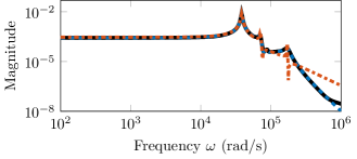
(a) Transfer functions.

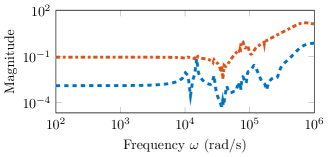
(b) Pointwise relative errors.

Figure 1: Results for the butterfly gyroscope data.

4.1 Butterfly gyroscope example

First, we present the results for the butterfly gyroscope model as shown in Figure 1. For the given data, we have used the two proposed approaches to learn structure-preserving models of order $r=8$. While SOVF2 converges up to numerical accuracy, this is not the case for SOVF1. However, the denominator in SOVF1 converges reasonably close to the value one. Consequently, we have simply considered the mechanical system associated with the rational function in the numerator of Eq. 13 and ignored the denominator entry altogether.

As it can be easily observed in Figure 1(a), SOVF1 accurately approximates the given data over the full frequency range. A minor exception is given by the right limit of the frequency interval, where the transfer function of SOVF1 slightly deviates from the data. On the other hand, SOVF2 lacks this good approximation behavior as it is illustrated in Figure 1(b). The accuracy of this approach is at least two orders of magnitude worse than that of SOVF1. Still, SOVF2 yields a reasonable approximation for the low frequency range. We have observed that SOVF2 typically introduces poles close to the imaginary axis, and has better approximation quality in the large magnitude range.

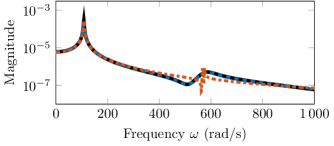
(a) Transfer functions.

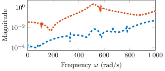
(b) Pointwise relative errors.

Figure 2: Results for the artificial fishtail data.

4.2 Artificial fishtail example

We now present results for the artificial fishtail example, as shown in Figure 2. We have used both approaches and constructed structure-preserving learned models of order $r=10$. As in the first example presented in Section 4.1, SOVF1 provides a high-fidelity approximation over the full frequency interval and outperforms SOVF2. As shown in Figure 2(b), the SOVF2 approximation has a large mismatch around $580$ rad/s, where the relative approximation error is the highest. Like in the previous example, SOVF2 to provides an accurate approximation of the main dominant peak, i.e., the one located around $100$ rad/s. Further details on the numerical results and convergence of the applied methods can be found in the accompanying code package.

5 Conclusions

We have proposed two new approaches for data-driven modeling of modally damped mechanical systems by developing structure-preserving vector fitting formulations. We have revised the barycentric formula to represent structured transfer functions, and have shown that the structure of the original model is automatically preserved in the reduced one. The two approaches have been applied to two benchmark models and the preliminary results are promising. The method corresponding to the partially structured transfer function formulation has been proven especially accurate and reliable in both test cases. A more thorough investigation is needed to explain the accuracy miss-matches encountered in the SOVF2 formulation. Extending the analysis and numerical algorithms to MIMO problems and employing the proposed structured barycentric forms to develop a AAA-like framework are natural next steps.

References

- [1] A. C. Antoulas and B. D. O. Anderson. On the scalar rational interpolation problem. IMA J. Math. Control Inf., 3(2–3):61–8, 1986. doi:10.1093/imamci/3.2-3.61.
- [2] C. Beattie and P. Benner. -optimality conditions for structured dynamical systems. Preprint MPIMD/14-18, Max Planck Institute for Dynamics of Complex Technical Systems Magdeburg, 2014.
- [3] P. Benner, P. Goyal, and I. Pontes Duff. Data-driven identification of Rayleigh-damped second-order systems. e-print 1910.00838, arXiv, 2020. math.OC, accepted for plubication in Realization and Model Reduction of Dynamical Systems. URL: http://arxiv.org/abs/1910.00838.
- [4] J.-P. Berrut and L. N. Trefethen. Barycentric Lagrange interpolation. SIAM Rev., 46(3):501–517, 2004. doi:10.1137/S0036144502417715.
- [5] Z. Drmač, S. Gugercin, and C. Beattie. Quadrature-based vector fitting for discretized approximation. SIAM J. Sci. Comput., 37(2):A625–A652, 2015. doi:10.1137/140961511.
- [6] Z. Drmač, S. Gugercin, and C. Beattie. Vector fitting for matrix-valued rational approximation. SIAM J. Sci. Comput., 37(5):A2346–A2379, 2015. doi:10.1137/15M1010774.
- [7] S. Grivet-Talocia and B. Gustavsen. Passive Macromodeling: Theory and Applications. Wiley Series in Microwave and Optical Engineering. John Wiley & Sons, Hoboken, NJ, 2015. doi:10.1002/9781119140931.
- [8] B. Gustavsen and A. Semlyen. Rational approximation of frequency domain responses by vector fitting. IEEE Trans. Power Del., 14(3):1052–1061, 1999. doi:10.1109/61.772353.
- [9] A. J. Mayo and A. C. Antoulas. A framework for the solution of the generalized realization problem. Linear Algebra Appl., 425(2–3):634–662, 2007. Special Issue in honor of P. A. Fuhrmann, Edited by A. C. Antoulas, U. Helmke, J. Rosenthal, V. Vinnikov, and E. Zerz. doi:10.1016/j.laa.2007.03.008.
- [10] Y. Nakatsukasa, O. Sète, and L. N. Trefethen. The AAA algorithm for rational approximation. SIAM J. Sci. Comput., 40(3):A1494–A1522, 2018. doi:10.1137/16M1106122.
- [11] Oberwolfach Benchmark Collection. Butterfly gyroscope. hosted at MORwiki – Model Order Reduction Wiki, 2004. URL: http://modelreduction.org/index.php/Butterfly_Gyroscope.
- [12] A. C. Rodriguez. Approximation of Parametric Dynamical Systems. PhD thesis, Virginia Polytechnic Institute and State University, Blacksburg, Virginia, USA, 2020. URL: http://hdl.handle.net/10919/99895.
- [13] J. Saak, D. Siebelts, and S. W. R. Werner. A comparison of second-order model order reduction methods for an artificial fishtail. at-Automatisierungstechnik, 67(8):648–667, 2019. doi:10.1515/auto-2019-0027.
- [14] C. Sanathanan and J. Koerner. Transfer function synthesis as a ratio of two complex polynomials. IEEE Trans. Autom. Control, 8(1):56–58, 1963. doi:10.1109/TAC.1963.1105517.
- [15] P. Schulze, B. Unger, C. Beattie, and S. Gugercin. Data-driven structured realization. Linear Algebra Appl., 537:250–286, 2018. doi:10.1016/j.laa.2017.09.030.
- [16] D. Siebelts, A. Kater, T. Meurer, and J. Andrej. Matrices for an artificial fishtail. hosted at MORwiki – Model Order Reduction Wiki, 2019. doi:10.5281/zenodo.2558728.
- [17] S. W. R. Werner. Structure-Preserving Model Reduction for Mechanical Systems. Dissertation, Department of Mathematics, Otto von Guericke University, Magdeburg, Germany, 2021. doi:10.25673/38617.