Nonlinear evolution of internal gravity waves in the Earth’s ionosphere: Analytical and numerical approach

Abstract

The nonlinear propagation of internal gravity waves in the weakly ionized, incompressible Earth’s ionosphere is studied using the fluid theory approach. Previous theory in the literature is advanced by the effects of the terrestrial inhomogeneous magnetic field embedded in weakly ionized ionospheric layers ranging in altitude from about $50$ to $500$ km. It is shown that the ionospheric conducting fluids can support the formation of solitary dipolar vortices (or modons). Both analytical and numerical solutions of the latter are obtained and analyzed. It is found that in absence of the Pedersen conductivity, different vortex structures with different space localization can be formed which can move with the supersonic velocity without any energy loss. However, its presence can cause the amplitude of the solitary vortices to decay with time and the vortex structure can completely disappear owing to the energy loss. Such energy loss can be delayed, i.e., the vortex structure can prevail for relatively a longer time if the nonlinear effects associated with either the stream function or the density variation become significantly higher than the dissipation due to the Pedersen conductivity. The main characteristic dynamic parameters are also defined which are in good correlation with the existing experimental data.

I Introduction

The internal gravity waves (GWs) are typically the low-frequency branch of acoustic gravity waves. Such waves are stimulated by the buoyancy forces arising from the vertical displacement of atmospheric particles in the gravitational field and are principally connected with the inhomogeneous distribution of medium density along the vertical direction (density stratification). Typical frequency of these internal GWs varies in the interval $10^{-4}$ s${}^{-1}<\omega<1.7\times\times 10^{-2}$ s^-1 and the typical wavelength is $\sim 10$ km. It should be noted that the internal GWs can propagate only in a stably stratified medium (in which the density of the medium increases vertically down) when the square of the Brunt-Väisälä frequency is positive, i.e., $\omega_{g}^{2}>0$. The transfer of wave energy to charged particles in the regions starting from the Earth’s lithosphere to the atmosphere and ionosphere is a fundamental problem of geophysics and applied research. The internal GWs play an important role in such s process. For example, internal GWs, propagating in the upward direction from the Earth’s surface to the upper atmosphere and ionosphere, are able to carry a large amount of energy and momentum. These waves are crucial in the atmospheric convection, generation of atmospheric turbulence and may affect global circulation. Theoretical and experimental studies over the last many years have shown that the source of acoustic GWs in the ionosphere can be earthquakes, volcanic eruptions, tornadoes, thunderstorms, solar eclipses, terminators, jet flows, polar and equatorial electrojets, meteors, strong explosions, and powerful rocket launches (see e.g., (Kato, 1980; Röttger, 1981; Fovell et al., 1992; Igarashi et al., 1994; Grigorev, 1999; Kanamori, 2004)).

The Earth’s and solar atmosphere provide a favorable environment for the generation and propagation of internal GWs. The internal GWs and related nonlinear structures are widely observed in the upper and lower layers of the atmosphere as well as in the lower ionosphere. In this context, a comprehensive review of GW dynamics and its effects in the Earth’s middle atmosphere has been given by Fritts and Alexander (Fritts and Alexander, 2003). Furthermore, the important roles of GWs in the vertical coupling of lower and upper atmospheres have been discussed in recent reviews (Yiǧit and Medvedev, 2015; Yiǧit et al., 2016). The most obvious gravity wave sources and experimental observations are widely discussed in this review (see for relevant details, e.g., (Swenson and Espy, 1995; Picard et al., 1998; Mitchell and Howells, 1998)). The atmospheric parameters and the onset of instability depend on season and altitude. Observations of the mesopause region ($80-105$ km) show that the probabilities of convective and the dynamic instability range from $1$ to $2$ and from $3$ to $10$ per cent respectively (Sherman and She, 2006; Zhao et al., 2003). Klausner et al. (Klausner et al., 2009) presented an experimental observation of the seasonal variation of gravity waves and the oscillations of traveling ionospheric disturbances in the ionospheric $F2$ layer during solar activity observed in different levels of geomagnetic activities. Observations of gravity wave characteristics in the Earth’s atmosphere were reviewed by Lu et al. (Lu et al., 2009). The observational results of acoustic GWs at ionospheric heights during convective storms were presented by Šindelár̃ová et al. (Šindelářová et al., 2009). Incoherent scatter radar power profile observations connected with acoustic GW propagation in the ionospheric $F$-region were discussed by Livneh et al. (Livneh et al., 2007). High-resolution radiosonde data was processed by Li et al. (Li et al., 2009) to obtain the gravity wave variability in the lower stratosphere over the South Pole. Parameters of internal GWs in the mesosphere/lower thermosphere regions from meteor radar wind data were revealed and described by Oleynikov et al. (Oleynikov et al., 2005) where previous experimental observations were are also listed. Recently, Izvekova et al. (Izvekova et al., 2015) had shown the possibility of acoustic GW instability in non-adiabatic terrestrial atmosphere.

Recently, Chatterjee and Misra (Chatterjee and Misra, 2021) advanced the nonlinear theory of acoustic GWs in the neutral atmosphere with the effects of the Coriolis force. Roy et al. (Roy et al., 2019) presented the nonlinear dynamical behaviors of acoustic GWs in the neutral atmosphere and possibility of tendency to chaotic states is shown. Kaladze et al. (Kaladze et al., 2018, 2019) studied the properties and peculiarities of linear three-dimensional propagation of electromagnetic internal GWs in an ideally conducting incompressible medium embedded in a uniform magnetic field. It is shown that the ordinary internal gravity waves can couple with Alfv’en waves. The existence of nonlinear acoustic GWs in the form of two-dimensional small-scale vortices (i.e., roll-type structures) in the neutral atmosphere has been reported by Stenflo and Shukla (Stenflo and Shukla, 2009). Onishchenko et al. (Onishchenko et al., 2013) have shown that the presence of finite temperature gradient can substantially modify the condition for the existence of vortex-type structures. It was noted that the vortices of internal GWs with the spatial scale $L$ smaller than the reduced height $H$ can be originated only in a convective unstable atmosphere. The amplitude of internal GWs propagating upward in various regions of the Earth’s atmosphere and ionosphere can grow with height and become unstable due to the parametric instability associated with the resonant wave-wave interactions. Such parametric generation of large scale zonal structures by high-frequency finite-amplitude internal GWs has been investigated recently by Horton et al. (Horton et al., 2008) and Onishchenko et al. (Onishchenko and Pokhotelov, 2012). The effects of the wind shear on the roll structures of nonlinear internal GWs in the Earth’s dynamically unstable atmosphere with the finite vertical temperature gradients were investigated by Onishchenko et al. (Onishchenko et al., 2014).

Theoretical investigation of the influence of charged particles and the inhomogeneous terrestrial magnetic field on the possibility of the formation of solitary vortical structures in different layers of the Earth’s weakly ionized ionosphere was started by Kaladze et al. (Kaladze and Tsamalashvili, 1997). The propagation of electromagnetic inertio-gravity waves in the earth’s partially ionized ionosphere was undertaken by Kaladze et al. (Kaladze et al., 2007, 2011a). The propagation characteristics of acoustic GWs in weakly ionized ionospheric $D$-, $E$-, and $F$-layers were investigated by Kaladze et al. (Kaladze et al., 2008a). It was shown that the incorporation of the Earth’s rotation provides a substantial change in the propagation dynamics of low-frequency internal GWs, namely, the existence of the new cut-off frequency at $2\Omega_{0}$ (where $\Omega_{0}$ is the value of the angular velocity of the Earth’s rotation) is noted. In addition, the authors noted that in the $E$ and $F$ layers of the ionosphere these waves decay with the damping rate of the same order of magnitude as in the linear case. Furthermore, the propagation of electromagnetic internal GWs coupled to Alfvén waves in the Earth’s ionospheric $E$-layer was investigated by Kaladze et. al. (Kaladze et al., 2011b). Also, the nonlinear generation of low-frequency and large-scale zonal flow and relatively small-scale electromagnetic coupled internal gravity and Alfvén waves in the Earth’s stratified weakly ionized ionospheric $E$-layer was investigated by Kaladze et al. (Kaladze et al., 2012). The influence of the DC electric field on the heating and instability of internal GWs leading to the formation of solitary vortex structures was studied by Chmyrev and Sorokin (Chmyrev and Sorokin, 2010). The nonlinear acoustic GWs, generated by seismic activity, propagating in the stable stratified ionospheric $E$-layer were shown (Kaladze et al., 2008b) to cause intensification of atomic oxygen green line emission when their amplitudes become sufficiently large. On the other hand, the importance of GWs in the global circulation of the middle and upper atmospheres has been recognized through various observational and theoretical studies. Using a general circulation model (GCM), the global distribution and the characteristics of GWs in these environments have been examined by a number of authors (Miyoshi and Fujiwara, 2008; Sato et al., 1999) to investigate the evolution of GWs and their momentum fluxes. In this context, different physical effects have been included in GCM to find estimates that conform with observational results. For example, the GW drag was included in the GCM and numerical prediction model to simulate a realistic stratospheric weak wind layer through various parameterizations (Iwasaki et al., 1989). Furthermore, using a nonlinear GW scheme, the variability of GW effects on the zonal mean circulation has been studied with the middle and upper atmospheric models (Lilienthal et al., 2020). Miyoshi et al. (Miyoshi and Fujiwara, 2008) studied the characteristics of GWs in the mesosphere and thermosphere using a GCM that includes the global distributions of electrons and ions. However, they commented that the model may not be appropriate to predict the ionospheric fluctuations induced by the neutral atmospheric variation.

In this paper, our aim is to advance the work of Kaladze et al. (Kaladze et al., 2008a) in investigating the existence and the nonlinear evolution of different kinds of solitary vortices that can be formed in the propagation of internal GWs in different layers of the Earth’s ionosphere. Using the fluid theory approach, a set of nonlinear coupled equations for the stream function and the density perturbation of atmospheric fluids is derived which governs the evolution of nonlinear solitary vortices. Both analytical and numerical studies are performed to obtain and analyze different kinds of stationary propagating dipolar vortical solutions as well as their dynamical evolution with the effects of Pedersen conductivity and the system nonlinearities. The manuscript is organized as follows. In Sec. II, the physical and mathematical modelings of internal GWs are described. While Sec. III is devoted to study analytically the existence of different kinds of stationary dipolar solitary vortices, the dynamical evolution of such dipolar vortices is studied numerically in Sec. IV. Finally, Sec. V is left for discussion and concluding our results.

II Physical and mathematical modeling

We consider the nonlinear propagation of internal gravity waves in the Earth’s ionospheric layers ($100-500$ km heights) stratified by the gravitational field. We assume that the ionospheric layers are weakly ionized and they consist of electrons, positive ions, and a bulk of massive neutral particles (i.e., $n/N\ll 1$, where $n$ and $N$, respectively, denote the equilibrium number densities of electrons or ions and neutrals). So, the presence of charged particles make the ionosphere to be electrically conducting. Due to strong collisions between the ionized and neutral particles, the dynamics of such electrically conducting ionosphere significantly differ from that of neutral atmosphere. Further we assume that the ionospheric plasma is immersed in the geomagnetic field $\mathbf{B}_{0}$ and is under the influence of the Coriolis force due to the Earth’s rotation with the angular velocity $\mathbf{\Omega}_{0}=(0,0,\Omega_{0})$. It follows that the interaction of the induced ionospheric current ($\mathbf{j}$) with the geomagnetic field ($\mathbf{B}$), i.e., the influence of the Ampére force ($\mathbf{j}\times\mathbf{B}$-force) should also be taken into consideration.

It is to be noted that for ionospheric disturbances the effective magnetic Reynolds’ number is relatively small in the ionospheric $D$, $E$, and $F$ regions, i.e., $R_{\text{eff}}\approx\mu_{0}\sigma_{\text{eff}}VL\sim VL/\eta_{m}\ll 1$, where $\mu_{0}=4\pi\times 10^{-7}$ H/m is the permeability of free space, $\eta_{m}$ is the magnetic diffusivity or plasma resistivity, $\sigma_{\text{eff}}\sim\sigma_{P}+\sigma_{H}^{2}/\sigma_{P}$ is the effective conductivity ($\sim 1/\eta\mu_{0}$) of the ionosphere with $\sigma_{H}$ denoting the Hall conductivity; and $V$ and $L$ are, respectively, the characteristic dimensions of velocity and space. So, for the lower ionosphere, one can neglect the induced magnetic field $\mathbf{b}=R_{\text{eff}}\mathbf{B}$ and the vortex part of the self-generated electric field $E_{v}\sim R_{\text{eff}}VB$ which originates due to the fluctuating magnetic field $\mathbf{b}$. Thus, for wave-like perturbations in the ionosphere we can consider the magnetic field as specified by the external geomagnetic field only, i.e., $\mathbf{B}=\mathbf{b}+\mathbf{B}_{0}\approx\mathbf{B}_{0}$ and $E_{v}\approx 0$ such that $\nabla\cdot\mathbf{B}_{0}=0$ and $\nabla\times\mathbf{B}_{0}=\mathbf{0}$. In this non-inductive approximation, it is sufficient to consider only the current $\mathbf{j}$ originating in the medium (Kaladze et al., 2008a) and the action of the geomagnetic field $\mathbf{B}_{0}$ on the induction current $\mathbf{j}$ in ionospheric plasmas makes it necessary to take into consideration the Ampére force in the equations for ionospheric dynamics. The most important impact of this force is the appearance of the inductive (magnetic) damping (due to the Pedersen currents) in the Earth’s ionosphere, which is no less significant than viscous breaking, especially in the $F$ region.

In what follows, the dynamics of the electrically conducting ionospheric plasmas can be described by the following momentum equation.

$$\frac{\partial\mathbf{u}}{\partial t}+\mathbf{u}\cdot\nabla\mathbf{u}=-\frac{\nabla p}{\rho}+\frac{\mathbf{j}\times\mathbf{B}_{0}}{\rho}+\mathbf{g},$$ (1)

where $\mathbf{j}$ is the current density, $\mathbf{u}$ is the bulk (neutral) velocity; $p$ and $\rho$ are the pressure and mass density of the medium, and $\mathbf{g}=(0,0,-g)$ is the acceleration due to gravity. Equation (1) is supplemented by the continuity equation and the equation of state, given by,

$$\frac{\partial\rho}{\partial t}+\nabla\cdot(\rho\mathbf{u})=0,$$ (2)

$$\left(\frac{\partial}{\partial t}+\mathbf{u}\cdot\nabla\right)\left(p-c_{s}^{2}\rho\right)=0,$$ (3)

where $c_{s}$ is the sound speed. The background pressure $p_{0}$ and the mass density $\rho_{0}$ are stratified by the gravitational field. They can be assumed to vary as $\rho_{0}(z)=\rho_{0}(0)\exp(-z/H)$ and $p_{0}(z)=p_{0}(0)\exp(-z/H)$, where $H=c_{s}^{2}/\gamma g$ is the reduced scale length of the atmosphere with $\gamma$ denoting the adiabatic constant. Since the ionosphere can be considered as quasineutral with a high degree of accuracy, we can ignore the inner electrostatic field, i.e., $\mathbf{E}=-\nabla\phi=\mathbf{0}$, where $\phi$ is the electrostatic potential, as well as the vortex components of the self-generated electromagnetic field. Thus, in the conducting medium, the electric field strength is determined only by the dynamo field $\mathbf{E}_{d}=\mathbf{u}\times\mathbf{B}_{0}$ and the generalized Ohm’s law reduces to

$$\mathbf{j}=\sigma_{\perp}\mathbf{E}_{d\perp}+\frac{\sigma_{H}}{B_{0}}\mathbf{B}_{0}\times\mathbf{E}_{d},$$ (4)

where $\sigma_{\perp}\equiv\sigma_{p}$ and $\sigma_{H}$, respectively, denote the perpendicular (Pedersen) and Hall conductivities. The subscripts $\parallel$ and $\perp$ denote the components parallel and perpendicular to the external magnetic field.

Next, we introduce a local Cartesian coordinate system with the $x$-axis directed from west to east, the $y$-axis from south to north, and the $z$-axis along the local vertical direction. We are primarily interested in the dynamics at high latitudes in the Northern Hemisphere, assuming that the geomagnetic field is vertical and downward, i.e., $\mathbf{B}_{0}=-B_{0}\hat{z}$. We consider the high-latitudes of the Northern Hemisphere to find evident analytic solutions. Also, in this region, the tropospheric flow is known to be much less zonal and the topography barriers are much less significant in the north–south orientation than those in the Southern Hemisphere (Garcia et al., 2017). Furthermore, for the internal GWs we consider $\mathbf{B}_{0}$ to be uniform and ignore the influence of the Coriolis force (Kaladze et al., 2008a). Also, to exclude the high-frequency acoustic mode we make use of the incompressibility condition, given by,

$$\nabla\cdot\mathbf{u}=0.$$ (5)

Equations (1) to (5) constitute a full set of equations necessary for the description of vortex motions of low-frequency incompressible internal GWs. For simplicity, we consider the two-dimensional motion of internal GWs in the $xz$-plane by assuming $\partial/\partial y\sim 0$. The incompressibility condition (5) allows us to introduce the stream function $\psi$, given by,

$$u=-\frac{\partial\psi}{\partial z},~{}~{}w=\frac{\partial\psi}{\partial x}$$ (6)

and the $y$-component of the vorticity vector $\nabla\times\mathbf{u}$ with $\mathbf{u}=(u,0,w)$ as

$$\zeta=\frac{\partial u}{\partial z}-\frac{\partial w}{\partial x}=-\left(\frac{\partial^{2}}{\partial x^{2}}+\frac{\partial^{2}}{\partial z^{2}}\right)\psi\equiv-\nabla^{2}\psi.$$ (7)

Following the work of Kaladze et al. (Kaladze et al., 2008a), we obtain the following system of equations which describe the nonlinear evolution of low-frequency internal GWs in the weakly ionized stable stratified Earth’s ionosphere.

$$\begin{split}\frac{\partial}{\partial t}\left(\nabla^{2}\psi-\frac{\psi}{4H^{2}}\right)&+J(\psi,\nabla^{2}\psi)=-\frac{\partial\chi}{\partial x}\\ &-\frac{\sigma_{p}B_{0}^{2}}{\rho_{0}}\left(\frac{\partial^{2}\psi}{\partial z^{2}}-\frac{\psi}{4H^{2}}\right),\end{split}$$ (8)

$$\frac{\partial\chi}{\partial t}+J(\psi,\chi)=\omega_{g}^{2}\frac{\partial\psi}{\partial x},$$ (9)

where $\omega_{g}=\sqrt{g/H}$ is the Brunt-Väisälä frequency for the incompressible fluid, the nonlinear term $J$ is the Jacobian, given by,

$$J(a,b)=\frac{\partial a}{\partial x}\frac{\partial b}{\partial z}-\frac{\partial a}{\partial z}\frac{\partial b}{\partial x},$$ (10)

and $\chi=g\rho/{\rho_{0}(0)}$ with $\rho$ denoting the perturbed mass density. Also, $\eta_{0}=\sigma_{p}B_{0}^{2}/\rho_{0}$ is the Pedersen parameter which produces the magnetic damping of internal GWs. From Eqs. (8) and (9) it is straightforward to obtain the following energy conservation equation.

$$\frac{\partial{\cal E}}{\partial t}+\eta_{0}\int\int\left[\left(\frac{\partial\psi}{\partial z}\right)^{2}+\frac{1}{4}\frac{\psi^{2}}{H^{2}}\right]dxdz=0,$$ (11)

where $\eta_{0}>0$ and ${\cal E}$ is the energy of the solitary vortex of internal GWs, given by,

$${\cal E}=\int\int\left[\frac{1}{2}\left(\nabla\psi\right)^{2}+\frac{1}{8}\frac{\psi^{2}}{H^{2}}+\frac{1}{2}\frac{\chi^{2}}{\omega_{g}^{2}}\right]dxdz.$$ (12)

Since the second term in Eq. (11) is positive definite, it follows from the $H$-theorem, stated as, If a distribution function of a particle $f(\mathbf{r},\mathbf{v},t)$ satisfies the Boltzmann transport equation, then the system evolves in such a manner that $dH/dt\leq 0$, and if $dH/dt=0$, then the system is in the equilibrium state, where $H$ is the functional, given by,

$$H(t)=\int f(\mathbf{r},\mathbf{v},t)\ln f(\mathbf{r},\mathbf{v},t)d^{3}rd^{3}v,$$ (13)

that $\partial{\cal E}/\partial t\leq 0$. Thus, the wave energy decays with time by the effects of the Pedersen parameter $\eta_{0}$ and so a steady-state solution with finite wave energy does not exist. Now, as per the estimations provided by Kaladze et al. (Kaladze et al., 2021), we have in the ionospheric $E$-layer the density ratio $n/N\sim 10^{-8}-10^{-6}$, the ion-neutral collision $\nu_{in}\lesssim 10^{3}~{}\mathrm{s}^{-1}$ so that the parameter $\eta_{0}\equiv\sigma_{p}B_{0}^{2}/\rho_{0}\sim\nu_{in}(n/N)$ varies in the interval $(10^{-8}-10^{-5})$ s^-1, while in the $F$-layer we have $n/N\sim 10^{-5}-10^{-3}$, $\nu_{in}\lesssim 10~{}\mathrm{s}^{-1}$ for which $\eta_{0}$ varies in $(10^{-6}-10^{-4})$ s^-1. Taking into account this estimation, we look for the linear solution of the system of Eqs. (8) and (9). To this end, we assume the perturbations to vary as plane waves $~{}\exp(ik_{x}x+ik_{z}z-i\omega t)$ with frequency $\omega$ and wave number $k$, and $\omega=\omega_{0}+i\gamma_{0}$, where $|\gamma_{0}|\ll\omega_{0}$. Thus, we obtain the following dispersion relation for the internal GWs (which is also valid for the ionospheric neutral $D$-layer). (Kaladze et al., 2008a)

$$\omega_{0}^{2}=\frac{k_{x}^{2}\omega_{g}^{2}}{k_{x}^{2}+k_{z}^{2}+1/4H^{2}},$$ (14)

and the wave damping rate (valid for $E$ and $F$ layers) as

$$\gamma_{0}=-\frac{1}{2}\eta_{0}\frac{k_{z}^{2}+1/4H^{2}}{k_{x}^{2}+k_{z}^{2}+1/4H^{2}}.$$ (15)

III Evolution of internal gravity solitary vortex: Analytical approach

The nonlinear behaviors of the low-frequency internal gravity waves is greatly influenced by the presence of the advective derivative. The corresponding vector nonlinearity (the Jacobian) can thus produce various coherent localized vortex structures for a broad range of background configurations. The forms of such vortices are strongly dependent on the spatial profile of the unperturbed medium. In a quiescent neutral atmosphere with the exponentially varying density and pressure profiles, the standard (spatially exponentially localized) travelling dipolar vortices (also called the internal gravity modons) have been found in an unstable stratified neutral $(\sigma_{p}=0)$ atmosphere with the transverse dimensions either much smaller (Stenflo, 1987), or comparable with the density scale length in a stable stratified neutral atmosphere (Stenflo and Stepanyants, 1995). It has been shown that such localized vortex structures can evolve in the form of circular vortices in inner $(r<a)$ and outer $(r>a)$ regions with $a$ denoting the radius of the circle (Stenflo, 1987; Shukla and Shaikh, 1998). Furthermore, by a numerical simulation approach it has been established that the dipoles associated with anti-cyclones in GWs can become more circular than cyclonic vortex and spread over a wide region of space (Snyder et al., 2007).

From Eq. (14) we conclude that the phase velocity $V_{\text{ph}}=\omega/k_{x}$ is limited by the interval

$$-V_{\text{max}}\leq V_{\text{ph}}\leq V_{\text{max}},$$ (16)

where in the case of the incompressible atmosphere, $V_{\text{max}}\sim 2H\omega_{g}=2\sqrt{gH}=2c_{s}/\sqrt{\gamma}$. Thus, when a source moves along the $x$-direction with a velocity larger than $V_{\text{max}}$, there is no resonance with the internal GWs. This means that such waves will not be generated by the source and hence no energy loss (Kaladze et al., 2008a). In this situation, one can obtain a stationary solution for the localization of a pulse propagating horizontally with a velocity $|V|>V_{\text{max}}$. An estimation with the reduced atmospheric height, $H\sim 6$ km gives $H\omega_{g}\sim 250$ m/s, i.e., $V_{\text{max}}\sim 500$ m/s. It follows that the nonlinear solitary vortex structure so formed becomes supersonic and its amplitude does not decay due to the generation of linear waves in the region $|V|<V_{\text{max}}$.

III.1 Standard stationary propagating internal gravity dipole vortical solution with $\eta_{0}\sim 0$

We note that in contrast to the equations in (Stenflo, 1987) and (Stenflo and Stepanyants, 1995), the nonlinear system of Eqs. (8) and (9) are obtained under the incompressibility condition (5), allowing to exclude the high-frequency acoustic gravity mode. To find the regular at the center and exponentially vanishing at infinity undamped travelling wave solution for $\eta_{0}\sim 0$, we consider the formation of internal gravity vortices in a frame moving with the constant velocity $U$ along the $x$-axis and thus apply the transformations $\xi=x-Ut$ and $z=z$. Furthermore, we consider the following linear relation between the mass density and the stream function.

$$\chi=-\frac{\omega_{g}^{2}}{U}\psi.$$ (17)

Substituting the relation (17) into Eq. (8), introducing a circle with radius $r=a$, dividing the integral domain in the inner $(r<a)$ and the outer $(r>a)$ regions, and following references (Stenflo, 1987) and (Stenflo and Stepanyants, 1995), we obtain the following dipole type vortex solutions in the polar coordinates $\xi=r\sin\phi,~{}z=r\cos\phi$.

$$\begin{split}&\nabla^{2}\psi_{i}=-Ak^{2}J_{1}(kr)\cos\phi,~{}~{}(r<a),\\ \mathrm{i.e.,}~{}&\psi_{i}=\left[AJ_{1}(kr)-\frac{k^{2}+p^{2}}{k^{2}}Ur\right]\cos\phi,~{}~{}(r<a)\end{split}$$ (18)

$$\begin{split}&\nabla^{2}\psi_{o}=Bp^{2}K_{1}(pr)\cos\phi,~{}~{}(r>a),\\ &~{}\mathrm{i.e.,}~{}\psi_{o}=BK_{1}(pr)\cos\phi,~{}~{}(r>a)\end{split}$$ (19)

where

$$p^{2}=\frac{1}{4H^{2}}-\frac{\omega_{g}^{2}}{U^{2}}>0.$$ (20)

Also, $J_{n}$ and $K_{n}$, respectively, stand for the Bessel function of first kind of order $n$ and the McDonald function of order $n$. In order that the circle $r=a$ to be a streamline we must have for the constant coefficients

$$A=\frac{p^{2}Ua}{k^{2}J_{1}(ka)},~{}~{}B=-\frac{Ua}{K_{1}(pa)}.$$ (21)

Furthermore, the continuity of $\partial\psi/\partial r$ on the circle $r=a$ requires the following parameter matching condition.

$$\frac{J_{2}(ka)}{kaJ_{1}(ka)}=-\frac{K_{2}(pa)}{paK_{1}(pa)},$$ (22)

which connects the parameters $k$, $p$, and $a$. Without loss of generality, any two of these parameters, say $k$ and $p$ can be taken as independent ones. So, two other parameters $U$ and $a$ still remain undefined in the solution. Thus, a stationary propagating nonlinear vortical solution for internal GWs can be written as

$$\psi(r,\phi)=aUF(r)\cos\phi,$$ (23)

where

$$F(r)=\left\{\begin{array}[]{cc}\frac{p^{2}}{k^{2}}\frac{J_{1}(kr)}{J_{1}(ka)}-\frac{(p^{2}+k^{2})r}{ak^{2}},&(r<a)\\ -\frac{K_{1}(pr)}{K_{1}(pa)},&(r\geq a)\end{array}\right.$$ (24)

We note that the solution (23) is antisymmetric with respect to the coordinate $z$. Also, the vorticity of velocity $\nabla^{2}\psi$ is continuous at $r=a$. The vortex solutions thus obtained are called dipole vortices. In addition, according to the condition $p^{2}>0$ [Eq. (20)], the vortical structure can propagate in both the positive and negative directions along the $x$-axis with the supersonic velocity $U$, satisfying the condition $U^{2}>V_{\text{max}}^{2}$. Thus, the velocity of the vortical flow $U$ has the values outside the regime $|V_{\text{ph}}|<V_{\text{max}}$ which is the regime of the phase velocity of linear periodic waves discussed before. So, there is no resonance with linear waves, implying that the vortices propagate quicker than linear waves due to the nonlinear amplitude. This means that these waves will not be produced by the source with no energy loss.

A profile of the vortex solution of Eq. (23) is shown in Fig. 1: (a) in the inner region $r<a$ where the dipolar vortex is formed and (b) in the outer region $r\geq a$ where no such dipole appears. The typical size of the vortex $a$ can be estimated by using Eq. (20) as

$$a\sim p^{-1}=\frac{2H|U|}{\left(U^{2}-4H^{2}\omega_{g}^{2}\right)^{1/2}}\approx 2H.$$ (25)

It is worthwhile to mention that the linear dispersion relation for internal GWs [Eq. (14)] can be recovered from Eq. (20) by the formal substitution:

$$p^{2}\rightarrow-(k_{x}^{2}+k_{z}^{2}),~{}U\rightarrow\frac{\omega_{0}}{k_{x}}.$$ (26)

!

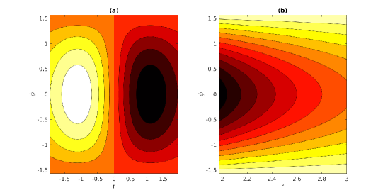
Figure 1: Contour plots of the stationary propagating vortical solution [Eq. (23)] are shown in the $r\phi$ plane for (a) $r<a$ and (b) $r\geq a$. The parameter values are $U/H\omega_{g}=3,~{}a/H=1.96,~{}p\sim a^{-1}$ and $k=2/H$.

III.2 Other stationary propagating internal gravity dipole vortical solution with $\eta_{0}\sim 0$

In this subsection, we find another vortex solution of Eqs. (9) and (8) by considering the following relation [instead of Eq. (17)].

$$\chi=-\omega_{g}H\nabla^{2}\psi.$$ (27)

In this case, Eqs. (8) and (9) reduce to

$$\frac{1}{4H^{2}}\frac{\partial\psi}{\partial t}+\omega_{g}H\frac{\partial}{\partial x}\nabla^{2}\psi+\frac{\omega_{g}}{H}\frac{\partial\psi}{\partial x}=0.$$ (28)

Transforming Eq. (28) into the moving frame of reference with coordinates $\xi=x-Ut$ and $z=z$, we obtain

$$\frac{\partial}{\partial\xi}\nabla^{2}\psi+\frac{1}{H^{2}}\left(1-\frac{1}{4}\frac{U}{H\omega_{g}}\right)\frac{\partial\psi}{\partial\xi}=0.$$ (29)

An integration of Eq. (29) with respect to $\xi$ yields

$$\nabla^{2}\psi+\frac{1}{H^{2}}\left(1-\frac{1}{4}\frac{U}{H\omega_{g}}\right)\psi=F(z),$$ (30)

where $F(z)$ is an arbitrary function of $z$. Next, looking for a solution of Eq. (30), which vanishes at infinity $[F(z)=0]$, we get

$$\psi=AJ_{1}(kr)\cos\phi,$$ (31)

where $A$ is a constant and

$$k^{2}=\frac{1}{H^{2}}\left(1-\frac{1}{4}\frac{U}{H\omega_{g}}\right)=\frac{1}{H^{2}}\left(1-\frac{1}{2}\frac{U}{V_{\text{max}}}\right)>0.$$ (32)

Now, as per Eq. (16), the positive velocity $U~{}(>0)$ should be larger than $V_{\text{max}}$ and it varies in the narrow interval $V_{\text{max}}<U<2V_{\text{max}}$. Thus, it follows that the solitary vortex with only the negative velocity can exist having the profile given by Eq. (31). It is also noted that the dipole vortex solution is regular at the centre $r=0$ and its amplitude $\propto 1/\sqrt{kr}$, i.e., vanishes at infinity. The vortex size can be estimated as $a\sim k^{-1}\sim H$.

In the case of large $U~{}(>0)$, Eq. (30) with $F(z)=0$ has the following solution.

$$\psi=BK_{1}(pr)\cos\phi,$$ (33)

where $B$ is a constant and

$$p^{2}=\frac{1}{H^{2}}\left(\frac{1}{4}\frac{U}{H\omega_{g}}-1\right)>0,$$ (34)

the positive velocity $U~{}(>4H\omega_{g})=2V_{\text{max}}$, and the negative velocities are inhibited. We note that the solution (33) has the singularity at the center $r=0$, however, it is exponentially localized in space $[\propto\exp(-pr)]$. Typical profiles of the vortex solutions of Eqs. (31) and (33) are shown in Fig. 2. The vortex size can be estimated as $a\sim p^{-1}\sim H$.

!

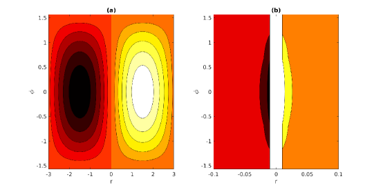
Figure 2: Contour plots of the stationary propagating vortical solutions [(a) Eq. (31) and (b) Eq. (33)] are shown in the $r\phi$ plane. The parameter values are $U/H\omega_{g}=-23$ for Eq. (31) and $U/H\omega_{g}=14.1$ for Eq. (33). The other parameters are $A=0.2$ and $B=2$.

III.3 An internal gravity dipole vortical solution with the effects of magnetic viscosity $(\eta_{0}\neq 0)$

On the basis of the multiple-scale analysis, we discuss the effects of the magnetic inhibition (The parameter $\eta_{0}$ may be called as the magnetic viscosity. The reason is that in the upper atmosphere with high latitudes, the geostrophic characters of fluid motions are almost lost, and they behave as in a viscous medium. Such viscosity, albeit similar to the magnetic viscosity, however, appears due to the inductive inhibition associated with the gyromotion of electrons and ions, electron-ion collisions, as well as collisions of neutrals with electrons and ions) on the vortical solution as described in Sec. III.2. To this end, we rewrite Eq. (28) with account of the magnetic inhibition term $\propto\eta_{0}=\sigma_{p}B_{0}^{2}/\rho_{0}$ as

$$\frac{1}{4H^{2}}\frac{\partial\psi}{\partial t}+\omega_{g}H\frac{\partial}{\partial x}\nabla^{2}\psi+\frac{\omega_{g}}{H}\frac{\partial\psi}{\partial x}-\eta_{0}\left(\frac{\partial^{2}}{\partial z^{2}}-\frac{1}{4H^{2}}\right)\psi=0.$$ (35)

Assuming that the effect of the magnetic inhibition on the wave damping is small, i.e., $\eta_{0}\sim o(\epsilon)$, we introduce a slow time scale $t_{1}=\eta_{0}t$ and represent $\psi$ as

$$\psi(t)=\psi^{(1)}(t,t_{1})+\eta_{0}\psi^{(2)}(t,t_{1})+{\cal O}(\eta_{0}^{2}),$$ (36)

which applies for longer times, i.e., $t\sim{\cal O}(1/\eta_{0})$. Substituting the perturbation expansion (36) into Eq. (35), we obtain the following first and second order equations.

$$\frac{1}{4H^{2}}\frac{\partial\psi^{(1)}}{\partial t}+\omega_{g}H\frac{\partial}{\partial x}\nabla^{2}\psi^{(1)}+\frac{\omega_{g}}{H}\frac{\partial\psi^{(1)}}{\partial x}=0,$$ (37)

$$\begin{split}\frac{1}{4H^{2}}\frac{\partial\psi^{(2)}}{\partial t}+\omega_{g}H\frac{\partial}{\partial x}\nabla^{2}\psi^{(2)}&+\frac{\omega_{g}}{H}\frac{\partial\psi^{(2)}}{\partial x}=-\frac{1}{4H^{2}}\frac{\partial\psi^{(1)}}{\partial t_{1}}\\ &-\frac{1}{4H^{2}}\psi^{(1)}+\frac{\partial^{2}\psi^{(1)}}{\partial z^{2}}.\end{split}$$ (38)

Equation (37) for $\psi^{(1)}(t,t_{1})$ describes the solutions (31) and (33) with the coefficients $A(t_{1})$ and $B(t_{1})$ respectively. The secular terms on the right-hand side of Eq. (38) (except the last term on the right-hand side, i.e., the source term) can be prevented by imposing the following solvability condition.

$$\frac{\partial\psi^{(1)}}{\partial t_{1}}+\psi^{(1)}=0.$$ (39)

A solution of Eq. (39) modulates the coefficients $A(t_{1})$ and $B(t_{1})$ as well as the profiles (31) and (33) as

$$\begin{split}&\psi=A_{0}\exp(-\eta_{0}t)J_{1}(kr)\cos\phi,\\ &\chi=B_{0}\exp(-\eta_{0}t)K_{1}(pr)\cos\phi,\end{split}$$ (40)

where $A_{0}$ and $B_{0}$, evaluated at $t=0$, are constants. Clearly, the amplitude of the solitary vortex decays as time goes on by the effects of the magnetic viscosity.

IV Evolution of internal gravity solitary vortex: Numerical approach

Before we numerically study the system of Eqs. (8) and (9) for the evolution of dipolar vortices of internal GWs, it is pertinent to make the system dimensionless. So, redefining the variables, namely

$$\begin{split}&(x,z)\rightarrow(x,z)/H,~{}t\rightarrow t\omega_{g},~{}\psi\rightarrow\psi/\psi_{0},~{}\chi\rightarrow\chi/\chi_{0},\\ &\alpha=\psi_{0}/\omega_{g}H^{2},~{}\beta=H\chi_{0}/\omega_{g}\psi_{0},~{}\eta=\sigma_{p}B_{0}^{2}/\rho_{0}\omega_{g},\end{split}$$ (41)

we obtain from Eqs. (8) and (9) the following reduced evolution equations.

$$\begin{split}\frac{\partial}{\partial t}\left(\nabla^{2}\psi-\frac{1}{4}\psi\right)&+\alpha\left(\frac{\partial\psi}{\partial x}\frac{\partial\nabla^{2}\psi}{\partial z}-\frac{\partial\psi}{\partial z}\frac{\partial\nabla^{2}\psi}{\partial x}\right)\\ &=-\beta\frac{\partial\chi}{\partial x}-\eta\left(\frac{\partial^{2}\psi}{\partial z^{2}}-\frac{1}{4}\psi\right),\end{split}$$ (42)

$$\frac{\partial\chi}{\partial t}+\alpha\left(\frac{\partial\psi}{\partial x}\frac{\partial\chi}{\partial z}-\frac{\partial\psi}{\partial z}\frac{\partial\chi}{\partial x}\right)=\frac{1}{\beta}\frac{\partial\psi}{\partial x}.$$ (43)

Here, we note that the dimensionless parameters $\alpha$, $\beta$ and $\eta$ are, respectively, associated with the Jacobian nonlinearities for the stream function and density variation; the length $(H)$ and the time $(\omega_{g}^{-1})$ scales; and the Pedersen conductivity. In order to investigate the global behaviors of solitary vortices we numerically solve Eqs. (42) and (43) by the standard 4-th order Runge-Kutta scheme with the time step $dt=10^{-4}$, the mesh size $dx=dz\sim 0.1$ and the initial condition in the form of a two-dimensional sinusoidal wave. The spatial derivatives were approximated by the centered second-order difference formulas. Furthermore, in order to study the qualitative behaviors of solitary vortices we have considered the parameter values that are relevant, e.g., in the ionospheric $F$-layer. Also, $\psi_{0}\sim\omega_{g}H^{2}$, $\chi_{0}\sim\omega_{g}^{2}/H$, so that $\alpha,~{}\beta\sim 1$, and $\eta\sim 10^{-2}-10^{-1}$ depending on the magnetic field strength. The results are displayed in Figs. 3 to 6. It is observed that the initial profile evolves and as time goes the nonlinearities (Jacobian) associated with the stream function and the density variation, and the vorticity function intervene to form a dipolar structure. However, the vortical structure tends to disappear when the Pedersen parameter $\eta$ exceeds a critical value. The decay of the wave amplitude becomes faster the larger is the values of $\eta$.

Figure 3 shows the profiles of the solitary vortex at different times with the parameters $\alpha=1.09$, $\beta=1.02$ and $\eta=0.18$. From Fig. 3 we find that when the effect of the Pedersen parameter is small, i.e., $\eta=0.18$, the decay rate of the wave amplitude is relatively slow for which the dipolar vortex structure can be seen for a longer time. However, as its value is increased from $\eta=0.18$ to $\eta=0.215$, Fig. 4 shows that the vortex structure tends to disappear with time and it completely disappears after time $t=80$ due to the energy loss by the magnetic viscosity. Keeping the values of $\eta$ and $\beta$ fixed at $0.215$ and $1.02$, as the value of $\alpha$ is increased from $\alpha=1.09$ to $\alpha=1.59$, the nonlinearity intervenes to compensate the energy loss. As a result, the vortex structure prevails even for a longer time [See Fig. 5]. The similar phenomena can happen with an increasing value of $\beta$, say from $\beta=1.02$ to $\beta=1.52$ keeping others fixed at $\alpha=1.09$ and $\eta=0.215$ [See Fig. 6]. Physically, when the parameter $\beta$ is increased, from the energy expression [Eq. (12)] it follows that the nonlinearity associated with the density perturbation also increases, which in turn increases the wave energy ${\cal E}$ and contributes to the energy loss for a limited period of time. As a result, the wave damping becomes slower and the dipolar structure prevails for relatively a longer time.

!

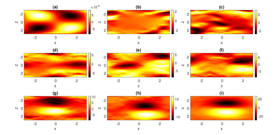
Figure 3: The evolution of solitary dipolar vortex [Numerical simulations of Eqs. (42) and (43)] is shown at different times from (a) $t=0$ to (i) $t=80$ with an interval of $t=10$. The parameter values are $\alpha=1.09$, $\beta=1.02$ and $\eta=0.18$.

!

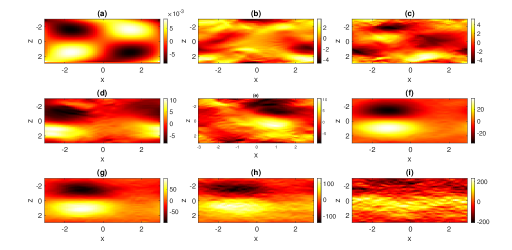
Figure 4: The same as in Fig. 3 but with a different value of $\eta=0.215$. The other parameter values are $\alpha=1.09$ and $\beta=1.02$.

!

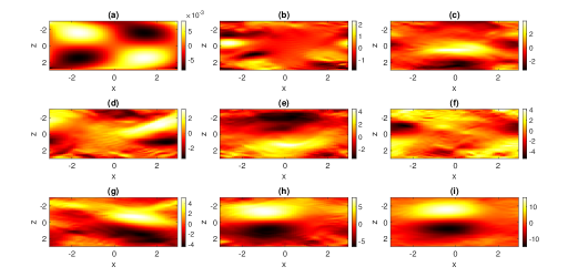
Figure 5: The same as in Fig. 4 but with a different value of $\alpha=1.59$. The other parameter values are $\beta=1.02$ and $\eta=0.215$.

!

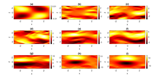
Figure 6: The same as in Fig. 5 but with a different value of $\beta=1.52$. The other parameter values are $\alpha=1.09$ and $\eta=0.215$.

V Discussion and Conclusion

Starting from a set of nonlinear coupled equations (Kaladze et al., 2008a) for the stream function and the density variations of atmospheric fluids, we have studied the nonlinear evolution of internal GWs in the Earth’s weakly ionized stratified conductive ionosphere. The model equations are based on some physical assumptions. According to observations, the internal GWs exist in a large range of heights extending from the mesosphere to the ionosphere ($50-500$ km). At such heights, the Earth’s ionosphere (overlapping into the mesosphere and thermosphere) is conductive due to the presence of charged particles and neutral atoms. In the model, we have considered the current arising in the gas but neglected the vortex parts of the self-generated electromagnetic fields using the so-called non-inductive approximation. Thus, only the dynamo electric field comes into the picture. Specifically, we have focused on the nonlinear dynamics of internal GWs at high latitudes in the northern hemisphere assuming that the geomagnetic field is vertical and directed downward. The ionospheric gas is highly stratified and accordingly, we have considered an isothermal incompressible atmosphere for the adiabatic propagation of internal GWs.

In the small amplitude limit (linear approximation), we have obtained the dispersion relation for internal GWs propagating along the $x$-axis with a frequency lower than than the Brunt-Väisälä frequency $\omega_{g}$. It is seen that the eigen frequency varies in the regime $10^{-4}$ s${}^{-1}<\omega_{0}<1.7\times 10^{-2}$ s^-1 and the typical wavelength is $\lambda\sim H\sim 10$ km. Also, the phase velocity and the group velocity are of the same order, i.e., $v_{p}\sim v_{g}\sim V_{\text{max}}\sim 6\times 10^{2}$ m/s. Such an estimate agrees with some existing observations made by Šindelár̃ová et al. (Šindelářová et al., 2009). Furthermore, it is shown that the acting electromagnetic force is defined by the Pedersen conductivity $(\sigma_{p})$ leading to the so-called magnetic inhibition (damping) of internal GWs with the decrement rate proportional to the Padersen parameter $\eta\equiv\sigma_{p}B_{0}^{2}/\rho_{0}\omega_{g}$. This damping rate increases with the magnetic field strength and for parameter values relevant for the ionospheric $F$-layer. Its value can be estimated as $|\gamma_{0}|\sim\eta_{0}\sim 10^{-4}$ s^-1. Due to the small damping rate compared to the eigen frequency $\omega_{0}\lesssim\omega_{g}\sim 10^{-2}$ s^-1, the linear internal GWs can grow to a nonlinear stage and form vortical structures whose evolution is described by a coupled set of nonlinear equations (42) and (43). The coupled set of equations is solved analytically to obtain various vortical solutions with different space localization. Furthermore, the equations are also solved numerically to ascertain the occurrence of internal gravity dipolar vortices. The internal GWs and related nonlinear structures are widely observed in the upper and lower layers of the atmosphere as well as in the lower ionosphere, (see for details, e.g., (Fritts and Alexander, 2003; Swenson and Espy, 1995; Picard et al., 1998; Lu et al., 2009; Mitchell and Howells, 1998; Šindelářová et al., 2009). Also, such solitary dipolar vortices were discovered in Freja satellite observations of space plasmas (Louarn et al., 1994; Wu et al., 1996). In this context, the differences of the numerical approach implemented here with some other models, e.g., (Gavrilov et al., 2020; Hickey et al., 2015) can be noted. Gavrilov et al. (Gavrilov et al., 2020) used the high-resolution model “AtmoSym” for three-dimensional simulation of acoustic GWs with background vertical profiles of temperature, molecular weight, density, molecular viscosity and heat conduction corresponding to various solar activity (SA) levels. Their numerical modeling revealed large amplitude temperature perturbations at heights above $150$ km with high SA. On the other hand, a full wave model was proposed for a binary gas by Hickey et al. (Hickey et al., 2015) to study the effects of thermal conductivity and viscosity on the propagation of GWs in the thermosphere.

The following new results are obtained.

• For a particular choice of the mass density $\chi$ as a function of the stream function $\psi$, i.e., $\chi=-(\omega_{g}^{2}/U)\psi$, we have obtained a new kind of stationary propagating $(\eta_{0}=0)$ standard dipole vortical solution (23). The vortical structures can propagate in both the positive (to the East) and negative (to the West) directions of the $x$-axis with the supersonic velocity $U$, satisfying $U^{2}>V^{2}_{\text{max}}$ and thereby preventing the generation of linear waves by the moving structure (since the phase velocity is limited by $V_{\text{ph}}\leq V_{\text{max}}$). Typical size of the vortex is $a\sim 2H\sim 15$ km. Furthermore, the vortex structures are exponentially localized in space and regular at the center.

• In an another case with $\chi=-\omega_{g}H\nabla^{2}\psi$, we have obtained another class of stationary propagating $(\eta_{0}=0)$ vortical solutions [Eqs. (31) and (33)]. The positive velocity $U$ of the structure [Eq. (31)] is found to be larger than $V_{\text{max}}$ and it may vary in the narrow regime $V_{\text{max}}<U<2V_{\text{max}}$. Thus, only the structures with negative velocities can mainly appear. It is found that the vortex solution is regular at the center $r=0$ and it vanishes at infinity $(\propto 1/\sqrt{kr})$. The vortex size can be estimated as $a\sim k^{-1}\sim H\sim 10$ km. On the other hand, the vortical structure corresponding to the the solution (33) can propagate with the positive velocity $U>4H\omega_{g}\sim 2V\text{max}$, while the negative velocities (motions to the West) are inhibited. This dipolar vortex solution has the singularity at the center $r=0$, but is exponentially localized in space $[\propto\exp(-pr)]$. The vortex size can be estimated as $a\sim p^{-1}\sim H\sim 10$ km.

• Using the multiple-scale method approximate vortical solutions (40) of Eqs. (8) and (9) are also obtained with $\chi=-\omega_{g}H\nabla^{2}\psi$ by the influence of weak magnetic inhibition (viscosity). It is shown that the amplitude of the solitary vortex profile decays exponentially with time, i.e., the internal GWs undergo weak damping due to a small effect of the Pedersen parameter. Such vortical structures exist during the time $t\sim 1/\eta_{0}$ which constitutes $t\sim 30-3\times 10^{6}$ h for the $E$-layer and $30-300$ h for the $F$-layer.

• Numerical simulations of dimensionless Eqs. (42) and (43) reveal that the solitary dipolar vortex profile can appear and propagate for a longer time until the dissipation due to the Pedersen conductivity $(\sim\eta\equiv\eta_{0}/\omega_{g})$ is negligible. When the effect of $\eta$ is relatively strong, the vortex structure tends to disappear as time goes on and it completely disappears after a certain time due to the energy loss by the magnetic viscosity. However, the energy loss can reduced or the vortex structure can prevail for relatively a longer time if the nonlinear effects associated with either the stream function or the density variation or both become significantly higher than that due to the dissipation.

To conclude, the theoretical results should be useful for understanding the characteristics of low frequency internal gravity waves and the formation of solitary dipolar vortex in the Earth’s ionosphere. Such vortical structures carry trapped particles and contribute to essentially transport of plasma particles in atmospheric conducting fluids. Thus, they can play crucial roles for understanding coupling of the ionosphere with lower-lying regions.

References

- Kato (1980) S. Kato, Dynamics of the Upper Atmosphere (Springer, Netherlands, 1980).
- Röttger (1981) J. Röttger, Journal of Atmospheric and Solar-Terrestrial Physics 43, 453 (1981).
- Fovell et al. (1992) R. Fovell, D. Durran, and J. Holton, Journal of the Atmospheric Sciences 49, 1427 (1992).
- Igarashi et al. (1994) K. Igarashi, S. Kainuma, I. Nishimuta, S. Okamoto, H. Kuroiwa, T. Tanaka, and T. Ogawa, Journal of Atmospheric and Solar-Terrestrial Physics 56, 1227 (1994).
- Grigorev (1999) G. I. Grigorev, Radiophysics and Quantum Electronics 42, 1 (1999).
- Kanamori (2004) H. Kanamori, Fluid Dynamics Research 34, 1 (2004).
- Fritts and Alexander (2003) D. Fritts and M. Alexander, Reviews of Geophysics 41, 1003 (2003).
- Yiǧit and Medvedev (2015) E. Yiǧit and A. S. Medvedev, Advances in Space Research 55, 983 (2015).
- Yiǧit et al. (2016) E. Yiǧit, P. Koucká Knížová, K. Georgieva, and W. Ward, Journal of Atmospheric and Solar-Terrestrial Physics 141, 1 (2016), sI:Vertical Coupling.
- Swenson and Espy (1995) G. Swenson and P. Espy, Geophysical Research Letters 22, 2845 (1995).
- Picard et al. (1998) R. H. Picard, R. O’Neil, H. Gardiner, J. Gibson, J. Winick, W. Gallery, A. T. Stair, P. Wintersteiner, E. R. Hegblom, and E. Richards, Geophysical Research Letters 25, 2809 (1998).
- Mitchell and Howells (1998) N. Mitchell and V. Howells, Annales Geophysicae 16, 1367 (1998).
- Sherman and She (2006) J. Sherman and C. She, Journal of Atmospheric and Solar-Terrestrial Physics 68, 1061 (2006).
- Zhao et al. (2003) Y. Zhao, A. Liu, and C. Gardner, Journal of Atmospheric and Solar-Terrestrial Physics 65, 219 (2003).
- Klausner et al. (2009) V. Klausner, P. Fagundes, Y. Sahai, C. Wrasse, V. G. Pillat, and F. Becker-Guedes, Journal of Geophysical Research 114 (2009), 10.1029/2008JA013448.
- Lu et al. (2009) X. Lu, A. Liu, G. Swenson, T. Li, T. Leblanc, and I. McDermid, Journal of Geophysical Research 114 (2009), https://doi.org/10.1029/2008JD010112.
- Šindelářová et al. (2009) T. Šindelářová, D. Burešová, and J. Chum, Studia Geophysica et Geodaetica 53, 403 (2009).
- Livneh et al. (2007) D. J. Livneh, I. Seker, F. Djuth, and J. Mathews, Journal of Geophysical Research 112 (2007), https://doi.org/10.1029/2006JA012225.
- Li et al. (2009) Z. Li, W. Robinson, and A. Liu, Journal of Geophysical Research 114 (2009), 10.1029/2008JD011478.
- Oleynikov et al. (2005) A. Oleynikov, C. Jacobi, and D. M. Sosnovchik, Annales Geophysicae 23, 3431 (2005).
- Izvekova et al. (2015) Y. Izvekova, S. Popel, and B. B. Chen, Journal of Atmospheric and Solar-Terrestrial Physics 134, 41 (2015).
- Chatterjee and Misra (2021) D. Chatterjee and A. Misra, Journal of Atmospheric and Solar-Terrestrial Physics 222, 105722 (2021).
- Roy et al. (2019) A. Roy, S. Roy, and A. P. Misra, Journal of Atmospheric and Solar-Terrestrial Physics 186, 78 (2019).
- Kaladze et al. (2018) T. Kaladze, L. V. Tsamalashvili, and D. T. Kaladze, 2018 XXIIIrd International Seminar/Workshop on Direct and Inverse Problems of Electromagnetic and Acoustic Wave Theory (DIPED) , 35 (2018).
- Kaladze et al. (2019) T. Kaladze, L. Tsamalashvili, and D. Kaladze, Journal of Atmospheric and Solar-Terrestrial Physics 182, 177 (2019).
- Stenflo and Shukla (2009) L. Stenflo and P. Shukla, Journal of Plasma Physics 75, 841 (2009).
- Onishchenko et al. (2013) O. Onishchenko, O. Pokhotelov, and V. Fedun, Annales Geophysicae 31, 459 (2013).
- Horton et al. (2008) W. Horton, T. Kaladze, J. V. Dam, and T. Garner, Journal of Geophysical Research 113, A08312 (2008).
- Onishchenko and Pokhotelov (2012) O. Onishchenko and O. Pokhotelov, Doklady Earth Sciences 445, 845 (2012).
- Onishchenko et al. (2014) O. Onishchenko, O. Pokhotelov, W. Horton, A. Smolyakov, T. Kaladze, and V. Fedun, Annales Geophysicae 32, 181 (2014).
- Kaladze and Tsamalashvili (1997) T. Kaladze and L. V. Tsamalashvili, Physics Letters A 232, 269 (1997).
- Kaladze et al. (2007) T. D. Kaladze, O. A. Pokhotelov, L. Stenflo, H. A. Shah, and G. V. Jandieri, Physica Scripta 76, 343 (2007).
- Kaladze et al. (2011a) T. Kaladze, L. Tsamalashvili, and L. Kahlon, Journal of Atmospheric and Solar-Terrestrial Physics 73, 741 (2011a).
- Kaladze et al. (2008a) T. Kaladze, O. Pokhotelov, H. Shah, M. Khan, and L. Stenflo, Journal of Atmospheric and Solar-Terrestrial Physics 70, 1607 (2008a).
- Kaladze et al. (2011b) T. Kaladze, L. Tsamalashvili, and D. Kaladze, Physics Letters A 376, 123 (2011b).
- Kaladze et al. (2012) T. Kaladze, L. Kahlon, L. Tsamalashvili, and D. Kaladze, Journal of Atmospheric and Solar-Terrestrial Physics 89, 110 (2012).
- Chmyrev and Sorokin (2010) V. Chmyrev and V. Sorokin, Journal of Atmospheric and Solar-Terrestrial Physics 72, 992 (2010).
- Kaladze et al. (2008b) T. Kaladze, W. Horton, T. Garner, J. V. Dam, and M. L. Mays, Journal of Geophysical Research 113, A12307 (2008b).
- Miyoshi and Fujiwara (2008) Y. Miyoshi and H. Fujiwara, Journal of Geophysical Research: Atmospheres 113 (2008), https://doi.org/10.1029/2007JD008874, https://agupubs.onlinelibrary.wiley.com/doi/pdf/10.1029/2007JD008874 .
- Sato et al. (1999) K. Sato, T. Kumakura, and M. Takahashi, Journal of the Atmospheric Sciences 56, 1005 (1999).
- Iwasaki et al. (1989) T. Iwasaki, S. Yamada, and K. Tada, Journal of the Meteorological Society of Japan. Ser. II 67, 11 (1989).
- Lilienthal et al. (2020) F. Lilienthal, E. Yiğit, N. Samtleben, and C. Jacobi, Frontiers in Astronomy and Space Sciences 7 (2020), 10.3389/fspas.2020.588956.
- Garcia et al. (2017) R. R. Garcia, A. K. Smith, D. E. Kinnison, Álvaro de la Cámara, and D. J. Murphy, Journal of the Atmospheric Sciences 74, 275 (2017).
- Kaladze et al. (2021) T. Kaladze, O. Özcan, A. Yesil, L. V. Tsamalashvili, D. T. Kaladze, M. Inç, S. Sagir, and K. Kurt, Zeitschrift für Angewandte Mathematik und Physik 72, 1 (2021).
- Stenflo (1987) L. Stenflo, Physics of Fluids 30, 3297 (1987).
- Stenflo and Stepanyants (1995) L. Stenflo and Y. A. Stepanyants, Annales Geophysicae 13, 973 (1995).
- Shukla and Shaikh (1998) P. K. Shukla and A. A. Shaikh, Physica Scripta T75, 247 (1998).
- Snyder et al. (2007) C. Snyder, D. J. Muraki, R. Plougonven, and F. Zhang, Journal of the Atmospheric Sciences 64, 4417 (2007).
- Louarn et al. (1994) P. Louarn, J. E. Wahlund, T. Chust, H. de Feraudy, A. Roux, B. Holback, P. O. Dovner, A. I. Eriksson, and G. Holmgren, Geophysical Research Letters 21, 1847 (1994), https://agupubs.onlinelibrary.wiley.com/doi/pdf/10.1029/94GL00882 .
- Wu et al. (1996) D. J. Wu, G. L. Huang, and D. Y. Wang, Phys. Rev. Lett. 77, 4346 (1996).
- Gavrilov et al. (2020) N. M. Gavrilov, S. P. Kshevetskii, and A. V. Koval, Journal of Atmospheric and Solar-Terrestrial Physics 208, 105381 (2020).
- Hickey et al. (2015) M. P. Hickey, R. L. Walterscheid, and G. Schubert, Journal of Geophysical Research: Space Physics 120, 3074 (2015), https://agupubs.onlinelibrary.wiley.com/doi/pdf/10.1002/2014JA020583 .