Graph Partner Neural Networks for Semi-Supervised Learning on Graphs

Abstract

Graph Convolutional Networks (GCNs) are powerful for processing graph-structured data and have achieved state-of-the-art performance in several tasks such as node classification, link prediction, and graph classification. However, it is inevitable for deep GCNs to suffer from an over-smoothing issue that the representations of nodes will tend to be indistinguishable after repeated graph convolution operations. To address this problem, we propose the Graph Partner Neural Network (GPNN) which incorporates a de-parameterized GCN and a parameter-sharing MLP. We provide empirical and theoretical evidence to demonstrate the effectiveness of the proposed MLP partner on tackling over-smoothing while benefiting from appropriate smoothness. To further tackle over-smoothing and regulate the learning process, we introduce a well-designed consistency contrastive loss and Kullback–Leibler (KL) divergence loss. Besides, we present a graph enhancement technique to improve the overall quality of edges in graphs. While most GCNs can work with shallow architecture only, GPNN can obtain better results through increasing model depth. Experiments on various node classification tasks have demonstrated the state-of-the-art performance of GPNN. Meanwhile, extensive ablation studies are conducted to investigate the contributions of each component in tackling over-smoothing and improving performance.

1 Introduction

Recently, Graph Neural Networks (GNNs) have become a hot topic in deep learning for the potentials in modeling non-Euclidean data. Early works  Zhu et al. (2003); Zhou et al. (2003); Belkin et al. (2006) adopt some form of explicit graph laplacian regularization, which restricts the flexibility and expressive power of GNNs. Later methods can be divided into two categories, namely the spectral-based methods and the spatial-based ones Wu et al. (2021). Graph Convolutional Network (GCN)  Kipf and Welling (2017) bridges the above two categories via a first-order Chebyshev approximation of the spectral graph convolutions, which is similar to perform message passing operations on neighbor nodes.

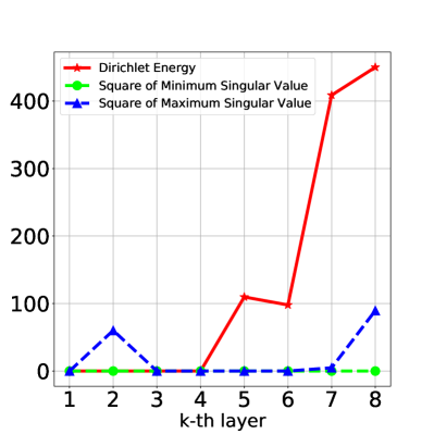
(a) Dirichlet energy of node embeddings, the squares of maximum and minimum singular values of weight matrix at the k-th layer of a 8-layer GCN on Cora dataset.

(b) visualization of node embeddings of the 4-th layer.

Figure 1: Impact of feature transformation on over-smoothing. The Dirichlet energy at the first 4 layers is almost zero, which reveals that the pairwise distances are almost zero and the node embeddings are indistinguishable . We argue that the extremely small singular values of weight matrices give rise to this phenomenon.

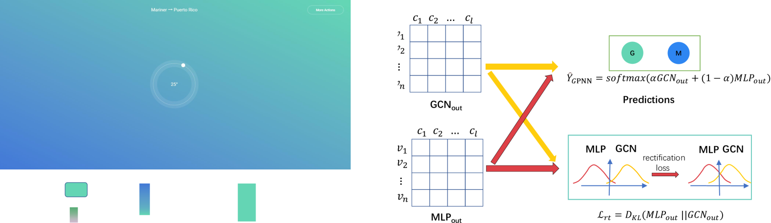
Figure 2: Overall architecture of the proposed model. We first perform graph enhancement to generate a new graph that incorporates the node attribute as supplemental information. The blue lines in the enhanced graph denote original edges in the graph, and the dotted lines represent newly added edges by graph enhancement. Then the input feature matrix, $\mathbf{X}$, is fed into the two branches of the model, respectively. The yellow lines represent the GCN branch which consists of a linear transformation along with an l-step feature propagation and another linear transformation. The Red lines represent the MLP branch including two 1-layer linear transformation. The two weight matrices of transformations are shared and trained jointly. Finally, the outputs of GCN and MLP are used to predict labels together and a rectification loss is calculated based on the KL divergence between them, which can be used to ensure consistency between the two branches. For clarify purposes, the contrastive loss is not depicted.

Deep neural networks usually achieve better performance compared with shallow ones, but it is not the case in graph neural networks  Velickovic et al. (2019). Most GNNs obtain better results with a shallow structure, for example, GCN and GAT  Velickovic et al. (2018) achieve their best performance at 2 layers. Repeated graph convolution operations can be approximated with a generalization of a Markov process, where the propagation matrix can be viewed as a generalized transition matrix. Notably, under certain conditions, a Markov process will exponentially converge to a steady state that is irrelevant to the initial state  Chung and Graham (1997). In the context of our task, multiple graph convolution operations make the representations of nodes tend to be the same, i.e., indistinguishable and lose expressiveness, which is called over-smoothing. To tackle the over-smoothing issue in deep architectures, many approaches have been presented. Inspired by Oono and Suzuki (2020), DropEdge  Rong et al. (2020) suggests that over-smoothing can be relieved by randomly removing a fraction of edges from the input graph at each epoch. JKNet  Xu et al. (2018) finds it useful to reuse distinguishable features of the shallow layers, thus feeds previous layers’ outputs into the last layer. Likewise, GCNII  Chen et al. (2020b) adopts the initial residual and identity mapping technique to retain initial information.

Although these methods have alleviated over-smoothing via randomizing the propagation or reusing information from previous layers, they ignore the impact of feature transformation, another key component of graph convolution layers, on over-smoothing. As shown a recent study, the convergence rate of over-smoothing is influenced by the singular values of weight matrices Oono and Suzuki (2020). We further observe that the stack of transformations causes the minimum singular values of weight matrices in deep GCNs to shrink to near zero, which leads to extremely low Dirichlet energy lower bounds of node representations, in other words, node representations become indistinguishable (Fg. 1). Removing the transformation is equivalent to adopt the fixed identity weight matrix, whose eigenvalues are all equal to 1. In this way, the convergence rate slows down. Unfortunately, decoupling feature transformation and propagation alone is not sufficient to extend GCN to a deep model. As the propagation step increases, node representations finally converge to a stationary point.

Motivated by the above insights, we propose the Graph Partner Neural Network (GPNN) which builds GNNs with a de-parameterized GCN accompanied by an MLP partner. Instead of adding an MLP component directly, we employ a parameter-sharing MLP and further utilize a technique called consistency regularization to ensure the consistency between the outputs of MLP and GCN. The design principle of the proposed MLP partner is inspired by the Dirichlet energy restriction: with this partner, we establish controllable energy lower and upper bounds for GCN w.r.t the initial energy, which further enables GCN to learn discriminative yet smoothing representations. Besides, by decoupling the transformation and propagation, models are more flexible in learning from both attribute and graph structure, and the removal of transformation in GCN helps relieve over-smoothing.

Another obstacle to train deep GCNs is the inconsistency between the smoothing features and the initial features. Feature propagation can be viewed as a perturbation that brings the nodes to deviate from themselves via repeatedly aggregating neighbors. This perturbation may be so strong that the information of the node itself is totally covered by neighbors’ information, then the over-smoothing occurs. Ensuring the consistency between the smoothing and initial feature enables the model preserve more information on the node itself thus facilitating the training process of deep models. To this end, we design a consistency contrastive loss to maximize the agreement between the initial features and the smoothing features after the $l$-step propagation by encouraging the smoothing features to “recall” the initial features.

The existence of noisy connections, i.e., connected nodes belonging to different classes, is one key factor that aggravates the over-smoothing issue Chen et al. (2020a). Besides, the original graph may miss some high quality edges that are useful for diffusing training signals. Exploiting node attribute information is an effective way to enhance the quality of edges  Li et al. (2018); Deng et al. (2020). We propose to enhance the connection quality by encoding both topology structure and node attribute information, which we call graph enhancement.

The main contributions are summarized as follows:

• We propose GPNN, a novel framework for training deep models, which is built with a de-parameterized GCN and a parameter-sharing MLP partner. Empirical and theoretical evidences show that the proposed MLP partner can enable GCN to benefit from smoothness and become robust to over-smoothing issue.

• We design a consistency contrastive loss to facilitate the training of deep models. As we shall empirically demonstrate later via the Dirichlet energy, this loss can help learn distinguishable representations.

• We propose a graph enhancement technique that can boost the graph with new highly-likely edges that have high quality compared with the original edges in terms of similarity and the same-label rate between connected nodes.

• Experimental results show that GPNN is powerful in solving the over-smoothing issue and successfully achieves the state-of-the-art performance on several node classification benchmarks.

2 Problem Definition and Preliminaries

2.1 Problem Setup

This paper focus on the semi-supervised node classification problem on graph-structured data. In detail, we define the graph-structured data as an undirected graph $\mathcal{G=(V,E)}$, where $\mathcal{V}=\{v_{1},v_{2},\dots,v_{n}\}$ is the node set of the graph $\mathcal{G}$, $\mathcal{E\subseteq V\times V}$ denotes the edge set where $e_{ij}=(v_{i},v_{j})\in\mathcal{E}$ represents an edge connecting the nodes $v_{i}$ and $v_{j}$. $\mathbf{X}\in\mathbb{R}^{n\times d}$ is the node feature matrix. The adjacency matrix is denoted as $\mathbf{A}\in\mathbb{R}^{n\times n}$, whose element $a_{ij}=1$ represents that there is an edge between $v_{i}$ and $v_{j}$ and otherwise $a_{ij}=0$. $c_{i}\in\{1,...,C\}$ is the label of $v_{i}$. $\mathcal{V}_{l}$ and $\mathcal{V}_{u}$ are the sets of labeled nodes and unlabeled nodes with $\left|\mathcal{V}_{l}\right|=n_{l}$ and $\left|\mathcal{V}_{u}\right|=n_{u}$, respectively. Given the label matrix $\mathbf{Y}_{l}\in\mathbb{R}^{n_{l}\times C}$ of labeled nodes, the task is to predict the label matrix of unlabeled nodes, $\mathbf{Y}_{u}\in\mathbb{R}^{n_{u}\times C}$.

2.2 Graph Neural Networks

Graph Neural Networks generalize the deep learning techniques to process non-Euclidean data. Among them, Graph Convolutional Network Kipf and Welling (2017) is the most representative method, which reduces computation complexity via a first-order Chebyshev approximation of the spectral graph convolutions Hammond et al. (2011); Defferrard et al. (2016) with the following layer-wise propagation rule

$$\mathbf{H}^{(l+1)}=\sigma(\tilde{\mathbf{D}}^{-\frac{1}{2}}\tilde{\mathbf{A}}\tilde{\mathbf{D}}^{-\frac{1}{2}}\mathbf{H}^{(l)}\mathbf{W}^{(l)}).$$ (1)

Here, $\tilde{\mathbf{D}}^{-\frac{1}{2}}\tilde{\mathbf{A}}\tilde{\mathbf{D}}^{-\frac{1}{2}}$ is a propagation matrix with $\tilde{\mathbf{A}}=\mathbf{A}+\mathbf{I}_{n}$, where $\mathbf{I}_{n}$ is an identity matrix and $\tilde{\mathbf{D}}_{ii}=\sum_{j}\tilde{\mathbf{A}}_{ij}$ is the degree matrix of $\tilde{\mathbf{A}}$. $\sigma(\cdot)$ denotes a non-linear function such as ReLU. GCN unifies the spectral domain and spatial domain, and promotes subsequent works to focus on graph propagation, namely propagating information from each node to its neighbors with some deterministic propagation rules (i.e. message passing). From the perspective of message passing, GNNs can be generalized as

$$\mathbf{H}^{(l+1)}=\sigma(\text{AGGREGATE}(\mathbf{H}^{(l)}\mathbf{W}^{(l)},\mathbf{A})).$$ (2)

Here, given the representations of nodes $\mathbf{H}^{(l)}$ along with the adjacent relation matrix $\mathbf{A}$, $\text{AGGREGATE}(\cdot)$ represents an aggregation function that outputs representations $\mathbf{H}^{(l+1)}$ after neighbor aggregation. $\mathbf{W}^{(l)}$ is a learnable weight matrix at the $l^{th}$ layer, and $\mathbf{H}^{(0)}=\mathbf{X}$.

2.3 Contrastive Learning

The unsupervised contrastive learning is expected to provide extra supervised signals to guide the learning process of encoders. The main idea of contrastive learning is to learn representations such that positive sample pairs stay closer over negative pairs in the embedding space Khosla et al. (2020), which can be formulated as

$$s(f(\mathbf{x}_{i}),f(\mathbf{x}_{i}^{+}))>>s(f(\mathbf{x}_{i}),f(\mathbf{x}_{i}^{-})),$$ (3)

where $\mathbf{x}_{i}^{+}$ is a positive sample of $\mathbf{x}_{i}$, $\mathbf{x}_{i}^{-}$ is a negative sample of $\mathbf{x}_{i}$, $f(\cdot)$ is an encoder, and $s(\cdot)$ is a score function used to measure similarity of two samples. To achieve this, the loss function of contrastive learning is usually defined as

$$\mathcal{L}_{cs}=\text{max}(-\frac{1}{n}\sum_{i=1}^{n}(s(\mathbf{x}_{i},\mathbf{x}_{i}^{+})-\frac{1}{\tau}\sum_{k\in\Omega}s(\mathbf{x}_{i},\mathbf{x}_{i,k}^{-}))+S,0),$$ (4)

where $x_{i,k}^{-}$ denotes the $k^{th}$ negative sample of $x_{i}$, $\Omega$ denotes the negative sample set, and $S$ is a desired gap. The main differences in the definition of contrastive loss lie in the way to sample positive and negative pairs, and the score function to measure their similarity.

2.4 Dirichlet Energy

Dirichlet energy is widely used in graph signal analysis as a metric for measuring the embeddings’ smoothness. A smaller energy value is highly related to over-smoothing, while larger one reveals that the node embeddings are over-separating. Cai and Wang (2020). Considering learned node embeddings $\mathbf{H}^{(l)}\in\mathbb{R}^{n\times d}$ at the $l^{th}$ layer, the Dirichlet energy $E(\mathbf{H}^{(l)})$ is defined as

$$\begin{split}E(\mathbf{H}^{(l)})&=tr(\mathbf{H}^{(l)^{T}}\widetilde{\mathbf{L}}\mathbf{H}^{(l)})\\ &=\frac{1}{2}\sum a_{ij}\|\frac{h_{i}^{l}}{\sqrt{1+d_{i}}}-\frac{h_{j}^{l}}{\sqrt{1+d_{j}}}\|_{2}^{2},\end{split}$$ (5)

where $tr(\cdot)$ is trace of a matrix, $\widetilde{\mathbf{L}}=\mathbf{I}_{n}-{\widetilde{\mathbf{D}}}^{-\frac{1}{2}}\widetilde{\mathbf{A}}{\widetilde{\mathbf{D}}}^{-\frac{1}{2}}$ is the augmented normalized Laplacian matrix, $a_{ij}$ is the $(i,j)^{th}$ element of adjacency matrix, and $d_{i}$ is the degree of node $i$. The lower bound of the Dirichlet energy at the $l^{th}$ layer is given by

$$(1-\lambda_{1})^{2}s_{\text{min}}^{(l)}E(\mathbf{H}^{(l-1)})\leq E(\mathbf{H}^{(l)})\leq(1-\lambda_{0})^{2}s_{\text{max}}^{(l)}E(\mathbf{H}^{(l-1)}),$$ (6)

where $\lambda_{0}$ and $\lambda_{1}$ are the non-zero eigenvalues of $\widetilde{\mathbf{L}}$ that are most close to 0 and 1 respectively and locate within $[0,2)$. $s_{\text{min}}^{(l)}$ and $s_{\text{max}}^{(l)}$ are the squares of the minimum and maximum singular values of matrix $\mathbf{W}^{(l)}$, respectively (see Zhou et al. (2021) for proof).

3 Related Work

APPNP Klicpera et al. (2019) utilizes graph convolution and initial residual to approximate the personalized propagation while decoupling the transformation and propagation for fewer parameters. SGC Wu et al. (2019) and LightGCN He et al. (2020) also decouple feature propagation and transformation for reducing computational complexity. Surprisingly, our experimental results clearly show that performing feature transformation in deep vanilla GCN gives rise to over-smoothing due to the extremely small singular values of the weight matrices. On the contrary, de-parameterization is equivalent to adopt the fixed identity weight matrix, whose singular values are all 1. To this end, we remove the transformation in graph convolution layers for controlling the singular values. The identity mapping technique used in GCNII Chen et al. (2020b) is similar to removing most of the parameters while preserving a small part of learning ability. Wang et al. (2020) propose to construct a k-nearest neighbor (kNN) graph by calculating the similarity between all potential node pairs. However, the k-nearest neighbor graph neglects the topological information and has $O(n^{2})$ computational complexity. Our graph enhancement can exploit both node attribute and topology information and thus explore some new edges with high connection quality.

GraphMix Verma et al. (2021) utilizes a parameter-sharing MLP to facilitate the training process of GCN with interpolation-based data augmentation Zhang et al. (2018). GCNII Chen et al. (2020b) adopts initial residual to retain initial information. However, simply adding a fraction of initial features to each layer somewhat overwhelms the learned embeddings of later layers. GPNN only incorporates the initial features at the last layer, which is sufficient to prevent over-smoothing as we prove later.

Recent advances in multi-view visual representation learning Tian et al. (2020); Bachman et al. (2019); Chen et al. (2020c) lead to a surge of interest in applying contrastive learning to graph data. Most of them utilize the data augmentation technique to generate multi views of a same graph then maximize the mutual information between different views Hassani and Ahmadi (2020); Qiu et al. (2020); Wan et al. (2021). In this work, contrastive learning is used to effectively alleviate over-smoothing by maximizing the agreement between initial features and aggregated embeddings.

4 Methodology

4.1 Graph Enhancement

Conventionally, message passing of GNN models takes place among direct (one-hop) neighbors. However, nodes connected with edges do not necessarily share the same label. Therefore, we derive an enhanced graph by encoding both the topology and node attribute information. Specifically, we first obtain an attribute graph by calculating the cosine similarity between two $k$-hop connected nodes based on the raw feature matrix $\mathbf{X}$. $\mathbf{A}^{k}\in\mathbb{R}^{n\times n}$ is the $k^{th}$ power of $\mathbf{A}$, and $a_{ij}^{k}\geq 1$ in $\mathbf{A}^{k}$ represents that $v_{i}$ can reach $v_{j}$ within $k$ steps. We define the edge weight as $w_{ij}=(x_{i}\cdot x_{j})/(\|x_{i}\|\|x_{j}\|)$, where $x_{i}$ and $x_{j}$ are the corresponding feature vectors of $v_{i}$ and $v_{j}$ in $\mathbf{X}$, respectively. Then, we denote the adjacency matrix of the attribute graph as $\mathbf{A}_{attr}$, whose elements are defined as

$$a_{ij}^{attr}=\begin{cases}w_{ij},&a^{k}_{ij}\geq 1,w_{ij}\geq t\\ 0,&\text{others}\end{cases},1\leq i,j\leq n,$$ (7)

where $t$ is a threshold value to control the connection density of the attribute graph. In practice, we fix $k=3$ across all experiments. Finally, we normalize the attribute adjacency matrix as $\tilde{a}_{ij}^{attr}=\frac{a_{ij}^{attr}}{\sum_{j}a_{ij}^{attr}}$, then construct an enhanced propagation matrix by combining the augmented normalized adjacency matrix and the normalized attribute adjacency matrix using weighted sum:

$$\mathbf{A}_{en}=\beta\tilde{\mathbf{D}}^{-\frac{1}{2}}\tilde{\mathbf{A}}\tilde{\mathbf{D}}^{-\frac{1}{2}}+(1-\beta)\tilde{\mathbf{A}}_{attr},$$ (8)

where $0<\beta<1$ is a hyperparameter. We then remove the linear transformation and nonlinearity in the graph convolution layers. Therefore, the propagation rule used in GPNN is defined as

$$\mathbf{H}^{(l+1)}=\mathbf{A}_{en}\mathbf{H}^{(l)},$$ (9)

Notably, the enhanced graph enlarges the receptive field for nodes in each layer. For example, let $k$ be 3, with 16 propagation steps, a node can aggregate information from its neighbors up to $48$ hops.

4.2 Graph Partner Neural Networks

The proposed GPNN combines the MLP branch (with co-training and parameter-sharing) and the GCN branch to predict labels together, as shown in Figure 2. This method emphasizes the importance of attribute information of the node itself than the vanilla GCN. Firstly, the output of the MLP branch will be directly optimized as it is a part of the label predictions; secondly, the MLP branch shares the feature transformation matrix with the GCN branch, thus MLP also affects the output of the GCN. In order to obtain a lower-dimensional representation, we first apply a fully-connected layer and point-wise nonlinear activation function $\text{ReLU}=\text{max}(x,0)$ on the input feature matrix $\mathbf{X}$ as shown below,

$$\mathbf{H}^{(1)}=\text{ReLU}(\mathbf{X}\mathbf{W}^{(1)}),$$ (10)

where $\mathbf{W}^{(1)}\in\mathbb{R}^{d\times d_{hid}}$ is a learnable weight matrix. Then, the representation $\mathbf{H}^{(1)}$ will be input into both the MLP branch and the GCN branch. The final output of the MLP branch is calculated as follows,

$$\mathbf{H}^{\phi_{1}}=\mathbf{H}^{(1)}\mathbf{W}^{(2)},$$ (11)

where $\mathbf{W}^{(2)}\in\mathbb{R}^{d_{hid}\times C}$ is a learnable weight matrix. For the GCN branch, we apply the $l$-step feature propagation on $\mathbf{H}^{(1)}$ before mapping the dimension to the class number $C$. The output of the GCN branch can be formulated as

$$\mathbf{H}^{(l+1)}=\mathbf{A}_{en}^{l}\mathbf{H}^{(1)},$$ (12)

$$\mathbf{H}^{\phi_{2}}=\mathbf{H}^{(l+1)}\mathbf{W}^{(2)}.$$ (13)

Note that the weight matrices $\mathbf{W}^{(1)}$ and $\mathbf{W}^{(2)}$ are shared by the MLP branch and the GCN branch. Finally, we use the weighted sum of the two outputs to obtain probability distribution over classes, i.e.,

$$\mathbf{O}=\text{softmax}(\alpha\mathbf{H}^{\phi_{1}}+(1-\alpha)\mathbf{H}^{\phi_{2}}),$$ (14)

where $0<\alpha<1$ is a weight assigned to the output of the MLP branch. Afterward, the cross-entropy loss can be adopted to penalize the differences between the network output and the labels of the originally labeled nodes as

$$\mathcal{L}_{ce}=-\sum_{i=1}^{n_{l}}\sum_{j=1}^{c}\mathbf{Y}_{ij}\ln\mathbf{O}_{ij}.$$ (15)

4.3 Model Rectification

To boost the two information processing branches (i.e., MLP and GCN) to learn from each other, we introduce a rectification loss to penalize the distance between the output probability distributions of the MLP branch and the GCN branch. We choose KL divergence to measure the distribution distance as done in Hinton et al. (2015). The proposed rectification loss is presented as

Algorithm 1 The proposed GPNN algorithm.

Input: Adjacent matrix $\mathbf{A}$; feature matrix $\mathbf{X}$; label matrix $\mathbf{Y}$; maximum number of iterations $\mathcal{T}$
Output: Predicted label of each unlabeled node in graph and trained model parameters.

1:Construct an enhanced propagation matrix $\mathbf{A}_{en}$ by encoding both graph topology and node attribute information based on Eqs.(7) and (8);

2:for $i=1$ to $\mathcal{T}$ do

3:     Perform forward propagation to obtain MLP output $\mathbf{H}^{\phi_{1}}$ and GCN output $\mathbf{H}^{\phi_{2}}$;

4:     Calculate contrastive loss $\mathcal{L}_{cs}$ based on Eqs.(17) and (18);

5:     Calculate rectification loss $\mathcal{L}_{rt}$ based on Eq.(16);

6:     Use both $\mathbf{H}^{\phi_{1}}$ and $\mathbf{H}^{\phi_{2}}$ to predict labels jointly with Eq.(14), then calculate cross-entropy $\mathcal{L}_{ce}$ based on Eq.(15);

7:     Update network parameters according to the overall objective function $\mathcal{L}$ in Eq.(19);

8:end for

9:Conduct label predictions with trained model.

$$\begin{split}\mathcal{L}_{rt}&=D_{KL}(\sigma(\frac{\mathbf{H}^{\phi_{1}}}{T})\|\sigma(\frac{\mathbf{H}^{\phi_{2}}}{T}))\cdot T^{2}\\ &=\frac{1}{n}\frac{1}{C}\sum_{i=1}^{n}\sum_{j=1}^{C}p_{ij}(\log p_{ij}-\log q_{ij})\cdot T^{2},\end{split}$$ (16)

where $\sigma(\cdot)$ stands for the softmax function, $T$ is a temperature, $p_{ij}=\frac{e^{\mathbf{H}^{\phi_{1}}_{ij}/T}}{\sum_{k=1}^{C}e^{\mathbf{H}^{\phi_{1}}_{ik}/T}}$ and $q_{ij}=\frac{e^{\mathbf{H}^{\phi_{2}}_{ij}/T}}{\sum_{k=1}^{C}e^{\mathbf{H}^{\phi_{2}}_{ik}/T}}$ denote the soften probability that node $v_{i}$ belongs to class $c_{j}$ predicted by the MLP branch and the GCN branch, respectively. A larger value of $T$ produces a “softer” probability distribution over classes while a lower value of $T$ leads to less attention to logits that are smaller than average. In practice, we simply set $T=2$ across all experiments. Since the magnitude of the gradient of the rectification loss scales as $1/T^{2}$, we multiply the loss by $T^{2}$ so that the relative contribution of rectification loss keeps unchanged if the temperature $T$ is changed.

4.4 Consistency Contrastive Loss

To ensure the node features after repeated aggregations are still consistent with the original node features, we design the following contrastive loss

$$\mathcal{L}_{cs}=\text{max}(S-Score,0),$$ (17)

$$Score=\frac{1}{n}\sum_{i=1}^{n}(s(h_{i}^{(1)},h_{i}^{(l+1)})-\frac{1}{\tau}\sum_{k\in\Omega}s(h_{i}^{(1)},h_{k}^{(l+1)})),$$ (18)

where $h_{i}^{(1)}$ and $h_{i}^{(l+1)}$ are the embeddings of $v_{i}$ in $\mathbf{H}^{(1)}$ and $\mathbf{H}^{(l+1)}$, respectively. We treat them as a positive pair. $h_{k}^{(l+1)}$ denotes the embedding of $v_{k}$ in $\mathbf{H}^{(l+1)}$, which is regarded as a negative sample of $h_{i}^{(1)}$, $S$ is a hyperparameter and $\Omega$ is a set of negative nodes randomly sampled over all embeddings in $\mathbf{H}^{(l+1)}$ for $\tau$ times. We define the score function $s(\cdot,\cdot)$as inner product, i.e., $s(h_{i}^{(1)},h_{i}^{(l+1)})={h_{i}^{(1)}}^{T}\cdot h_{i}^{(l+1)}$.

With this loss, the model can identify the initial node features even given a corresponding feature after multi-step feature propagation. We find that using the inner product followed by softmax function as score function harms the model’s performance, which may be attributed to the hard restriction as the cross-entropy loss encourages the probability of positive sample to approach 1. Besides, using cosine similarity as score function and neighbors as positive samples has similar effects but it needs higher complexity. We solely apply this cosine-based loss on Citeseer dataset since it yields significant improvement.

4.5 Model Training

Combining $\mathcal{L}_{ce}$ with the contrastive loss $\mathcal{L}_{cs}$ and the rectification loss $\mathcal{L}_{rt}$, the overall objective function of GPNN is presented as

$$\mathcal{L}=\mathcal{L}_{ce}+\lambda_{rt}\mathcal{L}_{rt}+\lambda_{cs}\mathcal{L}_{cs},$$ (19)

where $\lambda_{rt}>0$ and $\lambda_{cs}>0$ are hyperparameters to weight the importance of $\lambda_{rt}$ and $\lambda_{cs}$, respectively. The detailed description of GPNN is provided in Algorithm 1

5 Energy Analysis

In this section, we theoretically prove that the proposed MLP partner can boost the representation learning with appropriate node smoothness while preventing over-smoothing. For simplicity and easy generalization, we use the standard propagation matrix $\mathbf{P}=\tilde{\mathbf{D}}^{-\frac{1}{2}}\tilde{\mathbf{A}}\tilde{\mathbf{D}}^{-\frac{1}{2}}$ as most GCN-based methods done.

Proposition 1.

The MLP partner raises the Dirichlet energy of the last layer’s embeddings, i.e.,

$$E(\alpha\mathbf{H}^{\phi_{1}}+(1-\alpha)\mathbf{H}^{\phi_{2}})\geq E(\mathbf{H}^{\phi_{2}}),$$ (20)

Proof.

We start by simplifying the notations with $\mathbf{H}^{\phi_{1}}\coloneqq\mathbf{X}$ and $\mathbf{H}^{\phi_{2}}\coloneqq\mathbf{Y}$.

$$\begin{split}&E(\alpha\mathbf{X}+(1-\alpha)\mathbf{Y})\\ &=tr((\alpha\mathbf{X}+(1-\alpha)\mathbf{Y})^{T}\widetilde{\mathbf{L}}(\alpha\mathbf{X}+(1-\alpha)\mathbf{Y}))\\ &=tr(\alpha^{2}\mathbf{X}^{T}\widetilde{\mathbf{L}}\mathbf{X})+tr((1-\alpha)^{2}\mathbf{Y}^{T}\widetilde{\mathbf{L}}\mathbf{Y})+2tr(\alpha(1-\alpha)\mathbf{X}^{T}\widetilde{\mathbf{L}}\mathbf{Y})\\ &=\alpha^{2}E(\mathbf{X})+(1-\alpha)^{2}E(\mathbf{Y})+2\alpha(1-\alpha)tr(\mathbf{X}^{T}\widetilde{\mathbf{L}}\mathbf{Y}),\end{split}$$ (21)

Recall that $\mathbf{Y}=\mathbf{P}^{l}\mathbf{X}$ and $\widetilde{\mathbf{L}}=\mathbf{I}_{n}-\mathbf{P}$, we can easily obtain $E(\mathbf{X})\geq E(\mathbf{Y})$:

$$\begin{split}E(\mathbf{Y})&=tr((\mathbf{P}^{l}\mathbf{X})^{T}\widetilde{\mathbf{L}}(\mathbf{P}^{l}\mathbf{X}))\\ &=tr(\mathbf{X}^{T}\mathbf{P}^{l}\widetilde{\mathbf{L}}\mathbf{P}^{l}\mathbf{X})\\ &=tr(\mathbf{X}^{T}(\mathbf{I}_{n}-\widetilde{\mathbf{L}})^{l}\widetilde{\mathbf{L}}(\mathbf{I}_{n}-\widetilde{\mathbf{L}})^{l}\mathbf{X})\\ &=tr(\mathbf{X}^{T}\widetilde{\mathbf{L}}(\mathbf{I}_{n}-\widetilde{\mathbf{L}})^{2l}\mathbf{X})\\ &\leq(1-\lambda_{0})^{2l}tr(\mathbf{X}^{T}\widetilde{\mathbf{L}}\mathbf{X})\\ &\leq tr(\mathbf{X}^{T}\widetilde{\mathbf{L}}\mathbf{X})=E(\mathbf{X}),\end{split}$$ (22)

Then we have

$$\begin{split}&E(\alpha\mathbf{X}+(1-\alpha)\mathbf{Y})-E(\mathbf{Y})\\ &=\alpha^{2}E(\mathbf{X})+2\alpha(1-\alpha)tr(\mathbf{X}^{T}\widetilde{\mathbf{L}}\mathbf{Y})-\alpha(2-\alpha)E(\mathbf{Y})\\ &\geq\alpha^{2}E(\mathbf{Y})+2\alpha(1-\alpha)tr(\mathbf{X}^{T}\widetilde{\mathbf{L}}\mathbf{Y})-\alpha(2-\alpha)E(\mathbf{Y})\\ &=2\alpha(1-\alpha)tr(\mathbf{X}^{T}\widetilde{\mathbf{L}}\mathbf{Y})-2\alpha(1-\alpha)E(\mathbf{Y})\end{split}$$ (23)

Similarly, we derive $E(\mathbf{Y})\leq tr(\mathbf{X}^{T}\widetilde{\mathbf{L}}\mathbf{Y})$ as below.

$$\begin{split}E(\mathbf{Y})&=tr((\mathbf{P}^{l}\mathbf{X})^{T}\widetilde{\mathbf{L}}(\mathbf{P}^{l}\mathbf{X}))\\ &=tr(\mathbf{X}^{T}\mathbf{P}^{l}\widetilde{\mathbf{L}}\mathbf{P}^{l}\mathbf{X})\\ &=tr(\mathbf{X}^{T}(\mathbf{I}_{n}-\widetilde{\mathbf{L}})^{l}\widetilde{\mathbf{L}}\mathbf{P}^{l}\mathbf{X})\\ &\leq(1-\lambda_{0})^{l}tr(\mathbf{X}^{T}\widetilde{\mathbf{L}}\mathbf{P}^{l}\mathbf{X})\\ &\leq tr(\mathbf{X}^{T}\widetilde{\mathbf{L}}\mathbf{P}^{l}\mathbf{X})=tr(\mathbf{X}^{T}\widetilde{\mathbf{L}}\mathbf{Y}),\end{split}$$ (24)

Finally, we have

$$E(\alpha\mathbf{X}+(1-\alpha)\mathbf{Y})-E(\mathbf{Y})\geq 0$$ (25)

Proposition 2.

GPNN has theoretical energy lower and upper bounds w.r.t the initial energy $E(\mathbf{H}^{\phi_{1}})$ as follows:

$$\alpha^{2}E(\mathbf{H}^{\phi_{1}})\leq E(\alpha\mathbf{H}^{\phi_{1}}+(1-\alpha)\mathbf{H}^{\phi_{2}})\leq E(\mathbf{H}^{\phi_{1}})[\alpha^{2}+(1-\lambda_{0})^{l}]$$ (26)

Proof.

The lower bound can be immediately derived with Eq.21, thus we omit the corresponding proof. According to Eq.21 and $E(\mathbf{Y})\leq tr(\mathbf{X}^{T}\widetilde{\mathbf{L}}\mathbf{Y})$, we have

$$\begin{split}&E(\alpha\mathbf{X}+(1-\alpha)\mathbf{Y})\\ &=\alpha^{2}E(\mathbf{X})+(1-\alpha)^{2}E(\mathbf{Y})+2\alpha(1-\alpha)tr(\mathbf{X}^{T}\widetilde{\mathbf{L}}\mathbf{Y})\\ &\leq\alpha^{2}E(\mathbf{X})+(1-\alpha^{2})tr(\mathbf{X}^{T}\widetilde{\mathbf{L}}\mathbf{Y})\\ &=\alpha^{2}E(\mathbf{X})+(1-\alpha^{2})tr(\mathbf{X}^{T}\widetilde{\mathbf{L}}\mathbf{P}^{l}\mathbf{X})\\ &\leq\alpha^{2}E(\mathbf{X})+(1-\alpha^{2})(1-\lambda_{0})^{l}tr(\mathbf{X}^{T}\widetilde{\mathbf{L}}\mathbf{X})\\ &=\alpha^{2}E(\mathbf{X})+(1-\alpha^{2})(1-\lambda_{0})^{l}E(\mathbf{X})\\ &\leq E(\mathbf{X})[\alpha^{2}+(1-\lambda_{0})^{l}]\end{split}$$ (27)

We note that nodes have not aggregated any information from neighbors in $\mathbf{H}^{\phi_{1}}$, thus its energy can be viewed as the initial energy and is always large. An reasonable energy at the last layer should be significantly smaller than the initial energy since it indicates enough smoothness between node pairs, which is the essential of GNNs. However, an energy value that is close to zero reveals that the model is seriously suffering from over-smoothing issue. The energy lower and upper bounds at the last layer of GPNN clearly show that by appropriately choosing $\alpha$ and $l$, GPNN can benefit from smoothness while preventing over-smoothing.

6 Experiments

Table 1: Summary of classification accuracy results on Cora, CiteSeer, PubMed, Coauthor CS, Amazon Computers (A-Computers), and Amazon Photo (A-Photo). The results we report are the average accuracy associated with the standard deviation after 100 and 10 independent runs for the three citation networks and the other three datasets, respectively.

Method	Cora	CiteSeer	PubMed	Coauthor CS	A-Computers	A-Photo
GCN	81.5	70.3	79.0	91.1 ± 0.5	76.3 ± 0.5	87.3 ± 1.0
GAT	83.0 ± 0.7	72.5 ± 0.7	79.0 ± 0.3	90.8 ± 0.8	79.8 ± 1.2	86.5 ± 1.3
DGI	81.7 ± 0.6	71.5 ± 0.7	77.3 ± 0.6	90.0 ± 0.3	75.9 ± 0.6	83.1 ± 0.5
MVGRL	82.9 ± 0.7	72.6 ± 0.7	79.4 ± 0.3	91.3 ± 0.1	79.0 ± 0.6	87.3 ± 0.3
GRACE	80.0 ± 0.4	71.7 ± 0.6	79.5 ± 1.1	90.1 ± 0.8	71.8 ± 0.4	81.8 ± 1.0
JKNet	81.8 ± 0.7	68.1 ± 1.1	78.8 ± 0.5	90.5 ± 0.3	80.2 ± 0.6	87.5 ± 0.6
APPNP	83.6 ± 0.5	71.6 ± 0.4	79.7 ± 0.5	91.6 ± 1.2	81.9 ± 0.6	90.8 ± 0.8
JKNet(Drop)	83.4 ± 0.6	70.9 ± 0.6	79.0 ± 1.0	91.2 ± 0.4	80.4 ± 0.5	90.5 ± 0.4
GCNII	85.5 ± 0.5	73.4 ± 0.6	80.2 ± 0.4	92.5 ± 0.4	80.8 ± 1.4	90.6 ± 0.4
GPNN	86.0 ± 0.4	76.5 ± 0.5	80.8 ± 0.4	93.1 ± 0.5	84.8 ± 0.5	91.6 ± 0.6

Table 2: Dataset statistics.

Datasets	Classes	Features	Nodes	Edges
Cora	7	1,433	2,708	5,429
CiteSeer	6	3,703	3,327	4,732
PubMed	3	500	19,717	44,338
Coauthor CS	15	6,805	18,333	81,894
A-Computers	10	767	13,752	245,861
A-Photo	8	745	7,650	119,081

6.1 Experimental Setup

In this section, we evaluate the performance of GPNN against the state-of-the-art graph neural network models on six graph benchmark datasets.

Datasets

We use three citation networks Cora, CiteSeer and PubMed Sen et al. (2008), one co-author network Coauthor-CS Shchur et al. (2018), and two Amazon product co-purchase networks Amazon Computers (A-Computers) and Amazon Photo (A-Photo) Shchur et al. (2018) for experiments. The statistics of the datasets are shown in Table 2. For the three citation networks, we follow the standard training/validation/testing set split Yang et al. (2016), with fixed 20 nodes per class for training, 500 nodes for validation and 1,000 nodes for testing. Since no public split is available for the other three datasets, we randomly choose 20 nodes per class for training, 30 nodes per class for validation, and the rest for testing.

Baselines

We compare GPNN with a variety of methods, including two state-of-the-art shallow models: GCN Kipf and Welling (2017), GAT Velickovic et al. (2018), four recent deep models: JKNet Xu et al. (2018), GCNII Chen et al. (2020b), JKNet equipped with DropEdge Rong et al. (2020), and APPNP Klicpera et al. (2018). We also include three state-of-the-art GCN-based contrastive models: DGI Velickovic et al. (2019), GRACE Zhu et al. (2020) and MVGRL Hassani and Ahmadi (2020).

6.2 Node Classification Results

For GCN, GAT, DGI, GRACE, and MVGRL, the results are directly taken from Wan et al. (2021). For GCNII, we use the best results reported in their paper Chen et al. (2020b) for the three citation networks (Cora/Citeseer/Pubmed). For GPNN and other baselines, we use grid search to choose hyperparameters based on the average accuracy on the validation set. Table 1 reports the node classification results on the benchmarks. The results demonstrate that GPNN successfully outperforms all the baselines across all six datasets. Especially, GPNN achieves new state-of-the-art performance on Citeseer dataset with 48 layers and receptive fields up to 144-hop neighbors. The experimental results show that by using the proposed MLP Partner and the consistency contrastive loss, one can significantly improve GCN’s performance and effectively relieve over-smoothing. An interesting point we find is that the performance improvements of GPNN over GCNII on Citeseer, Amazon-Computers, and Amazon-Photo are relatively higher than that on other datasets, and only these three datasets contain isolated nodes. This result again verifies the claim that GPNN can flexibly learn from attribute and structure according to specific datasets.

6.3 Over-Smoothing Analysis

Due to over-smoothing, GCN Kipf and Welling (2017) cannot benefit from a deep architecture as traditional neural networks do. GCN achieves its best performance at 2-layer. However, its performance will degrade when depth grows since the node representations will become indistinguishable gradually. Here, we study the robustness of GPNN to this issue via MADGap Chen et al. (2020a), an overall quantitative measure of the smoothness of learned representations. A smaller value of MADGap denotes a shorter average cosine distance among all node pairs, which indicates a more severe over-smoothing problem. In this experiment, we evaluate GPNN, GCN, and GAT in terms of the MADGap values and classification performance w.r.t. different propagation steps(ranging from 2 to 15).

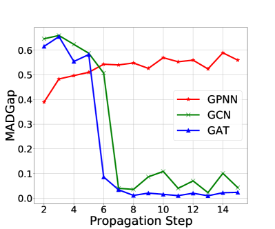
(a) MADGap

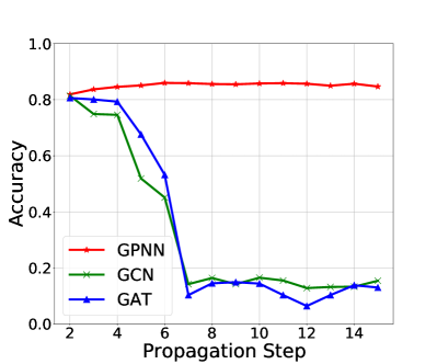
(b) Accuracy

Figure 3: Over-smoothing analysis on Cora in terms of MADGap and accuracy w.r.t. different propagation steps.

As is shown in Figure 3, when models are shallow, although the MADGap value of GPNN is smaller than that of GCN and GAT, our model achieves a higher classification accuracy on Cora. This phenomenon indicates that moderate smoothness of node embeddings can improve performance on classification. Meanwhile, when the propagation step increases to 6, the MADGap and classification accuracy of GCN and GAT drop rapidly while these two metrics of GPNN remain stable and get promoted slightly. We can conclude that GPNN is robust to over-smoothing, which we attribute to the well-designed parameters sharing MLP partner and the consistency contrastive loss. Additionally, by removing transformation in the middle graph convolution layers, GPNN significantly raises the lower bound of the Dirichlet energy which indicates a clear mitigation of the over-smoothing issue. Detailed analysis is provided in the Appendix.

6.4 Ablation Study

We investigate the contributions of each component from the perspective of improving model performance and relieving over-smoothing.

Graph Partner and Rectification Loss

In this part, we take a deeper insight into the contributions of both the proposed graph partner and the rectification loss. Since both of these two components cannot directly influence the learning of the embedding matrix $\mathbf{H}^{(l+1)}$,

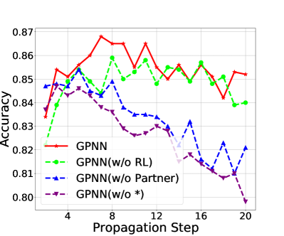
(a) Cora

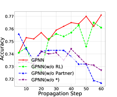
(b) Citeseer

Figure 4: Accuracy w.r.t. to different propagation steps on Cora and Citeseer. GPNN(w/o) RL corresponds to GPNN without rectification loss. GPNN(w/o Partner) represents that only use GCN for prediction. GPNN(w/o *) corresponds to GPNN without both graph Partner and rectification loss.

we analyze their effects from how the performance changes when the propagation step continuously increases. From Figure4, we observe that the blue line declines faster when the propagation step increases while the red line stays more stable and a huge gap exists between them. This result suggests that graph partner is especially useful for tackling over-smoothing and improving accuracy. We attribute this quality to the essence of MLP for preserving the feature of the node itself. Furthermore, the rectification loss has a slight positive effect on performance but it seems that rectification loss does not help relieve over-smoothing. In practice, when the training process reaches a certain number of epochs, the rectification loss remains almost unchanged, which may mean that the model has reached a balance point for boosting the two branches learning from each other and classifying nodes.

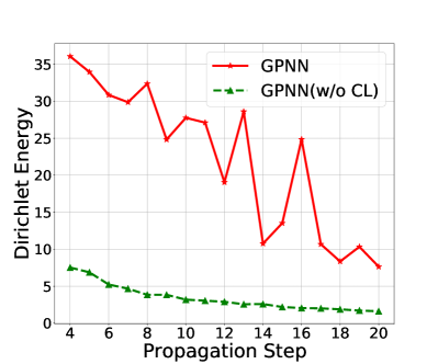
(a) Dirichlet Energy

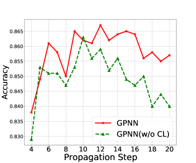
(b) Accuracy

Figure 5: Dirichlet energy of $\mathbf{H}^{(l+1)}$ and accuracy on Cora w.r.t. different propagation steps. GPNN(w/o CL) corresponds to GPNN without contrastive loss.

Consistency Contrastive Loss

We investigate the contributions of the consistency contrastive loss by analyzing the effect it puts upon $\mathbf{H}^{(l+1)}$ since it’s directly applied on $\mathbf{H}^{(l+1)}$. Recall that an extremely small Dirichlet energy reveals that the model is severely suffering from over-smoothing. We make two observations from Figure 5: 1) The red line is consistently higher than the green line in Figure 5(a), which indicates that the proposed consistency contrastive loss significantly raises the Dirichlet energy of $\mathbf{H}^{(l+1)}$, thus making the nodes better separated in the embedding space. 2) As the number of layers increases, the Dirichlet energy gradually drops, but the accuracy first rises and then declines. This further confirms the experimental conclusion we have drawn that proper smoothness of node embeddings can improve performance.

Table 3: Average cosine similarity and average same-label rate statistics for original edges and newly added edges by graph enhancement with $t=0.4$. We only list the statistics on Cora, Pubmed, and Coauthor CS due to space limitation. The rest is provided in the Appendix. Rate corresponds to average same-label rate, similarity corresponds to average cosine similarity, - represents the results of the originally connected node pairs and * represents the results of the newly connected node pairs. Acc. corresponds to accuracy. Acc.(w/o En) corresponds to accuracy of GPNN without graph enhancement.

Metric	Cora	Pubmed	Coauthor CS
Rate-	81.0	80.2	80.8
Rate*	90.1	78.3	90.2
Similarity-	0.17	0.27	0.40
Similarity*	0.53	0.50	0.49
Acc.(w/o En)	85.5 ± 0.5	80.4 ± 0.4	92.2 ± 0.3
Acc.	86.0 ± 0.4	80.8 ± 0.4	93.1 ± 0.5

Impact of Graph Enhancement

The enhanced graph encodes both structure and attribute information and makes the connections (edges) denser. We empirically analyze its impact on learning representations from the perspective of connection quality and model performance. We adopt the average cosine similarity and average same-label rate over all the connected node pairs to quantitatively measure the quality of connections. The same-label rate is defined as the proportion of nodes of the same class in all the first-order neighbors. Chen et al. (2020a) conducted experiments to prove that even with the same model and propagation step, nodes with higher same-label rate (which they call information-to-noise ratio) generally have higher prediction accuracy. Table 3 lists the average cosine similarity and average same-label rates of the original connections and new connections added by graph enhancement on Cora, Pubmed, and Coauthor CS. As one can see, new connections have high quality in terms of similarity and same-label rate, which indicates that graph enhancement can detect new connections that generally have better quality compared with the original edges. Graph enhancement is especially useful for Coauthor CS and Citeseer, and not very beneficial to other datasets. We speculate that the improvement of performance is highly correlated to the dataset itself. For example, graph enhancement can greatly improve the quality and amount of the connections for Coauthor CS and thus leads to a significant performance improvement.

Table 4: Efficiency comparison of GPNN with GCNII (wall time, in secs., average values of 10 runs). The results include all the time overhead (including the computation time of graph enhancement).

Dataset	GCNII	GPNN
Cora	94.9	10.9($8.71\times$)
CiteSeer	48.8	31.5($1.55\times$)
PubMed	20.7	37.3($0.55\times$)
Coauthor CS	171.6	65.4($2.62\times$)
A-Computer	79.8	10.1($7.90\times$)
A-Photo	152.7	9.7($15.74\times$)

6.5 Training Efficiency Comparison

We compare GPNN with the most competitive deep model GCNII on training efficiency. For a fair comparison, we implement GCNII with the official code (https://github.com/chennnM/GCNII) and adopt their original hyperparameters for Cora, Citeseer, and Pubmed, while tuning better hyperparameters for the other three datasets since no records are available in the original paper. We conduct experiments with a machine running Ubuntu 20.04LTS with two Intel Xeon Gold 6240L CPUs, one 32GB NVIDIA V100 GPU, and 256GB Memory. From Table 4 we notice that GPNN takes less time to converge than that of GCNII on 5 out of 6 datasets. In particular, GPNN has a large advantage over GCNII with speedup $15.74\times$ on Amazon-Photo. Another worth noting point is that GPNN has much fewer parameters compared with GCNII, which means less memory usage.

7 Conclusion

In this paper, we propose GPNN, a simple method for training deep models. GPNN consists of a de-parameterized GCN and a parameters-sharing MLP partner. We further leverage contrastive learning and consistency regularization to ensure the consistency between representations of different times and of different learning branches. we also propose a graph enhancement technique for improving the connection quality. Experimental results show that GPNN outperforms the state-of-the-art baselines on various semi-supervised node classification tasks. Besides, extensive experiments are conducted to investigate the contributions of each component and show efficiency advantage over GCNII, the most powerful deep model in the literature.

References

- Bachman et al. [2019] Philip Bachman, R. Devon Hjelm, and William Buchwalter. Learning representations by maximizing mutual information across views. In NeurIPS, pages 15509–15519, 2019.
- Belkin et al. [2006] Mikhail Belkin, Partha Niyogi, and Vikas Sindhwani. Manifold regularization: A geometric framework for learning from labeled and unlabeled examples. J. Mach. Learn. Res., 7:2399–2434, 2006.
- Cai and Wang [2020] Chen Cai and Yusu Wang. A note on over-smoothing for graph neural networks. arXiv preprint arXiv:2006.13318, 2020.
- Chen et al. [2020a] Deli Chen, Yankai Lin, Wei Li, Peng Li, Jie Zhou, and Xu Sun. Measuring and relieving the over-smoothing problem for graph neural networks from the topological view. In AAAI, pages 3438–3445. AAAI Press, 2020.
- Chen et al. [2020b] Ming Chen, Zhewei Wei, Zengfeng Huang, Bolin Ding, and Yaliang Li. Simple and deep graph convolutional networks. In ICML, volume 119 of Proceedings of Machine Learning Research, pages 1725–1735. PMLR, 2020.
- Chen et al. [2020c] Ting Chen, Simon Kornblith, Mohammad Norouzi, and Geoffrey E. Hinton. A simple framework for contrastive learning of visual representations. In ICML, volume 119 of Proceedings of Machine Learning Research, pages 1597–1607. PMLR, 2020.
- Chung and Graham [1997] Fan RK Chung and Fan Chung Graham. Spectral graph theory. Number 92. American Mathematical Soc., 1997.
- Defferrard et al. [2016] Michaël Defferrard, Xavier Bresson, and Pierre Vandergheynst. Convolutional neural networks on graphs with fast localized spectral filtering. In NIPS, pages 3837–3845, 2016.
- Deng et al. [2020] Chenhui Deng, Zhiqiang Zhao, Yongyu Wang, Zhiru Zhang, and Zhuo Feng. Graphzoom: A multi-level spectral approach for accurate and scalable graph embedding. In ICLR. OpenReview.net, 2020.
- Hammond et al. [2011] David K Hammond, Pierre Vandergheynst, and Rémi Gribonval. Wavelets on graphs via spectral graph theory. Applied and Computational Harmonic Analysis, 30(2):129–150, 2011.
- Hassani and Ahmadi [2020] Kaveh Hassani and Amir Hosein Khas Ahmadi. Contrastive multi-view representation learning on graphs. In ICML, volume 119 of Proceedings of Machine Learning Research, pages 4116–4126. PMLR, 2020.
- He et al. [2020] Xiangnan He, Kuan Deng, Xiang Wang, Yan Li, Yong-Dong Zhang, and Meng Wang. Lightgcn: Simplifying and powering graph convolution network for recommendation. In SIGIR, pages 639–648. ACM, 2020.
- Hinton et al. [2015] Geoffrey Hinton, Oriol Vinyals, and Jeff Dean. Distilling the knowledge in a neural network. arXiv preprint arXiv:1503.02531, 2015.
- Khosla et al. [2020] Prannay Khosla, Piotr Teterwak, Chen Wang, Aaron Sarna, Yonglong Tian, Phillip Isola, Aaron Maschinot, Ce Liu, and Dilip Krishnan. Supervised contrastive learning. arXiv preprint arXiv:2004.11362, 2020.
- Kipf and Welling [2017] Thomas N. Kipf and Max Welling. Semi-supervised classification with graph convolutional networks. In ICLR (Poster). OpenReview.net, 2017.
- Klicpera et al. [2018] Johannes Klicpera, Aleksandar Bojchevski, and Stephan Günnemann. Predict then propagate: Graph neural networks meet personalized pagerank. arXiv preprint arXiv:1810.05997, 2018.
- Klicpera et al. [2019] Johannes Klicpera, Aleksandar Bojchevski, and Stephan Günnemann. Predict then propagate: Graph neural networks meet personalized pagerank. In ICLR (Poster). OpenReview.net, 2019.
- Li et al. [2018] Ruoyu Li, Sheng Wang, Feiyun Zhu, and Junzhou Huang. Adaptive graph convolutional neural networks. In AAAI, pages 3546–3553. AAAI Press, 2018.
- Oono and Suzuki [2020] Kenta Oono and Taiji Suzuki. Graph neural networks exponentially lose expressive power for node classification. In ICLR. OpenReview.net, 2020.
- Qiu et al. [2020] Jiezhong Qiu, Qibin Chen, Yuxiao Dong, Jing Zhang, Hongxia Yang, Ming Ding, Kuansan Wang, and Jie Tang. GCC: graph contrastive coding for graph neural network pre-training. In KDD, pages 1150–1160. ACM, 2020.
- Rong et al. [2020] Yu Rong, Wenbing Huang, Tingyang Xu, and Junzhou Huang. Dropedge: Towards deep graph convolutional networks on node classification. In ICLR. OpenReview.net, 2020.
- Sen et al. [2008] Prithviraj Sen, Galileo Namata, Mustafa Bilgic, Lise Getoor, Brian Galligher, and Tina Eliassi-Rad. Collective classification in network data. AI magazine, 29(3):93–93, 2008.
- Shchur et al. [2018] Oleksandr Shchur, Maximilian Mumme, Aleksandar Bojchevski, and Stephan Günnemann. Pitfalls of graph neural network evaluation. arXiv preprint arXiv:1811.05868, 2018.
- Tian et al. [2020] Yonglong Tian, Dilip Krishnan, and Phillip Isola. Contrastive multiview coding. In ECCV (11), volume 12356 of Lecture Notes in Computer Science, pages 776–794. Springer, 2020.
- Velickovic et al. [2018] Petar Velickovic, Guillem Cucurull, Arantxa Casanova, Adriana Romero, Pietro Liò, and Yoshua Bengio. Graph attention networks. In ICLR (Poster). OpenReview.net, 2018.
- Velickovic et al. [2019] Petar Velickovic, William Fedus, William L. Hamilton, Pietro Liò, Yoshua Bengio, and R. Devon Hjelm. Deep graph infomax. In ICLR (Poster). OpenReview.net, 2019.
- Verma et al. [2021] Vikas Verma, Meng Qu, Kenji Kawaguchi, Alex Lamb, Yoshua Bengio, Juho Kannala, and Jian Tang. Graphmix: Improved training of gnns for semi-supervised learning. In AAAI, pages 10024–10032. AAAI Press, 2021.
- Wan et al. [2021] Sheng Wan, Shirui Pan, Jian Yang, and Chen Gong. Contrastive and generative graph convolutional networks for graph-based semi-supervised learning. In AAAI, pages 10049–10057. AAAI Press, 2021.
- Wang et al. [2020] Xiao Wang, Meiqi Zhu, Deyu Bo, Peng Cui, Chuan Shi, and Jian Pei. AM-GCN: adaptive multi-channel graph convolutional networks. In KDD, pages 1243–1253. ACM, 2020.
- Wu et al. [2019] Felix Wu, Amauri H. Souza Jr., Tianyi Zhang, Christopher Fifty, Tao Yu, and Kilian Q. Weinberger. Simplifying graph convolutional networks. In ICML, volume 97 of Proceedings of Machine Learning Research, pages 6861–6871. PMLR, 2019.
- Wu et al. [2021] Zonghan Wu, Shirui Pan, Fengwen Chen, Guodong Long, Chengqi Zhang, and Philip S. Yu. A comprehensive survey on graph neural networks. IEEE Trans. Neural Networks Learn. Syst., 32(1):4–24, 2021.
- Xu et al. [2018] Keyulu Xu, Chengtao Li, Yonglong Tian, Tomohiro Sonobe, Ken-ichi Kawarabayashi, and Stefanie Jegelka. Representation learning on graphs with jumping knowledge networks. In ICML, volume 80 of Proceedings of Machine Learning Research, pages 5449–5458. PMLR, 2018.
- Yang et al. [2016] Zhilin Yang, William W. Cohen, and Ruslan Salakhutdinov. Revisiting semi-supervised learning with graph embeddings. In ICML, volume 48 of JMLR Workshop and Conference Proceedings, pages 40–48. JMLR.org, 2016.
- Zhang et al. [2018] Hongyi Zhang, Moustapha Cissé, Yann N. Dauphin, and David Lopez-Paz. mixup: Beyond empirical risk minimization. In ICLR (Poster). OpenReview.net, 2018.
- Zhou et al. [2003] Dengyong Zhou, Olivier Bousquet, Thomas Navin Lal, Jason Weston, and Bernhard Schölkopf. Learning with local and global consistency. In NIPS, pages 321–328. MIT Press, 2003.
- Zhou et al. [2021] Kaixiong Zhou, Xiao Huang, Daochen Zha, Rui Chen, Li Li, Soo-Hyun Choi, and Xia Hu. Dirichlet energy constrained learning for deep graph neural networks. arXiv preprint arXiv:2107.02392, 2021.
- Zhu et al. [2003] Xiaojin Zhu, Zoubin Ghahramani, and John D. Lafferty. Semi-supervised learning using gaussian fields and harmonic functions. In ICML, pages 912–919. AAAI Press, 2003.
- Zhu et al. [2020] Yanqiao Zhu, Yichen Xu, Feng Yu, Qiang Liu, Shu Wu, and Liang Wang. Deep graph contrastive representation learning. arXiv preprint arXiv:2006.04131, 2020.