Projected Model Counting: Beyond Independent Support

Abstract

The past decade has witnessed a surge of interest in practical techniques for projected model counting. Despite significant advancements, however, performance scaling remains the Achilles’ heel of this field. A key idea used in modern counters is to count models projected on an independent support that is often a small subset of the projection set, i.e. original set of variables on which we wanted to project. While this idea has been effective in scaling performance, the question of whether it can benefit to count models projected on variables beyond the projection set, has not been explored. In this paper, we study this question and show that contrary to intuition, it can be beneficial to project on variables beyond the projection set. In applications such as verification of binarized neural networks, quantification of information flow, reliability of power grids etc., a good upper bound of the projected model count often suffices. We show that in several such cases, we can identify a set of variables, called upper bound support (UBS), that is not necessarily a subset of the projection set, and yet counting models projected on UBS guarantees an upper bound of the true projected model count. Theoretically, a UBS can be exponentially smaller than the smallest independent support. Our experiments show that even otherwise, UBS-based projected counting can be more efficient than independent support-based projected counting, while yielding bounds of very high quality. Based on extensive experiments, we find that UBS-based projected counting can solve many problem instances that are beyond the reach of a state-of-the-art independent support-based projected model counter.

1 Introduction

Given a Boolean formula $\varphi$ over a set $X$ of variables, and a subset $P$ of $X$, the problem of projected model counting requires us to determine the number of satisfying assignments of $\varphi$ projected on $\mathcal{P}$. Projected model counting is # NP-complete in general [35], and has several important applications ranging from verification of neural networks [6], hardware and software verification [34], reliability of power grids [13], probabilistic inference [26, 27, 15], and the like. Not surprisingly, the problem has attracted attention from both theoreticians and practitioners over the years [36, 32, 19, 9, 11, 30, 29]. In particular, there has been recent strong interest in techniques that scale in practice and also provide provable guarantees on the quality of computed counts.

Over the past decade, hashing-based techniques have emerged as a promising approach to projected model counting, since they scale relatively well in practice, while also providing strong approximation guarantees [19, 8, 9, 15, 24]. The core idea of hashing-based projected model counting is to partition the projected solution space into roughly equal small cells such that one can estimate the projected model count or sample projected solutions uniformly by picking a random cell. The practical implementation of these techniques rely on the use of random XOR clauses constructed from variables in the projection set $\mathcal{P}$. Starting with a CNF formula $\varphi$, we therefore end up with a conjunction of CNF and XOR clauses, also referred to as a CNF+XOR formula, that must be fed to a backend SAT solver. The standard construction of a random XOR clause selects each variable in $\mathcal{P}$ for inclusion in the clause with probability $1/2$; hence the expected clause size is $|\mathcal{P}|/2$. Unfortunately, the performance of modern SAT solvers on CNF+XOR formulas is heavily impacted by the sizes of XOR clauses [17, 10, 37]. This explains why designing hash functions with sparse XOR clauses is important in scaling hashing-based projected model counting [17, 15, 14, 5, 20, 2, 1, 23].

A practically effective idea to address the aforementioned problem was introduced in [10], wherein the notion of an independent support was introduced in the context of (projected) model counting. Informally, a set $\mathcal{I}\subseteq\mathcal{P}$ is an independent support of $\mathcal{P}$ if whenever two projected solutions of $\varphi$ agree on the values of variables in $\mathcal{I}$, they also agree on the values of all variables in $\mathcal{P}$. It was shown in [10] that random XOR clauses over the independent support suffice to provide all desired theoretical guarantees [10]. Furthermore, for benchmarks arising in practice, $|\mathcal{I}|$ was found to be often much smaller than $|\mathcal{P}|$. Hence, using $\mathcal{I}$ instead of $\mathcal{P}$ in the construction of random XOR clauses improved the runtime performance of hashing-based approximate (projected) counters and samplers, often by several orders of magnitude [20]. Subsequently, independent supports have also been found to be useful in the context of exact (projected) model counting [22, 28].

The runtime performance improvements achieved by (projected) model counters over the past decade have significantly broadened the scope of their applications, which, in turn, has brought the focus sharply back on performance scalability. Importantly, for several important applications such as neural network verification [6], quantified information flow [7], software reliability [34], reliability of power grids [13], etc. we are primarily interested in good upper bound estimates of projected model counts. As apty captured by Achlioptas and Theodoropoulos [2], while obtaining “lower bounds are easy” in the context of projected model counting, such is not the case for good upper bounds. Therefore, scaling up to large problem instances while obtaining good upper bound estimates remains an important challenge in this area.

The primary contribution of this paper is a new approach to selecting variables on which to project solutions, with the goal of improving scalability of hashing-based projected counters when good upper bounds of projected counts are of interest. Towards this end, we generalize the notion of an independent support $\mathcal{I}$. Specifically, we note that the restriction $\mathcal{I}\subseteq\mathcal{P}$ ensures a two-way implication: if two solutions agree on $\mathcal{I}$, then they also agree on $\mathcal{P}$, and vice-versa. Since we are interested in upper bounds, we relax this requirement to a one-sided implication, i.e., we wish to find a set $\mathcal{U}\subseteq X$ (not necessarily a subset of $\mathcal{P})$ such that if two solutions agree on $\mathcal{U}$, then they agree on $\mathcal{\mathcal{P}}$, but not necessarily vice versa. We call such a set $\mathcal{U}$ an Upper Bound Support, or UBS for short. We show that using random XOR clauses over UBS in hashing-based projected counting yields provable upper bounds of the projected counts. We also show some important properties of UBS, including an exponential gap between the smallest UBS and the smallest independent support for a class of problems. Our study suggests a simple iterative algorithm, called FindUBS, to determine UBS, that can be fine-tuned heuristically.

To evaluate the effectiveness of our idea, we augment a state-of-the-art model counter, ApproxMC4, with UBS to obtain UBS+ApproxMC4. Through an extensive empirical evaluation on $2632$ benchmark instances arising from diverse domains, we compare the performance of UBS+ApproxMC4 with IS+ApproxMC4, i.e. ApproxMC4 augmented with independent support computation. Our experiments show that UBS+ApproxMC4 is able to solve 208 more instances than IS+ApproxMC4. Furthermore, the geometric mean of the absolute value of log-ratio of counts returned by UBS+ApproxMC4 and IS+ApproxMC4 is 1.32, thereby validating the claim that using UBS can lead to empirically good upper bounds. In this context, it is worth remarking that a recent study [3] comparing different partition function estimation techniques labeled a method with the absolute value of log-ratio of counts less than 5 as a reliable method.

The rest of the paper is organized as follows. We present notation and preliminaries in Section 2. To situate our contribution, we present a survey of related work in Section 3. We then present the primary technical contributions of our work, including the notion of UBS and an algorithmic procedure to determine UBS, in Section 4. We present our empirical evaluation in Section 5, and finally conclude in Section 6.

2 Notation and Preliminaries

Let $X=\{x_{1},x_{2}\ldots x_{n}\}$ be a set of propositional variables appearing in a propositional formula $\varphi$. The set $X$ is called the support of $\varphi$, and denoted $\mathsf{Sup}({\varphi})$. A literal is either a propositional variable or its negation. The formula $\varphi$ is said to be in Conjunctive Normal Form (CNF) if $\varphi$ is a conjunction of clauses, where each clause is disjunction of literals. An assignment $\sigma$ of $X$ is a mapping $X\rightarrow\{0,1\}$. If $\varphi$ evaluates to $1$ under assignment $\sigma$, we say that $\sigma$ is a model or satisfying assignment of $\varphi$, and denote this by $\sigma\models\varphi$. For every $\mathcal{P}\subseteq X$, the projection of $\sigma$ on $\mathcal{P}$, denoted ${\sigma}_{\downarrow{{\mathcal{P}}}}$, is a mapping $\mathcal{P}\rightarrow\{0,1\}$ such that ${\sigma}_{\downarrow{{\mathcal{P}}}}(v)=\sigma(v)$ for all $v\in\mathcal{P}$. Conversely we say that an assignment $\widehat{\sigma}:\mathcal{P}\rightarrow\{0,1\}$ can be extended to a model of $\varphi$ if there exists a model $\sigma$ of $\varphi$ such that $\widehat{\sigma}={\sigma}_{\downarrow{{\mathcal{P}}}}$. The set of all models of $\varphi$ is denoted $sol({\varphi})$, and the projection of this set on $\mathcal{P}\subseteq X$ is denoted $sol({\varphi})_{\downarrow{\mathcal{P}}}$. We call the set $\mathcal{P}$ a projection set in our subsequent discussion.

The problem of projected model counting is to compute $|sol({\varphi})_{\downarrow{\mathcal{P}}}|$ for a given CNF formula $\varphi$ and projection set $\mathcal{P}$. An exact projected model counter is a deterministic algorithm that takes $\varphi$ and $\mathcal{P}$ as inputs and returns $|sol({\varphi})_{\downarrow{\mathcal{P}}}|$ as output. A probably approximately correct (or $\mathsf{PAC}$) projected model counter is a probabilistic algorithm that takes as additional inputs a tolerance $\varepsilon>0$, and a confidence parameter $\delta\in(0,1]$, and returns a count $c$ such that $\mathsf{Pr}\Big{[}\frac{|sol({\varphi})_{\downarrow{\mathcal{P}}}|}{(1+\varepsilon)}\leq c\leq(1+\varepsilon)\cdot|sol({\varphi})_{\downarrow{\mathcal{P}}}|\Big{]}\geq 1-\delta$, where $\mathsf{Pr}[E]$ denotes the probability of event $E$.

Definition 1

Given a formula $\varphi$ and a projection set $\mathcal{P}\subseteq\mathsf{Sup}({\varphi})$, a subset of variables $\mathcal{I}\subseteq\mathcal{P}$ is called an independent support (IS) of $\mathcal{P}$ in $\varphi$ if for every $\sigma_{1},\sigma_{2}\in sol({\varphi})$, we have $\big{(}{\sigma_{1}}_{\downarrow{{\mathcal{I}}}}={\sigma_{2}}_{\downarrow{{\mathcal{I}}}}\big{)}\Rightarrow\big{(}{\sigma_{1}}_{\downarrow{{\mathcal{P}}}}={\sigma_{2}}_{\downarrow{{\mathcal{P}}}}\big{)}$.

Since $\big{(}{\sigma_{1}}_{\downarrow{{\mathcal{P}}}}={\sigma_{2}}_{\downarrow{{\mathcal{P}}}}\big{)}\Rightarrow\big{(}{\sigma_{1}}_{\downarrow{{\mathcal{I}}}}={\sigma_{2}}_{\downarrow{{\mathcal{I}}}}\big{)}$ holds trivially when $\mathcal{I}\subseteq\mathcal{P}$, it follows from Definition 1 that if $\mathcal{I}$ is an independent support of $\mathcal{P}$ in $\varphi$, then $\big{(}{\sigma_{1}}_{\downarrow{{\mathcal{I}}}}={\sigma_{2}}_{\downarrow{{\mathcal{I}}}}\big{)}\Leftrightarrow\big{(}{\sigma_{1}}_{\downarrow{{\mathcal{P}}}}={\sigma_{2}}_{\downarrow{{\mathcal{P}}}}\big{)}$. Empirical studies have shown that the size of an independent support $\mathcal{I}$ is often significantly smaller than that of the original projection set $\mathcal{P}$ [10, 20, 22, 28]. This has been exploited successfully in the design of practically efficient $\mathsf{PAC}$ hashing-based model counters like ApproxMC4 [29]. Specifically, the overhead of finding a small independent support $\mathcal{I}$ is often more than compensated by the efficiency obtained by counting projections of satisfying assignments on $\mathcal{I}$, instead of on the original projection set $\mathcal{P}$.

3 Background

State-of-the-art hashing-based projected model counters work by randomly partitioning the projected solution space of a given CNF formula into roughly equal small “cells”, followed by counting and suitably scaling the number of projected solutions in a randomly picked cell. The random partitioning is usually achieved using specialized hash functions, implemented by adding random XOR clauses to the given CNF formula. There are several inter-related factors that affect the scalability of such hashing-based model counters, and isolating the effect of any one factor on performance is extremely difficult. Nevertheless, finding satisfying assignments of the CNF+XOR formula has been empirically found to be the most significant bottleneck. The difficulty of solving such a formula depends not only on the original CNF formula, but also on the random XOR clauses that are added to it. Specifically, the average size (i.e. number of literals) in the added XOR clauses is known to correlate positively with the time taken to solve CNF+XOR formulas using modern conflict-driven clause learning (CDCL) SAT solvers [20]. This has motivated interesting research that aims to reduce the average size of XOR clauses added to a given CNF formula in the context of hashing-based approximate model counting [10, 5, 15, 14, 2, 1, 23].

The idea of using random XOR clauses over an independent support $\mathcal{I}$ that is potentially much smaller than the projection set $\mathcal{P}$ was first introduced in [10]. This is particularly effective when a small subset of variables functionally determines the large majority of variables in a formula, as happens, for example, when Tseitin encoding is used to transform a non-CNF formula to an equisatisfiable CNF formula. State-of-the-art hashing-based model counters, viz. ApproxMC4 [29], therefore routinely use random XOR clauses over the independent support. While the naive way of choosing each variable in $\mathcal{I}$ with probability $1/2$ gives a random XOR clause with expected size $|\mathcal{I}|/2$, researchers have also explored whether specialized hash functions can be defined over $\mathcal{I}$ such that the expected size of a random XOR clause is $p\cdot|\mathcal{I}|$, with $p<1/2$ [5, 15, 14, 2, 1, 23]. The works of [5, 15, 14, 2, 1] achieved this goal while guaranteeing a constant factor approximation of the reported count. The work of [23] achieved a similar reduction in the expected size of XOR clauses, while guaranteeing PAC-style bounds. The latter work also turns out to be more scalable in practice.

While earlier work focused on independent supports that are necessarily subsets of the projection set $\mathcal{P}$, we break free from this restriction and allow any subset of variables in the construction of random XOR clauses as long as the model count projected on the chosen subset bounds the model count projected on $\mathcal{P}$ from above. This gives us more flexibility in constructing CNF+XOR formulas, which as our experiments confirm, leads to improved overall performance of projected model counting in several cases. Since we guarantee upper bounds of the desired counts, theoretically, our approach yields an upper bounding projected model counter. Nevertheless, as our experiments show, the bounds obtained using our approach are consistently very close to the projected counts reported using independent support. Therefore, in practice, our approach gives high quality bounds on projected model counts more efficiently than state-of-the-art hashing-based techniques that use independent supports.

It is worth mentioning here that several bounding model counters have been reported earlier in the literature. These counters report a count that is at least as large (or, as small, as the case may be) as the true model count of the given CNF formula with a given confidence. Notable examples of such counters are SampleCount [18], BPCount [21], MBound and Hybrid-MBound [19] and MiniCount [21]. Owing to several technical reasons, however, these bounding counters do not scale as well as state-of-the-art hashing-based counters like ApproxMC4 [29] in practice. Unlike earlier bounding counters, we first carefully identify an upper bound set, and then use state-of-the-art hashing-based approximate projected counting, while treating the computed upper bound set as the new projection set. Therefore, our approach directly benefits from significant improvements in performance of hashing-based projected counting achieved over the years. Moreover, by carefully controlling the set of variables over which the upper bound set is computed, we can also control the quality of the bound. For example, if the upper bound set is chosen entirely from within the projection set, then the upper bound set can be shown to be an independent support. In this case, the counts reported by our approach truly have PAC-style guarantees.

4 Technical Contribution

In this section, we generalize the notion of independent support, and give technical details of projected model counting using this generalization. We start with some definitions.

Definition 2

Given a CNF formula $\varphi$ and a projection set $\mathcal{P}$, let $\mathcal{S}\subseteq\mathsf{Sup}({\varphi})$ be such that for every $\sigma_{1},\sigma_{2}\in sol({\varphi})$, we have $\big{(}{\sigma_{1}}_{\downarrow{{\mathcal{S}}}}={\sigma_{2}}_{\downarrow{{\mathcal{S}}}}\big{)}~{}\bowtie~{}\big{(}{\sigma_{1}}_{\downarrow{{\mathcal{P}}}}={\sigma_{2}}_{\downarrow{{\mathcal{P}}}}\big{)}$, where $\bowtie~{}\in\{\Rightarrow,\Leftarrow,\Leftrightarrow\}$. Then $\mathcal{S}$ is called a

1. generalized independent support (GIS) of $\mathcal{P}$ in $\varphi$ if $\bowtie$ is  $\Leftrightarrow$

2. upper bound support (UBS) of $\mathcal{P}$ in $\varphi$ if $\bowtie$ is  $\Rightarrow$

3. lower bound support (LBS) of $\mathcal{P}$ in $\varphi$ if $\bowtie$ is  $\Leftarrow$

Note that in the above definition, $\mathcal{S}$ need not be a subset of $\mathcal{P}$. In fact, if $\mathcal{S}$ is restricted to be a subset of $\mathcal{P}$, the definitions of GIS and UBS coincide with that of IS (Definition 1), while LBS becomes a trivial concept (every subset of $\mathcal{P}$ is indeed an LBS of $\mathcal{P}$ in $\varphi$). The following lemma now follows immediately.

Lemma 1

Let $\mathcal{G}$, $\mathcal{U}$ and $\mathcal{L}$ be GIS, UBS and LBS, respectively, of $\mathcal{P}$ in $\varphi$. Then $|sol({\varphi})_{\downarrow{\mathcal{L}}}|\leq|sol({\varphi})_{\downarrow{\mathcal{P}}}|$ $=|sol({\varphi})_{\downarrow{\mathcal{G}}}|$ $\leq|sol({\varphi})_{\downarrow{\mathcal{U}}}|$.

Let $\mathcal{UBS},\mathcal{LBS},\mathcal{GIS}$ and $\mathcal{IS}$ be the set of all UBS, LBS, GIS and IS respectively of a projection set $\mathcal{P}$ in $\varphi$. It follows from the above definitions that $\mathcal{IS}\subseteq\mathcal{GIS}\subseteq\mathcal{UBS}$, and $\mathcal{GIS}\subseteq\mathcal{LBS}$. While each of the notions of GIS, UBS and LBS are of independent interest, this paper focuses primarily on UBS for varios reasons. First, we found this notion to be particularly useful in practical projected model counting. Additionally, as the above inclusion relations show, $\mathcal{UBS}$ and $\mathcal{LBS}$ are the largest classes among $\mathcal{UBS},\mathcal{LBS},\mathcal{GIS}$ and $\mathcal{IS}$; hence, finding an UBS is likely to be easier than finding a GIS. Furthermore, the notion of UBS continues to remain interesting (but not so for LBS, as mentioned above) even when $\mathcal{I}$ is chosen to be a subset of $\mathcal{P}$.

We call a UBS $\mathcal{U}$ (resp. LBS $\mathcal{L}$, GIS $\mathcal{G}$ and IS $\mathcal{I}$) of $\mathcal{P}$ in $\varphi$ minimal if there is no other UBS (resp. LBS, GIS and IS) of $\mathcal{P}$ in $\varphi$ of size/cardinality strictly less than $|\mathcal{U}|$ (resp. $|\mathcal{L}|$, $|\mathcal{G}|$ and $|\mathcal{I}|$). Minimal UBS are useful for computing good upper bounds of projected model counts, since they help reduce the size of random XOR clauses used in hashing-based projected model counting.

In the remainder of this section, we first explore some interesting theoretical properties of GIS and UBS, and then proceed to develop a practical algorithm for computing an UBS from a given formula $\varphi$ and projection set $\mathcal{P}$. Finally, we present an algorithm for computing bounds of projected model counts using the UBS thus computed.

4.1 Extremal properties of GIS and UBS

We first show that relaxing the requirement that variables on which to project models must be chosen from the projection set can lead to an exponential improvement in the size of the independent/upper-bound support.

Theorem 4.1

For every $n>1$, there exists a propositional formula $\varphi_{n}$ on $(n-1)+\lceil\log_{2}n\rceil$ variables and a projection set $\mathcal{P}_{n}$ with $|\mathcal{P}_{n}|=n-1$ such that

• The smallest GIS of $\mathcal{P}_{n}$ in $\varphi_{n}$ is of size $\lceil\log_{2}n\rceil$.

• The smallest UBS of $\mathcal{P}_{n}$ in $\varphi_{n}$ is of size $\lceil\log_{2}n\rceil$.

• The smallest IS of $\mathcal{P}_{n}$ in $\varphi_{n}$ is $\mathcal{P}_{n}$ itself, and hence of size $n-1$.

Proof: For notational convenience, we assume $n$ to be a power of $2$. Consider a formula $\varphi_{n}$ on $(n-1)+\log_{2}n$ propositional variables $x_{1},\ldots x_{n-1},$ $y_{1},\ldots y_{\log_{2}n}$ with $n$ satisfying assignments, say $\sigma_{0},\ldots\sigma_{n-1}$, as shown in the table below.

	$x_{1}$	$x_{2}$	$\cdots$	$x_{n-1}$	$y_{1}$	$y_{2}$	$\cdots$	$y_{\log_{2}n}$
$\sigma_{0}$	$0$	$0$	$\cdots$	$0$	$0$	$\cdots$	$0$	$0$
$\sigma_{1}$	$1$	$0$	$\cdots$	$0$	$0$	$\cdots$	$0$	$1$
$\sigma_{2}$	$0$	$1$	$\cdots$	$0$	$0$	$\cdots$	$1$	$0$
	$\vdots$	$\vdots$	$\vdots$	$\vdots$	$\vdots$	$\vdots$	$\vdots$	$\vdots$
$\sigma_{n-1}$	$0$	$0$	$\cdots$	$1$	$1$	$\cdots$	$1$	$1$

Thus, for all $i\in\{1,\ldots n-1\}$, the values of $y_{1}\ldots y_{log_{2}n}$ in $\sigma_{i}$ encode the number $i$ in binary (with $y_{\log_{2}n}$ being the least significant bit, and $y_{1}$ being the most significant bit), the value of $x_{i}$ is $1$, and the values of all other $x_{j}$’s are $0$. For the special satisfying assignment $\sigma_{0}$, the values of all variables are $0$.

Let $\mathcal{P}_{n}=\{x_{1},\ldots x_{n-1}\}$. Clearly, $|sol({\varphi_{n}})|=|sol({\varphi_{n}})_{\downarrow{\mathcal{P}_{n}}}|=n$. Now consider the set of variables $\mathcal{G}_{n}=\{y_{1},\ldots y_{\log_{2}n}\}$. It is easy to verify that for every pair of satisfying assignments $\sigma_{i},\sigma_{j}$ of $\varphi_{n}$, $\big{(}{\sigma_{i}}_{\downarrow{{\mathcal{G}_{n}}}}={\sigma_{j}}_{\downarrow{{\mathcal{G}_{n}}}}\big{)}\Leftrightarrow\big{(}{\sigma_{i}}_{\downarrow{{\mathcal{P}_{n}}}}={\sigma_{j}}_{\downarrow{{\mathcal{P}_{n}}}}\big{)}$. Therefore, $\mathcal{G}_{n}$ is a GIS, and hence also a UBS, of $\mathcal{P}_{n}$ in $\varphi_{n}$, and $|\mathcal{G}_{n}|=\log_{2}n$. Indeed, specifying $y_{1},\ldots y_{\log_{2}n}$ completely specifies the value of all variables for every satisfying assignment of $\varphi_{n}$. Furthermore, since $|sol({\varphi_{n}})_{\downarrow{\mathcal{P}_{n}}}|=n$, every GIS and also UBS of $\mathcal{P}_{n}$ must be of size at least $\log_{2}n$. Hence, $\mathcal{G}_{n}$ is a smallest-sized GIS, and also a smallest-sized UBS, of $\mathcal{P}_{n}$ in $\varphi_{n}$.

Let us now find how small an independent support (IS) of $\mathcal{P}_{n}$ in $\varphi$ can be. Recall that $|sol({\varphi_{n}})_{\downarrow{\mathcal{P}_{n}}}|=n$. If possible, let there be an IS of $\mathcal{P}_{n}$, say $\mathcal{I}_{n}\subseteq\mathcal{P}_{n}$, where $|\mathcal{I}_{n}|<n-1$. Therefore, at least one variable in $\mathcal{P}_{n}$, say $x_{i}$, must be absent in $\mathcal{I}_{n}$. Now consider the satisfying assignments $\sigma_{i}$ and $\sigma_{0}$. Clearly, both ${\sigma_{i}}_{\downarrow{{\mathcal{I}_{n}}}}$ and ${\sigma_{0}}_{\downarrow{{\mathcal{I}_{n}}}}$ are the all-$0$ vector of size $n-1$. Therefore, ${\sigma_{i}}_{\downarrow{{\mathcal{I}_{n}}}}={\sigma_{0}}_{\downarrow{{\mathcal{I}_{n}}}}$ although ${\sigma_{i}}_{\downarrow{{\mathcal{P}_{n}}}}\neq{\sigma_{0}}_{\downarrow{{\mathcal{P}_{n}}}}$. It follows that $\mathcal{I}_{n}$ cannot be an IS of $\mathcal{P}_{n}$ in $\varphi_{n}$. This implies that the smallest IS of $\mathcal{P}_{n}$ in $\varphi_{n}$ is $\mathcal{P}_{n}$ itself, and has size $n-1$. ∎

Observe that the smallest GIS/UBS $\mathcal{G}_{n}$ in the above proof is disjoint from $\mathcal{P}_{n}$. This suggests that it can be beneficial to look outside the projection set when searching for a compact GIS or UBS. The next theorem shows that the opposite can also be true.

Theorem 4.2 ()

For every $n>1$, there exist propositional formulas $\varphi_{n}$ and $\psi_{n}$ on $(n-1)+\lceil\log_{2}n\rceil$ variables and a projection set $\mathcal{Q}_{n}$ with $|\mathcal{Q}_{n}|=n-\lceil\log_{2}n\rceil-2$ such that the only GIS of $\mathcal{Q}_{n}$ in $\varphi_{n}$ is $\mathcal{Q}_{n}$, and the smallest UBS of $\mathcal{Q}_{n}$ in $\psi_{n}$ is also $\mathcal{Q}_{n}$.

Proof: We assume $n$ to be a power of $2$ and consider the same formula $\varphi_{n}$ as used in the proof of Theorem 4.1. We use $\sigma_{0},\ldots\sigma_{n-1}$ to denote the satisfying assignments of $\varphi_{n}$, as before. Additionally, we choose $\psi_{n}$ to be the formula on the same set of variables and with the same number ($n$) of satisfying assignments, say $\widehat{\sigma_{0}},\ldots\widehat{\sigma_{n-1}}$, defined as follows: for all $i\in\{0,\ldots n-1\}$, $\widehat{\sigma_{i}}(x_{j})=\sigma_{i}(x_{j})$ for $j\in\{1,\ldots n-1\}$, and $\widehat{\sigma_{i}}(y_{j})=0$ for $j\in\{1,\ldots\log_{2}n\}$. In other words, all $y_{j}$’s are set to $0$ in all satisfying assignments of $\psi_{n}$. We also choose $\mathcal{Q}_{n}=\{x_{1},\ldots x_{n-1}\}\setminus\{x_{2^{0}},x_{2^{1}},\ldots x_{n/2}\}$. Thus, $|\mathcal{Q}_{n}|=(n-1)-\lceil\log_{2}n\rceil-1$ $=n-\lceil\log_{2}n\rceil-2$.

Let $\mathcal{G}_{n}$ be a generalized independent support (GIS) of $\mathcal{Q}_{n}$ in $\varphi_{n}$. We state and prove below some auxiliary claims that help in proving the main result.

Claim 1: $\forall i\in\{0\ldots\log_{2}n-1\}$,   ${\sigma_{0}}_{\downarrow{{\mathcal{Q}_{n}}}}={\sigma_{2^{i}}}_{\downarrow{{\mathcal{Q}_{n}}}}$.
Indeed, both ${\sigma_{0}}_{\downarrow{{\mathcal{Q}_{n}}}}$ and ${\sigma_{2^{i}}}_{\downarrow{{\mathcal{Q}_{n}}}}$ are the all-$0$ vectors of length $|\mathcal{Q}_{n}|$.

Claim 2: $\forall i\in\{1,\ldots\log_{2}n\}$,   $y_{i}\not\in\mathcal{G}_{n}$.
To see why this is so, let us express $i$ as $\log_{2}n-j$, where $j\in\{0,\ldots\log_{2}n-1\}$. Then, it is easy to see that $y_{i}=0$ in $\sigma_{0}$ and $y_{i}=1$ in $\sigma_{2^{j}}$. However, from Claim 1, we know that ${\sigma_{0}}_{\downarrow{{\mathcal{Q}_{n}}}}={\sigma_{2^{j}}}_{\downarrow{{\mathcal{Q}_{n}}}}$. Since $\mathcal{G}_{n}$ is a GIS of $\mathcal{Q}_{n}$, by properties of GIS, we cannot have $y_{i}\in\mathcal{G}_{n}$.

Claim 3: $\forall i\in\{0,\ldots\log_{2}n-1\}$,   $x_{2^{i}}\not\in\mathcal{G}_{n}$.
By a similar reasoning as above, we see that $x_{2^{i}}=0$ in $\sigma_{0}$ and $x_{2^{i}}=1$ in $\sigma_{2^{i}}$. Therefore, since $\mathcal{G}_{n}$ is a GIS of $\mathcal{Q}_{n}$, from Claim 1, we cannot have $x_{2^{i}}\in\mathcal{G}_{n}$.

Claim 4: $\forall x_{j}\in\mathcal{Q}_{n}$,   $x_{j}\in\mathcal{G}_{n}$.
To see why this is so, suppose $x_{j}\not\in\mathcal{G}_{n}$, and let $\mathcal{Q}_{n}^{\prime}=\mathcal{Q}_{n}\setminus\{x_{j}\}$. From Claims 2 and 3 above, we must then have $\mathcal{G}_{n}\subseteq\mathcal{Q}_{n}^{\prime}$. Hence, $\mathcal{Q}_{n}^{\prime}$ must be an IS of $\mathcal{Q}_{n}$ in $\varphi_{n}$. However, note that ${\sigma_{0}}_{\downarrow{{\mathcal{Q}_{n}^{\prime}}}}={\sigma_{j}}_{\downarrow{{\mathcal{Q}_{n}^{\prime}}}}$ although ${\sigma_{0}}_{\downarrow{{\mathcal{Q}_{n}}}}\neq{\sigma_{j}}_{\downarrow{{\mathcal{Q}_{n}}}}$. Therefore, $\mathcal{Q}_{n}^{\prime}$ cannot be an IS of $\mathcal{Q}_{n}$ in $\varphi_{n}$ – a contradiction! Therefore, $x_{j}$ must be in $\mathcal{G}_{n}$.

Putting Claims 1 through 4 together, $\mathcal{Q}_{n}$ is the only GIS of $\mathcal{Q}_{n}$ in $\varphi_{n}$.

Next, we show that the smallest UBS of $\mathcal{Q}_{n}$ in $\psi_{n}$ is $\mathcal{Q}_{n}$. Let $\mathcal{U}_{n}$ be an UBS of $\mathcal{Q}_{n}$ in $\psi_{n}$ such that there is no smaller (cardinality-wise) UBS of $\mathcal{Q}_{n}$ in $\psi_{n}$.

Claim 5: $\forall i\in\{1,\ldots\log_{2}n\}$,   $y_{i}\not\in\mathcal{U}_{n}$.
This follows from the observation that $y_{i}=0$ in every $\widehat{\sigma_{j}}$ for $j\in\{0\ldots n-1\}$. Thus, if $\mathcal{U}_{n}$ is a UBS of $\mathcal{Q}_{n}$ in $\psi_{n}$ and if $y_{i}\in\mathcal{U}_{n}$, then $\mathcal{U}_{n}\setminus\{y_{i}\}$ must also be a UBS of $\mathcal{Q}_{n}$ in $\psi_{n}$. This contradicts the fact that there is no other UBS of cardinality less than $|\mathcal{U}_{n}|$.

Claim 6: $\forall x_{j}\in\mathcal{Q}_{n}$,   $x_{j}\in\mathcal{U}_{n}$.
To see why this is so, suppose $x_{j}\not\in\mathcal{U}_{n}$ and let $\mathcal{U}_{n}^{\prime}=\{x_{1},\ldots x_{n-1}\}\setminus\{x_{j}\}$. From Claim 5 above, we must then have $\mathcal{U}_{n}\subseteq\mathcal{U}_{n}^{\prime}$. However, note that ${\widehat{\sigma_{0}}}_{\downarrow{{\mathcal{U}_{n}^{\prime}}}}={\widehat{\sigma_{j}}}_{\downarrow{{\mathcal{U}_{n}^{\prime}}}}$ although ${\widehat{\sigma_{0}}}_{\downarrow{{\mathcal{Q}_{n}}}}\neq{\widehat{\sigma_{j}}}_{\downarrow{{\mathcal{Q}_{n}}}}$. Therefore, $\mathcal{U}_{n}^{\prime}$ cannot be a UBS of $\mathcal{Q}_{n}$ in $\psi_{n}$. Since $\mathcal{U}_{n}\subseteq\mathcal{U}_{n}^{\prime}$, it follows that $\mathcal{U}_{n}$ cannot be a UBS of $\mathcal{Q}_{n}$ in $\psi_{n}$ either.

Putting Claims 5 and 6 together, the smallest UBS of $\mathcal{Q}_{n}$ in $\psi_{n}$ is $\mathcal{Q}_{n}$ itself. ∎

Theorems 4.1 and 4.2 show that when searching for a compact GIS or UBS, we may have to consider all possibilities, ranging from staying within the projection set to being completely disjoint from the projection set.

4.2 An algorithm to compute UBS

We now describe an algorithm to compute a UBS for a given CNF formula $\varphi$ and projection set $\mathcal{P}$. We draw our motivation from Padoa’s theorem [25], which provides a necessary and sufficient condition to determine when a variable in the support of a formula $\varphi$ is functionally determined by the other variables in the support. Without loss of generality, let $\mathsf{Sup}({\varphi})=X=\{x_{1},x_{2},\ldots x_{t}\}$. We create another set of fresh variables ${X^{\prime}}=\{x_{1}^{\prime},x_{2}^{\prime},\ldots x_{t}^{\prime}\}$. Let $\varphi(X\mapsto{X^{\prime}})$ represent the formula where every $x_{i}\in X$ in $\varphi$ is replaced by $x_{i}^{\prime}\in{X^{\prime}}$. In the following, we write $\varphi(X)$ to clarify that the support of $\varphi$ is $X$.

Lemma 2 (Padoa’s Theorem [25])

Let $\psi(X,{X^{\prime}},i)$ be defined as $\varphi(X)\wedge\varphi(X\mapsto{X^{\prime}})\wedge\bigwedge_{j=1\atop{j\neq i}}^{t}(x_{j}\Leftrightarrow x_{j}^{\prime})\wedge x_{i}\wedge\neg x_{i}^{\prime}$. The variable $x_{i}$ is defined by $X\setminus\{x_{i}\}$ in the formula $\varphi$ iff $\psi(X,{X^{\prime}},i)$ is unsatisfiable.

Padoa’s theorem has been effectively used in state-of-the-art hashing-based projected model counters such as ApproxMC4 [29] to determine small independent supports of given projection sets. In our setting, we need to modify the formulation since we seek to compute an upper bound support.

Given the projection set $\mathcal{P}$, we first partition the support $X$ of $\varphi$ into three sets as follows:

• $J$: the set of variables already determined to be in a minimal UBS of $\mathcal{P}$ in $\varphi$

• $Q$: the set of variables for which we do not know yet if they are in a minimal UBS of $\mathcal{P}$ in $\varphi$

• $D$: the set of variables that need not appear in a minimal UBS of $\mathcal{P}$ in $\varphi$ obtained by adding elements to $J$

Initially, $J$ and $D$ are empty sets, and $Q=X$. As the process of computation of a minimal UBS proceeds, we wish to maintain the invariant that $J\cup Q$ is a UBS (not necessarily minimal) of $\mathcal{P}$ in $\varphi$. Notice that this is true initially, since $X$ is certainly a UBS of $\mathcal{P}$ in $\varphi$.

Let $z$ be a variable in $Q$ for which we wish to determine if it needs to be added to the partially computed minimal UBS $J$. In the following discussion, we use the notation $\varphi(J,Q\setminus\{z\},D,z)$ to denote $\varphi$ with its partition of variables, and with $z$ specially identified in the partition $Q$. Recalling the definition of UBS from Section 2, we observe that if $z$ is not part of a minimal UBS obtained by augmenting $J$, and if $J\cup Q$ is indeed a UBS of $\mathcal{P}\in\varphi$, then as long as values other than $z$ in $J\cup Q$ are kept unchanged, the projection of a satisfying assignment of $\varphi$ on $\mathcal{P}$ must also stay unchanged. This suggests the following check to determine if $z$ is not part of a minimal UBS obtained by augmenting $J$.

Define $\xi(J,Q\setminus\{z\},D,z,D^{\prime},z^{\prime})$ as $\varphi(J,Q\setminus\{z\},D,z)\wedge\varphi(J,Q\setminus\{z\},D^{\prime},z^{\prime})\wedge\bigvee_{x_{i}~{}\in~{}\mathcal{P}\cap(D\cup\{z\})}(x_{i}\not\Leftrightarrow x_{i}^{\prime})$, where $D^{\prime}$ and $z^{\prime}$ represent fresh and renamed instances of variables in $D$ and $z$, respectively. If $\xi$ is unsatisfiable, we know that as long as the values of variables in $J\cup(Q\setminus\{z\})$ are kept unchanged, the projection of the satisfying assginment of $\varphi$ on $\mathcal{P}$ cannot change. This allows us to move $z$ from the set $Q$ to the set $D$.

Theorem 4.3 ()

If $\xi(J,Q\setminus\{z\},D,z,D^{\prime},z^{\prime})$ is unsatisfiable, then $J\cup(Q\setminus\{z\})$ is a UBS of $\mathcal{P}$ in $\varphi$.

Proof: Without loss of generality, assume that there are no primed variables in $J,Q$ and $D$. Let $J^{\prime}=\{x_{i}^{\prime}\mid x_{i}\in J\}$, and similarly for $Q^{\prime}$ and $D^{\prime}$. From the definition of UBS in Section 4, we know that $J\cup Q\setminus\{z\}$ is a UBS of $\mathcal{P}$ in $\varphi$ if the following formula is valid:

$$\Big{(}\varphi(J,Q\setminus z,D,z)\wedge\varphi(J^{\prime},Q^{\prime}\setminus z^{\prime},D^{\prime},z^{\prime})\wedge\bigwedge_{x_{i}\in(J\cup Q\setminus z)}(x_{i}\Leftrightarrow x_{i}^{\prime})\Big{)}\Rightarrow\bigwedge_{x_{j}\in\mathcal{P}}(x_{j}\Leftrightarrow x_{j}^{\prime})$$

Note that $x_{i}\Leftrightarrow x_{i}^{\prime}$ is already asserted in the antecedent of the implication for all $x_{i}\in(J\cup Q\setminus z)$. Furthermore, variables in $J^{\prime}\cup Q^{\prime}\setminus z^{\prime}$ do not appear in the consequent of the above implication. Since the support of $\varphi$ is partitioned into $J,Q\setminus z,D$ and $\{z\}$, we also have $\mathcal{P}\setminus(J\cup Q\setminus z)~{}=~{}\mathcal{P}\cap(D\cup\{z\})$. Putting these facts together, the condition for $J\cup Q\setminus\{z\}$ to be a UBS reduces to validity of

$$\Big{(}\varphi(J,Q\setminus z,D,z)\wedge\varphi(J,Q\setminus z,D^{\prime},z^{\prime})\Big{)}\Rightarrow\bigwedge_{x_{j}\in\mathcal{P}\cap(D\cup\{z\})}(x_{j}\Leftrightarrow x_{j}^{\prime})$$

In other words, $J\cup Q\setminus\{z\}$ is a UBS of $\mathcal{P}$ in $\varphi$ if $\varphi(J,Q\setminus z,D,z)\wedge\varphi(J,Q\setminus z,D^{\prime},z^{\prime})\wedge\bigvee_{x_{j}\in\mathcal{P}\cap(D\cup\{z\})}(x_{j}\not\Leftrightarrow x_{j}^{\prime})$ is unsatisfiable.

∎

The above check suggests a simple algorithm for computing a minimal UBS. We present the pseudocode of our algorithm for computing UBS below.

1:$J\leftarrow\emptyset;Q\leftarrow\mathsf{Sup}({\varphi});D\leftarrow\emptyset$;

2:repeat

3:    $z\leftarrow\mathsf{ChooseNextVar}(Q)$;

4:    $\xi\leftarrow\left(\begin{array}[]{c}\varphi(J,Q\setminus z,D,z)~{}\wedge~{}\varphi(J,Q\setminus z,D^{\prime},z^{\prime})~{}\wedge\\ \bigvee_{x_{i}~{}\in~{}\mathcal{P}\cap(D\cup\{z\})}\neg(x_{i}\Leftrightarrow x_{i}^{\prime})\end{array}\right)$;

5:    if $\xi$ is $\mathsf{UNSAT}$ then

6:         $D\leftarrow D\cup\{z\}$;

7:    else

8:         $J\leftarrow J\cup\{z\}$;     

9:    $Q\leftarrow Q\setminus\{z\}$;

10:until $Q$ is $\emptyset$;

11:return $J$;

Algorithm 1 FindUBS$(\varphi,\mathcal{P})$

After initializing $J$, $Q$ and $D$, FindUBS chooses a variable $z\in Q$ and checks if the formula $\xi$ in Theorem 4.3 is unsatisfiable. If so, it adds $z$ to $D$ and removes it from $Q$. Otherwise, it adds $z$ to $J$. The algorithm terminates when $Q$ becomes empty. On termination, $J$ gives a minimal UBS of $\mathcal{P}$ in $\varphi$. The strategy for choosing the next $z$ from $Q$, implemented by sub-routine $\mathsf{ChooseNextVar}$, clearly affects the quality of UBS obtained from this algorithm. We require that $\mathsf{ChooseNextVar}(Q)$ return a variable from $Q$ as long as $Q\neq\emptyset$. Choosing $z$ from within $\mathcal{P}$ gives a UBS that is the same as an IS of $\mathcal{P}$ in $\varphi$. In our experiments, we therefore bias the choice of $z$ to favour those not in $\mathcal{P}$ when selecting variables from $Q$.

We now state some key properties of Algorithm FindUBS.

Lemma 3 ()

The following invariant holds at the loop head (line 2) of Algorithm 1: There exists a minimal UBS $\mathcal{U}^{*}$ of $\mathcal{P}$ in $\varphi$ such that $J\subseteq\mathcal{U}^{*}\subseteq J\cup Q$.

Proof

From the initialization of $J$ and $Q$ in line 1, we know that when Algorithm 1 reaches line 2 for the first time, $Q=\mathsf{Sup}({\varphi})$ and $J=\emptyset$. Since every minimal UBS of $\mathcal{P}$ in $\varphi$ must be contained in $\mathsf{Sup}({\varphi})$ and must contain $\emptyset$, it follows that the invariant is satisfied when the algorithm reaches line 2 for the first time.

Let us now inductively hypothesize that the invariant holds at the start of $k^{th}$ iteration of the repeat-until loop. There are two cases to consider in the inductive step.

• If the formula $\xi$ (see line 4 of Algorithm 1) is $\mathsf{UNSAT}$, then $J$ stays unchanged in the $k^{th}$ iteration. Furthermore, from Theorem 4.3, we know that $J\cup(Q\setminus\{z\})$ is an UBS of $\mathcal{P}$ in $\varphi$. This implies there is at least one minimal UBS that is a subset of $J(\cup Q\setminus\{z\})$. Since $z$ is removed from $Q$ in line 9, our proof would be complete if there exists a minimal UBS $\mathcal{U}^{*}$ such that $J\subseteq\mathcal{U}^{*}\subseteq(J\cup Q\setminus\{z\})$. Suppose, if possible, there is no such minimal UBS $\mathcal{U}^{*}$. From the inductive hypothesis, we also know that there exists at least one minimal UBS, say $\widehat{\mathcal{U}^{*}}$, such that $J\subseteq\widehat{\mathcal{U}^{*}}\subseteq(J\cup Q)$. The above assertions imply that $z$ must be present in every minimal UBS $\widehat{\mathcal{U}^{*}}$ that satisfies $J\subseteq\widehat{\mathcal{U}^{*}}\subseteq(J\cup Q)$. This, in turn, implies that $\varphi(J,Q\setminus z,D,z)\wedge\varphi(J,Q\setminus z,D^{\prime},z^{\prime})\not\Rightarrow\bigwedge_{x_{i}~{}\in~{}\mathcal{P}\cap(D\cup\{z\})}(x_{i}\Leftrightarrow x_{i}^{\prime})$. This contradicts the assumption that the formula $\xi$ is $\mathsf{UNSAT}$. Hence, our assumption must be incorrect, and there exists a minimal UBS $\mathcal{U}^{*}$ such that $J\subseteq\mathcal{U}^{*}\subseteq(J\cup Q\setminus\{z\})$.

  Therefore, the invariant holds at the loop head at the start of the $k+1^{st}$ iteration of the loop.

• Let $\sigma$ be a satisfying assignment of $\xi$. In this case, the variable $z$ is removed from $Q$ and added to $J$ in lines 8 and 9; hence $J\cup Q$ stays unchanged.

  The assignment of values to variables in $\sigma$ yields two satisfying assignments of $\varphi$ that agree on the values of variables in $J\cup(Q\setminus{z})$, and yet the projections of the satisfying assignments on $\mathcal{P}$ are different. Therefore, $J\cup(Q\setminus\{z\})$ is not a UBS of $\mathcal{P}$ in $\varphi$. Since every superset of a UBS is also a UBS (easy consequence of the definition of UBS), this implies that there is no minimal UBS that is contained in $J\cup(Q\setminus\{z\})$. However, we know from the inductive hypothesis that there is at least one minimal UBS, say $\mathcal{U}^{*}$, such that $J\subseteq\mathcal{U}^{*}\subseteq J\cup Q$. The above two assertions imply that $z\in\mathcal{U}^{*}$. Hence, $(J\cup\{z\})\subseteq\mathcal{U}^{*}\subseteq(J\cup\{z\})\cup(Q\setminus\{z\})$.

  Once again, the invariant holds at the loop head at the start of the $k+1^{st}$ iteration of the loop.

Theorem 4.4 ()

Algorithm 1, when invoked on $\varphi$ and $\mathcal{P}$, terminates and computes a minimal UBS of $\mathcal{P}$ in $\varphi$.

Proof

In line 1 of Algorithm 1, the set $Q$ is initialized with $\mathsf{Sup}({\varphi})$, which has finitely many variables. Subsequently, in each iteration of the repeat-until loop in lines 2–10, exactly one variable is removed from $Q$, and no other variable is added to $Q$. Therefore, $Q$ must become empty after $|\mathsf{Sup}({\varphi})|$ iterations of the loop, leading to termination of Algorithm 1.

Let $J^{*}$ and $Q^{*}$ denote the values of $J$ and $Q$, respectively, on termination. From Lemma 3, we know that there is a minimal UBS $\mathcal{U}^{*}$ of $\mathcal{P}$ in $\varphi$ such that $J^{*}\subseteq\mathcal{U}^{*}\subseteq J^{*}\cup Q^{*}$. However, $Q^{*}=\emptyset$ on termination of the algorithm. Hence $J^{*}=\mathcal{U}^{*}$, and Algorithm 1 terminates with a minimal UBS of $\mathcal{P}$ in $\varphi$.

The overall algorithm for computing an upper bound of the projected model count of a CNF formula using UBS is shown in Algorithm 2. This algorithm takes two timeout parameters, $\tau_{\mathrm{pre}}$ and $\tau_{\mathrm{count}}$. These are used to limit the times taken for computing a UBS using algorithm FindUBS, and for computing a projected model count of $\varphi$ on the computed UBS, respectively.

Algorithm 2 $\mathsf{UBCount}$$(\varphi,\mathcal{P},\varepsilon,\delta,\tau_{\mathrm{pre}},\tau_{\mathrm{count}})$

1:$\mathcal{U}\leftarrow$ FindUBS$(\varphi,\mathcal{P})$ with timeout $\tau_{\mathrm{pre}}$;

2:if call to FindUBS times out then

3:    $\mathcal{U}\leftarrow\mathcal{P}$;

4:return $\mathsf{ComputeCount}(\varphi,\mathcal{U},\varepsilon,\delta)$

Theorem 4.5 ()

Given a CNF formula $\varphi$, a projection set $\mathcal{P}$, parameters $\varepsilon~{}(>0)$ and $\delta~{}(0<\delta<1)$, and given access to a PAC counter, $\mathsf{ComputeCount}$, suppose Algorithm 2 returns a count $c$. Then for every choice of $\mathsf{ChooseNextVar}$, we have $\mathsf{Pr}\left[{|sol({\varphi})_{\downarrow{\mathcal{P}}}|\leq(1+\varepsilon)\cdot c}\right]\geq 1-\delta$.

Proof

From Theorem 4.4, we know that when Algorithm 2 reaches line 4, the set $\mathcal{U}$ is a UBS of $\mathcal{P}$ in $\varphi$. Hence $|sol({\varphi})_{\downarrow{\mathcal{P}}}|\leq|sol({\varphi})_{\downarrow{\mathcal{U}}}|$. Furthermore, since $\mathsf{ComputeCount}$ is a PAC counter, we have $\mathsf{Pr}\left[{\frac{|sol({\varphi})_{\downarrow{\mathcal{U}}}|}{1+\varepsilon}\leq c\leq(1+\varepsilon)\cdot|sol({\varphi})_{\downarrow{\mathcal{U}}}|}\right]$ $\geq 1-\delta$. The theorem now follows easily from the above two observations.

Theorem 4.5 provides the weakest guarantee for Algorithm $\mathsf{UBCount}$, ignoring the details of sub-routine $\mathsf{ChooseNextVar}$. In practice, the specifics of $\mathsf{ChooseNextVar}$ can be factored in to strengthen the guarantee, including providing PAC-style guarantees in the extreme case if $\mathsf{ChooseNextVar}$ always chooses variables from the projection set $\mathcal{P}$. A more detailed analysis of $\mathsf{UBCount}$, taking into account the specifics of $\mathsf{ChooseNextVar}$ is beyond the scope of this paper.

5 Experimental Evaluation

To evaluate practical efficiency of $\mathsf{UBCount}$, we implemented a prototype in C++. Our prototype implementation builds on $\mathsf{Arjun}$ [31]. To demonstrate practical impact of computation of UBS on model counting, we first compute UBS and pass the UBS as a projection set along with the formula $\varphi$ to the state of the art hashing-based approximate counter ApproxMC4 [29].

We chose ApproxMC4 because it is a highly competitive projected model counter, a version of which won the 2020 model counting competition in the projected counting track. In this context, it is worth remarking that the 2021 competition sought to focus on the exact counters (which do not rely on hashing-based methods) and consequently, changed required $\varepsilon=0.1$ to $\varepsilon=0.01$. Since the complexity of approximate techniques has $\varepsilon^{-2}$ dependence, this led to nearly 100$\times$ penalty in runtime for the approximate techniques. Even then, ApproxMC4-based entry achieved 3rd place. As described during the competitive event presentation at the SAT 2021, had $\varepsilon$ been set to $0.05$, the ApproxMC4-based entry would have won the competition. All prior applications and benchmarking for approximation techniques have been presented with $\varepsilon=0.8$ in the literature, and we continue to use the same value of $\varepsilon$ in this work.

We use UBS+ApproxMC4 to denote the case when ApproxMC4 is invoked with the computed UBS as the projection set while we use IS+ApproxMC4 to refer to the version of ApproxMC4 invoked with IS as the projection set.

Benchmarks

Our benchmark suite consisted of 2632 instances, which are categorized into four categories: BNN, Circuit, QBF-exist and QBF-circuit. BNN benchmarks are adapted from [6]. Each instance contains CNF encoding of binarized neural networks (BNN) and constraints from properties of interest such as robustness, cardinality, and parity. The projection set $\mathcal{P}$ is set to variables for a chosen layer. The class ‘Circuit’ refers to instances from [10], which encode circuits arising from ISCAS benchmarks conjuncted with random parity constraints imposed on output variables. The projection set, as set by authors in [10], corresponds to output variables. The benchmarks with ‘QBF’ are based on instances from Prenex-2QBF track of QBFEval-17, QBFEval-18, disjunctive [4], arithmetic [33] and factorization [4]. Each ‘QBF-exist’ benchmark is a CNF formula transformed from a QBF instance. We remove quantifiers for the (2-)QBF instance and set the projection set to existentially quantified variables. The class ‘QBF-circuit’ refers to circuits synthesized using the state of the art functional synthesis tool, Manthan [16]. The projection set is set to output variables.

Experiments were conducted on a high-performance computer cluster, each node consisting of 2xE5-2690v3 CPUs with 2x12 real cores and 96GB of RAM. The model counter with per preprocessing technique on a particular benchmark runs on a single core. We set the time limit as 5000 seconds for preprocessing and counting respectively and the memory limit as 4GB. The maximal number of conflicts is 100k for each candidate variable during preprocessing. To compare runtime performance, we employ PAR-2 scores, which is a standard in SAT community, in the context of SAT competition. Each benchmark contributes a score that is the number of seconds used by the corresponding tool to successfully finish the execution or in case of a timeout or memory out, twice the timeout in seconds. We then calculate the average score for all benchmarks, giving PAR-2.

We sought to answer the following research questions:

RQ 1

Does the usage of UBS enable ApproxMC4 to solve more benchmarks in comparison to the usage of IS ?

RQ 2

How does the quality of counts computed by UBS+ApproxMC4 vary in comparison to IS+ApproxMC4?

RQ 3

How does the runtime behavior of UBS+ApproxMC4 compare with that of IS+ApproxMC4?

Summary

In summary, UBS+ApproxMC4 solves 208 more instances than IS+ApproxMC4. Furthermore, while computation of UBS takes 777 more seconds, the PAR-2 score of UBS+ApproxMC4 is 817 seconds less than that of IS+ApproxMC4. Finally, for all the instances where both UBS+ApproxMC4 and IS+ApproxMC4 terminated the geometric mean of log-ratio of counts returned by IS+ApproxMC4 and UBS+ApproxMC4 is 1.32, therefore, indicating that UBS+ApproxMC4 provides accurate estimates and therefore, can be used as substitute for IS+ApproxMC4 in the context of applications that primarily care about upper bounds.

In this context, it is worth highlighting that since there has been considerable effort in recent years in the optimizing computation of IS, one would expect that further engineering efforts would lead to even more saving in runtime in the usage of UBS.

5.1 Number of Solved Benchmarks

Benchmarks	Total	VBS	IS+ApproxMC4	UBS+ApproxMC4
BNN	1224	868	823	823
Circuit	522	455	407	435
QBF-exist	607	314	156	291
QBF-circuit	279	152	100	145

Table 1: The number of solved benchmarks.

Table 1 compares the number of solved benchmarks by IS+ApproxMC4 and UBS+ApproxMC4. Observe that the usage of UBS enables ApproxMC4 to solve 435, 291, and 145 instances on Circuit, QBF-exist, and QBF-circuit benchmark sets respectively while the usage of IS+ApproxMC4 solved 407, 156 and 100 instances. In particular, UBS+ApproxMC4 solved almost twice as many instances on QBF-exist benchmarks.

The practical adoption of tools for NP-hard problems often rely on portfolio solvers. Therefore, from the perspective of practice, one is often interested in evaluating the impact of a new technique to the portfolio of existing state of the art. To this end, we often focus on Virtual Best Solver (VBS), which can be viewed as an ideal portfolio. An instance is considered to be solved by VBS if is solved by at least one solver in the portfolio; that is, VBS is at least as powerful as each solver in the portfolio. Observe that on BNN benchmarks, while UBS+ApproxMC4 and IS+ApproxMC4 solved the same number of instances but VBS solves 45 more instances as there were 45 instances that were solved by UBS+ApproxMC4 but not IS+ApproxMC4.

5.2 Time Analysis

To analyze the runtime behavior, we separate the preprocessing time (computation of UBS and IS) and the time taken by ApproxMC4. Table 2 reports the mean of preprocessing time over benchmarks and the PAR-2 score for counting time. The usage of UBS reduces the PAR-2 score for counting from from 3680, 2206, 7493, and 6479 to 3607, 1766, 5238, and 4829 on four benchmark sets, respectively. Remarkably, UBS reduces PAR-2 score by over 2000 seconds on QBF-exist benchmarks and over 1000 seconds on QBF-circuit, which is a significant improvement.

	Preprocessing time		PAR-2 score of counting time
Benchmarks	0000IS (s)0000	0000UBS (s)0000	0000IS (s)0000	0000UBS (s)0000
BNN	2518	2533	3680	3607
Circuit	0229	0680	2206	1766
QBF-exist	0070	2155	7493	5238
QBF-circuit	0653	2541	6479	4829

Table 2: The mean of preprocessing time and PAR-2 score of counting time

Observe that the mean time taken by UBS is higher than that of IS across all four benchmark classes. Such an observation may lead one to wonder whether savings due to UBS are indeed useful; in particular, one may argue that if the total time of IS+ApproxMC4 is set to 10,000 seconds so that the time remaining after IS computation can be used by ApproxMC4. We observe that even in such a case, IS+ApproxMC4 is able to solve only four more instances than Table 1. To further emphasize, UBS+ApproxMC4 where ApproxMC4 is allowed a timeout of 5000 seconds can still solve more instance than IS+ApproxMC4 where ApproxMC4 is allowed a timeout of $10,000-t_{IS}$ where $t_{IS}$ is time taken to compute IS with a timeout of 5000 seconds.

Detailed Runtime Analysis

IS+ApproxMC4 UBS+ApproxMC4 Benchmarks $|X|$ $|\mathcal{P}|$ $|\text{{IS}}|$ Time (s) Count $|\text{{{UBS}}}|$ Time (s) Count amba2c7n.sat 1380 1345 313 0.24+2853 $50*2^{65\hphantom{00}}$ 73 0017+1000 $63*2^{67\hphantom{0}}$ bobtuint31neg 1634 1205 678 0.37+5000 $-$ 417 0148+1600 $64*2^{411}$ ly2-25-bnn_32-bit-5-id-11 131 32 32 1313+3416 $94*2^{9\hphantom{000}}$ 59 2113+1034 $63*2^{10\hphantom{0}}$ ly3-25-bnn_32-bit-5-id-10 131 32 32 1389+5000 $-$ 61 2319+8410 $60*2^{9\hphantom{00}}$ floor128 891 879 254 0.07+5000 $-$ 256 0009+6000 $64*2^{250}$ s15850_10_10.cnf 10985 684 605 0.50+5000 $-$ 600 0041+2070 $50*2^{566}$ arbiter_10_5 23533 129 118 0.71+4000 $64*2^{112\hphantom{0}}$ 302 0007+5000 $-$ cdiv_10_5 101705 128 60 0102+5000 $72*2^{50\hphantom{00}}$ $-$ 5000+5000 $-$ rankfunc59_signed_64 5140 4505 1735 0003+274 $43*2^{1727}$ $-$ 5000+5000 $-$

Table 3: Performance comparison of UBS vs. IS. The runtime is reported in seconds and “$-$’ in a column reports timeout after 5000 seconds.

Table 3 presents the results over a subset of benchmarks. Column 1 of the table gives the benchmark name, while columns 2 and 3 list the size of support $X$ and the size of projection set $\mathcal{P}$, respectively. Columns 4-6 list the size of computed IS, runtime of IS+ApproxMC4, and model count over IS while columns 7-9 correspond to UBS. Note that the time is represented in the form $t_{p}+t_{c}$ where $t_{p}$ refers to the time taken by IS (resp. UBS) and $t_{c}$ refers to the time taken by ApproxMC4. We use ‘$-$’ in column 6 (resp. column 9) for the cases where IS+ApproxMC4 (resp. UBS+ApproxMC4) times out. For example, on benchmark amba2c7n.sat, the computation of IS takes 0.24 seconds and returns an independent support of size 313 variables while the computation of UBS takes 17 seconds and the computed UBS has 73 variables. Furthermore, ApproxMC4 when supplied with IS takes 2853 seconds while ApproxMC4 with UBS takes only one second. The model count returned by ApproxMC4 in case of IS is $50*2^{65}$ while the count returned by ApproxMC4 in case of UBS is $63*2^{67}$.

The benchmark set was chosen to showcase different behaviors of interest: First, we observe that the smaller size of UBS for amba2c7n.sat leads UBS+ApproxMC4 while IS+ApproxMC4 times out. It is, however, worth emphasizing that the size of UBS and IS is not the only factor. To this end, observe that for the two benchmarks arising from BNN, represented in the third and fourth row, even though the size of UBS is large, the runtime of ApproxMC4 is still improved. Furthermore, in comparison to IS, our implementation for UBS did not explore engineering optimization, which shows how UBS computation times out in the presence of the large size of support. Therefore, an important direction of future research is to further optimize the computation of UBS to fully unlock the potential of UBS.

5.3 Quality of Upper Bound

To evaluate the quality of upper bound, we compare the counts computed by UBS+ApproxMC4 with those of IS+ApproxMC4 for 1376 instances where both IS+ApproxMC4 and UBS+ApproxMC4 terminated. Suppose $C_{\text{IS}}$ and $C_{\text{UBS}}$ denote the model count on IS and UBS respectively. The error $\mathsf{Error}$ is computed by $\mathsf{Error}=\log_{2}C_{\text{UBS}}-\log_{2}C_{\text{IS}}$. Figure 1 shows $\mathsf{Error}$ distribution over benchmarks. A point $(x,y)$ represents $\mathsf{Error}\leq y$ on the first $x$ benchmarks. For example, the point $(1000,2.2)$ means the $\mathsf{Error}$ is not more than 2.2 on one thousand benchmarks. Overall, the geometric mean of $\mathsf{Error}$ is just 1.32. Furthermore, for more than 67% benchmarks the $\mathsf{Error}$ is less than one, and for 81% benchmarks, the the $\mathsf{Error}$ is less than five while on only 11% benchmarks the $\mathsf{Error}$ is larger than ten. To put the significance of $\mathsf{Error}$ margin in the context, we refer to the recent survey [3] comparing several partition function estimation techniques, wherein a method with $\mathsf{Error}$ less than 5 is labeled as a reliable method. It is known that partition function estimate reduces to model counting, and the best performing technique identified in that study relies on model counting.

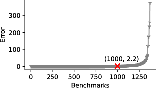
Figure 1: Error of upper bound.

6 Conclusion

In this work, we introduced the notion of Upper Bound Support (UBS), which generalizes the well-known notion of independent support. We then observed that the usage of UBS for generation of XOR constraints in the context of approximate projected model counting leads to the computation of upper bound of projected model counts. Our empirical analysis demonstrates that UBS+ApproxMC leads to significant runtime improvement in terms of the number of instances solved as well as the PAR-2 score. Since identification of the importance of IS in the context of counting led to follow-up work focused on efficient computation of IS, we hope our work will excite the community to work on efficient computation of UBS.

References

- [1] Achlioptas, D., Hammoudeh, Z., Theodoropoulos, P.: Fast and flexible probabilistic model counting. In: Proc. of SAT. pp. 148–164 (2018)
- [2] Achlioptas, D., Theodoropoulos, P.: Probabilistic model counting with short xors. In: Proc. of SAT. pp. 3–19 (2017)
- [3] Agrawal, D., Pote, Y., Meel, K.S.: Partition function estimation: A quantitative study. In: Proc. of IJCAI (8 2021)
- [4] Akshay, S., Chakraborty, S., John, A.K., Shah, S.: Towards parallel boolean functional synthesis. In: Proc. of TACAS. pp. 337–353 (2017)
- [5] Asteris, M., Dimakis, A.G.: Ldpc codes for discrete integration. Technical report, UT Austin (2016)
- [6] Baluta, T., Shen, S., Shine, S., Meel, K.S., Saxena, P.: Quantitative verification of neural networks and its security applications. In: Proc. of CCS (11 2019)
- [7] Biondi, F., Enescu, M., Heuser, A., Legay, A., Meel, K.S., Quilbeuf, J.: Scalable approximation of quantitative information flow in programs. In: Proc. of VMCAI (1 2018)
- [8] Chakraborty, S., Meel, K.S., Vardi, M.Y.: A scalable and nearly uniform generator of sat witnesses. In: Proc. of CAV. pp. 608–622 (7 2013)
- [9] Chakraborty, S., Meel, K.S., Vardi, M.Y.: A scalable approximate model counter. In: Proc. of CP. pp. 200–216 (9 2013)
- [10] Chakraborty, S., Meel, K.S., Vardi, M.Y.: Balancing scalability and uniformity in sat-witness generator. In: Proc. of DAC. pp. 60:1–60:6 (6 2014)
- [11] Chakraborty, S., Meel, K.S., Vardi, M.Y.: Algorithmic improvements in approximate counting for probabilistic inference: From linear to logarithmic SAT calls. In: Proc. of IJCAI (2016)
- [12] Chavira, M., Darwiche, A.: Compiling bayesian networks with local structure. In: IJCAI. vol. 5, pp. 1306–1312 (2005)
- [13] Duenas-Osorio, L., Meel, K.S., Paredes, R., Vardi, M.Y.: Counting-based reliability estimation for power-transmission grids. In: Proc. of AAAI (2 2017)
- [14] Ermon, S., Gomes, C., Sabharwal, A., Selman, B.: Low-density parity constraints for hashing-based discrete integration. In: Proc. of ICML. Proceedings of Machine Learning Research, vol. 32, pp. 271–279 (22–24 Jun 2014), https://proceedings.mlr.press/v32/ermon14.html
- [15] Ermon, S., Gomes, C.P., Sabharwal, A., Selman, B.: Taming the curse of dimensionality: Discrete integration by hashing and optimization. In: Proc. of ICML. JMLR Workshop and Conference Proceedings, vol. 28, pp. 334–342 (6 2013), http://proceedings.mlr.press/v28/ermon13.html
- [16] Golia, P., Roy, S., Meel, K.S.: Manthan: A data-driven approach for boolean function synthesis. In: Proc. of CAV (7 2020)
- [17] Gomes, C., Hoffmann, J., Sabharwal, A., Selman, B.: Short xors for model counting: From theory to practice. In: Proc. of SAT (2007)
- [18] Gomes, C., Hoffmann, J., Sabharwal, A., Selman, B.: From sampling to model counting. pp. 2293–2299 (01 2007)
- [19] Gomes, C.P., Sabharwal, A., Selman, B.: Model counting: A new strategy for obtaining good bounds. In: Proc. of AAAI. AAAI’06, vol. 1, p. 54–61 (2006)
- [20] Ivrii, A., Malik, S., Meel, K.S., Vardi, M.Y.: On computing minimal independent support and its applications to sampling and counting. Constraints 21(1) (9 2016)
- [21] Kroc, L., Sabharwal, A., Selman, B.: Leveraging belief propagation, backtrack search, and statistics for model counting. In: Proc. of CPAIOR. p. 127–141. CPAIOR’08 (2008)
- [22] Lagniez, J.M., Lonca, E., Marquis, P.: Improving model counting by leveraging definability. In: IJCAI. pp. 751–757 (2016)
- [23] Meel, K.S., Akshay, S.: Sparse hashing for scalable approximate model counting: Theory and practice. In: Proc. of LICS (7 2020)
- [24] Meel, K.S., Vardi, M.Y., Chakraborty, S., Fremont, D.J., Seshia, S.A., Fried, D., Ivrii, A., Malik, S.: Constrained sampling and counting: Universal hashing meets sat solving. In: Proc. of Workshop on BNP (2016)
- [25] Padoa, A.: Essai d’une théorie algébrique des nombres entiers, précédé d’une introduction logique à une théorie déductive quelconque. Bibliothèque du Congrès International de Philosophie 3, 309 (1901)
- [26] Roth, D.: On the hardness of approximate reasoning. Artificial Intelligence 82(1), 273–302 (1996). https://doi.org/https://doi.org/10.1016/0004-3702(94)00092-1, https://www.sciencedirect.com/science/article/pii/0004370294000921
- [27] Sang, T., Bearne, P., Kautz, H.: Performing bayesian inference by weighted model counting. In: Proc. of AAAI. AAAI’05, vol. 1, p. 475–481 (2005)
- [28] Sharma, S., Roy, S., Soos, M., Meel, K.S.: Ganak: A scalable probabilistic exact model counter. In: IJCAI. vol. 19, pp. 1169–1176 (2019)
- [29] Soos, M., Gocht, S., Meel, K.S.: Tinted, detached, and lazy cnf-xor solving and its applications to counting and sampling. In: Proc. of CAV (7 2020)
- [30] Soos, M., Meel, K.S.: Bird: Engineering an efficient cnf-xor sat solver and its applications to approximate model counting. In: Proc. of AAAI (1 2019)
- [31] Soos, M., Meel, K.S.: Arjun: An efficient independent support computation technique and its applications to counting and sampling. CoRR (2021)
- [32] Stockmeyer, L.: The complexity of approximate counting. In: Proc. of STOC. p. 118–126. STOC ’83 (1983). https://doi.org/10.1145/800061.808740, https://doi.org/10.1145/800061.808740
- [33] Tabajara, L.M., Vardi, M.Y.: Factored boolean functional synthesis. In: Proc. of FMCAD. p. 124–131. FMCAD ’17 (2017)
- [34] Teuber, S., Weigl, A.: Quantifying software reliability via model-counting. In: International Conference on Quantitative Evaluation of Systems. pp. 59–79. Springer (2021)
- [35] Valiant, L.G.: The complexity of computing the permanent. Theoretical Computer Science 8(2), 189–201 (1979)
- [36] Valiant, L.G.: The complexity of enumeration and reliability problems. SIAM Journal on Computing 8(3), 410–421 (1979). https://doi.org/10.1137/0208032, https://doi.org/10.1137/0208032
- [37] Zhao, S., Chaturapruek, S., Sabharwal, A., Ermon, S.: Closing the gap between short and long xors for model counting. In: Proc. of AAAI (2016)