Prosecutor Politics:
The Impact of Election Cycles on Criminal Sentencing in the Era of Rising Incarceration

I investigate how political incentives affect the behavior of district attorneys (DAs). I develop a theoretical model that predicts DAs will increase sentencing intensity in an election period compared to the period prior. To empirically test this prediction, I compile one of the most comprehensive datasets to date on the political careers of all district attorneys in office during the steepest rise in incarceration in U.S. history (roughly 1986–2006). Using quasi-experimental methods, I find causal evidence that being in a DA election year increases total admissions per capita and total months sentenced per capita. I estimate that the election year effects on admissions are akin to moving 0.85 standard deviations along the distribution of DA behavior within state (e.g., going from the 50th to 80th percentile in sentencing intensity). I find evidence that election effects are larger (1) when DA elections are contested, (2) in Republican counties, and (3) in the southern United States—all these factors are consistent with the perspective that election effects arise from political incentives influencing DAs. Further, I find that district attorney election effects decline over the period 1986–2006, in tandem with U.S. public opinion softening regarding criminal punishment. These findings suggest DA behavior may respond to voter preferences—in particular to public sentiment regarding the harshness of the court system.

Keywords: district attorneys, elections, inequality, law and economics, mass incarceration, politics, prosecutors

1 Introduction

State and federal prisoners in the United States grew by over 600 percent between 1970 and 2000. As of June 2020, the United States had the highest number of incarcerated individuals worldwide, with more than 2.12 million people in prison.

Many practitioners hold that it is district attorneys who guide who gets incarcerated and for how long—more so than any other actor in the criminal justice system. The decision on whether to charge an individual, on what charges to file, on whether to drop a case, on whether to offer a plea bargain, and on the specific terms of the plea offer remains an unreviewable power of DAs. Significantly, how district attorneys arrive at these [sometimes literally] life-and-death decisions remains under-explored. Few outside of the district attorney’s offices have visibility into the daily actions and decisions that guide how they administer justice. Furthermore, given the importance of initial charging decisions and the extremely high prevalence of plea bargaining—a process mostly negotiated by the district attorney—the length of sentences is more linked to the decisions and discretion of the respective district attorney than they are to the corresponding judge. Lastly, the vast majority of DAs are elected officials, which suggests their decisions might be influenced by politics (e.g., by re-election considerations or by future viability for higher office).

How do political incentives and political pressures affect the decisions of district attorneys? How has politics impacted their behavior during the era of rising incarceration? During this era, the political landscape arguably incentivized elected officials to enact harsher punishments. The 1980s witnessed the expansion of the War on Drugs, with the coincident crack-cocaine epidemic and the doubling of handgun-related homicides between 1985 and 1990. The 1990s saw public and political mobilization in favor of harsher punishments culminate in the landmark 1994 Crime Bill, the largest crime bill in U.S. history. And throughout this period, many politicians sought to be viewed as “tough-on-crime.”

Against this backdrop, this paper studies the impact of DA election cycles on criminal sentencing outcomes. This paper develops a simple theoretical model that predicts sentencing intensity will be higher in the election period than in the period prior. To empirically test the prediction of the model, I use a dynamic difference-in-differences approach to find that years in which a district attorney election occurs yield more admissions per capita and sentenced months per capita than non-election years. No such DA election effects exist for arrest rates and crime rates, suggesting election effects on sentencing outcomes may be directly attributable to district attorney behavior and not to changes in criminal behavior, police presence, or the behavior of other elected officials. These DA election year effects on sentencing outcomes depend on county political ideology more than on the ideology of the district attorney, with effects larger in Republican counties and in situations with contested DA elections.

The General Social Survey illustrates that since 1994, there has been a downward trend in the proportion of U.S. respondents who viewed courts as not harsh enough. Similarly, there has been an increasing volume of respondents who say that courts are too harsh. Compared to these trends in public opinion, overall incarceration levels increased in the 1980s and 1990s, plateauing in the 2000s. In addition, election effects declined over the time period covered in my analysis, suggesting a potential nexus between public opinion and DA behavior. The core findings of this paper are robust to various checks I perform, including removing election cycles that are synchronous between district attorneys and other elected offices such as sheriffs and mayors.

This paper makes four contributions. First, this paper has compiled one of the most comprehensive datasets on the political careers of district attorneys to date. I compile information on the political careers of over 4,200 DAs—every district attorney in office between roughly 1986–2006. This data collection exercise covers district attorneys in office during the steepest rise in incarceration in United States history. Second, this paper provides causal evidence that DA election years do in fact increase the severity of certain criminal sentencing outcomes. The empirical analysis covers approximately 40 states and spans over 20 years of U.S. history at the height of the rise in mass incarceration. No other study has been found that compares election dynamics of district attorneys between regions and across time. Third, this paper calculates the magnitude of the election year effects. It finds that the election year effects on admissions are akin to moving 0.85 standard deviations along the distribution of prosecutor sentencing behavior within state (akin to going from the 50th percentile to the 80th percentile in sentencing intensity). Similarly, the election year effects on months sentenced are akin to moving 0.62 standard deviations (akin to going from the 50th percentile to the 73rd percentile in sentencing intensity). Fourth, this paper explores key mechanisms behind these findings, finding evidence that the causal impact of election years on criminal sentencing outcomes has been declining since the 1980s—which corresponds with a similar decline in the public viewing courts as not harsh enough. This paper also finds evidence that: election effects are likely not associated with changes in criminal behavior or police presence, election effects are higher when DA elections are contested, and election effects are larger in Republican counties. This difference in outcomes is consistent with the perspective that election effects on sentencing intensity is less a reflection of district attorneys’ personal philosophies surrounding criminal punishment and more a response to voters’ preferences. In short, district attorney behavior appears to respond to political incentives from the local electorate. “Justice” may be contingent (in part) on prevailing popular opinion.

Related Literature.—There is a robust literature on how judges respond to political pressures. The relevance of the literature to this study on district attorneys is clear: the political incentives judges face in administering justice may mirror those of DAs—for both offices, voters are largely uninformed of the respective officials’ daily behaviors, which means a single high-profile case can be determinative in elections. [1] mentions how voters may be more likely to perceive instances of underpunishment by judges than overpunishment, which plausibly also applies to the prosecutorial discretion that district attorneys exercise. In addition, many judges themselves previously served as district attorneys, introducing another source of similarity through selection.

Evidence that judges respond to political incentives has been found in various contexts. [28] finds that newspaper coverage has impacted judicial sentencing for violent offenses by nonpartisan elected judges; [7] finds that Washington State judges have given 10% longer sentences at the end of their political cycle than at the beginning; and [2] finds that sentencing for felonies in North Carolina increases as elections approach. Yet a recent study has found that although the severity of criminal sentencing from judges does follow electoral cycles in some states, there is much heterogeneity [16]. In fact, the impact of electoral cycles on sentencing outcomes is not found in two-thirds of states studied after expanding the sample. Furthermore, where an impact from election years was found, it could be explained by the presence of competitiveness in the judicial election.

Despite the robustness of the literature on the judiciary, much less work has focused on the political incentives and political pressures that district attorneys face. Research has explored more broadly the role of prosecutorial discretion in sentencing outcomes [8], and its relevance to perpetuating sentencing disparities in light of reforms in determinate sentencing [31, 47]. A couple studies have explored the effects of district attorney election cycles in individual states, like Florida [33] and North Carolina [17]. Yet none of these studies has employed a dynamic difference-in-differences approach, which allows more granular comparisons of election years to the years immediately preceding and following the election. This identification strategy provides more compelling evidence for the existence (or absence) of election year effects. Furthermore, the focus of past studies on individual states creates challenges in understanding the role of election cycles on national trends in mass incarceration. Among other findings, this paper provides new insight on heterogeneity in DA election year effects over time, by geographic region, and based on the political ideology of the corresponding district.

Another key contribution of this paper is the analysis of data on criminal sentencing outcomes that span the vast majority of U.S. states, thereby allowing greater understanding of the role of election cycles on national trends in incarceration. Such analysis on national incarceration trends cannot be performed by solely relying on the extant literature on judges, mainly because the vast majority of criminal sentences result from plea bargaining, a process in which the role of the judge is more limited than that of the district attorney. Lastly, this paper aims to further our understanding of mechanisms behind the election year effects, in particular exploring the significance of public sentiment and political ideology.

Past research suggests that appointed district attorneys tend to have lower conviction rates than their elected counterparts, who might be more concerned with appearing competent to their voters [39]. The literature also suggests that those DAs who are in office for longer terms tend to prosecute fewer cases, which might be a result of the fact that they do not have to worry about re-election quite as much as DAs who only hold office for four-year terms. [4] compares data from North Carolina DA elections and appointed DA states to find that re-election incentives led to a 10% increase in the proportion of cases taken to trial; the presence of a challenger led to an additional 15% increase. The paper predicted that when re-election pressures increase, DAs tend to take more cases to trial and they tend to offer less plea bargains, perhaps in order to boost their re-election probability. [37] suggests that the convex increase in incarceration figures in the U.S. in the 1980s and 1990s is connected to an increase in the total number of felony filings per arrest (a discretionary power of the DA), as opposed to increases in arrest rates (decided by the police), increased time served per sentence (sometimes decided by a judge in the absence of a plea deal when the case goes to trial), and increased crime rates (often connected to much larger social, political, and economic factors). [34] provides a contrasting perspective, finding that much of the growth in prison populations can be attributable to changes in sentencing policies. [24] investigates the impact of district attorney political affiliation, finding that a Republican district attorney leads to an increase in prison admissions and new sentenced months per capita in the four years following their election, driven by higher incarceration of drug offenses.

Prior studies on sentencing outcomes have been conducted on federal prosecutors. For instance, [40] finds that case and defendant characteristics can explain much, though not all, of disparities in federal criminal sentencing. The remaining gaps in outcomes can be attributable to differences in prosecutors’ initial charging decisions, particularly the decision to charge with crimes that involve mandatory minimum sentences. Other studies have similarly looked at national data on federal criminal suspects to identify racial disparities [32, 45, see, e.g.,].

This paper proceeds as follows. Section 2 provides institutional background on the role of the district attorney. Section 3 introduces a theoretical model that makes predictions on the relationship between elections and sentencing intensity. Section 4 describes the data collected for this study. Section 5 explains the empirical strategy I employ. Section 6 describes the main results. Section 7 explores mechanisms behind the results. Section 8 provides discussion, and Section 9 concludes.

2 Institutional Background

2.1 Description of District Attorney Role

The district attorney is the most common term for the chief local prosecutor, who can also be referred to as a county prosecutor, a city prosecutor, a state prosecutor, a state attorney, a prosecuting attorney, a Commonwealth’s attorney, a circuit solicitor, an attorney general, or a district attorney general, depending on the state. DAs can be the representative for either a single county, numerous counties, or an entire state in legal matters involving the government. While DAs have complete authority to prosecute within their districts, the direct day-to-day tasks involved in prosecution of felonies is performed by their assistant district attorneys (ADAs) and/or deputy district attorneys (DDAs). Yet DAs are often responsible for the actual hiring and promotion of ADAs and DDAs in their offices. Furthermore, DAs decide the charging and sentencing policies for their office (within the discretion allowed by state law): just as they can decide to follow more punitive policies in their district, they can also decline to prosecute some crimes, they can narrow the range of sentencing dictated by the law for certain crimes, and they can choose rehabilitative sentences over incarceration. In short, in their respective offices, district attorneys can set the tone of prosecution, the culture of the office, and the decision-making policies.

2.2 Selection Process

Currently, district attorneys are elected in every U.S. state but four—Alaska, Delaware, Connecticut, and New Jersey, where they are appointed respectively by their Attorney general, a commission, or the governor. After being elected or appointed, DAs in most states serve four-year terms—those in Alabama, Kentucky, and Louisiana serve six-year terms, DAs in Tennessee serve eight-year terms, and DAs in New Hampshire serve two-year terms. In every state but Colorado, there is no limit to the number of terms that one can hold the office of district attorney. There is also not an equal distribution of the population that a given DA district serves—the DA’s office in Los Angeles oversees over 10 million people while the office in Alpine County, California, has jurisdiction over just below 1000 people [21].

3 Model

Several models have suggested that more frequent elections of politicians induce less shirking of responsibilities (see the classic model in [5]; also see [18, 43]). [14] constructs a simple model of legislative effort that finds, under certain conditions, that short-term legislators exert more legislative effort than long-term legislators. Below, I postulate a very simple related model that is better suited to explore the impact of district attorney election cycles on criminal sentencing outcomes.

I consider a two-period model ($t=1$ and $t=2$) with a class of district attorneys who faces reelection after the second period. The value of reelection is denoted by $V$. Since reelection is desired, $V>0$. The exposition below focuses on the effort choices and sentencing intensity of the district attorney at times $t=1$ (the period before the election year) and $t=2$ (the election year).

District attorneys choose prosecuting effort for the corresponding time period—denoted by $e_{1}$ and $e_{2}$—at the start of the period, facing a quadratic cost for the effort exerted in each period ($e_{1}^{2}$ and $e_{2}^{2}$). The prosecuting effort across both time periods affects sentencing intensity $s(\cdot),$ which in turn affects a district attorney’s probability of reelection $P(s(e_{1}),s(e_{2}),\pi)=\psi p(s(e_{1}),s(e_{2}),\pi)\in[0,1)$. This probability depends on a scalar parameter $\psi\geq 0$ and an electoral safety shifter $\pi$. I will frequently obviate the $\pi$ argument to save on notation. The function $p(s(e_{1}),s(e_{2}))$ satisfies $p_{s(e_{1})}>0$, $p_{s(e_{2})}>0$, $p_{s(e_{1})s(e_{1})}\leq 0$, $p_{s(e_{2})s(e_{2})}\leq 0$, $p_{s(e_{1})s(e_{2})}\geq 0$, $p_{\pi}\geq 0$, $s^{\prime}(\cdot)>0$, $s^{\prime}(e_{1})=s^{\prime}(e_{2})$, and $p_{s(e_{2})}>p_{s(e_{1})}$. In short, I assume positive and weakly decreasing marginal returns from sentencing intensity, weak complementarity between sentencing intensity in period $t=1$ and $t=2$, positive and equal marginal returns to sentencing intensity from effort in both periods, and larger marginal returns to reelection probability from sentencing intensity $s(e_{2})$ compared to $s(e_{1})$.

The assumption that $p_{s(e_{2})}>p_{s(e_{1})}$ is consistent with conclusions drawn from political science, in which voter decision-making weighs performance in election years more than performance in non-election years [20, see, e.g.,]. Different explanations for this phenomenon abound, including: that voters may simply fail to remember earlier conditions [41]; that voters perceive the election year as particularly informative [29]; and that voters avoid the cognitively laborious effort of discerning total performance by simply substituting end conditions for overall conditions [20]. These findings taken together illustrate why there are larger marginal returns to reelection probability from the election period sentencing intensity $s(e_{2})$ compared to the non-election period sentencing intensity $s(e_{1})$ (i.e., $p_{s(e_{2})}>p_{s(e_{1})}$).

Each unit of prosecuting effort yields a unitary return in the period the effort is expended. Assuming district attorneys earn wages $w$ per period, the respective objective functions for time period $t=1$ and $t=2$ are:

$$\begin{split}&\text{DA}_{t=1}:\max_{e_{1}}\{-e_{1}^{2}+w+e_{1}+\delta^{2}P(s(e_{1}),s(e_{2}))V\}\\ &\text{DA}_{t=2}:\max_{e_{2}}\{-e_{2}^{2}+w+e_{2}+\delta P(s(e_{1}),s(e_{2}))V\}\end{split}$$ (1)

I illustrate the main solution as follows:

Proposition 1

Both in the environment where the more distant future is discounted more heavily ($\delta\in(0,1)$) and in the environment where the more distant future is not discounted at all ($\delta=1$), district attorneys exert more sentencing intensity in the election year than in the period preceding it ($s(e_{2})>s(e_{1})$).

The proof for Proposition 1 is included in the Appendix. This proposition tells us that the comparison of sentencing intensity between election and non-election periods is unambiguous: district attorneys should exert more prosecuting effort in the election year than in the period preceding it, driving up sentencing intensity. The discounting of more distant rewards discourages effort by district attorneys who are further away from reelection. Yet even in a scenario in which there is no discounting of more distant rewards, there is still comparatively larger marginal returns to reelection probability from effort expended in the election year. This, in turn, represents a second mechanism that encourages district attorneys to increase sentencing intensity during the election period than in the period preceding it.

4 Data

4.1 Sentencing Data

National Directory of Prosecuting Attorneys—I compiled the names of all district attorneys in the United States using the the National Directory of Prosecuting Attorneys (administered by the National District Attorneys Association) for the following years: 1987, 1989, 1992, 1994, 1998, 1999, 2000, 2003, and 2005. For the core empirical analysis of this paper, I include the full term in office for the district attorneys identified through this effort. Hence, the core empirical analysis spans roughly 1986–2006. The advantages of analyzing this time period are numerous; some include: (1) the time period corresponds with the largest recorded increase in total U.S. prison population (see Figure 1); (2) the correlation between reelection probability (as included in Equation 1 of the Model section) and sentencing intensity is likely to be consistent across this time period; and (3) the period corresponds with the greatest state participation in sentencing outcome data from the National Corrections Reporting Program (as described immediately below).

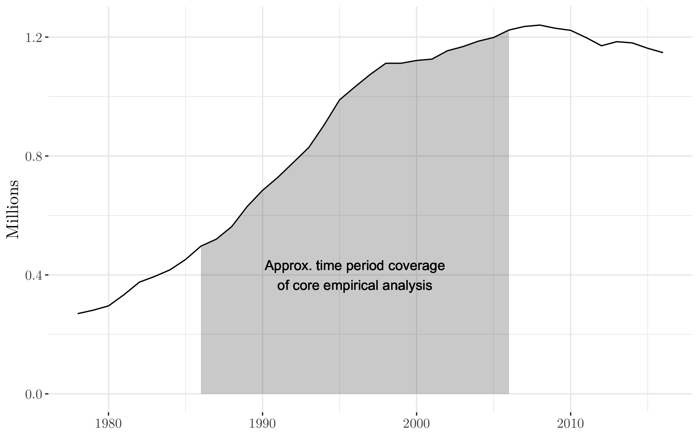
Figure 1: United States Prison Population (State & Federal)

Note: Source of the prison population data is the United States Department of Justice Office of Justice Programs (Bureau of Justice Statistics). Core empirical analysis in this study includes entire term of all district attorneys listed in the issues of the National Directory of Prosecuting Attorneys found between 1987 and 2005. Consequently, the coverage years indicated in the graph are approximate values with only slight variation by district, because DAs have different start/end years for their 4-year terms based on the respective district.

National Corrections Reporting Program (NCRP)—This represents the primary source for sentencing data used in this study. NCRP collects offender-level data on admissions and releases from state and federal prison. The NCRP records include offender-level information such as: BJS offense category, state offense category, total sentence, race, gender, age, prior felony status, county, and state where sentence imposed. The analysis includes the full universe of records on prison admissions. Sentenced months corresponds with the longest length of time as stated by the court that the offender could be required to serve for all offenses of which they have been convicted.

Table 1: Summary Statistics of State Prison Sentencing Outcomes

	Mean	Median	Standard Deviation
Admissions/1000 Population
All Offenses	1.68	1.21	2.83
Violent Offenses	0.42	0.31	0.70
Drug Offenses	0.50	0.30	1.21
Property Offenses	0.63	0.48	0.87
Sentenced Months/1000 Population
All Offenses	141.73	99.32	215.02
Violent Offenses	65.61	42.86	115.62
Drug Offenses	37.03	18.81	74.35
Property Offenses	40.40	27.75	52.37

Notes: Data cover roughly 1986–2006 and 42,500 county-years.

4.2 Election Data

Election data was compiled from various sources. Election results of district attorneys were compiled from states, counties, and other sources (see dataset indicated in [21]). The Database on Ideology, Money in Politics, and Elections (DIME) contains over 130 million political contributions made by individuals and organizations for local, state, and federal elections between 1979 and 2014; it also includes information on candidates and committees for state and federal elections [11].

5 Empirical Strategy

5.1 Dynamic Difference-in-Differences Model (for Election Effects on Criminal Sentencing Outcomes)

In this paper, I adopt a quasi-experimental research design to estimate the effects of election cycles on the decision-making of district attorneys. County-level variation in the timing of district attorney elections resulted in substantial variation across counties that I exploit using a series of dynamic difference-in-differences specifications:

$$Y_{cst}=\gamma_{s}+\lambda_{t}+\sum_{k=-T}^{T-1}\beta_{k}\mathbbm{1}\{R_{ct}=k\}+\Gamma_{cst}+\varepsilon_{cst}$$ (2)

The dependent variable $Y_{cst}$ corresponds to one of two outcome variables—(1) admissions/ capita or (2) months sentenced/capita—evaluated for county $c$ in state $s$ in time period $t$. Time period $t$ is evaluated in either years or in months. On the right-hand-side, let $R_{ct}=t-E_{c}$ denote the “relative time”—the number of periods relative to the nearest election period for the district attorney in county $c$ in time period $t$. $T$ equals half the length of a district attorney’s term in office. $\gamma_{s}$ are state fixed effects, $\lambda_{t}$ are year fixed effects, and $\Gamma_{cst}$ is a vector of controls. The standard errors are corrected for correlation across district attorneys and over time in a given county by clustering at the district level.

The coefficients of interest are $\beta_{k\neq\text{normalized year}}$, which are the effects on outcomes in years that do not correspond to the normalized year. I indicate in each section below which election cycle time period I use to normalize results. For example, if I normalize such that $\beta_{-2}=0$, that would mean for a district attorney serving in county $c$ in time period $t$, the $\beta_{k\neq-2}$ coefficients measure the sentencing outcomes relative to the sentencing outcomes two time periods prior to the election period. In the Results section, I express these coefficients in log points, which is a rough approximation of the percentage point difference in sentencing outcomes in non-election years compared to outcomes in election years.

I first estimate these models using the NCRP data for which I also have data on the corresponding prosecutor from the National Directory of Prosecuting Attorneys. The NCRP data contain offender-level information, such as BJS offense category, total sentence, county, and state where sentence imposed. The sample for each year consists of all states that reported data who had four-year election cycles.

As always, the identifying assumption for difference-in-differences estimation strategies is the parallel trends assumption, which in this case is that any differential change in outcomes in district attorney election years is the result of the district attorney election. Perhaps the greatest challenge to this identifying assumption is that even if there were no district attorney elections in the particular election year, there might still be elections for other offices related to law enforcement (e.g., sheriff elections). These alternative elections may have direct (and indirect) effects on sentencing outcomes. I address this issue by re-running the analysis only including election cycles in which the district attorney elections are not synchronous with those of other offices. As mentioned later in Section 6.4.2, the effects largely remain.

5.2 Static Difference-in-Differences Model (for Mechanisms & Election Effects Heterogeneity)

To explore potential mechanisms behind the results from Equation 2, I exploit a series of static difference-in-differences specifications:

$$Y_{cst}=\gamma_{s}+\lambda_{t}+\beta D_{ct}+\Gamma_{cst}+\varepsilon_{cst}$$ (3)

The dependent variable $Y_{cst}$ corresponds to one of two outcome variables—(1) admissions/capita or (2) months sentenced/capita—evaluated for county $c$ in state $s$ in year $t$. On the right-hand-side, let $D_{ct}$ denote the treatment, which is an indicator variable denoting whether county $c$ is in an election year in year $t$. $\gamma_{s}$ are state fixed effects, $\lambda_{t}$ are year fixed effects, and $\Gamma_{cst}$ is a vector of controls. The standard errors are corrected for correlation across district attorneys and over time in a given county by clustering at the district level.

The coefficient of interest is $\beta$, which is the effect on outcomes from being in an election year.

6 Results

6.1 Impact of Election Cycles on Criminal Sentencing Outcomes

Figure 2 graphically depicts estimates of the effects of election cycles on two separate criminal sentencing outcomes across all offenses: (1) admissions per 1000 population; and (2) total sentenced months per 1000 population. These graphs follow the regression specification from Equation 2. All estimates are calculated relative to the election year value, which is normalized to 0. Hence, if the estimates at time $t=-1$ and $t=1$ are both negative, this can be interpreted as the election year (when $t=0$) having a relatively higher magnitude of the corresponding criminal justice outcome compared with the year prior and the year after. All estimates are in log points. A log point estimate of $a$ approximates a $(100\cdot a)\%$ effect when the magnitude of $a$ is small. Vertical lines mark standard errors.

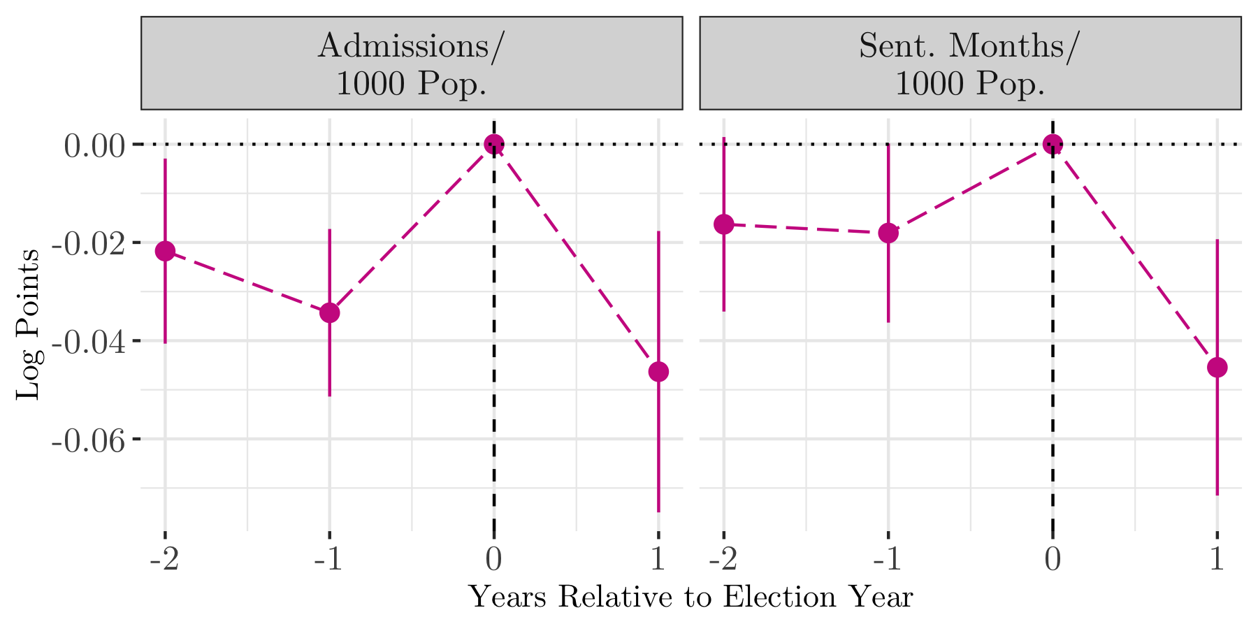
Figure 2: Criminal Sentencing Outcomes,
Relative to District Attorney Election Year

Notes: Graph depicts dynamic difference-in-differences model estimates using Equation 2 (weighted to adjust for differences in sampling probabilities across districts and across time). Estimates are at the county level by year. The standard errors are corrected for correlation across district attorneys and over time in a given county by clustering at the district level. Estimates include state- and year- fixed effects. Vertical lines mark two standard errors. Estimates calculated relative to the election year value, which is normalized to 0. Corresponding regression table is in the Appendix.

The graphs provide evidence that election years have effects on the admissions rate per 1000 population and the sentenced months per 1000 population. The estimated effects of an election year on the admissions rate are statistically significant and positive, compared to all non-election years. The estimated effects of an election year on sentenced months per 1000 population are also positive for all non-election years, with the effect being statistically significant for the year immediately following the election year.

Figure 3 again illustrates estimates of the effects of election cycles on criminal sentencing outcomes using regression specification Equation 2, this time by criminal offense subcategory. This analysis provides evidence that similar effects persist across offense subcategories, with the impact on sentenced months relative to adjacent years being less pronounced for drug offenses compared to property and violent offenses. Not only is the effect of election years on admissions rate positive and statistically significant across most non-election years for each crime subcategory, but also the magnitude of this impact on admissions rate appears similar across offense subcategories.

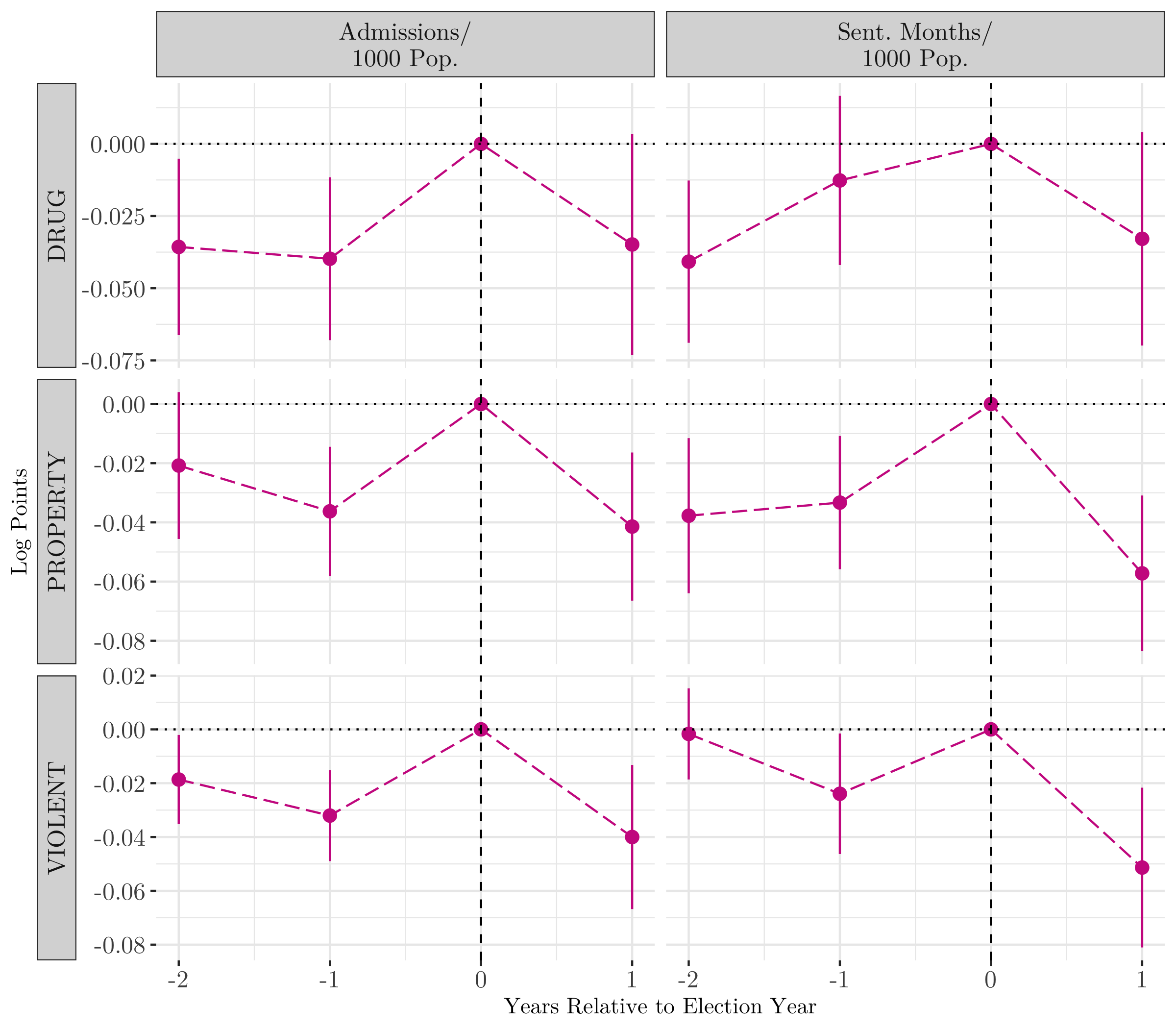
Figure 3: Criminal Sentencing Outcomes,
Relative to District Attorney Election Year – Offense Subcategories

Notes: Graph depicts dynamic difference-in-differences model estimates using Equation 2 (population weighted to adjust for differences in sampling probabilities across districts and across time). Estimates are at the county level by year. The standard errors are corrected for correlation across district attorneys and over time in a given county by clustering at the district level. Estimates include state- and year- fixed effects. Vertical lines mark two standard errors. Estimates calculated relative to the election year value, which is normalized to 0. Corresponding regression table is in the Appendix.

Heterogeneity of election year effects across crime categories could be affected by various potential factors, including differences in political risk from lenient behavior, as well as varying levels of discretionary power DAs possess for different crime categories. First, there could be greater political risk associated with being lenient on certain crime categories than for others (e.g., consider the political incentives for being harsh on a high-profile murder vs. being harsh on low-level drug possession). In addition, mandatory minimum sentencing is more prominent for certain crime categories than others, which could impact the discretion prosecutors have in plea bargaining negotiations. This in turn might be a factor in explaining heterogeneity in election year effects across crime categories.

6.2 Monthly Sentencing Outcomes

This subsection presents another analysis of Equation 2, this time with the time period observed in months and all coefficients measured relative to the months omitted from the graph (the months which are furthest from the election year).

Figure 4 illustrates the estimates for total months sentenced for property offenses during roughly the one year period before an election year, during the election year itself, and during the one year period after the election year. A corresponding regression table is in the Appendix. The plot shows perhaps the most clear consistent upward trend in the outcome variable from about 15 months prior to the election through the middle of the election year. Since individual criminal cases are generally unrelated to each other, it is reasonable to interpret each dot as a collection of independent observations. Thus, the fact that the dots are close together and increasing in the period immediately preceding a general election suggests that there is in fact an increasing trend occurring during this time period.

One can clearly see that all the estimates during the election year are greater than zero, which is not the case for the time periods before and after the election year—and is also not true for the time period omitted from the graph, since that period has been normalized to zero. Also, one can see that the estimates immediately following the election year have the greatest concentration of estimates below zero (followed by the period preceding the election year), which is consistent with the prediction from the theoretical model that the sentencing intensity district attorneys exert increases in the election year. Political incentives and their impact on prosecution may be lowest just after an election concludes.

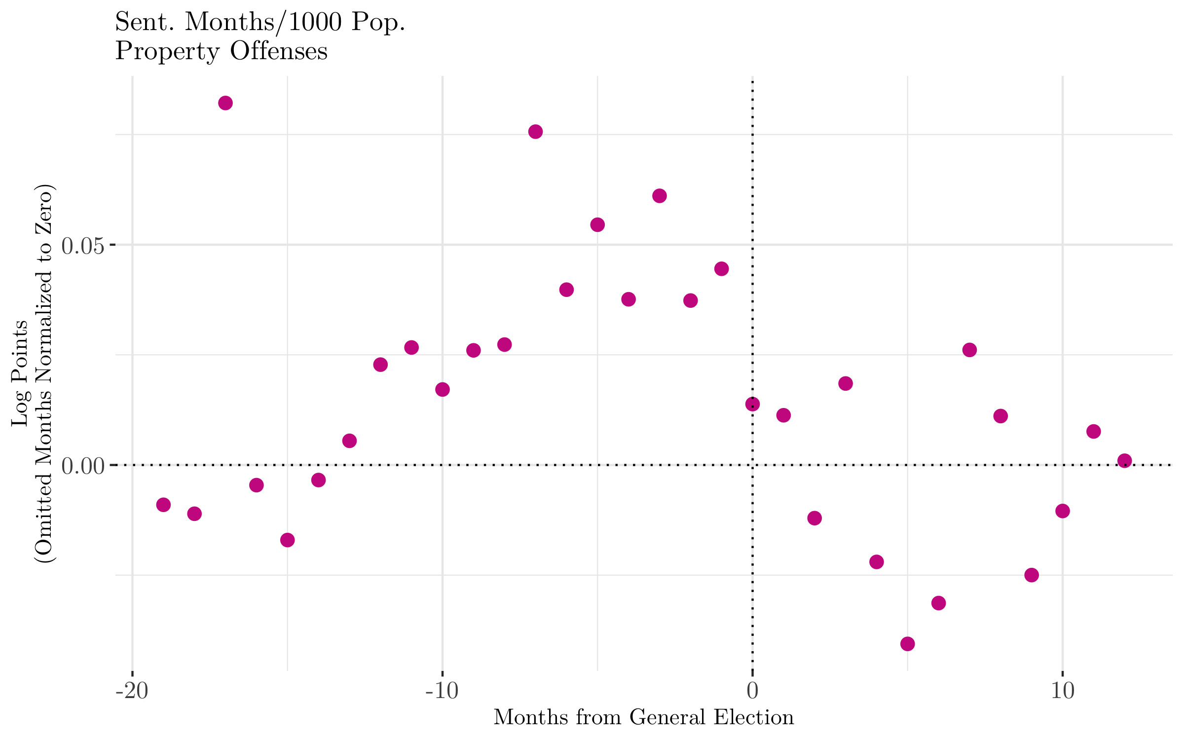
Figure 4: Monthly Total Sentenced Months in Election Cycle (Property Offenses)

Notes: Graph depicts dynamic difference-in-differences model estimates using Equation 2 (population weighted to adjust for differences in sampling probabilities across districts and across time). Estimates are at the county level by month. Estimates include state- and year-month- fixed effects. Vertical lines mark two standard errors. Estimates calculated relative to omitted months in election cycle, which are all normalized to 0. Corresponding regression table is in Appendix.

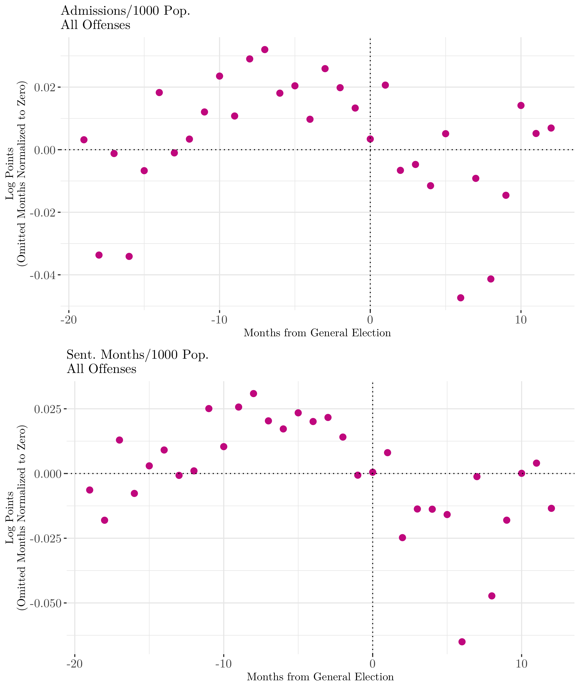
Figure 5: Monthly Criminal Sentencing Outcomes in Election Cycle

Notes: Graph depicts dynamic difference-in-differences model estimates using Equation 2 (population weighted to adjust for differences in sampling probabilities across districts and across time). Estimates are at the county level by month. Estimates include state- and year-month- fixed effects. Vertical lines mark two standard errors. Estimates calculated relative to omitted months in election cycle, which are all normalized to 0. Corresponding regression table is in Appendix.

Figure 5 illustrates a similar plot as Figure 4, except looking at the average across all offense categories. Again, the corresponding regression tables are in the Appendix. It is apparent that the sentencing outcomes for both admissions per capita and sentenced months per capita is higher during the election year period than during the time periods before and after, which is consistent with the property offense plot from Figure 4. Furthermore, one can see that just about all the estimates during the election year are greater than zero, which is not the case for either of the two other time periods included in the graph. Also, one can see that the estimates immediately preceding the election year are more frequently lower than the election year period, which is again consistent with the theoretical model from Equation 1. Specifically, this plot provides evidence that the estimates for both admissions per capita and sentenced months per capita increase over the election cycle on average. In other words, the period immediately following the election has the lowest estimates (with a negative mean), then the estimates increase in the second year after the election (which has been normalized to zero), then they increase again in the period immediately preceding the election year, and then increase again during the election year itself. This is consistent with the perspective that DAs may respond to political incentives associated with the election cycle.

One slight puzzle is that there seems to be a single lagging positive estimate that extends into the last month of the election year (at $t=1$) for the admissions rate plot. This slight outlier is not present in the months sentenced plot nor in the property offenses plot from Figure 4, suggesting it might be due to an alternative offense subcategory. One potential explanation for this estimate is that there might be an administrative time lag between when district attorneys are making relevant charging and plea bargaining decisions and the date the ultimate admission occurs and is consequently captured in the dataset. In short, there may be short-term spillover of election year effects into the period immediately following the election.

6.3 Magnitude of Election Year Effects

To interpret the magnitude of the election year effects, I adopt a similar methodology for signal variance as described in various papers [12, see, e.g.,]. Signal variance ($\gamma^{2}$) allows one to interpret the magnitude of election year effects in units of standard deviations (based on the underlying distribution of district attorney sentencing behavior).

Here I describe the basic steps and intuition I employ to calculate $\gamma^{2}$. First, I estimate the mean sentencing behavior for each prosecutor. I do so by computing district attorney fixed effects for the underlying outcome variables. Second, I compute an estimate of how much variation there is across district attorneys in the outcome variable (within state). I accomplish this by regressing state fixed effects on the set of district attorney fixed effects, then calculate the Mean Squared Error from this regression. It is important to realize that this measure of variation across district attorneys within state is partly driven by noise (e.g., from sampling variation). Consequently, as a third step, I subtract the amount of variation coming from the noise. To do so, I subtract the average standard error of the prosecutor fixed effects squared.

In short, I estimate $\gamma^{2}$ by subtracting the average sampling variance across district attorneys from the variance of the residuals obtained by regressing state fixed effects on district attorney fixed effects. This yields $\gamma_{admissions}^{2}=0.0323$ for the admissions rate per capita and $\gamma_{months}^{2}=0.0364$ for the total months sentenced per capita. I then take the election year estimates calculated from the static difference-in-differences specification in Equation 3 and compare it to the (square root) signal variance. Doing so tells us that, on average, the election year effects on admissions are akin to moving 0.85 standard deviations along the distribution of prosecutor sentencing behavior within state. This means that with respect to the admissions rate, being in an election year is akin to going from the 50th percentile of district attorney sentencing intensity to the 80th percentile. The election year effects on months sentenced are akin to moving 0.62 standard deviations along the distribution of prosecutor sentencing behavior, on average. This means that with respect to the months sentenced, being in an election year is akin to going from the 50th percentile of district attorney sentencing intensity to the 73rd percentile.

6.4 Robustness Checks

6.4.1 Alternative Weighting for Two-Way Fixed Effects (TWFE) Estimator

Linear regressions with time period and group fixed effects estimate weighted sums of the average treatment effect (ATE). A recent series of papers has found that some of the weights in this weighted sum may be negative in settings with variation in treatment timing across units of observation [49, 15]. Due to the potential impact of negative weights, the calculated regression coefficients could be negative even if all ATEs were in fact positive. Given this potential problem in the calculation of regression coefficients in the two-way fixed effects model, here I construct an alternative estimator introduced by [49]. The authors explain that this alternative estimation approach is robust to treatment effects heterogeneity.

The goal is to estimate a weighted average of the cohort average treatment effects on the treated ($CATT_{e,k}$); this average represents the average treatment effect $k$ periods from an election year for the cohort of all counties with election years at time $e$. We want to estimate $CATT_{e,k}$ with more reasonable weights than would occur if the original two-way fixed effects specification had negative weights (i.e., we estimate the effects with weights that are non-negative and sum to one). Due to the main empirical specification employed in this paper (described earlier as Equation 2), the following expression is used:

$$v_{g}=\frac{1}{\lvert g\rvert}\sum_{k\in g}\sum_{e}CATT_{e,k}\Pr\{E_{c}=e\}$$ (4)

where $v_{g}$ is the weighted average of $CATT_{e,k}$, $k$ is the “relative time”—the number of periods relative to the nearest election year. $g$ is the collection of all periods included in the regression expression. $e$ is the time of treatment for observations belonging to the same cohort. $E_{c}$ is the time of the treatment (i.e., an election year). I estimate the weights $\Pr\{E_{c}=e\}$ by sample shares of each cohort in the relevant periods $k\in g$.

Per [49], I estimate $CATT_{e,k}$ using a linear two-way fixed effects specification that interacts indicators for the relative year with indicators of the corresponding cohort:

$$Y_{cst}=\gamma_{s}+\lambda_{t}+\sum_{e}\sum_{k\notin 0}\delta_{e,k}\left(\mathbbm{1}\{E_{c}=e\}\cdot D^{k}_{c,t}\right)+\varepsilon_{cst}$$ (5)

The coefficient estimator $\hat{\delta}_{e,k}$ from Equation 5 is a difference-in-difference estimator for $CATT_{e,k}$. $D^{k}_{c,t}$ are indicator variables corresponding to being $k$ years from an election year in county $c$ at year $t$. Similar to Equation 2, I exclude interactions with $D^{0}_{c,t}$, so that the estimated coefficients are relative to the sentencing outcomes in the election year. Plugging $\hat{\delta}_{e,k}$ from Equation 5 into $CATT_{e,k}$ from Equation 4 allows us to calculate $v_{g}$ for various sentencing outcomes. In normalizing the election year estimate to zero, negative values for $v_{g}$ correspond with a positive relative effect from being in an election year compared to non-election periods.

Table 2: Coefficients for Alternative TWFE Weighting

	$CATT$ ($v_{g}$) (log points)	Bootstrap Standard Error
Admissions / 1000 Pop.
All Offenses	-0.045	0.0117
Violent Offenses	-0.032	0.0107
Property Offenses	-0.020	0.0119
Drug Offenses	-0.076	0.0146
Sentenced Months / 1000 Pop.
All Offenses	-0.037	0.0116
Violent Offenses	-0.012	0.0105
Property Offenses	-0.015	0.0109
Drug Offenses	-0.072	0.0162

Table 2 illustrates that the re-weighted coefficients for the ATE ($v_{g}$) remain negative for both admissions per capita and sentenced months per capita, with standard errors estimated via a bootstrap sampling procedure. Furthermore, these coefficients are negative for each crime subcategory (i.e., violent, property, and drug), and consistently statistically significant for the All Offenses and Drug Offenses categories. The sign of these coefficients—and the average magnitude across all offenses—are consistent with the findings from the original specification Equation 2, providing evidence that the original specification does in fact show the correct sign of the underlying average treatment effect.

6.4.2 Parallel Trends Assumption

The key identifying assumption for the difference-in-differences empirical approach used throughout this Section is parallel trends. In other words, the identifying assumption is that—in the absence of the treatment of the district attorney being in an election year—there would be no discernible impact on criminal sentencing outcomes (i.e., per capita admissions rate and per capita months sentenced).

[30, 27] find that municipal police forces tend to vary over local and state electoral cycles. Yet even if higher police forces did coincide with mayoral election years—and such mayoral elections did in turn coincide with district attorney elections—evidence suggests this would not violate the parallel trends assumption. [36] states that in the case of the COPS program, increasing the number of police officers did not appear to increase arrest rates, suggesting potential offenders were deterred from committing crimes by the larger police presence. This deterrent effect is consistent with [26], which finds that arrest rates appeared to reduce the frequency of many different types of crimes, not just ones likely to be committed by the [incapacitated] person, thereby suggesting a deterrent effect from greater police activity.

Particularly because evidence suggests larger (election year) police forces may primarily impact crime through greater deterrence, then if election effects on sentencing were in fact caused by increases in municipal police forces, one would not expect an increase in the admissions rate or total sentenced months during the election period. To the contrary, one would expect the election period estimates to have the opposite sign: the deterrent effect would lead to lower admissions and lower total sentenced months. As such, it is difficult to ascribe the DA election year increases in admissions and months sentenced to changes in police presence. In addition to this descriptive evidence, I provide further evidence later in this Section that the parallel trends assumption holds with regard to the potential confounding factor of increased police presence. I do so via an empirical analysis.

Another potential challenge to the parallel trends assumption are judicial elections. Yet as was described earlier in this paper, in recent times plea bargaining has been the mode of conviction for over 95 percent of convicted felons in counties, meaning individual sentences were strongly influenced by negotiations with the district attorney and not by the outcomes of judge or jury trials. Although judges have the power to not approve a plea bargain, they rarely do so [51]. In addition, the transition from indeterminate sentencing to determinate sentencing in the late 1970s caused state legislatures to pass laws that constrained the discretion of judges as well as parole boards [34]. Sentencing policies, such as mandatory minimums, presumptive sentencing ranges, truth-in-sentencing laws, and two- and three-strike laws, provide determinate guidelines judges must follow in sentencing decisions, greatly limiting the amount they can affect criminal sentencing outcomes [37, 34]. In contrast, policies analogous to sentencing guidelines for judges do not exist for district attorneys. DAs have unreviewable discretion on whether to bring charges, and can strategically select the collection of charges for a criminal suspect that incorporates sentencing guidelines, based on how severe or lenient they wish to be. Thus, district attorneys have much control over admissions—through choosing whether or not to charge an individual with a crime—and sentence length, through choosing which collection of charges to bring against a criminal suspect. In contrast, the channel through which judicial elections would meaningfully increase the extensive margin—the number of individuals actually admitted to state prisons—is less convincing. These facts provide evidence that the parallel trends assumption holds with regards to the potential confounding factor of judicial elections.

A third challenge to the parallel trends assumption is sheriff elections. The scope of the sheriff role varies across states and counties. The sheriff is most often an elected officer, and in some counties where urban areas have their own police departments, a sheriff may be restricted to civil procedure enforcement duties; in other counties, the sheriff may serve as the principal police force with jurisdiction over all the county’s municipalities. In the latter case, the sheriff may be responsible for enforcing criminal law. The earlier facts I cite regarding the deterrent impact of police presence similarly provides evidence the parallel trends assumption holds for sheriff elections, I also test empirically this assumption by analyzing the district attorney election year effects when the district attorney elections do not coincide with the sheriff elections.

The parallel trends assumption empirical analysis relies on data from [6, 50] for mayors and sheriffs, respectively. The [6] data consists of 9,131 mayoral elections, and includes data from several different sources on elections between 1950 and 2014 in cities of all sizes. I merge the city election data with the corresponding county, and use the gap between two consecutive election years to determine the historical incidence of elections for a particular municipality. This allows me to perform the same alternative two-way fixed effects estimator I performed in the previous subsection—illustrated in Figure 6 below—this time removing county-years in which the district attorney election year was synchronous with a local mayoral election. For this analysis, I only include counties in which one can identify whether or not there was a synchronous mayoral election; counties without corresponding mayoral election data were not included in the analysis. I perform a similar analysis with the sheriff election data from [50], which includes over 3,200 partisan sheriff elections.

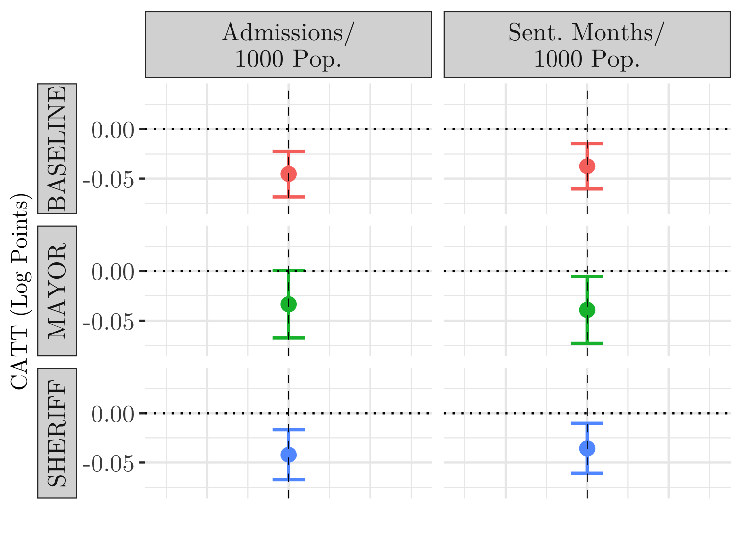
Figure 6: Criminal Sentencing Outcomes, Relative to District Attorney Election Year – Non-Synchronicity with Other Elected Office (Alternative TWFE Estimator)

Notes: Mayor and sheriff non-synchronous analysis omits areas where no data found to determine synchronicity with district attorney election cycle. Baseline analysis includes all district attorney election cycles. Estimates tabulated by county and by year, and calculated in accordance with alternative two-way fixed effects estimator [49, see]. Observations weighted by county population. Vertical lines mark two standard errors. Estimates calculated relative to the district attorney election year value, which is normalized to 0.

Figure 6 illustrates that after removing county-years in which the district attorney election was synchronous with the mayoral election and sheriff election, the direction and magnitude of the election year effects remain—even under the alternative two-way fixed effects estimator. This provides further (empirical) evidence that the parallel trends assumption holds.

6.4.3 Other Robustness Checks

Further robustness checks were also performed. For example, the findings in this study are robust to specifications in which the set of controls—white share of the population and income—are not included. The findings are also robust to county (instead of state) fixed effects. Also, the shape of the curve depicting the relationship between the election cycle and criminal sentencing outcomes is preserved under a log transformation—log(1+x)—of the data; the utility of this transformation is that it prevents zeros from being omitted from the regression analysis. See the Appendix for graphs of the primary election cycle analyses with log transformations.

7 Mechanisms

The results thus far document that the admissions rate per capita and the rate of total months sentenced per capita increase in the lead up to general elections during an era of rising incarceration (roughly 1986 to 2006). This time period overlaps with the greatest expansion in incarceration levels in the history of the United States. In this section, I perform additional analysis to shed light on various mechanisms underlying the findings.

7.1 Evidence that DA Election Effects Not Explained by Changes in Arrest Rates or Crime Rates

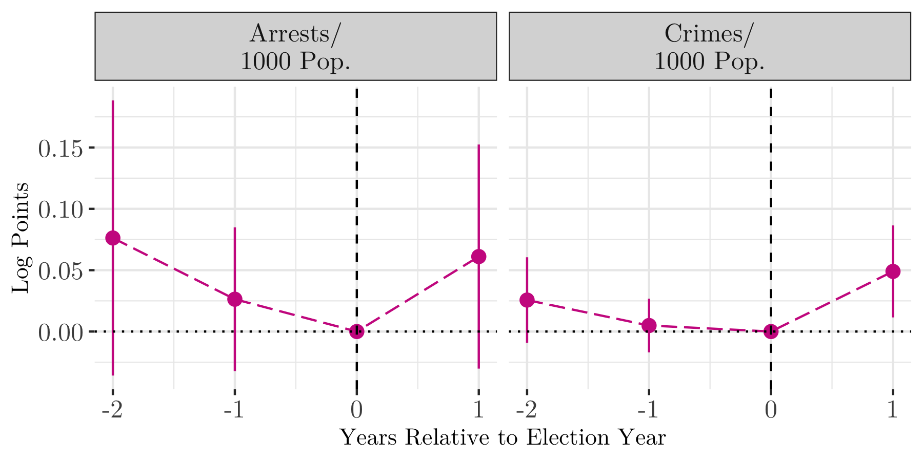
Figure 7: Arrest & Crime Rates,
Relative to District Attorney Election Year

Notes: Graph depicts dynamic difference-in-differences model estimates using Equation 2 (weighted to adjust for differences in sampling probabilities across districts and across time). Estimates are at the county level by year. The standard errors are corrected for correlation across district attorneys and over time in a given county by clustering at the district level. Estimates include state- and year- fixed effects. Vertical lines mark two standard errors. Estimates calculated relative to the election year value, which is normalized to 0. Corresponding regression table is in the Appendix.

Figure 7 graphically depicts estimates of the effects of DA election cycles on per capita arrest rates and per capita crime rates, via the regression specification from Equation 2. The plot shows there is no statistically significant election year effects on the volume of arrests and crimes (unlike the core election effects on criminal sentencing outcomes). If anything, the election year volume of arrests and crimes are slightly lower than in non-election years. Hence, Figure 7 does not support the notion that the main election effects on criminal sentencing outcomes can be explained by changes in the volume of arrests or crimes around elections. This finding is consistent with the earlier parallel trends analysis: even under an assumption that mayoral and sheriff elections were synchronous with the DA elections (and in which there might consequently be political pressure to increase police presence and impact the volume of arrests), it would not explain the election effects found in this study. Furthermore, this analysis of arrests and crimes suggests the DA election effects are similarly not attributable to changes in criminal behavior; this evidence suggests that potential criminal activity does not spike in or near DA election years. Taken together, the evidence is consistent with the perspective that the district attorney election year effects on criminal sentencing outcomes are attributable to district attorneys themselves and not attributable to changes in criminal behavior, police presence, or the behavior of other elected officials.

7.2 DA Election Effects Depend on County Political Ideology More than DA Ideology; Effects Larger in Contested Elections

Figure 8 shows the association of county, prosecutor, and election traits with DA election year effects on criminal sentencing outcomes. Whereas the political ideology of the district has a statistically significant association with the election year effects, evidence suggests the political ideology of the district attorneys themselves do not. Across both outcomes, the association between being a conservative DA and the election year effects is weakly positive. Counties that were Republican in the most recent Presidential election had statistically significant and positive association with election year effects for both outcome variables. Counties that were Republican on more than 6 out of 10 elections from 1980 to 2016 had a lower positive association with election year effects, an association that was only positive for the admissions rate. These findings suggest that it is the most recent (Republican) political dynamics that most influence election year effects on sentencing outcomes, a conclusion which in turn is consistent with the perspective (and with the theoretical model from Equation 1) that political incentives from reelection concerns impact district attorney behavior.

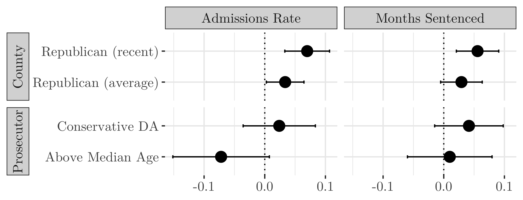
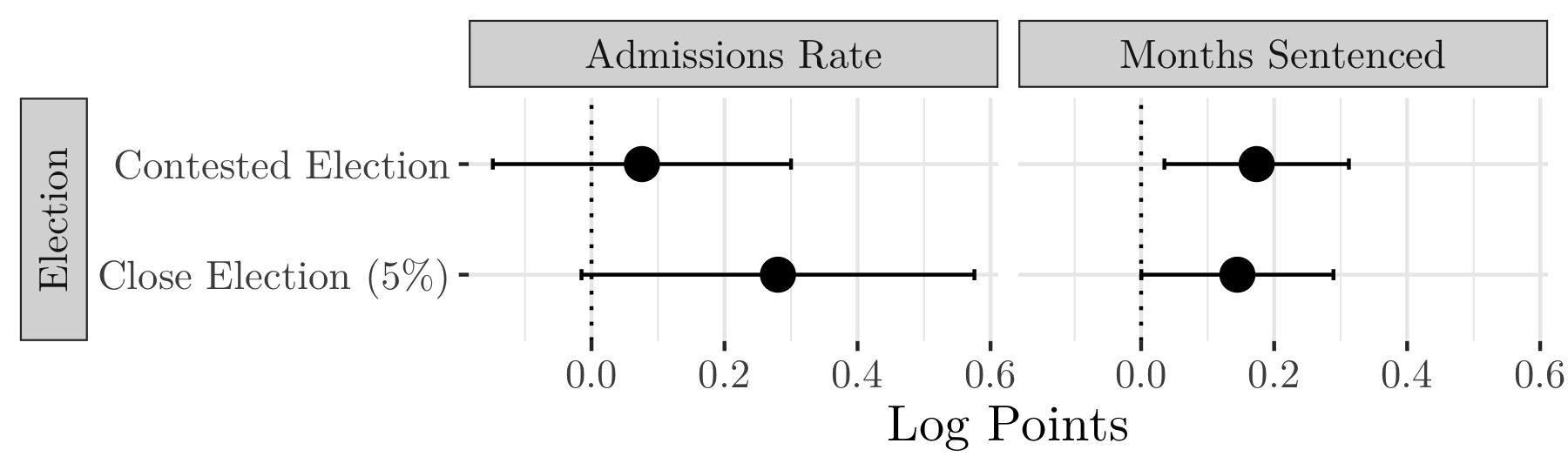
Figure 8: Association of County, Prosecutor, & Election Traits with Election Year Effects

Notes: Graph depicts a static difference-in-differences model (population weighted to adjust for differences in sampling probabilities across districts and across time). Estimates are at the county level by year. The standard errors are corrected for correlation across district attorneys and over time in a given county by clustering at the district level. Estimates include state- and year- fixed effects. Horizontal lines mark two standard errors. “Republican (recent)” corresponds with counties that voted for a Republican Presidential candidate in the most recent election. “Republican (average)” corresponds with counties that voted for a Republican Presidential Candidate in more than 6 out of 10 elections from 1980 to 2016. District attorney and election characteristics analysis based on subset of overall counties where data was found.

The salience of reelection concerns is reinforced by the bottom plot in Figure 8. The plot demonstrates that being in a contested or close election is associated with greater election year effects (though only the effect on the months sentenced is statistically significant). This election analysis is based on a subset of the total county-years, reflecting those county-years in which corresponding election data were successfully compiled (from state and county data). This election data covers approximately 4,000 district attorney general elections from the 1980s onward.

7.3 DA Election Effects Concentrated in South Central U.S.

To begin our spatial analysis of the election year effects, let us return to the monthly sentencing outcome analysis from Section 6.2. The objective is to estimate the magnitude of the election period effect given the relative time from an upcoming election. To capture potential non-linearities, I regress sentencing outcomes on a transformation of the relative time from an election $\mathit{f}(R_{ct})$:

$$Y_{cst}=\gamma_{s}+\lambda_{t}+\beta\times\mathit{f}(R_{ct})+\varepsilon_{cst}$$ (6)

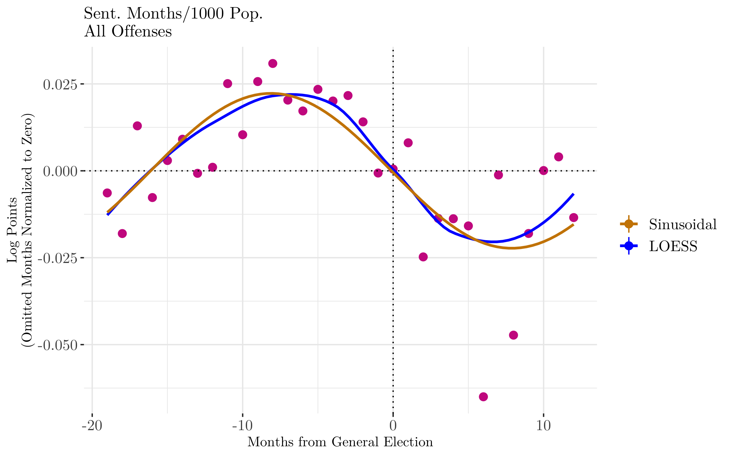
Figure 9: Parameterizing Sentencing Outcomes

Notes: Graph depicts a dynamic difference-in-differences model (population weighted to adjust for differences in sampling probabilities across districts and across time). Estimates are at the county level by year. Estimates include state- and year- fixed effects. Plot includes non-parametric LOESS best-fit line and parametric sinusoidal model.

where $\mathit{f}(R_{ct})$ is estimated using a LOESS regression. Intuitively, I first fit a LOESS regression to the non-parametric conditional expectation functions plotted previously in Figure 5 to find a transformation of relative time from an election—$\mathit{f}(R_{ct})$—that renders the relationship between $Y_{cst}$ and $\mathit{f}(R_{ct})$ linear. Through observation of Figure 9 below, an appropriate transformation appears to be sinusoidal. Hence, one approach I use in this section is to estimate partial effects on the amplitude $A$ from the following specification evaluated with time $t$ in years (since differences in the $A$ parameter roughly correspond to differences in the magnitude of election year effects):

$$Y_{cst}=\gamma_{s}+\lambda_{t}+A\cdot\sin(2\pi R_{ct}/4+\phi)+\varepsilon_{cst}$$ (7)

A second approach I use is the static difference-in-differences model from Equation 3, evaluating the $\beta$ parameter. Based on these two approaches, I examine how election effects vary by geographic region. Figure 10 shows election year effects by region for both outcome variables, with the maps on the lefthand side shaded according to partial effects from the static difference-in-differences model (Equation 3). The righthand side of the figure shows the corresponding partial effects based on both the static diff-in-diff model and the sinusoidal model (Equation 7), evaluated with the time period in years. One can see that the largest election year effects on admissions rate is consistently in the South Central region of the U.S. (east and west). Furthermore, these effects significantly differ from zero for both modeling approaches. New England and the East North Central regions have negative election year effects, with the estimate from the sinusoidal model being significant and largely negative. The election year effects in many other geographic regions are not statistically different than zero.

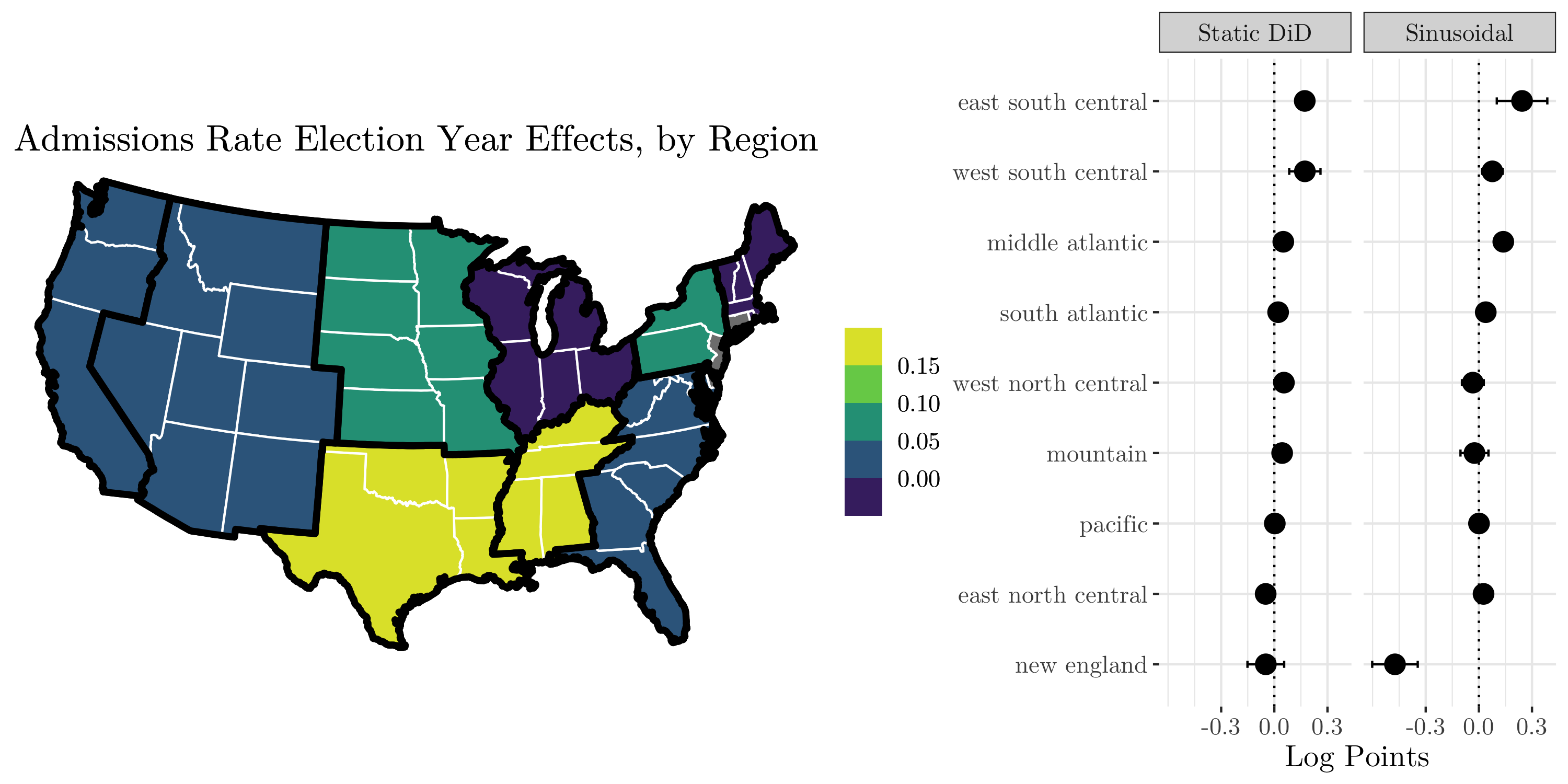
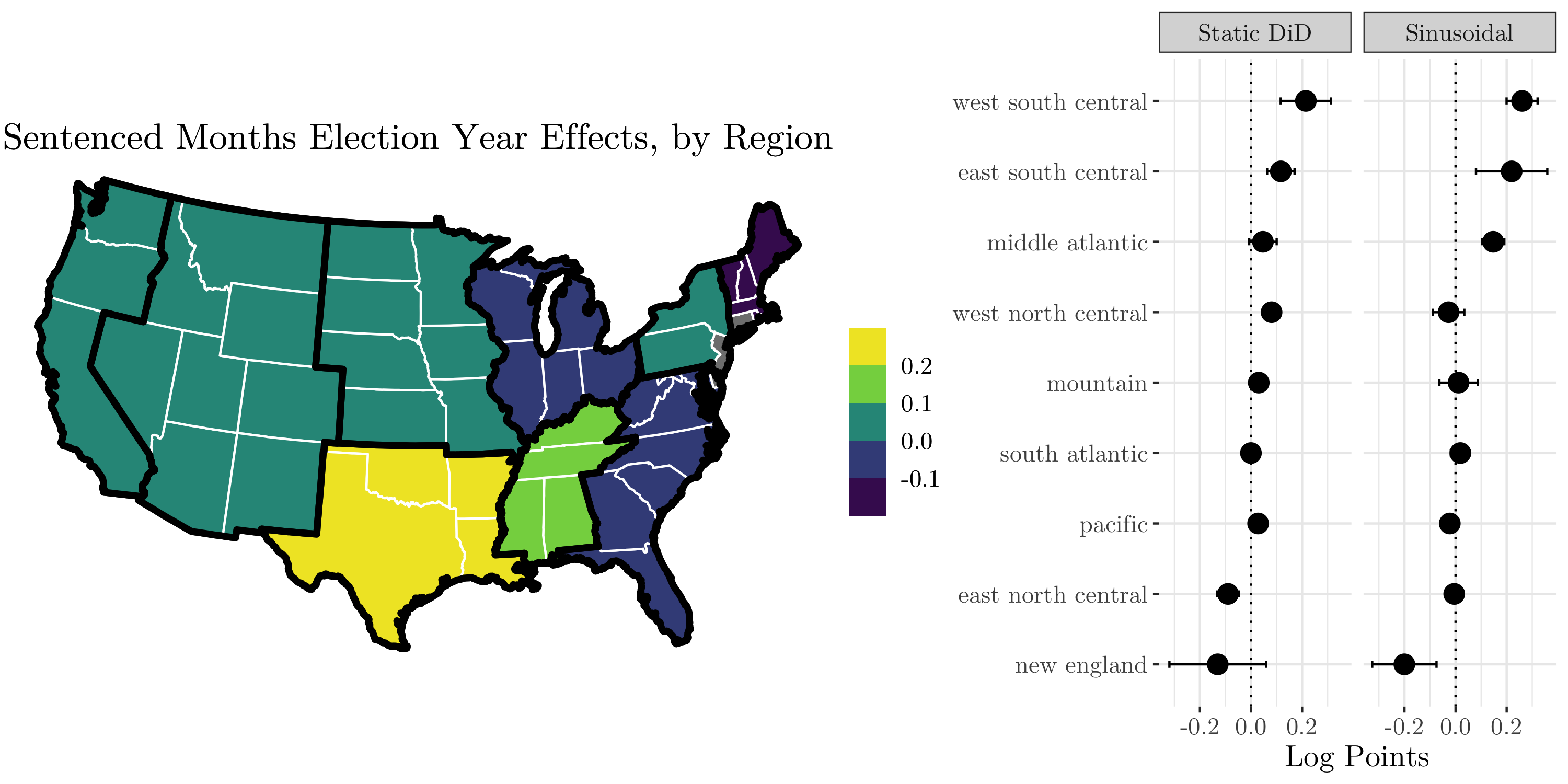
Figure 10: Election Year Effects By Region

Notes: Map shading depicts a static difference-in-differences model (population weighted to adjust for differences in sampling probabilities across districts and across time). Estimates are at the county level by year. The standard errors are corrected for correlation across district attorneys and over time in a given county by clustering at the district level. Estimates include state- and year- fixed effects. Horizontal lines mark two standard errors. Heterogeneity across regions calculated via a static difference-in-difference model and a sinusoidal model, respectively.

The plot for the months sentenced outcome show similar results, with the largest estimated election year effects for the South Central region (east and west). Again, New England and East North Central—which is the region that includes Chicago—are negative, with each region’s estimate significant in just one of the two models.

7.4 DA Election Effects Declined in Era of Rising Incarceration, Coinciding with Softening Public Opinion on Punishment

A key question—which our data allows us to consider—is how election year effects have evolved over time. This question is particularly relevant in light of several recent developments: the emergence of the term “mass incarceration” to characterize the prison trends since the 1980s; the emergence of “progressive prosecutors” who explicitly run on a platform counter to being “tough-on-crime,” and the recent bipartisan efforts toward criminal justice reform. These developments, among others, suggest that the political incentives that many prosecutors face may be different than those in the 1980s and 1990s.

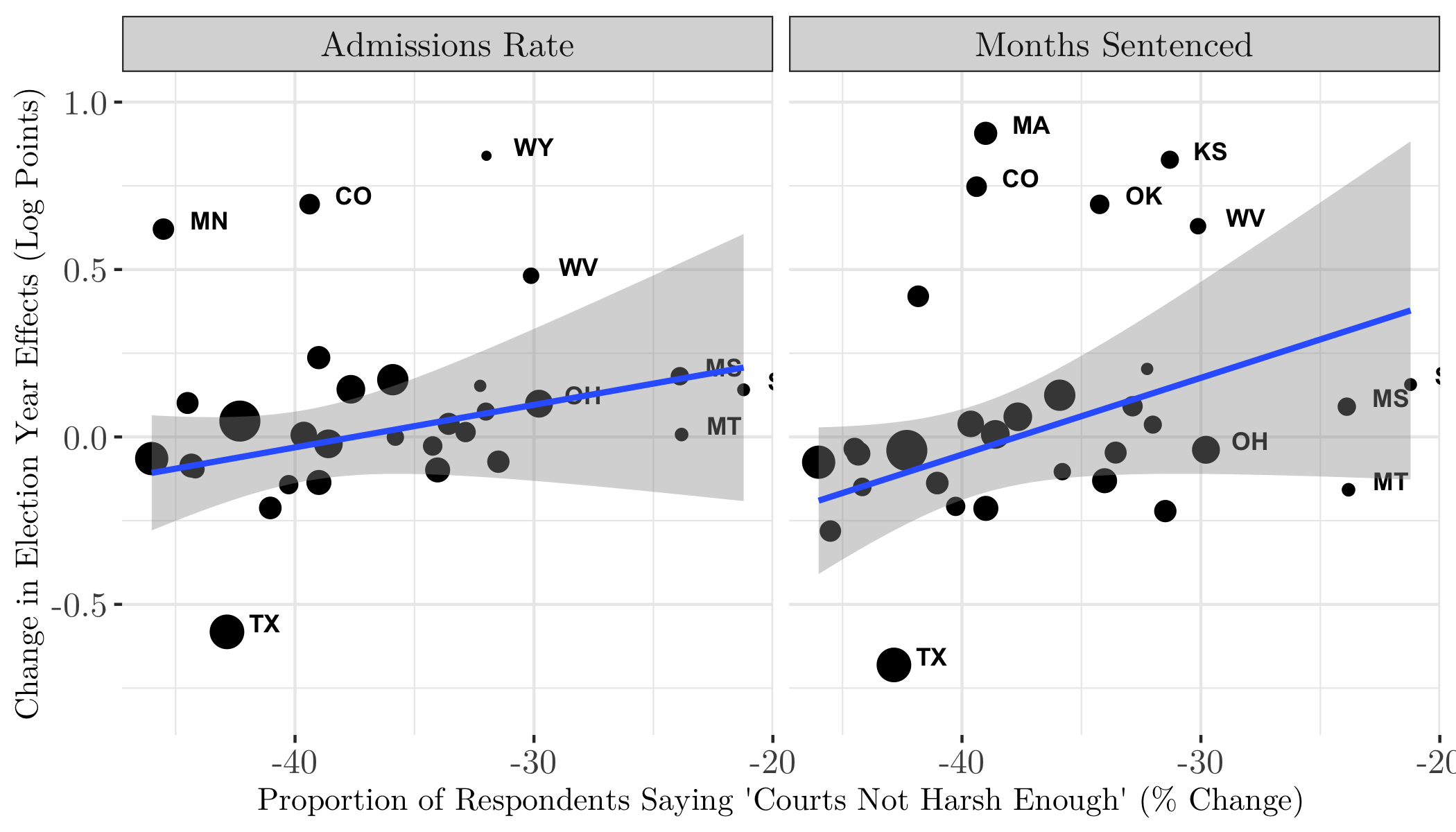
Figure 11: Change in Election Year Effects, by State (Pre-2000 Period to Post-2000 Period)

Notes: Change in election year effects calculated using a static difference-in-differences model (population weighted to adjust for differences in sampling probabilities across districts and across time). Estimates include year- fixed effects. Size of dots corresponds with mean state population between 1983 and 2016. Proportion of respondents saying “Courts Not Harsh Enough” taken from the General Social Survey (GSS) [46]. The GSS is a nationally-representative survey (and not so at a sub-national or state-level of analysis).

In Figure 11, I compare the relationship between changes in public opinion and changes in election year effects—comparing the 16 years before 2000 with the 16 years after 2000. The y-axis is the change in election year effects between these two periods. The x-axis is a proxy for the change in public opinion—namely, the percent change in respondents from the General Social Survey (a longitudinal survey administered yearly since the 1970s) who say courts are not harsh enough. So in short, the further left you are on the x-axis, the more lenient the corresponding public opinion has become over time. Each dot represents a state, with the size corresponding to population. Of note, across all states, the public has increasingly viewed courts as too harsh. The relationship between the level of change in public opinion and the level of change in election year effects is weakly positive for the admissions rate. The relationship is more positive for months sentenced. These findings provide suggestive evidence that the election year effects are related to public opinion toward criminal punishment, with states who have had the greatest decline in respondents viewing the courts as “not harsh enough” also having the greatest decline in election year effects.

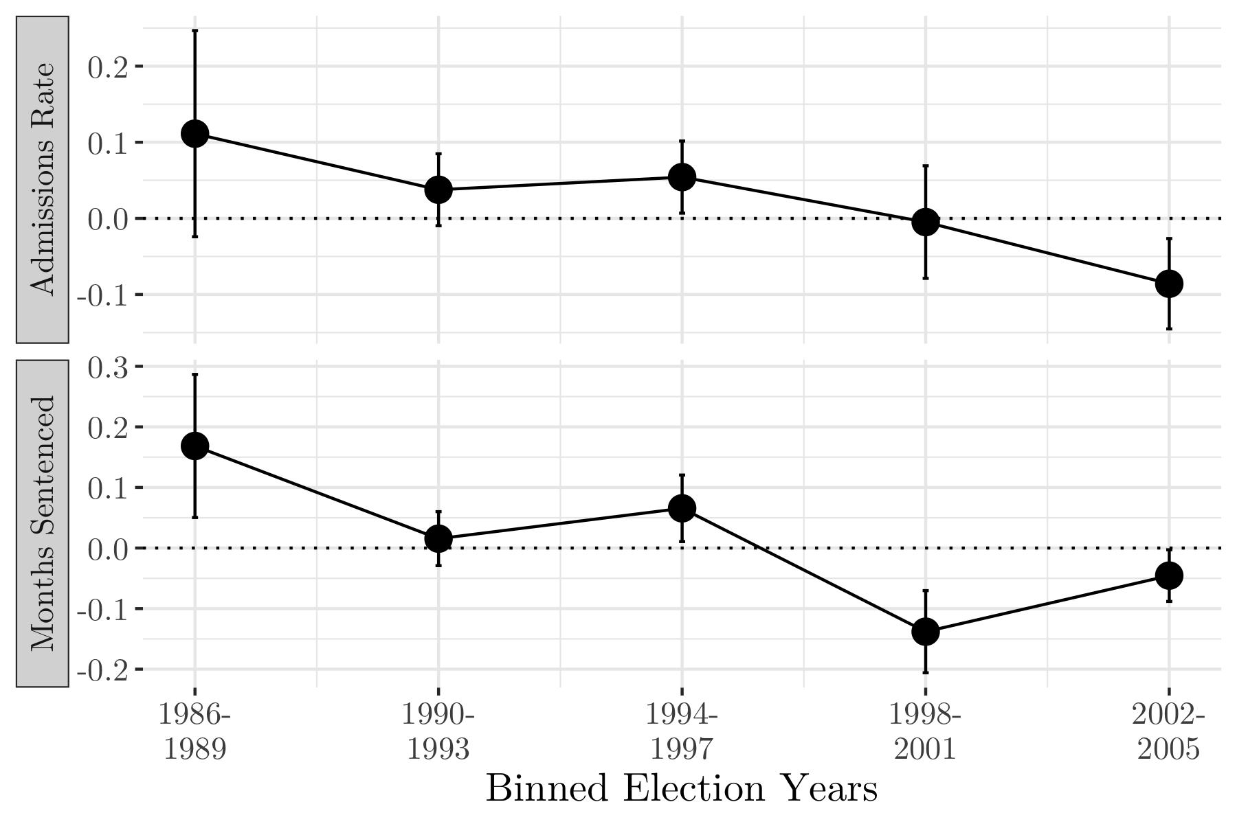
Figure 12: Election Year Effects Over Time vs.
Public Opinion Over Time

Notes: Graph depicts a static difference-in-differences model (population weighted to adjust for differences in sampling probabilities across districts and across time). Estimates are at the county level by year. The standard errors are corrected for correlation across district attorneys and over time in a given county by clustering at the district level. Estimates include state- and year- fixed effects. Horizontal lines mark two standard errors.

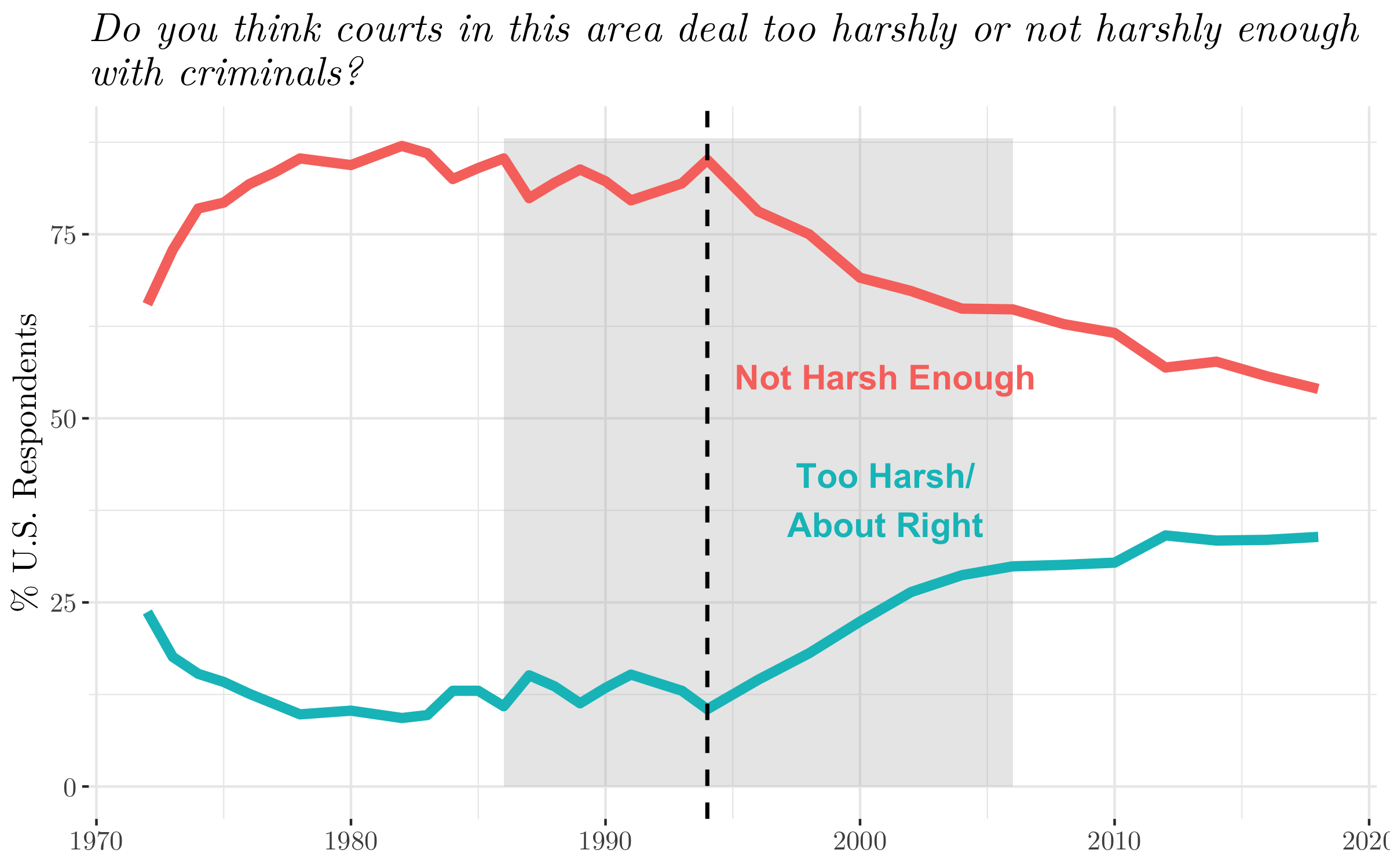
Notes: Source is the GSS [46]. “Don’t Know” responses excluded. Vertical dashed line corresponds with the year 1994. Shaded region corresponds with the approximate coverage of core empirical analysis illustrated in Figure 1 and explained in Section 4 (an era of rising incarceration).

The change in election year effects over time in the top plot of Figure 12 is also consistent with the view that an evolution in public sentiment over time impacted DA behavior. In the 1980s and 1990s, anecdotally there was a lot more discussion about—and perhaps perceived benefit from—being a politician who was viewed as being “tough-on-crime.” This was the period of the spike in crack-related drug convictions, the passing of the 1994 crime bill, and the establishment of minimum sentencing laws around the country. The GSS shows that in fact the vast majority of the population believed courts were not harsh enough. The bottom plot of Figure 12 shows that only after 1994 did this fraction of the population begin to decline. In contrast, those who believed courts were too harsh or about right have become a growing share of the population since 1994. In short, public sentiment toward punishment has been shifting over the last 25 years or so. This shift coincides with lower election year effects over time, and plausibly impacted the political incentives faced by district attorneys.

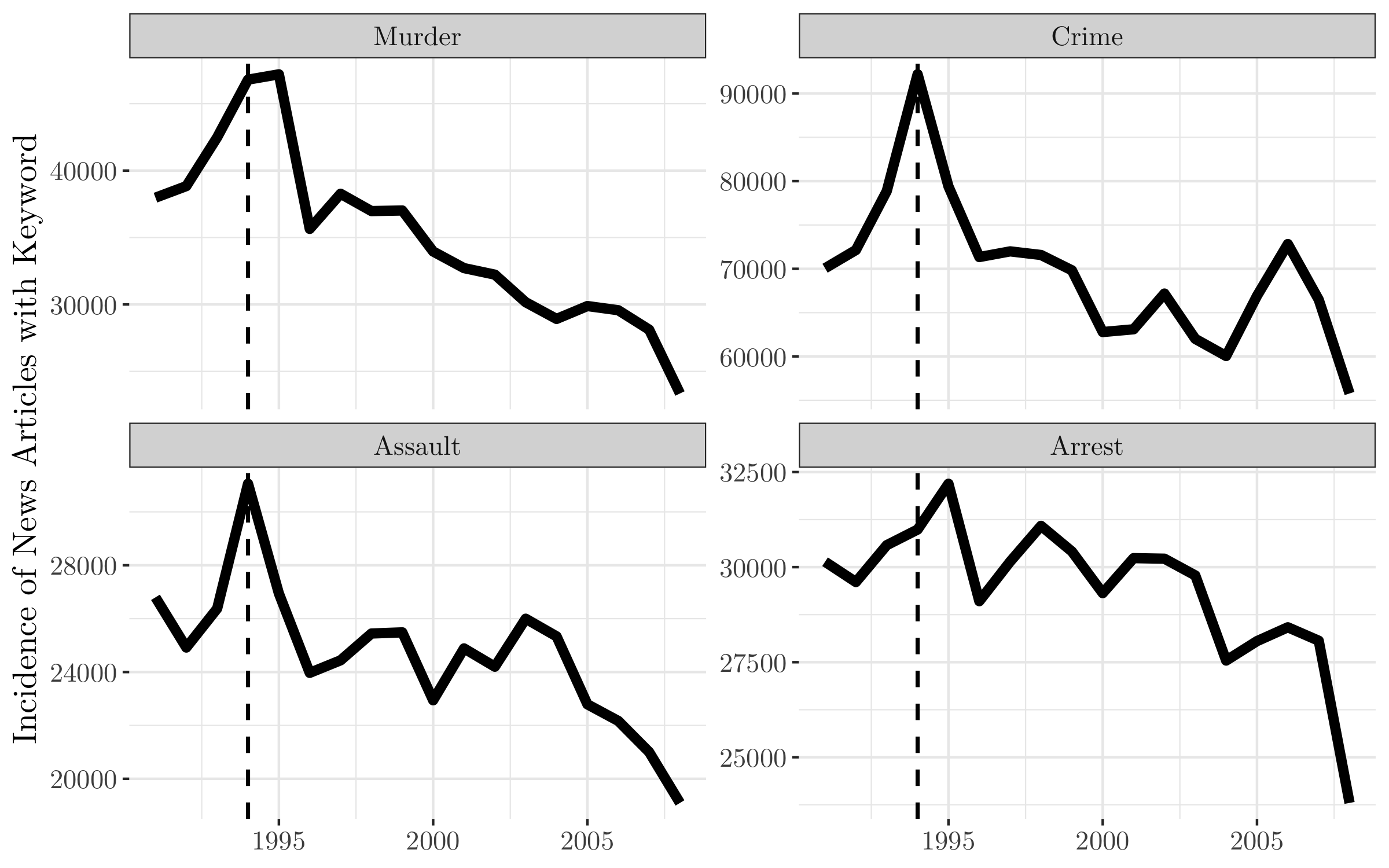
Figure 13: Salience of Leading Local Newspaper Articles with Crime-Related Language, 1991–2008

Notes: Article counts taken from one of the top three newspapers in each respective state. Searches performed via Factiva, Nexisuni, Hollis, or WestlawNext. Given data availability, analysis begins from 1991 onward and includes the following states: Alaska, Arizona, California, Colorado, Connecticut, District of Columbia, Florida, Georgia, Kansas, Kentucky, Louisiana, Maryland, Massachusetts, Minnesota, Missouri, Nevada, New Hampshire, New York, North Carolina, Ohio, Oklahoma, Oregon, South Carolina, Texas, Utah, Virginia, Washington, and Wisconsin. Newspapers used in analysis can be found in Appendix B.2.

There is plausibly a nexus between (1) changes in public opinion over time, and (2) changes in the salience of criminal activity over time. In other words, the public may adopt a more lenient stance toward criminal punishment in periods in which crime is less prominent. The guiding hypothesis is clear: the salience of crime is plausibly more impactful on public sentiment—and in turn the political incentives district attorneys face—than the actual crime rate, since salience more proximately influences voter perceptions than the crime levels themselves. Under this hypothesis—and based on the public sentiment trends described in Figure 12—one would expect that the softening of public opinion toward punishment would coincide with (and potentially be caused by) a declining salience of criminal activity in the public eye. The GSS figure at the bottom of Figure 12 illustrates a clear shift in the public opinion trend line after the year 1994. Now compare that shift in trends with Figure 13. Figure 13 shows the incidence of top local newspaper articles that include various crime-related keywords; in short, it can be viewed as proxy for the salience of crime in the public eye. Strikingly, again we see a clear break in the trend line around the year 1994, after which the incidence of articles mentioning various crime-related language begins to decline. This general decline occurs for articles that include the word “murder,” “crime,” “assault,” and “arrest.” Yet, the downward trend is most apparent for articles that contain the word “murder.” Murders may possess the greatest nexus with public sentiments toward criminal punishment (given the extreme severity and grotesqueness of the offense). Hence, the sharp decline in local newspaper coverage of murder (and other crime-related terms) after 1994 is consistent with the perspective that the softening of public sentiment toward punishment is in response to the declining salience of criminal activity in the public eye.

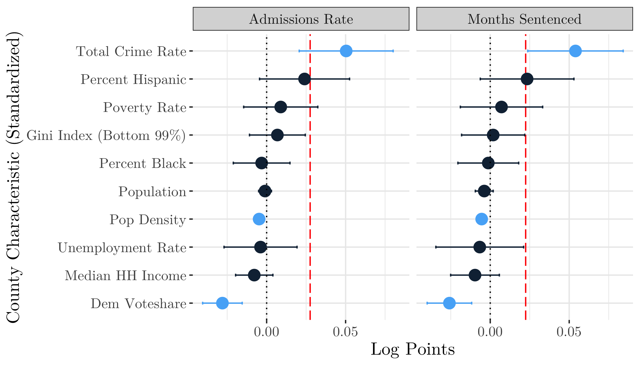
Figure 14: Association of County Characteristics with Election Year Effects

Notes: Source of county characteristics data is Opportunity Insights (www.opportunityinsights.org). Estimates reflect a static difference-in-differences model (population weighted to adjust for differences in sampling probabilities across districts and across time). Estimates are at the county level by year. The standard errors are corrected for correlation across district attorneys and over time in a given county by clustering at the district level. Estimates include state- and year- fixed effects. County characteristics are standardized, so estimates reflect change in election year effect from a one standard deviation change in corresponding characteristic. Horizontal lines mark two standard errors. Vertical red dashed line represents the main election year effect. Dem Voteshare is vote share in previous Presidential election going to Democratic candidate. All county characteristics calculated from the mean value between 1986–2006.

To deepen our understanding of potential mechanisms explaining this relationship between public sentiment and election year effects, I calculate the association between various standardized county characteristics and election year effects. Figure 14 shows the result of this analysis, based on the static difference-in-differences model (Equation 3). The red vertical line represents the main effect—the election year effect in the absence of interactions with county characteristics. The figure illustrates that a one standard deviation increase in the total crime rate is associated with a five log points increase in election year effects for both outcome variables. The magnitude and significance of total crime rate (compared with other county characteristics) is consistent with the perspective that election year effects are responsive to public opinion. Greater crime rates may impact public opinion, perhaps by galvanizing the public against those convicted of crimes, which in turn might increase the political pressure prosecutors might face in being harsher on crime.

Figure 14 also shows that democratic voteshare, which measures the fraction of votes going to the Democratic Presidential candidate in the prior election, is the second most influential county characteristic in the plot. It is negatively associated with the election year effects and it is statistically significant for both outcomes. Again, we see that the political ideology of the district is associated with election year effects, which is consistent with the notion that it is public opinion, or the public’s general sentiment toward crime, that is creating political incentives for district attorneys.

Proposition 2

As the difference decreases between the marginal returns to reelection probability from sentencing intensity ($\frac{\partial P(s(e_{1}),s(e_{2}))}{\partial s(e_{2})}-\frac{\partial P(s(e_{1}),s(e_{2}))}{\partial s(e_{1})}$), the difference also decreases between the sentencing intensity between periods ($s(e_{2})-s(e_{1})$).

The proof for Proposition 2 is included in the Appendix. Recall that Proposition 1 from the theoretical model in Equation 1 holds that more prosecuting effort will be expended in the election year than in the period preceding it ($e_{2}>e_{1}$), yielding greater sentencing intensity during election periods ($s(e_{2})>s(e_{1})$). This is because: (1) sentencing intensity is positively correlated with the probability of reelection ($\frac{\partial P(s(e_{1}),s(e_{2}))}{\partial s(e_{1})},\frac{\partial P(s(e_{1}),s(e_{2}))}{\partial s(e_{2})}>0$), combined with (2) the election period sentencing intensity $s(e_{2})$ has comparatively larger marginal returns to reelection probability ($\frac{\partial P(s(e_{1}),s(e_{2}))}{\partial s(e_{2})}>\frac{\partial P(s(e_{1}),s(e_{2}))}{\partial s(e_{1})}$). Historical trends on public sentiment toward crime help elucidate how the relationship between sentencing intensity and reelection prospects may evolve over time. The political science literature generally views elections as a means of accountability for public officials. Hence, as was consistent in the 1980s and 1990s, the public perception that courts were not harsh enough suggests reelection probability would clearly be positively correlated with sentencing intensity. Yet, as public sentiment toward crime softened from 1994 onward, the correlation between sentencing intensity and reelection probability plausibly softened as well. Formally, this could mean the difference between $\frac{\partial P(s(e_{1}),s(e_{2}))}{\partial s(e_{2})}$ and $\frac{\partial P(s(e_{1}),s(e_{2}))}{\partial s(e_{1})}$ would decrease, as sentencing intensity in both time periods would increasingly be providing less information to voters on district attorney job performance; in short, severity is becoming an increasingly less-useful performance metric since voters increasingly view courts as already too harsh. As a result, Proposition 2 predicts the election year effects on sentencing intensity would flatten out (i.e., the difference $s(e_{2})$ minus $s(e_{1})$ would narrow). This prediction is borne out through the empirical analysis provided earlier in this Section.

8 Discussion

Violent offenses plausibly have the greatest likelihood of catalyzing public backlash if punishments are deemed too lenient. Such crimes bear more risk of becoming high-profile, as they represent the most serious offenses and arguably elicit the greatest fear of a lack of public safety. An extension of this study could disaggregate violent offenses, to identify whether the most severe ones (e.g., murder and rape) have the greatest election year effects.

If sentencing outcomes were solely determined by the DA’s personal philosophy toward punishment, one might not expect there to be much cyclicality in the severity of outcomes. One would simply expect the districts with DAs having harsher theories of punishment to have consistently more severe sentences. Instead, we see greater election year effects in Republican counties, which is consistent with the perspective that DA behavior incorporates political incentives, such as voters’ perceived preferences for harshness. Future analysis might explore “progressive prosecutors”—based on the finding that political incentives for sentencing intensity differ markedly between liberal and conservative districts, this may translate to different behaviors in the run-up to elections for various DA offices. Other legal scholars have already touted the potential for progressive prosecutors to help reform the system [21]. One would expect not only that areas with progressive prosecutors would have lower overall sentences, but based on this study one would also expect there to be no election year effects—or perhaps election year effects that are less harsh—for districts where progressive prosecutors are politically viable.

There are at least two obvious interpretations of the election year effects this study finds: (1) that the election year severity of sentencing is too high, based on prevailing theories of justice; (2) that the election year severity of sentencing is adequate, and instead the severity for non-election years is too low. Given the fact that the United States has the highest incarceration rate in the world, the second interpretation may be less plausible than the first one. Under the first interpretation, politics may have encouraged overly severe sentencing outcomes. In short, under this first interpretation, the argument for reducing political incentives of district attorneys becomes more salient—particularly when the public’s desire for harshness diverges from what may be considered “fair” or socially optimal.

Accordingly, the findings relate to broader legal debates on the efficacy of “democratizing” the criminal justice system [22, see, e.g.,]. On one side of the argument are those who attribute many problems with the criminal justice system to an ill-informed (or particularly vengeful) American public; this side tends to call for the justice system to be more greatly influenced by professionals and experts. On the other side of the argument are those who attribute the problems with the justice system to bureaucratic attitudes and other institutional/structural problems. This side tends to call for more control of the system from local communities, with greater responsiveness to the lay public. For those skeptical of democratizing the criminal justice system, a potential corrective response to the election year effects could be to transition the DA selection process from an electoral system to appointment. Several states already operate under this model, such as Delaware, New Jersey, Alaska, and Connecticut.

Some legal scholars, however, question the political feasibility of accomplishing this shift [23, 52, see, e.g.,]. For those who support increased democratization of the criminal justice system, appropriate corrective responses to the election year effects found in this paper are less clear. As scholars like [38] argue, even if criminal justice actors were made more accountable to local communities, it remains unclear whether the lay public in the local communities most afflicted by crime would necessarily encourage more leniency. There could be unintended consequences, with more democratization potentially yielding political incentives to increase severity of sentences. Similarly, proposals to increase the competitiveness of DA elections [21, see, e.g.,] may exacerbate the impact of election cycles on sentencing outcomes. Ultimately, the myriad consequences of further democratization in the DA selection process may remain an empirical question—one that I leave for future research.

9 Conclusion

This paper only evaluates the short-term cyclical impact of being in an election year on sentencing outcomes. It does not capture potential longer-term political considerations that might impact how district attorneys approach their work at all periods in the election cycle. This means the full impact of political incentives on the criminal justice system and mass incarceration may be larger than what is found in this paper alone. So much work on criminal justice reform to date has focused on improvements to the system itself and to the laws that govern it. If the political incentives of those entrusted to administer justice are shaped by public sentiment regarding criminal punishment, then this paper highlights that focusing on “hearts and minds”—on shifting public opinion toward punishment independent of shifts to laws or to the structure of the criminal justice system itself—may prove not only beneficial but also instrumental in improving sentencing outcomes and stemming mass incarceration.

Appendix A

Proof of Proposition 1. The first-order conditions for the problems in Equation 1 are:

$$e_{1}:-2e_{1}+1+\delta^{2}\cdot P_{s(e_{1})}(s(e_{1}),s(e_{2}))\cdot s^{\prime}(e_{1})\cdot V=0$$

$$e_{2}:-2e_{2}+1+\delta\cdot P_{s(e_{2})}(s(e_{1}),s(e_{2}))\cdot s^{\prime}(e_{2})\cdot V=0$$

The assumptions made on prosecuting effort, sentencing intensity, and reelection probability functions guarantee that (a) $e_{1},e_{2}>0$; (b) $P_{s(e_{2})}(\cdot),P_{s(e_{1})}(\cdot)>0$; (c) $P_{s(e_{2})}(\cdot)>P_{s(e_{1})}(\cdot)$; and (d) $s^{\prime}(e_{1})=s^{\prime}(e_{2})$ in all scenarios. Combining first-order conditions yields the expression: $e_{1}=e_{2}-\frac{\delta}{2}(P_{s(e_{2})}(\cdot)s^{\prime}(e_{2})-\delta P_{s(e_{1})}(\cdot)s^{\prime}(e_{1}))V$. Since $\delta\in(0,1]$, the expression implies $e_{2}>e_{1}$. Since $s^{\prime}(\cdot)>0$ by assumption, this implies $s(e_{2})>s(e_{1})$.   

Proof of Proposition 2. The first-order conditions for the problems in Equation 1 are:

$$e_{1}:-2e_{1}+1+\delta^{2}\cdot P_{s(e_{1})}(s(e_{1}),s(e_{2}))\cdot s^{\prime}(e_{1})\cdot V=0$$

$$e_{2}:-2e_{2}+1+\delta\cdot P_{s(e_{2})}(s(e_{1}),s(e_{2}))\cdot s^{\prime}(e_{2})\cdot V=0$$

Let $k=P_{s(e_{2})}(\cdot)-P_{s(e_{1})}(\cdot)$. Substituting for $P_{s(e_{1})}(s(e_{1}),s(e_{2}))$, combining first-order conditions, and simplifying yields:

$$k=P_{s(e_{2})}(\cdot)-\frac{P_{s(e_{2})}(\cdot)}{\delta}+\frac{2}{\delta^{2}s^{\prime}(e_{1})V}(e_{2}-e_{1})$$

The assumptions guarantee that $\delta>0$, $s^{\prime}(\cdot)>0$, and $V>0$. Hence, on inspection one can see that $k$ is positively correlated with the difference $e_{2}-e_{1}$. Since $s^{\prime}(\cdot)>0$, in equilibrium $k$ is also positively correlated with the difference $s(e_{2})-s(e_{1})$.   

Appendix B

Table B.1: Number of States Included in National Corrections Reporting Program, by Year

Year	# States Reporting
1983	26
1984	42
1985	38
1986	50
1987	50
1988	50
1989	50
1990	50
1991	50
1992	46
1993	46
1994	44
1995	45
1996	44
1997	45
1998	45
1999	48
2000	49
2001	48
2002	50
2003	48
2004	48
2005	48
2006	48
2007	46
2008	48
2009	48
2010	47
2011	47
2012	48
2013	46
2014	47
2015	43
2016	43

Table B.2: Leading Local Newspaper Included in Crime Keyword Analysis (Figure 13)

State	Newspaper	City
Alaska	Anchorage Daily News	Anchorage
Arizona	The Arizona Daily Star	Tucson
California	Los Angeles Daily News	San Diego
Colorado	The Denver Post	Denver
Connecticut	Hartford Courant	New Haven
N/A	The Washington Post	District of Columbia
Florida	Tampa Bay Times	Jacksonville
Georgia	The Atlanta Journal-Constitution	Atlanta
Kansas	The Wichita Eagle	Wichita
Kentucky	Lexington Herald-Leader	Lexington
Louisiana	New Orleans Times Picayune	Baton Rouge
Maryland	Baltimore Sun	Baltimore
Massachusetts	The Boston Globe	Boston
Minnesota	Star Tribune	Minneapolis
Missouri	St. Louis Post Dispatch	St. Louis
Nevada	Las Vegas Review-Journal	Las Vegas
New Hampshire	New Hampshire Union Leader	Manchester
New York	The New York Times	New York
North Carolina	The Charlotte Observer	Charlotte
Ohio	The Columbus Dispatch	Columbus
Oklahoma	The Oklahoman	Oklahoma City
Oregon	The Oregonian	Portland
South Carolina	The State	Charleston
Texas	Houston Chronicle	Houston
Utah	The Salt Lake Tribune	Salt Lake City
Virginia	The Virginian-Pilot	Virginia Beach
Washington	The Seattle Times	Seattle
Wisconsin	Milwaukee Journal Sentinel	Milwaukee

Appendix C

Table C.1: Sentencing Outcomes, by Years from Election Year (All Offenses)

	Dependent variable (in Log Points)
	Admissions/1000 Pop.	Months/1000 Pop.
	(1)	(2)
-1	$-$0.034∗∗∗ (0.009)	$-$0.018∗ (0.009)
1	$-$0.046∗∗∗ (0.015)	$-$0.045∗∗∗ (0.013)
-2	$-$0.022∗∗ (0.010)	$-$0.016∗ (0.009)
Observations	41,950	39,620
	∗p$<$0.1; ∗∗p$<$0.05; ∗∗∗p$<$0.01

Notes: Table depicts dynamic difference-in-differences model estimates using Equation 2 (population weighted to adjust for differences in sampling probabilities across districts and across time). Estimates are at the county level by year. The standard errors are corrected for correlation across district attorneys and over time in a given county by clustering at the district level. Estimates include state- and year-month- fixed effects. Estimates calculated relative to election year, which is normalized to 0.

Table C.2: Sentencing Outcomes, by Years from Election Year (Violent Offenses)

	Dependent variable (in Log Points)
	Admissions/1000 Pop.	Months/1000 Pop.
	(1)	(2)
-1	$-$0.032∗∗∗ (0.009)	$-$0.024∗∗ (0.011)
1	$-$0.040∗∗∗ (0.014)	$-$0.051∗∗∗ (0.015)
-2	$-$0.019∗∗ (0.008)	$-$0.002 (0.009)
county_population	0.00000∗∗ (0.000)	0.00000∗∗∗ (0.000)
Observations	38,314	36,174
	∗p$<$0.1; ∗∗p$<$0.05; ∗∗∗p$<$0.01

Notes: Table depicts dynamic difference-in-differences model estimates using Equation 2 (population weighted to adjust for differences in sampling probabilities across districts and across time). Estimates are at the county level by year. The standard errors are corrected for correlation across district attorneys and over time in a given county by clustering at the district level. Estimates include state- and year-month- fixed effects. Estimates calculated relative to election year, which is normalized to 0.

Table C.3: Sentencing Outcomes, by Years from Election Year (Property Offenses)

	Dependent variable (in Log Points)
	Admissions/1000 Pop.	Months/1000 Pop.
	(1)	(2)
-1	$-$0.036∗∗∗ (0.011)	$-$0.033∗∗∗ (0.011)
1	$-$0.041∗∗∗ (0.013)	$-$0.057∗∗∗ (0.013)
-2	$-$0.021 (0.013)	$-$0.038∗∗∗ (0.013)
county_population	0.000 (0.000)	0.000 (0.000)
Observations	38,734	36,296
	∗p$<$0.1; ∗∗p$<$0.05; ∗∗∗p$<$0.01

Notes: Table depicts dynamic difference-in-differences model estimates using Equation 2 (population weighted to adjust for differences in sampling probabilities across districts and across time). Estimates are at the county level by year. The standard errors are corrected for correlation across district attorneys and over time in a given county by clustering at the district level. Estimates include state- and year-month- fixed effects. Estimates calculated relative to election year, which is normalized to 0.

Table C.4: Sentencing Outcomes, by Years from Election Year (Drug Offenses)

	Dependent variable (in Log Points)
	Admissions/1000 Pop.	Months/1000 Pop.
	(1)	(2)
-1	$-$0.040∗∗∗ (0.014)	$-$0.013 (0.015)
1	$-$0.035∗ (0.020)	$-$0.033∗ (0.019)
-2	$-$0.036∗∗ (0.016)	$-$0.041∗∗∗ (0.014)
county_population	0.00000∗∗ (0.00000)	0.00000∗∗∗ (0.000)
Observations	33,816	32,010
	∗p$<$0.1; ∗∗p$<$0.05; ∗∗∗p$<$0.01

Notes: Table depicts dynamic difference-in-differences model estimates using Equation 2 (population weighted to adjust for differences in sampling probabilities across districts and across time). Estimates are at the county level by year. The standard errors are corrected for correlation across district attorneys and over time in a given county by clustering at the district level. Estimates include state- and year-month- fixed effects. Estimates calculated relative to election year, which is normalized to 0.

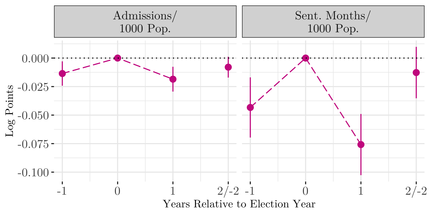
Figure C.1: Criminal Sentencing Outcomes,
Relative to District Attorney Election Year
– with Log Transformation (log(1+x))

Notes: Graph depicts dynamic difference-in-differences model estimates using Equation 2 (weighted to adjust for differences in sampling probabilities across districts and across time). Estimates are at the county level by year. The standard errors are corrected for correlation across district attorneys and over time in a given county by clustering at the district level. Estimates include state- and year- fixed effects. Vertical lines mark two standard errors. Estimates calculated relative to the election year value, which is normalized to 0. Log Transformation performed where each county’s outcome variable is incremented by 1 before taking the log.

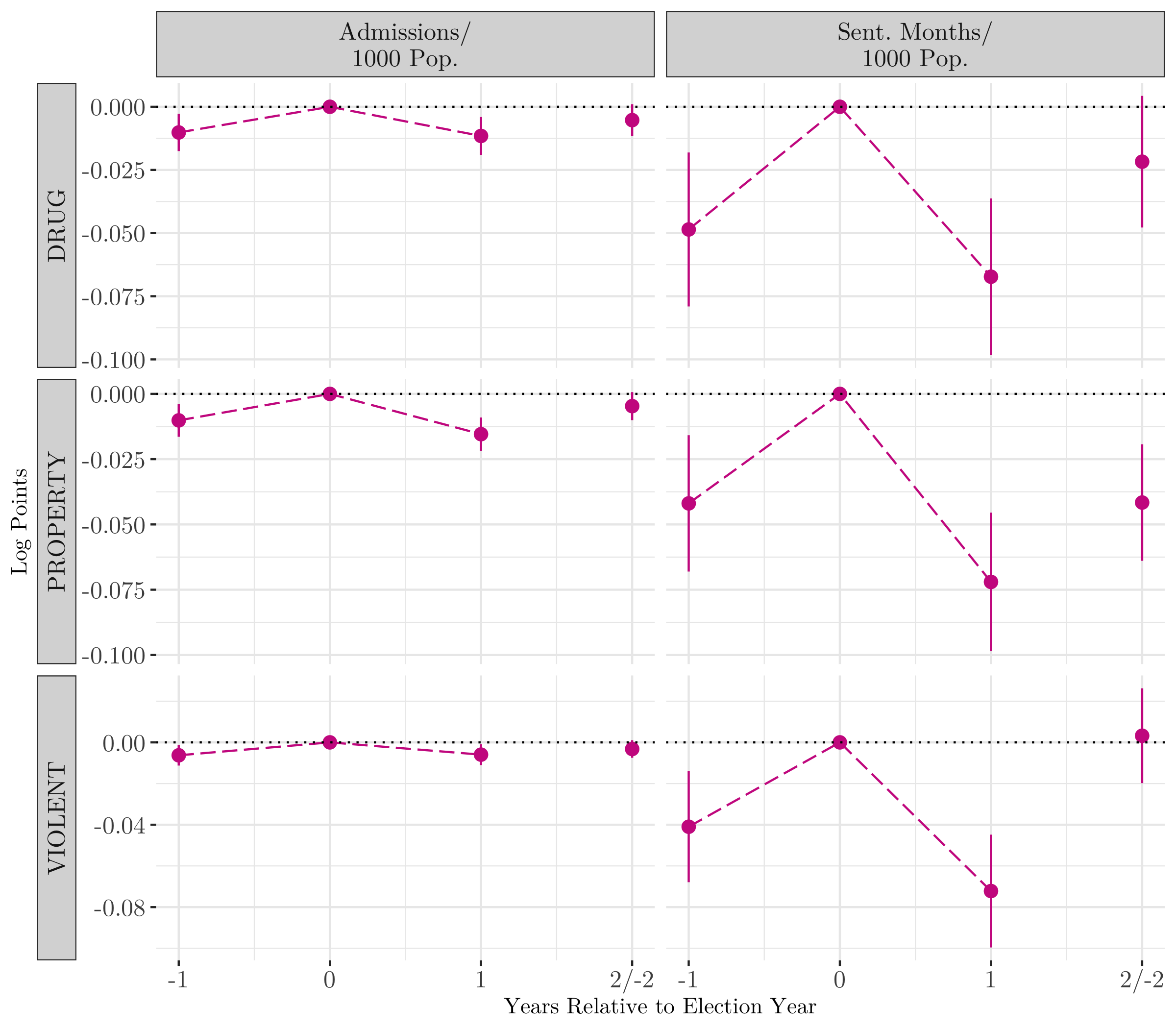
Figure C.2: Criminal Sentencing Outcomes,
Relative to District Attorney Election Year – Offense Subcategories
– with Log Transformation (log(1+x))

Notes: Graph depicts dynamic difference-in-differences model estimates using Equation 2 (population weighted to adjust for differences in sampling probabilities across districts and across time). Estimates are at the county level by year. The standard errors are corrected for correlation across district attorneys and over time in a given county by clustering at the district level. Estimates include state- and year- fixed effects. Vertical lines mark two standard errors. Estimates calculated relative to the election year value, which is normalized to 0. Log Transformation performed where each county’s outcome variable is incremented by 1 before taking the log.

Table C.5: Total Months Sentenced / 1000 Population, by Months from General Election (Property Offenses)

	Dependent variable (in Log Points)
	Months/1000 Pop.
-19	$-$0.009 (0.024)
-18	$-$0.011 (0.022)
-17	0.082∗∗∗ (0.022)
-16	$-$0.005 (0.026)
-15	$-$0.017 (0.021)
-14	$-$0.003 (0.021)
-13	0.005 (0.022)
-12	0.023 (0.021)
-11	0.027 (0.018)
-10	0.017 (0.019)
-9	0.026 (0.019)
-8	0.027 (0.019)
-7	0.076∗∗∗ (0.020)
-6	0.040∗ (0.021)
-5	0.055∗∗∗ (0.021)
-4	0.038∗ (0.021)
-3	0.061∗∗∗ (0.021)
-2	0.037∗∗ (0.018)
-1	0.045∗∗ (0.019)
0	0.014 (0.019)
1	0.011 (0.016)
2	$-$0.012 (0.018)
3	0.018 (0.018)
4	$-$0.022 (0.016)
5	$-$0.041∗ (0.024)
6	$-$0.031 (0.021)
7	0.026 (0.023)
8	0.011 (0.025)
9	$-$0.025 (0.021)
10	$-$0.010 (0.022)
11	0.008 (0.021)
12	0.001 (0.026)
Observations	256,764
	∗p$<$0.1; ∗∗p$<$0.05; ∗∗∗p$<$0.01

Notes: Table depicts dynamic difference-in-differences model estimates using Equation 2 (population weighted to adjust for differences in sampling probabilities across districts and across time). Estimates are at the county level by month. The standard errors are corrected for correlation across district attorneys and over time in a given county by clustering at the district level. Estimates include state- and year-month- fixed effects. Estimates calculated relative to omitted months in election cycle, which are normalized to 0.

Table C.6: Sentencing Outcomes, by Months from General Election (All Offenses)

	Dependent variable (in Log Points)
	Admissions/1000 Pop.	Months/1000 Pop.
	(1)	(2)
-19	0.003 (0.013)	$-$0.006 (0.017)
-18	$-$0.034∗∗ (0.014)	$-$0.018 (0.017)
-17	$-$0.001 (0.018)	0.013 (0.021)
-16	$-$0.034∗∗ (0.016)	$-$0.008 (0.018)
-15	$-$0.007 (0.015)	0.003 (0.018)
-14	0.018 (0.014)	0.009 (0.019)
-13	$-$0.001 (0.012)	$-$0.001 (0.017)
-12	0.003 (0.014)	0.001 (0.017)
-11	0.012 (0.015)	0.025 (0.018)
-10	0.024∗ (0.014)	0.010 (0.015)
-9	0.011 (0.011)	0.026∗ (0.014)
-8	0.029∗∗∗ (0.010)	0.031∗∗ (0.014)
-7	0.032∗∗ (0.013)	0.020 (0.015)
-6	0.018 (0.014)	0.017 (0.015)
-5	0.020 (0.015)	0.023 (0.018)
-4	0.010 (0.013)	0.020 (0.017)
-3	0.026∗∗ (0.013)	0.022 (0.015)
-2	0.020∗ (0.012)	0.014 (0.016)
-1	0.013 (0.013)	$-$0.001 (0.015)
0	0.003 (0.012)	0.001 (0.016)
1	0.021∗ (0.012)	0.008 (0.014)
2	$-$0.007 (0.015)	$-$0.025 (0.016)
3	$-$0.005 (0.013)	$-$0.014 (0.015)
4	$-$0.012 (0.013)	$-$0.014 (0.017)
5	0.005 (0.014)	$-$0.016 (0.017)
6	$-$0.047∗∗∗ (0.014)	$-$0.065∗∗∗ (0.016)
7	$-$0.009 (0.014)	$-$0.001 (0.017)
8	$-$0.041∗∗∗ (0.016)	$-$0.047∗∗ (0.019)
9	$-$0.015 (0.015)	$-$0.018 (0.018)
10	0.014 (0.016)	0.0001 (0.020)
11	0.005 (0.016)	0.004 (0.018)
12	0.007 (0.016)	$-$0.013 (0.019)
Observations	370,104	346,945
	∗p$<$0.1; ∗∗p$<$0.05; ∗∗∗p$<$0.01

Notes: Table depicts dynamic difference-in-differences model estimates using Equation 2 (population weighted to adjust for differences in sampling probabilities across districts and across time). Estimates are at the county level by month. The standard errors are corrected for correlation across district attorneys and over time in a given county by clustering at the district level. Estimates include state- and year-month- fixed effects. Estimates calculated relative to omitted months in election cycle, which are normalized to 0.

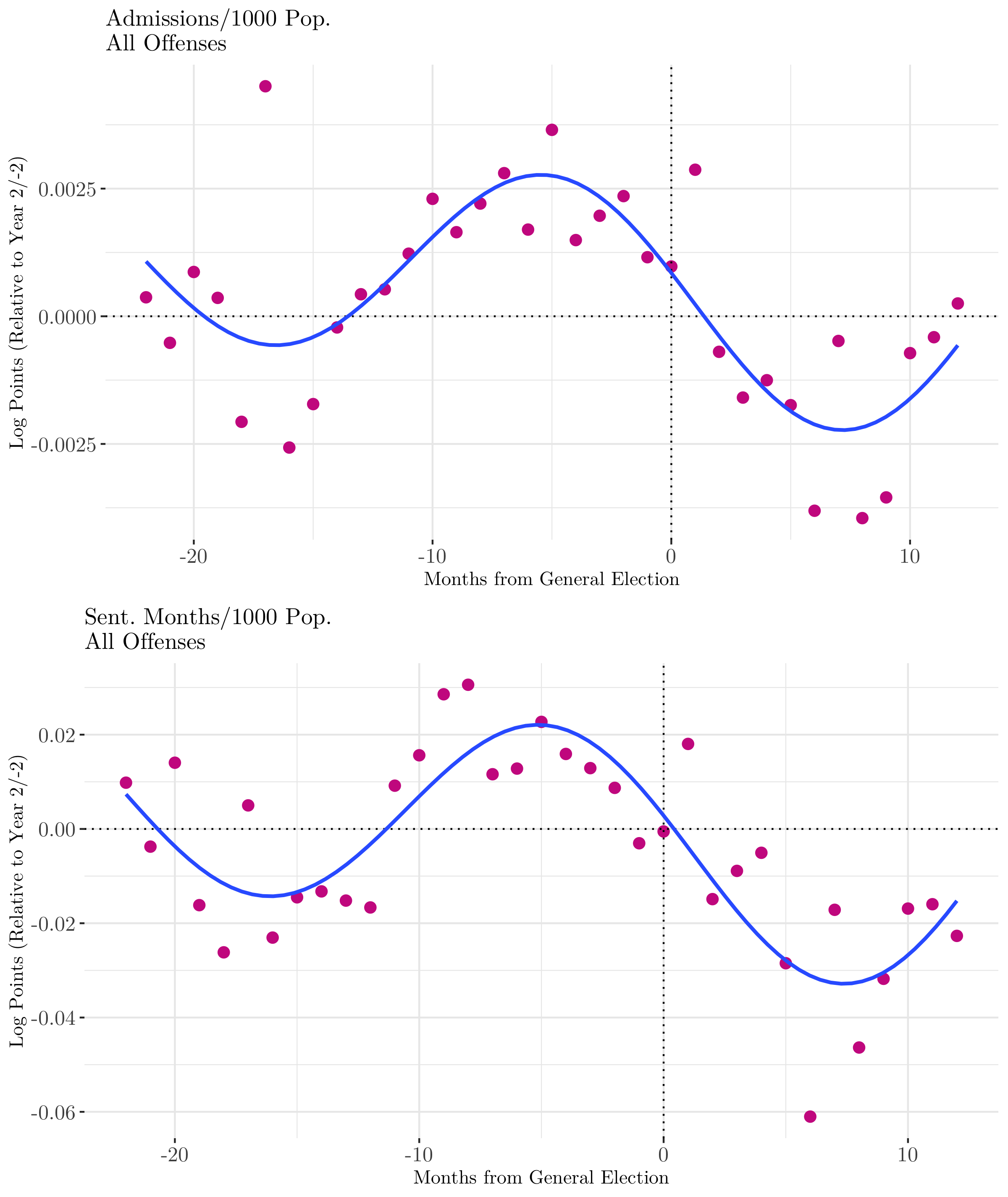
Figure C.3: Monthly Criminal Sentencing Outcomes in Election Cycle
– with Log Transformation (log(1+x))

Notes: Graph depicts dynamic difference-in-differences model estimates using Equation 2 (population weighted to adjust for differences in sampling probabilities across districts and across time). Estimates are at the county level by month. Estimates include state- and year-month- fixed effects. Vertical lines mark two standard errors. Estimates calculated relative to the months in year 2/-2 from an election year, which are normalized to 0. Best-fit line estimated via a sinusoidal model. Corresponding regression table is in Appendix. Log Transformation performed where each county’s outcome variable is incremented by 1 before taking the log.

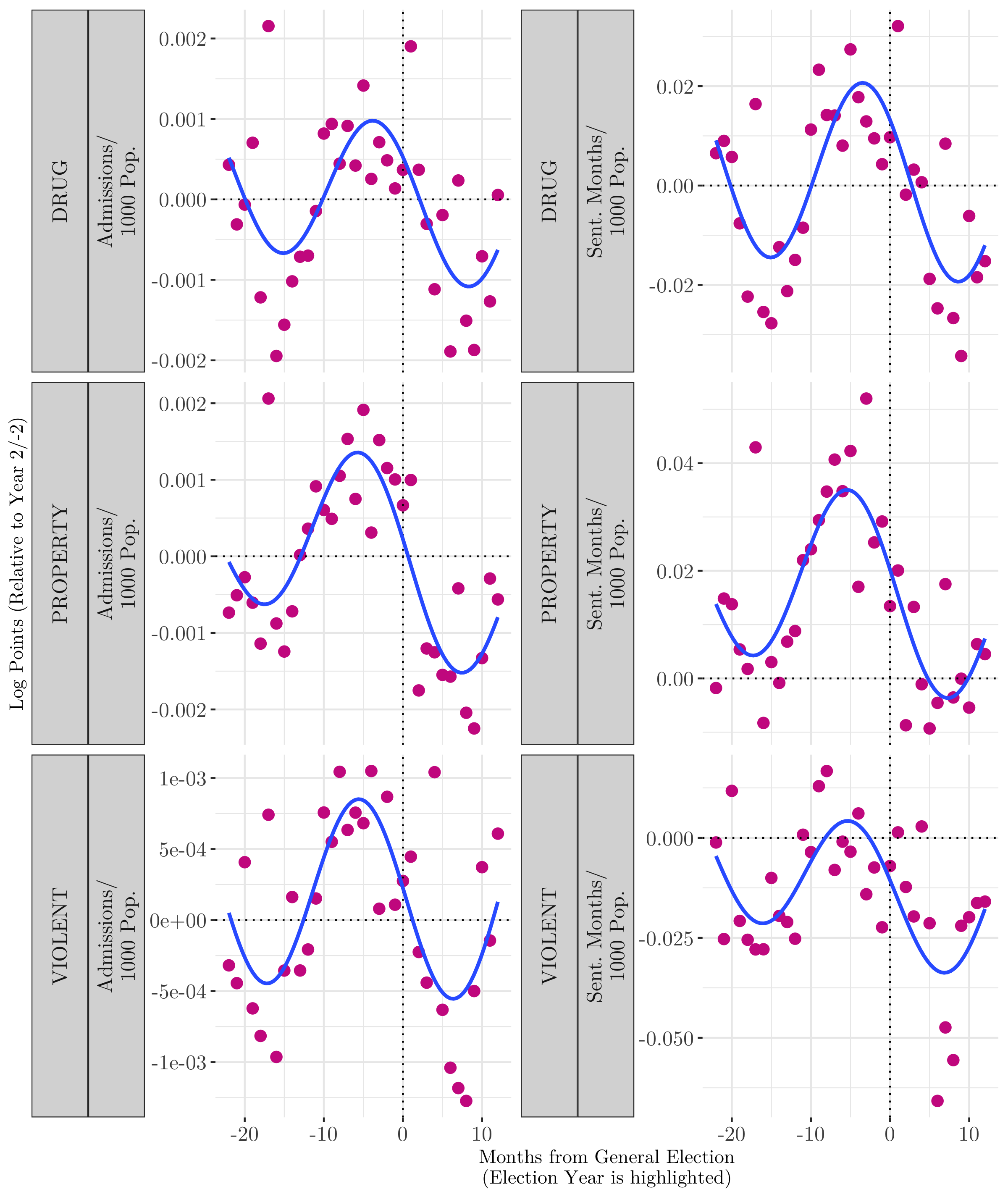
Figure C.4: Monthly Criminal Sentencing Outcomes in Election Cycle – Offense Subcategories
– with Log Transformation (log(1+x))

Notes: Graph depicts dynamic difference-in-differences model estimates using Equation 2 (population weighted to adjust for differences in sampling probabilities across districts and across time). Estimates are at the county level by month. Estimates include state- and year-month- fixed effects. Estimates calculated relative to the months in year 2/-2 from an election year, which are normalized to 0. Best-fit line estimated via a sinusoidal model. Corresponding regression tables are in Appendix. Log Transformation performed where each county’s outcome variable is incremented by 1 before taking the log.

Table C.7: Arrest and Crime Rates, by Years from Election Year

	Dependent variable (in Log Points)
	Crimes/1000 Pop.	Arrests/1000 Pop.
	(1)	(2)
-1	0.005 (0.011)	0.026 (0.030)
1	0.049∗∗ (0.019)	0.061 (0.047)
-2	0.026 (0.018)	0.076 (0.057)
Observations	37,451	36,189
	∗p$<$0.1; ∗∗p$<$0.05; ∗∗∗p$<$0.01

Notes: Table depicts dynamic difference-in-differences model estimates using Equation 2 (population weighted to adjust for differences in sampling probabilities across districts and across time). Estimates are at the county level by year. The standard errors are corrected for correlation across district attorneys and over time in a given county by clustering at the district level. Estimates include state- and year- fixed effects. Estimates calculated relative to the election year, which is normalized to 0.

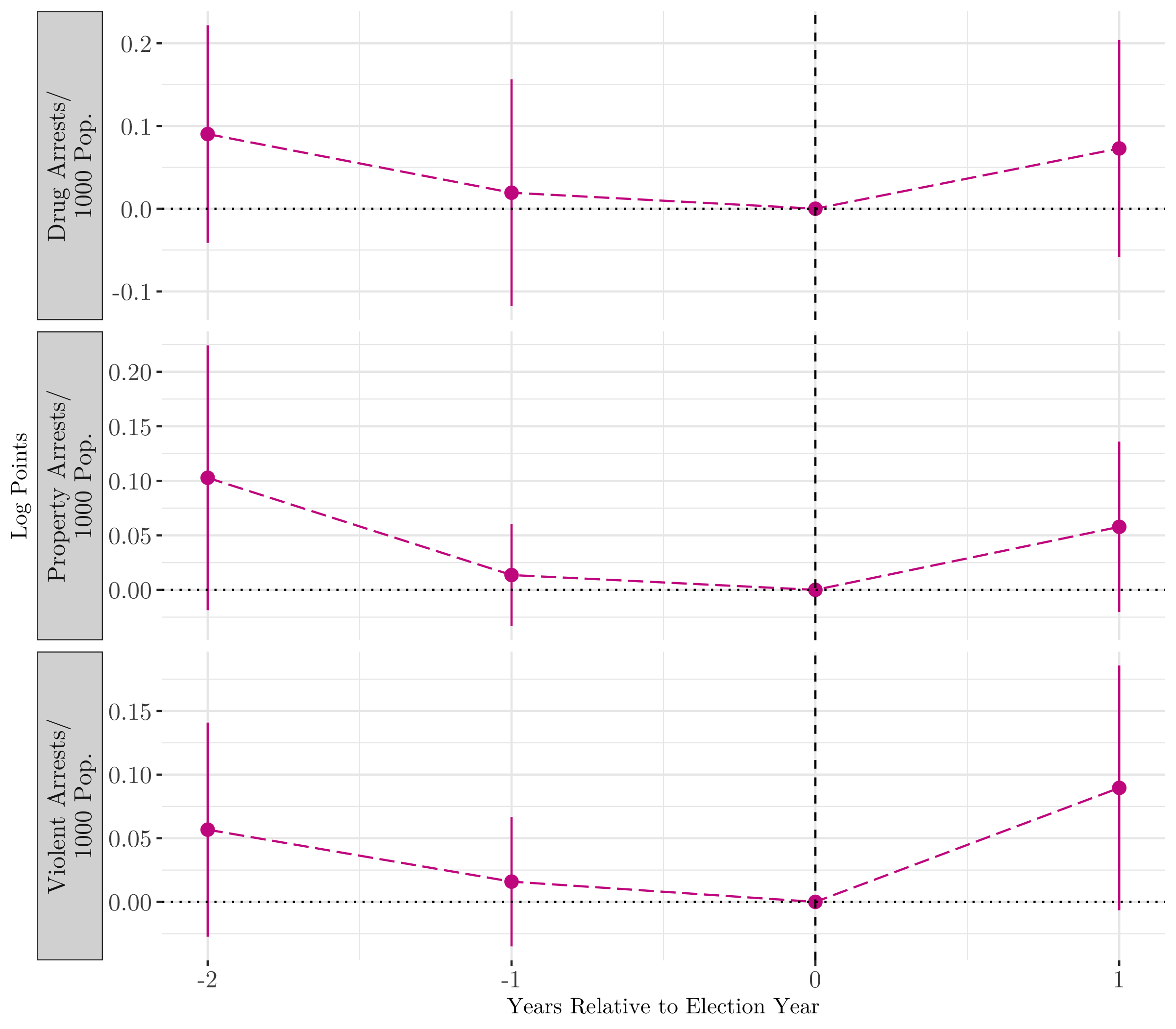
Figure C.5: Arrest Outcomes in Election Cycle – Offense Subcategories

Notes: Graph depicts dynamic difference-in-differences model estimates using Equation 2 (population weighted to adjust for differences in sampling probabilities across districts and across time). Estimates are at the county level by year. Estimates include state- and year fixed effects. Estimates calculated relative to the election year, which is normalized to 0.

References

- [1] Gregory A. and Sanford C Gordon “Accountability and Coercion: Is Justice Blind When it Runs for Office?” In American Journal of Political Science 48.2 Wiley Online Library, 2004, pp. 247–263
- [2] David Abrams, Roberto Galbiati, Emeric Henry and Arnaud Philippe “Electoral Sentencing Cycles” CEPR Discussion Paper No. DP14049, 2019
- [3] Scott Baker and Claudio Mezzetti “Prosecutorial Resources, Plea Bargaining, and the Decision to Go to Trial” In Journal of Law, Economics, and Organization 17.1 Oxford University Press, 2001, pp. 149–167
- [4] Siddhartha Bandyopadhyay and Bryan C McCannon “The Effect of the Election of Prosecutors on Criminal Trials” In Public Choice 161.1-2 Springer, 2014, pp. 141–156
- [5] Robert J Barro “The Control of Politicians: An Economic Model” In Public choice JSTOR, 1973, pp. 19–42
- [6] Justin Benedictis-Kessner “Off-Cycle and Out of Office: Election Timing and the Incumbency Advantage” In The Journal of Politics 80.1 University of Chicago Press Chicago, IL, 2018, pp. 119–132
- [7] Carlos Berdejó and Noam Yuchtman “Crime, Punishment, and Politics: An Analysis of Political Cycles in Criminal Sentencing” In Review of Economics and Statistics 95.3 MIT Press, 2013, pp. 741–756
- [8] David Bjerk “Making the Crime Fit the Penalty: The Role of Prosecutorial Discretion Under Mandatory Minimum Sentencing” In The Journal of Law and Economics 48.2 The University of Chicago Press, 2005, pp. 591–625
- [9] “Blakely v. Washington” 542 U.S. 296, 124 S. Ct. 2531, 159 L. Ed. 2d 403, 2004
- [10] Alfred Blumstein “Bringing Down the US Prison Population” In The Prison Journal 91.3_suppl SAGE Publications Sage CA: Los Angeles, CA, 2011, pp. 12S–26S
- [11] Adam Bonica “Database on Ideology, Money in Politics, and Elections (DIME)” Harvard Dataverse, 2015 DOI: 10.7910/DVN/O5PX0B
- [12] Raj Chetty et al. “The Opportunity Atlas: Mapping the Childhood Roots of Social Mobility”, 2018
- [13] Todd R Clear and James Austin “Reducing Mass Incarceration: Implications of the iron Law of Prison Populations” In Harv. L. & Pol’y Rev. 3 HeinOnline, 2009, pp. 307
- [14] Ernesto Dal Bó and Martín A Rossi “Term Length and the Effort of Politicians” In The Review of Economic Studies 78.4 Oxford University Press, 2011, pp. 1237–1263
- [15] Clement De Chaisemartin and Xavier d’Haultfoeuille “Two-way Fixed Effects Estimators with Heterogeneous Treatment Effects” In American Economic Review 110.9, 2020, pp. 2964–96
- [16] Christian Dippel and Michael Poyker “How Common are Electoral Cycles in Criminal Sentencing?” In National Bureau of Economic Research Working Paper, 2019
- [17] Andrew Dyke “Electoral Cycles in the Administration of Criminal Justice” In Public Choice 133.3-4 Springer, 2007, pp. 417–437
- [18] John Ferejohn “Incumbent Performance and Electoral Control” In Public choice 50.1 Springer, 1986, pp. 5–25
- [19] Joshua B Fischman and Max M Schanzenbach “Racial Disparities Under the Federal Sentencing Guidelines: The Role of Judicial Discretion and Mandatory Minimums” In Journal of Empirical Legal Studies 9.4 Wiley Online Library, 2012, pp. 729–764
- [20] Andrew Healy and Gabriel S Lenz “Substituting the End for the Whole: Why Voters Respond Primarily to the Election-Year Economy” In American Journal of Political Science 58.1 Wiley Online Library, 2014, pp. 31–47
- [21] Carissa Byrne Hessick and Michael Morse “Picking Prosecutors” In Iowa Law Review 105.4, 2020
- [22] Joshua Kleinfeld “Manifesto of Democratic Criminal Justice” In Nw. UL Rev. 111 HeinOnline, 2016, pp. 1367
- [23] Jack M Kress “Progress and prosecution” In The Annals of the American Academy of Political and Social Science 423.1 Sage Publications Sage CA: Thousand Oaks, CA, 1976, pp. 99–116
- [24] Sam Krumholz “The Effect of District Attorneys on Local Criminal Justice Outcomes” In Available at SSRN 3243162, 2019
- [25] William M Landes “An Economic Analysis of the Courts” In The Journal of Law and Economics 14.1 The University of Chicago Law School, 1971, pp. 61–107
- [26] Steven D Levitt “Why Do Increased Arrest Rates Appear to Reduce Crime: Deterrence, Incapacitation, or Measurement Error?” In Economic inquiry 36.3 Wiley Online Library, 1998, pp. 353–372
- [27] Steven D Levitt “Using Electoral Cycles in Police Hiring to Estimate the Effects of Police on Crime: Reply” In American Economic Review 92.4, 2002, pp. 1244–1250
- [28] Claire SH Lim, James M Snyder Jr and David Strömberg “The Judge, the Politician, and the Press: Newspaper Coverage and Criminal Sentencing Across Electoral Systems” In American Economic Journal: Applied Economics 7.4, 2015, pp. 103–35
- [29] Michael B MacKuen, Robert S Erikson and James A Stimson “Peasants or Bankers? The American Electorate and the US Economy” In The American Political Science Review JSTOR, 1992, pp. 597–611
- [30] Justin McCrary “Using Electoral Cycles in Police Hiring to Estimate the Effect of :olice on Crime: Comment” In American Economic Review 92.4, 2002, pp. 1236–1243
- [31] Terance D Miethe “Charging and Plea Bargaining Practices Under Determinate Sentencing: An Investigation of the Hydraulic Displacement of Discretion” In J. Crim. L. & Criminology 78 HeinOnline, 1987, pp. 155
- [32] David B Mustard “Racial, Ethnic, and Gender Disparities in Sentencing: Evidence from the US Federal Courts” In The Journal of Law and Economics 44.1 The University of Chicago Press, 2001, pp. 285–314
- [33] Melissa R Nadel, Samuel JA Scaggs and William D Bales “Politics in Punishment: The Effect of the State Attorney Election Cycle on Conviction and Sentencing Outcomes in Florida” In American journal of criminal justice 42.4 Springer, 2017, pp. 845–862
- [34] Derek Neal and Armin Rick “The Prison Boom and Sentencing Policy” In The Journal of Legal Studies 45.1 University of Chicago Press Chicago, IL, 2016, pp. 1–41
- [35] Jeffrey S Nowacki “Race, Ethnicity, and Judicial Discretion: The Influence of the United States v. Booker Decision” In Crime & Delinquency 61.10 SAGE Publications Sage CA: Los Angeles, CA, 2015, pp. 1360–1385
- [36] Emily Owens “The Economics of Policing” In Handbook of Labor, Human Resources and Population Economics Springer, 2020, pp. 1–30
- [37] John F Pfaff “The Micro and Macro Causes of Prison Growth” In Ga. St. UL Rev. 28 HeinOnline, 2011, pp. 1239
- [38] John Rappaport “Some Doubts About “Democratizing” Criminal Justice” In The University of Chicago Law Review 87.3 JSTOR, 2020, pp. 711–814
- [39] Eric Rasmusen, Manu Raghav and Mark Ramseyer “Convictions Versus Conviction Rates: the Prosecutor’s Choice” In American Law and Economics Review 11.1 Oxford University Press, 2009, pp. 47–78
- [40] M Marit Rehavi and Sonja B Starr “Racial Disparity in Federal Criminal Sentences” In Journal of Political Economy 122.6 University of Chicago Press Chicago, IL, 2014, pp. 1320–1354
- [41] Yianis Sarafidis “What Have You Done for Me Lately? Release of Information and Strategic Manipulation of Memories” In The Economic Journal 117.518 Oxford University Press Oxford, UK, 2007, pp. 307–326
- [42] Stephen J Schulhofer and Ilene H Nagel “Plea Negotiations Under the Federal Sentencing Guidelines: Guideline Circumvention and its Dynamics in the Post–Mistretta Period” In Nw. UL Rev. 91 HeinOnline, 1996, pp. 1284
- [43] Christian Schultz “Information, Polarization and Term Length in Democracy” In Journal of Public Economics 92.5-6 Elsevier, 2008, pp. 1078–1091
- [44] Ryan W Scott “Inter-Judge Sentencing Disparity After Booker: A First Look” In Stan. L. Rev. 63 HeinOnline, 2010, pp. 1
- [45] Lauren O’Neill Shermer and Brian D Johnson “Criminal Prosecutions: Examining Prosecutorial Discretion and Charge Reductions in US Federal District Courts” In Justice Quarterly 27.3 Taylor & Francis, 2010, pp. 394–430
- [46] Tom W Smith, Michael Davern and Jeremy Freese “General Social Surveys, 1972-2016 [machine-readable data file]/Principal Investigator, Smith, Tom W.; Co-Principal Investigators, Peter V. Marsden and Michael Hout; Sponsored by National Science Foundation” In Chicago: NORC, 2018
- [47] Don Stemen, Andres Rengifo and James Wilson “Of Fragmentation and Ferment: The Impact of State Sentencing Policies on Incarceration Rates, 1975-2002” Vera Institute of Justice New York, 2005
- [48] Kate Stith “The Arc of the Pendulum: Judges, Prosecutors, and the Exercise of Discretion” In Yale LJ 117 HeinOnline, 2007, pp. 1420
- [49] Liyang Sun and Sarah Abraham “Estimating dynamic treatment effects in event studies with heterogeneous treatment effects” In Journal of Econometrics Elsevier, 2020
- [50] Daniel M Thompson “Replication Data for: How Partisan Is Local Law Enforcement? Evidence from Sheriff Cooperation with Immigration Authorities” Harvard Dataverse, 2020 DOI: 10.7910/DVN/CFASH6
- [51] Ronald Wright and Marc Miller “The Screening/Bargaining Tradeoff” In Stanford Law Review JSTOR, 2002, pp. 29–118
- [52] Ronald F Wright “Beyond Prosecutor Elections” In SMUL Rev. 67 HeinOnline, 2014, pp. 593