The Open University of Israelnutov@openu.ac.il https://orcid.org/0000-0002-6629-3243 \CopyrightZeev Nutov \ccsdesc[100]Theory of computation Design and analysis of algorithms
Acknowledgements.
Data structures for connectivity and cut queries
Abstract
Let denote the maximum number of internally disjoint -paths in an undirected graph . We consider designing a compact data structure that answers -bounded node connectivity queries: given return . A trivial data structure has space and query time . A data structure of Hsu & Lu [8] has space and query time , and a randomized data structure of Iszak & Nutov [9] has space and query time . We extend the Hsu-Lu data structure to answer queries in time . In parallel to our work, Pettie, Saranurak & Yin [19] extended the Iszak-Nutov [9] data structure to answer queries in time . Our data structure is more compact than that of [19] for , and our query time is always better.
We then augment our data structure by a list of cuts that enables to return a pointer to a minimum -cut in the list (or to a cut of size ) whenever . A trivial data structure has cut list size , and cut query time , while the Pettie, Saranurak & Yin [19] data structure has list size and cut query time . We show that cuts suffice to return an -cut of size , and a list of cuts contains a minimum -cut for every .
In the case when is a node subset with for all , we show that cuts suffice, and that these cuts can be partitioned into laminar families. Thus using space we can answers each connectivity and cut queries for in time, generalizing and substantially simplifying the proof of a result of Pettie and Yin [20] for the case .
keywords:
node connectivity, minimum cuts, data structure, connectivity queries1 Introduction
Let denote the maximum number of internally disjoint -paths in a graph . An -cut is a subset such that has no -path. By Menger’s Theorem, equals to the minimum size of an -cut, and there always exists a minimum -cut that contains no edge except of . We consider designing a compact data structure that given and answers the following -bounded connectivity/cut queries.
| pcon | (partial connectivity query): | Determine whether . |
| pcut | (partial cut query): | If then return an -cut of size . |
| con | (connectivity query): | Return . |
| cut | (min-cut query): | If then return a minimum -cut. |
The cut queries pcut and cut require time just to write an -cut. It is therefore makes sense to allow the data structure to include a list of cuts, and to return just a pointer to an -cut in the list. How short can this list be? By choosing a minimum -cut for each pair , one gets a list of cuts. This gives a trivial data structure, that answers queries in time, but has cuts – just store the pairwise connectivities in an matrix, with relevan pointers to cuts. For edge connectivity, the Gomory-Hu Cut-Tree [6] shows that there exists such a list of cuts that form a laminar family. However, no similar result is known for the node connectivity case considered here.
Hsu and Lu [8] showed that for any graph there exists an auxiliary graph and an ordered partition of , such that the following holds:
-
•
In , every part has at most neighbors in ; hence .
-
•
iff belong to the same part of or .
They also gave a polynomial time algorithm for constructing such and . Augmenting by a perfect hashing data structure enables to answer ”?” queries in time. Since , this gives an space111As in previous works, we ignore the unavoidable factor invoked by storing the indexes of nodes, and assume that any basic arithmetic or comparison operation with indexes can be done in time. data structure that determines whether in time. Furthermore, a collection of such data structures for each has space and enables to find in time, using binary search. We improve the query time to .
Theorem 1.1.
There exists an space data structure that answers con queries in time.
Our data structure is easy to describe. Let be a tree rooted at with leaf set and integer levels such that and if is a child of ; we will call such a pair a leveled tree. Let denote the lowest common ancestor of in . Our data structure for answering con queries is described in the following theorem.
Theorem 1.2.
For any graph and a positive integer there exist a leveled tree with leaf set and edges, and an edge weighted graph with edges, such that the following holds:
Augmenting by Gabow & Tarjan [5] lowest common ancestor data structure enables to find in time. Augmenting by a perfect hashing data structure enables in time to return or to determine that . Since , this gives an space data structure that answers con queries in time, as required in Theorem 1.1.
In parallel to our work, Pettie, Saranurak, & Yin [19] extended the randomized space data structure of Izsak & Nutov [9], that in turn is based on an idea of Chuzhoy and Khanna [2]. The Izsak & Nutov data structure answer con queries in time, and Pettie, Saranurak, & Yin extended it to answer con queries in time. We briefly describe these results. Given a set of terminals, the edges and the nodes in are called elements. The element connectivity between is the maximum number of pairwise element disjoint -paths. The Gomory-Hu tree extends to element connectivity (c.f. [21, 1]), and implies an space data structure that answers element connectivity queries between terminals in time. The data structure of [9] decomposes a node connectivity instance into element connectivity instances with terminals each; we will give a generalization of this decomposition in Section 5. For any element connectivity instance with terminal set and , is at most the element -connectivity in , and for at least one instance an equality holds (an instance with and for some minimum -cut ). So, to find , one has to find the minimum element -connectivity, among all instances in which are terminals. There are element connectivity instances, with terminals each, hence the overall number of terminals is . Iszak and Nutov [9] considered designing a labeling scheme222For additional work on labeling schemes for node connectivity, see for example, [11, 12, 8]., where efficient query time is not required, and used the connectivity classes data structure in each element connectivity instance; this enables to answer con queries in time. Pettie, Saranurak, and Yin [19] used element connectivity Gomory-Hu trees instead, and also designed a novel data structure that given finds an instance with the minimum element -connectivity in time. They also showed that for large values of , any data structure for answering node connectivity queries needs at least space, matching up to an factor the space of a sparse certificate graph [15].
Let us compare between the [19] space data structure to our results. Our query time is always better than that of [19] – vs. , and we use less space for . Note that for are known linear space data structures that can answer cut queries in time; see [7] and [10] for the cases and , respectively. Our work, that was done independently from [19] and uses totally different techniques, extend this to any constant , bridging the gap between the result of [19] and the results known for . See Table 1 for comparison between some data structures.
| space | con | list size | cut | reference |
|---|---|---|---|---|
| folklore | ||||
| - | [15] | |||
| - | - | [8] | ||
| [19] | ||||
| this paper |
A graph is -connected if for all . Recently, Pettie and Yin [20], and earlier in the 90’s Cohen, Di Battista, Kanevsky, and Tamassia [3], considered the above problem in -connected graphs. Pettie and Yin [20] suggested for an space data structure, that answers con in time and cut in time; they showed that it can be constructed in time. The arguments in [20] are complex, and here by a simpler proof we obtain the following generalization as well as an improvement on the cut query. For a set of terminals we say that a graph is --connected if for all . We will improve over Theorem 1.1 for --connected graphs as follows.
Theorem 1.3.
For any --connected graph with , there exists an space data structure, that includes a list of cuts, and answers con and cut queries for node pairs in in time.
Theorem 1.4.
There exists an space data structure that includes a list of cuts, that answers con and pcut queries in time; a list of cuts and space enables to answer also cut queries in time.
We note that the [19] data structure can be augmented by a list of cuts to support cut queries in time . Our query time is always better, and our cut list size is better when . Furthermore, if we want to answer only pcut queries, then our list size is , which is smaller than the cut list size of [19].
All our data structures can be constructed in polynomial time; we will not discuss designing efficient construction algorithms here and leave this for future work.
2 Connectivity queries in general graphs (Theorem 1.2)
We start by describing a simple data structure for answering edge connectivity queries. Let denote the maximum number of edge disjoint -paths in . For let us define the relation . It is known that is an equivalence relation and its equivalence classes are called classes of -edge-connectivity, or just -classes for short. Let denote the partition of into -classes. One can see that if then , and this implies that is a refinement of . Consequently, the partitions form a laminar (multi-)family and can be represented by by a leveled rooted tree as follows:
-
•
The nodes of each level are the parts of .
-
•
The parent of a part is the part that contains .
We may add the partition into singletons as level , and assume that the leaf set of is . Note that then , where is the the distance of a node of to the root. Thus augmenting by Gabow & Tarjan [5] lowest common ancestor data structure enables to find in time. Note that has edges. The size of can be reduced to by shortcutting nodes that have a unique child, so we will get a leveled tree of size . And since the parameter has no role in the size of , we may set and obtain .
The reader may observe that this data structure is not really related to connectivity, as it does not use any special property (e.g., submodularity) of the cut function. Let us illustrate this on a more general setting. We say that is an -set if and . Let be an arbitrary non-negative integer valued set function on subsets of . Let us define the -connectivity between by . W.l.o.g. we may assume that is symmetric, namely, that for all , as otherwise we may consider the function . Note that then . By the same method we just described, one can deduce the following.
Corollary 2.1.
For any set function on there exist a leveled tree with leaf set and edges such that for any .
We emphasize again that the above corollary is valid for any set function. For edge connectivity, the appropriate set function is given by , where is the set of edges in with exactly one end in .
While a natural way to represent an edge cut of a graph is by a node subset, for node cuts we need a more general object given in the following definition.
Definition 2.2.
A biset on a groundset is an ordered pair such that ; is the inner part and is the outer part of , is the cut of , is the co-set of , and is the co-biset of . We say that is an -biset if and .
Let be an arbitrary biset function on a groundset . W.l.o.g. we will assume that is symmetric, namely, that for all . Given (a value oracle for) such we define the -connectivity between by
For node connectivity of a given graph , an appropriate biset function is given by , where here is the set of edges in with one end in and the other in . We will prove the following generalization of Theorem 1.2.
Theorem 2.3.
For any biset function on and a positive integer there exist exists a leveled tree with edges and an edge weighted graph with edges, where , such that for any the following holds:
| (1) |
To see that Theorem 2.3 implies Theorem 1.2, note that if then , and thus for this case both theorems coincide.
In the rest of this section we prove Theorem 2.3. We may assume that is symmetric, namely, that for every biset ; otherwise, we may consider the function . We will start with a simpler task – given a set family and , design a data structure that determines for whether there exists and -biset .
Definition 2.4.
Let be a symmetric biset family on . We say that are -inseparable if has no -biset. The -inseparability graph of has node set and edge set .
One can observe that for any , if is the -separability graph of then is the -separability graph of . The following lemma was proved by Hsu & Lu in [8] for the particular case when for a given a graph ; the proof for an arbitrary (symmetric) biset family is similar.
Lemma 2.5.
Let be a symmetric biset family on and let be the -inseparability graph of . There exists an ordered partition of such that in each is a clique with at most neighbors in , where . Consequently, if is the set of edges in that do not belong to any clique then .
Proof 2.6.
We first show that has a clique with at most neighbors. The algorithm for finding such a clique is as follows.
We show that the algorithm is well defined.
-
•
The condition of the while-loop implies the existence of and in step 3 and also of in step 4 (since is symmetric).
-
•
Step 5 removes some node from but also keeps some node in . Hence the while-loop terminates in at most iterations and at the end of the algorithm.
It remains to show that has at most neighbors. Let and at the end of iteration . By steps 4,5,6 in the algorithm, , where is the biset chosen at iteration . Now we continue by induction. Clearly, . For the induction step assume that . Then
Since are integers we get , as claimed.
Now we show that has an ordered partition as in the lemma. The algorithm for obtaining such is as follows.
Since at any step of Algorithm 2, has at most neighbors in , the lemma follows.
We now finish the proof of Theorem 2.3. Let and let be the -inseparability graph of , . Note that and thus . The algorithm starts with the -level ordered partition and continues with iterations. At the beginning of iteration we already have an -level ordered partition of . For each part of we compute an ordered partition of and an edge subset of as in Lemma 2.5 with and . We then concatenate the computed partitions into one ordered partition and let . Note that , hence . For each we let ; note that and that an inequality may hold.
Note that is a refinement of . We augment the partitions by the partition into singletons, and represent the obtained sequence of partitions by a leveled tree of size , as was described at the beginning of this section for the edge connectivity case. In addition, we let , so .
3 Connectivity and cut queries in k-S-connected graphs (Theorem 1.3)
We start by giving a simple proof for a slight improvement of Theorem 1.3 for the case . This case was considered by Pettie-Yin in [20], but our data structure and arguments are substantially simpler than those in [20]. Here, and in other parts of the paper we will need the following known lemma, for which we provide a proof for completeness of exposition.
Lemma 3.1.
Let be a directed graph of maximum indegree . Then the underlying graph of is -colorable, and such a coloring can be computed in linear time.
Proof 3.2.
Since the indegree of every node in is at most , every subgraph of the underlying graph of has a node of degree . A graph is -degenerate if every subgraph of it has a node of degree . It is known that any -degenerate graph can be colored with colors, in linear time, see [4, 14]. This implies that the underlying graph of can be colored with colors in linear time.
Lemma 3.3.
For any -connected graph there exists an space data structure with a list of cuts that answers con and cut queries in time.
Proof 3.4.
Let be the set of nodes of degree in . If then is a minimum -cut for all . There are such minimum cuts. This situation can be recognized in time, hence assume that . Let be the set of edges such that and . By Mader’s Critical Cycle Theorem [13], is a forest, so . Thus just specifying the nodes in and edges in and a list of minimum -cuts gives an space data structure that answers the relevant queries in time.
Henceforth assume that and . We will show that then there exists a list of cuts, such that whenever there exists a minimum -cut in the list. We will also show how to choose the right minimum cut from the list in time.
Let denote the “node complement” of . We say that is: a tight set if and , an -set if and , and a small set if . Note that is tight if and only if is a minimum cut of , and is a union of some, but not all, connected components of . The following statement is a folklore, c.f. [16, 17].
Claim 1.
Let be tight sets. If the sets are both nonempty then are both tight. If are small sets and then is tight.
Let . For let be the (unique, by Claim 1) inclusion minimal small tight set that contains . Let . We claim that the family is a ”short” list of minimum cuts, that for every with includes a minimum -cut. Specifically, we claim that if an only if at least one of the following holds:
-
(i)
and is an -set, or
-
(ii)
and is a -set.
Indeed, if (i) holds then is a minimum -cut, while if (ii) holds then is a minimum -cut. Thus if (i) or (ii) holds. Assume now that and we will show that (i) or (ii) holds. Let be a minimum -cut. Then one component of contains and the other contains . Since , one of , say is small. Thus . Since and since , we have . Consequently, is a minimum -cut, as required.
Finally, we will show that can be partitioned into at most laminar families. Consider two sets and that are not laminar. Then since otherwise by Claim 1 is a (small) tight set that contains , contradicting the minimality of . By a similar argument, . We also cannot have both and , as then by Claim 1 is a tight set that contains , contradicting the minimality of . Consequently, or . Construct an auxiliary directed graph on node set and edges set . The indegree of every node in is at most . By Lemma 3.1, we can compute in polynomial time a partition of into at most independent sets. For each independent set , the family is laminar.
Our data structure for pairs with consists of:
-
•
A family of at most trees, where each tree with a mapping represents one of the at most laminar families of tight sets as; the total number of edges in all trees in is at most .
-
•
For each tree , a linear space data structure that answers ancestor/descendant queries in time. This can be done by assigning to each node of the in-time and the out-time in a DFS search on .
-
•
A list of minimum cuts; this can be also encoded by an auxiliary directed graph with edge set . Using perfect hashing data structure we can check whether in time.
For every let be the (unique) tree in where is represented. A direct consequence of (i) and (ii) above specifies how we answer the queries.
-
(i)
If in , is not a descendant of and , then is a minimum -cut.
-
(ii)
If in , is not a descendant of and , then is a minimum -cut.
If none of (i),(ii) holds then .
It is easy to see that with appropriate pointers, and using perfect hashing data structure to check adjacency in the auxiliary directed graph , we get an space data structure that checks the conditions above in time. If one of the conditions holds, the data structure return a pointer to one of or . Else, it reports that .
This concludes the proof of the lemma.
In the rest of this section let be a --connected graph with . Our proof of Theorem 1.3 uses ideas similar to those in the proof of Lemma 3.3, but it is substantially more involved. One reason is that we cannot use Mader’s Critical Cycle Theorem [13]. Another reason is that for the simpler case we could relate cuts to node subsets, but for the more general subset -connectivity case, we again need to consider bisets. Here we will say that is a tight biset if , , and , where is the set of edges in that go from to . Note that is tight if and only if is a minimum -cut for some and . We will consider the family obtained by projecting the tight bisets on . Note that for there might be many tight bisets in whose projection on is , and that there always exists at least one such biset.
Definition 3.5.
The intersection and the union of two bisets are the bisets defined by and . The biset is defined by . We say that : intersect if , cross if and , and co-cross if and .
We say that is a small biset if , and is a large biset otherwise. Clearly, for all . The family has the following properties, c.f. [16, 17].
Lemma 3.6.
The family has the following properties:
-
1.
is symmetric: whenever .
-
2.
is crossing: whenever cross.
-
3.
is co-crossing: whenever co-cross.
-
4.
If are small intersecting bisets then .
Definition 3.7.
We say that a biset contains a biset and write if and . are laminar if one of them contains the other or if . A biset family is laminar if its members are pairwise laminar.
For every let be the family of all inclusion minimal bisets with and . Let . Note that and that can be computed using min-cut computations. The following observation follows from the symmetry of .
Lemma 3.8.
Let be an -biset. If then there is an -biset in , and if then there is a -biset in . Consequently, for any , the family contains an -biset or a -biset.
The next lemma shows that if .
Lemma 3.9.
For any , contains at most one small biset and at most large bisets. In particular, if then in there are at most two large bisets and .
Proof 3.10.
In there is at most one small biset, by property 4 in Lemma 3.6. No two large bisets cross, as otherwise and (by property 2 in Lemma 3.6) , contradicting the minimality of . Thus the sets in are pairwise disjoint. Furthermore, for every large biset . This implies that the number of large bisets in is at most if .
By a proof similar to the one of Lemma 3.3 we have the following.
Lemma 3.11.
The family of small bisets in can be partitioned in polynomial time into at most laminar families.
Proof 3.12.
Consider two small bisets and that are not laminar. Then since otherwise , contradicting the minimality of . Similarly, . We also cannot have both and , as then co-cross and thus , contradicting the minimality of . Consequently, or . Construct an auxiliary directed graph on node set and edges set . The indegree of every node in is at most . By Lemma 3.1, we can compute in polynomial time a partition of into at most independent sets. For each independent set , the family is laminar.
Later, we will prove the following.
Lemma 3.13.
If then the family of large bisets in can be partitioned in polynomial time into at most laminar families.
Lemmas 3.11 and 3.13 imply that can be partitioned into at most laminar families. For our purposes, we just need the family of the inner sets of each family to be laminar. Together with Lemma 3.9 this implies Theorem 1.2 by the same way as in the proof of Lemma 3.3, except the following minor differences.
-
•
Here we have laminar families instead of laminar families, and for each we have by Lemma 3.9 instead of .
-
•
For each biset , our list of cuts will include a mixed cut of some tight biset of whose projection on is .
These differences affect space and query time only by a small constant factor. Thus all we need is to prove Lemma 3.13, which we will do in the rest of this section.
Lemma 3.14.
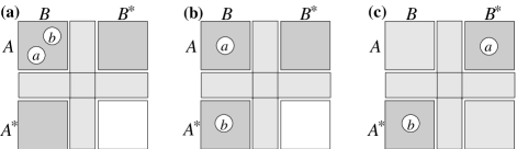
Let and be two non-laminar large bisets in . If then or , or (see Fig. 1(a)): , , and both are non-empty.
Proof 3.15.
Assume that and . We will show that then the case in Fig. 1(a) holds.
Suppose that ; the analysis of the case is similar. Then ; otherwise, cross and (by property 2 in Lemma 3.6) we get , contradicting the minimality of . Furthermore, if we get , contradicting that . By a similar argument, . If and (Fig. 1(b)), then co-cross (by property 3 in Lemma 3.6) and thus ; this contradicts the minimality of .
If none of is in , then (see Fig. 1(c)) and . Consequently, -co-cross, and thus (by property 3 in Lemma 3.6) , contradicting the minimality of .
Thus the only possible case is the one in Fig. 1(a), completing the proof of the lemma.
Corollary 3.16.
The family of large bisets in can be partitioned in polynomial time into at most parts such that any two bisets and that belong to the same part are either laminar, or have the following property: and .
Lemma 3.17.
Let be one of the parts as in Corollary 3.16; in particular, if are not laminar then and . Then can be partitioned in polynomial time into at most laminar families.
Proof 3.18.
Let be the family of maximal members in . We will show later that the set family has a hitting set of size . Now note that:
-
•
For every the family is laminar, since for any , while for any non-laminar .
-
•
Since is a hitting set of , for any there is , and then .
Summarizing, each one of the families is laminar and . By removing bisets that appear more than once, we get a partition of into laminar families.
It remains to show that has a hitting set of size . A fractional hitting set of is a function such that for all . For let be the family of sets in that contain , and let . Note that:
-
•
for all is a fractional hitting set of and .
-
•
No two bisets in intersect and . This implies , so for all .
Since for all , computing a minimum hitting set of reduces to the minimum Edge-Cover problem, and has a hitting set of size ( is the integrality gap of the Edge-Cover problem). Since , has a hitting set of size .
4 Cut queries in general graphs (Theorem 1.4)
In the first part of Theorem 1.4 we need to design an space data structure with a list of cuts, that answers con and pcut queries in time. We can use our -space data structure from Theorem 1.1 to answer con queries. To answer pcut queries, we combine our data structure for --connectivity in Theorem 1.3 with the Hsu-Lu [8] data structure. Recall that the [8] data structure consists of an auxiliary graph with edges and an ordered partition of , such that iff belong to the same part of or . Overall, the [8] data structure can be implemented using space and answers pcon queries in time.
We augment the Hsu & Lu [8] data structure by adding to each part a data structure for subset --connectivity; we add Theorem 1.3 data structure if , and the trivial data structure (an matrix) if . Then, by Theorem 1.3 for each part we have the following:
-
•
If then the cut list size is and the other parts use space .
-
•
If then the cut list size is and the other parts use space .
The total size of the cut list is bounded by , and thus uses space. The size of the other parts is . Thus the total size is due to the space required to store the cut list. Overall, we use space and cut list size, as required.
In the second part of Theorem 1.4 we need to show that increasing the cut list size to ans space to enables also to answer cut queries in time. For that, we can combine our data structures in Theorems 1.1 and 1.3. Instead of one clique partition, the Theorem 1.1 data structure has clique partitions, and in addition, . Thus compared to the first part, the cut list size increases by a factor of and so is the total space. This gives the second part of Theorem 1.4, and thus the proof of Theorem 1.4 is complete.
We can slightly improve the bound on the cut list sizes by a direct short proof, as follows.
Lemma 4.1.
There exists a list of at most cuts that contains an -cut of size for any with . Consequently, there exists a list of at most cuts that contains a minimum -cut for any with .
Proof 4.2.
The second part of the lemma easily follows from the first part. Note that the union of list as in the first part for every is a list that includes a minimum -cut for any with . The size of this list is .
We now prove the first part of the lemma. For a biset let . Here we will say that is an -tight biset if is an -biset and . Note that then is a minimum -cut, and that for any minimum -cut there exists an -tight biset with . It is known that the function satisfies the submodular inequality , and (by symmetry) also the co-submodular inequality .
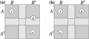
It is known that if are both -tight then so are . Let denote the (unique) inclusion minimal -tight biset. For let . Let be the family of all inclusion minimal bisets in the family . Let . One can verify that for any with , contains and -biset or a -biset with . We will show that for all .
Consider distinct bisets and in We claim that then or . Suppose to the contrary that and . If one of is in , say (see Fig. 2(a)), then is an -biset and is an -biset.Thus
Hence equality holds everywhere, so is -tight. This contradicts the minimality of .
Else, and (see Fig. 2(b)). Then is a -biset and is an -biset.Thus
Hence equality holds everywhere, so is -tight and is -tight. This implies and , and we get the contradiction .
From this we get that for all . To see this, construct an auxiliary directed graph on node set and edge set . Note that if has no edge between and then . The indegree of every node in is at most . Thus by Lemma 3.1 we get that the underlying graph of is -colorable, and thus can be partitioned into at most independent sets. For each independent set , the family consists of a single biset.
This concludes the proof of the lemma.
5 Decomposition of node connectivity into element connectivity
Recall that given a set of terminals, the element connectivity between is the maximum number of pairwise element disjoint -paths, where elements are the edges and the nodes in . Let denote the -element connectivity in . By Menger’s Theorem, equals the minimum size of a set of elements with such has not -path. It is easy to see that , and that an equality holds iff there exists a minimum -cut with . We thus will consider the following problem: given a family of subsets of , find a “small” family of subsets of such that for every and with , there is with and ; following [2], we will call such a family -resilient. The objective can be also to minimize . Chuzhoy and Khanna [2] showed that if is the family of all subsets of size , then there exists a -resilient family of size . They also gave a randomized polynomial time algorithm for finding such . The number of subsets of size is , while the relevant family in our case – as in Lemma 4.1, has a much smaller size . We will consider the case of an arbitrary family , and prove the following.
Lemma 5.1.
Let be a family of sets of size at most each on a groundset of size . Then there exists a -resilient family of subsets of of size each. Furthermore, assigning to each set in probability and applying randomized rounding times gives such w.h.p.
Proof 5.2.
If , then the subsets of of size is a family as required of size , so assume that .
Let and . Define a bipartite graph with sides by connecting to if and ; in this case we will say that covers . This defines an instance of the Set Cover problem, where are the sets and are the elements. The lemma says that there exists a cover of that has size .
A fractional cover of is a function such that
The value of a fractional cover is . It is known that if there is a fractional cover of value , then there is a cover of size . We have , hence and .
Our next goal is to show that there is a fractional cover of value . We have . The number of sets in that cover a given member is , which is the number of choices of a set of size from the set of size . Defining for all gives a fractional cover of value . Denote . Then:
Note that for we have . Let us choose such that , so ; assume that is an integer, as adjustment to floors and ceilings only affects by a small amount the constant hidden in the term. Since we obtain
Since we assume that , we have and thus . Consequently, we get that . This implies that a standard greedy algorithm for Set Cover, produces the required family of size . There is a difficulty to implement this algorithm in time polynomial in (unless is a constant), since may not be polynomial in . Thus we use a randomized algorithm for Set Cover, by rounding each entry to with probability determined by our fractional cover. It is known that repeating this rounding times gives a cover w.h.p., and clearly its expected size is times the value of the fractional hitting set. In our case, for all . Thus we just need to assign to each set in probability , and apply randomized rounding times.
References
- [1] C. Chekuri, T. Rukkanchanunt, and C. Xu. On element-connectivity preserving graph simplification. In 23rd European Symposium on Algorithms (ESA), pages 313–324, 2015.
- [2] J. Chuzhoy and S. Khanna. An -approximation algorithm for vertex-connectivity survivable network design. Theory of Computing, 8(1):401–413, 2012.
- [3] R. F. Cohen, G. Di Battista, A. Kanevsky, and R. Tamassia. Reinventing the wheel: an optimal data structure for connectivity queries. In 25th Symposium on Theory of Computing (STOC), pages 194–200, 1993.
- [4] P. Erdös and A. Hajnal. On chromatic number of graphs and set-systems. Acta Mathematica Hungarica, 17(1–2):61–99, 1966.
- [5] H. N. Gabow and R. E. Tarjan. A linear-time algorithm for a special case of disjoint set union. In Proceedings of the 15th ACM Symposium on Theory of Computing (STOC), pages 246–251, 1983.
- [6] R. E. Gomory and T. C. Hu. Multi-terminal network flows. Journal of the Society for Industrial and Applied Mathematics, 9, 1961.
- [7] J. E. Hopcroft and R. E. Tarjan. Dividing a graph into triconnected components. SIAM J. Computing, 2(3):135–158, 1973.
- [8] T-H. Hsu and H-I. Lu. An optimal labeling for node connectivity. In 20th International Symposium Algorithms and Computation (ISAAC), pages 303–310, 2009.
- [9] R. Izsak and Z. Nutov. A note on labeling schemes for graph connectivity. Information Processing Letters, 112(1-2):39–43, 2012.
- [10] A. Kanevsky, R. Tamassia, G. Di Battista, and J. Chen. On-line maintenance of the four-connected components of a graph. In 32nd Annual Symposium on Foundations of Computer Science (FOCS), pages 793–801, 1991.
- [11] M. Katz, N. A. Katz, A. Korman, and D. Peleg. Labeling schemes for flow and connectivity. SIAM J. Comput., 34(1):23–40, 2004. Preliminary version in SODA 2002:927-936.
- [12] A. Korman. Labeling schemes for vertex connectivity. ACM Transactions on Algorithms, 6(2), 2010.
- [13] W. Mader. Ecken vom grad in minimalen -fach zusammenhängenden graphen. Archive der Mathematik, 23:219–224, 1972.
- [14] D. W. Matula and L. L. Beck. Smallest-last ordering and clustering and graph coloring algorithms. Journal of the ACM, 30(3):417–427, 1983.
- [15] H. Nagamochi and T. Ibaraki. A linear-time algorithm for finding a sparse -connected spanning subgraph of a -connected graph. Algorithmica, 7(5&6):583–596, 1992.
- [16] Z. Nutov. Approximating subset -connectivity problems. J. Discrete Algorithms, 17:51–59, 2012.
- [17] Z. Nutov. Improved approximation algorithms for minimum cost node-connectivity augmentation problems. Theory of Computing Systems, 62(3):510–532, 2018.
- [18] Z. Nutov. Data structures for node connectivity queries. In ESA, pages 82:1–82:12, 2022.
- [19] S. Pettie, T. Saranurak, and L. Yin. Optimal vertex connectivity oracles. In 54th Symposium on Theory of Computing (STOC), pages 151–161, 2022.
- [20] S. Pettie and L. Yin. The structure of minimum vertex cuts. In 48th International Colloquium on Automata, Languages, and Programming (ICALP), pages 105:1–105:20, 2021.
- [21] A. Schrijver. Combinatorial Optimization: Polyhedra and Efficiency. Springer Verlag, Berlin Heidelberg, 2003.