Stroboscopic quantum nondemolition measurements for enhanced entanglement generation between atomic ensembles

Abstract

We develop a measurement operator formalism to handle quantum nondemolition (QND) measurement induced entanglement generation between two atomic gases. We first derive how the QND entangling scheme reduces to a positive operator valued measure (POVM), and consider its limiting case when it can be used to construct a projection operator that collapses the state to a total spin projection state. We then analyze how a stroboscopic sequence of such projections made in the $x$ and $z$ basis evolves the initial wavefunction. Such a sequence of QND projections can enhance the entanglement between the atomic ensembles and makes the state converge towards a highly entangled state. We show several mathematical identities which greatly simplify the state evolution in the projection sequence, and allows one to derive the exact state in a highly efficient manner. Our formalism does not use the Holstein-Primakoff approximation as is conventionally done, and treats the spins of the atomic gases in an exact way.

I Introduction

Entanglement is one of the fundamental phenomena observed in quantum mechanics Einstein et al. (1935); Horodecki et al. (2009), and it is considered a resource in the context of quantum information scienceChitambar and Gour (2019); Wilde (2013); Bouwmeester and Zeilinger (2000); Schleich et al. (2016). It plays a central role in non-trivial quantum protocols and algorithms and its generation is considered to be one of the essential capabilities when constructing a quantum computer Ladd et al. (2010); Mermin (2007); Preskill (2012). While entanglement is most often associated with the microscopic world, it has been also shown to be abundantly present in quantum many-body systems Amico et al. (2008); Its et al. (2005); Zhang and Li (2005); Latorre and Riera (2009); Arunkumar et al. (2019). Atomic gases are a particularly fascinating physical platform for observing many-body entanglement, due to the high level of controllability and low decoherenceHammerer et al. (2010); Lukin et al. (2000). One of the most elementary type of entangled states for an atomic gas are spin squeezed states, where particular observables are reduced below the standard quantum limit Sørensen et al. (2001); Hald et al. (1999); Kuzmich et al. (2000); Esteve et al. (2008); Kunkel et al. (2018); Fadel et al. (2018), and has numerous applications in quantum metrology Gross (2012); Giovannetti et al. (2006, 2004); Tóth and Apellaniz (2014); Giovannetti et al. (2011); Bao et al. (2020); Sekatski et al. (2017). It has also been observed that Bell violations Bell (1964); Freedman and Clauser (1972); Aspect et al. (1982), which are a stronger form of quantum correlations in the quantum quantifier hierarchy Adesso et al. (2016); Ma et al. (2019), can be generated in Bose-Einstein condensates Schmied et al. (2016). More exotic types of quantum many-body state can be generated through techniques to perform quantum simulation with a variety of applications Lloyd (1996); Buluta and Nori (2009); Byrnes and Ilo-Okeke (2021); Jané et al. (2003); You et al. (2017); Horikiri et al. (2016); Lewenstein et al. (2007); Monroe et al. (2021).

While most of the work relating to entanglement in atomic ensembles has been focused on entanglement that exists between atoms in a single ensemble Gross (2012); Hammerer et al. (2010), works extending this to two or more spatially separate ensembles have also been investigated both theoretically and experimentally. The first experimental demonstration of entanglement between atomic gases was observed in paraffin-coated hot gas cells Julsgaard et al. (2001). In the scheme, a quantum nondemolition (QND) measurement was performed by beams sequentially illuminating the two gas cells. This entanglement was used to demonstrate teleportation between two atomic clouds Krauter et al. (2013), for continuous variable quantum observables Braunstein and van Loock (2005). For Bose-Einstein condensates, currently no experimental demonstration of entanglement between two separate atomic clouds has been performed. The closest demonstration has been the observation of entanglement between spatially separate regions of a single cloud Fadel et al. (2018); Kunkel et al. (2018); Lange et al. (2018); Li et al. (2013). Numerical and theoretical schemes for entanglement between BECs have been proposed, using a variety of techniques ranging from cavity QED Pyrkov and Byrnes (2013); Rosseau et al. (2014); Ortiz et al. (2018); Hussain et al. (2014); Abdelrahman et al. (2014), Rydberg excitations Idlas et al. (2016), state dependent forces Treutlein et al. (2006), adiabatic transitions Ortiz et al. (2018), and others Abdelrahman et al. (2014); Oudot et al. (2017); Jing et al. (2019). Such entanglement is fundamental to performing various quantum information tasks based on atomic ensembles, such as quantum teleportation Pyrkov and Byrnes (2014a, b), remote state preparation and clock synchronization Ilo-Okeke et al. (2018); Chaudhary et al. (2021), and quantum computing Byrnes et al. (2012, 2015).

In this paper, we present a measurement operator formalism for QND measurement induced entanglement between two atomic ensembles. In a previous paper, we developed an exact theory to describe the effect of the QND induced entanglement Aristizabal-Zuluaga et al. (2021) (see also Refs. Pettersson and Byrnes (2017); Ilo-Okeke and Byrnes (2014)). The theory is exact in the sense that no approximation is made in terms of the total spin of the atomic ensemble. In many approaches to QND measurements, only low-order spin correlators are used to capture the dynamics of the measurement, such as working within a Holstein-Primakoff approximation Julsgaard et al. (2001); Kuzmich et al. (2000); Duan et al. (2000); Serafin et al. (2021); Tsang and Caves (2012). In our approach, the full wavefunction of the atomic spin can be calculated, due to the exactly solvable dynamics of the QND interaction. Here, we show how the theory of Ref. Aristizabal-Zuluaga et al. (2021) can be written in terms of measurement operators, and consider particularly the limiting case where it can be used to construct a projection operator. In Ref. Aristizabal-Zuluaga et al. (2021) it was noted that just a sequence of two QND measurements can improve the spin correlations. We develop a general theory of such a sequence of QND measurements (“stroboscopic measurements”) and analyze the types of states that are generated. Such stroboscopic measurements have been used in the single atomic ensemble case to drive the state towards a macroscopic singlet state Behbood et al. (2013a); Behbood et al. (2014); Behbood et al. (2013b). We show that due to the special symmetries that are present in the stroboscopic sequence, it is possible to find the exact states that the system converges in the limit of many stroboscopic projections. Such states are entangled states and thus the scheme can be used as the way of entanglement preparation between atomic ensembles.

This paper is structured as follows. In Sec. II we review the theory of Ref. Aristizabal-Zuluaga et al. (2021) and introduce the basic system that we are dealing with. In Sec. III we introduce a theory of POVMs for the QND measurement, and show that in a particular limiting case this can be used to construct a projection operator. In Sec. IV we analyze the case of multiple sequential (or stroboscopic) QND measurements. Here we derive some key mathematical relations which simplify the analysis. In Sec. V we formulate the projection sequence in a probabilistic framework in terms of density matrices. In Sec. VI we show the properties of the states that the projection sequence converges to. Finally, in Sec. VII we summarize our results. Some parts of this paper go into the mathematical detail of the measurement operator sequence. For the reader disinterested in such details, the discussion of Sec. IVC, IVD may be skipped and the results of Lemma 1, 2, and Theorem 1 may be used as mathematical results.

II QND induced entanglement

In this section we first briefly review the theory developed in Ref. Aristizabal-Zuluaga et al. (2021) for producing QND induced entanglement between two atomic ensembles.

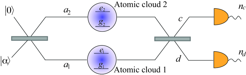
Figure 1: QND entangling scheme: An initial coherent light pulse $|\alpha\rangle$ is used to entangle two atomic clouds via the ac stark shift arranged in Mach-Zehnder interferometer configuration. Each of the beamsplitters are 50/50. The detection of photon outcomes $n_{c},n_{d}$ collapses the state of atomic clouds into entangled states.

II.1 Definitions

First consider the states of the atomic gas clouds (see Fig. 1). We consider each atom within the ensembles to be occupied by one of two internal states. For example, the states may be two hyperfine ground states of an atom (e.g. $F=1,m=-1$ and $F=2,m=+1$ for ⁸⁷Rb). The motional degrees of freedom of the atom are decoupled from the spin and may be neglected. In the case of a BEC, we may define bosonic annihilation operators $e_{j},g_{j}$ for the two internal states respectively, and $j\in\{1,2\}$ label the two atomic ensembles Byrnes and Ilo-Okeke (2021). For a collection of $N$ atoms in each BEC, the initial state of the atomic cloud can be described by

$$|\psi\rangle=\sum_{k_{1},k_{2}=0}^{N}\psi_{k_{1}k_{2}}|k_{1},k_{2}\rangle,$$ (1)

where we have defined the Fock states on the $j$th atomic ensemble as

$$|k\rangle=\frac{(e_{j}^{\dagger})^{k}(g_{j}^{\dagger})^{N-k}}{\sqrt{k!(N-k)!}}|\text{vac}\rangle,$$ (2)

and

$$|k_{1},k_{2}\rangle=|k_{1}\rangle\otimes|k_{1}\rangle.$$ (3)

Here the Fock states obey $\langle k|k^{\prime}\rangle=\delta_{kk^{\prime}}$ and the coefficients $\sum_{k_{1},k_{2}}|\psi_{k_{1}k_{2}}|^{2}=1$ are normalized.

For uncondensed thermal atomic gases, in general there are $2^{N}$ possible spin configurations per ensemble, instead of the $N+1$ states as defined in (2). However, if the initial state and all applied Hamiltonians are completely symmetric under particle interchange on a single ensemble, there is a mathematical equivalence between the BEC description and the thermal ensemble Byrnes and Ilo-Okeke (2021). Since we will work in the completely symmetric subspace, our results will be equally valid for the thermal atomic case, despite using the bosonic notation.

The collective spin operators on the $j$th ensemble are defined by

$$S^{x}_{j} =e_{j}^{\dagger}g_{j}+e_{j}^{\dagger}g_{j}$$

$$S^{y}_{j} =-ie_{j}^{\dagger}g_{j}+ig_{j}^{\dagger}e_{j}$$

$$S^{z}_{j} =e_{j}^{\dagger}e_{j}-g_{j}^{\dagger}g_{j},$$ (4)

obeying commutation relations $[S^{j},S^{k}]=2i\epsilon_{jkl}S^{l}$, where $\epsilon_{jkl}$ is the completely anti-symmetric Levi-Civita tensor. Spin coherent states, which are completely polarized spin configurations with Bloch sphere angles $\theta,\phi$ are defined as

$$|\theta,\phi\rangle\rangle=\frac{1}{\sqrt{N!}}\left(e^{\dagger}\cos\frac{\theta}{2}+g^{\dagger}e^{i\phi}\sin\frac{\theta}{2}\right)^{N}|\text{vac}\rangle.$$ (5)

Expanding the spin coherent state we may equally write this in terms of Fock states

$$|\theta,\phi\rangle\rangle=\sum_{k=0}^{N}\sqrt{N\choose k}e^{i(N-k)\phi}\cos^{k}\frac{\theta}{2}\sin^{N-k}\frac{\theta}{2}|k\rangle.$$ (6)

II.2 QND entangled wavefunction

The QND entangling scheme is shown in Fig. 1. Here, coherent light is arranged in a Mach-Zehnder configuration and the two atomic gases are placed in each arm of the interferometer. Preparing the atoms in the initial state (1), the light interacts with the atomic spins via the QND Hamiltonian Ilo-Okeke and Byrnes (2014),

$$H=\frac{\hbar\Omega}{2}(S^{z}_{1}-S^{z}_{2})(a^{\dagger}_{1}a_{1}-a^{\dagger}_{2}a_{2}),$$ (7)

where $a_{1},a_{2}$ denote the bosonic annihilation operators of the light in the two arms of the interferometer. After interacting with the atoms, the two modes are interfered via the second beam splitter and the photons are detected.

The above sequence modulates the quantum state of the atoms due to the atom-light entanglement that is generated by the QND interaction. This can be evaluated exactly due to the diagonal form of (7). We refer the reader to Ref. Aristizabal-Zuluaga et al. (2021) for further details and present only the final result. The final unnormalized state after detection of $n_{c},n_{d}$ photons in modes $c,d$ respectively is

$$|\widetilde{\psi}_{n_{c},n_{d}}(\tau)\rangle=\sum_{k_{1},k_{2}=0}^{N}\psi_{k_{1},k_{2}}C_{n_{c},n_{d}}[(k_{1}-k_{2})\tau]|k_{1},k_{2}\rangle,$$ (8)

where we defined the function

$$C_{n_{c},n_{d}}(\chi)=\frac{\alpha^{n_{c}+n_{d}}e^{-|\alpha|^{2}/2}}{\sqrt{n_{c}!n_{d}!}}\cos^{n_{c}}(\chi)\sin^{n_{d}}(\chi).$$ (9)

Here, $\alpha$ is the amplitude of the coherent light entering the first beamsplitter in Fig. 1 and $\tau=\Omega t$. The probability of obtaining a photonic measurement outcome $n_{c},n_{d}$ is

$$p_{n_{c},n_{d}}(\tau) =\langle\widetilde{\psi}_{n_{c},n_{d}}(\tau)|\widetilde{\psi}_{n_{c},n_{d}}(\tau)\rangle$$

$$=\sum_{k_{1},k_{2}=0}^{N}|\psi_{k_{1}k_{2}}C_{n_{c},n_{d}}[(k_{1}-k_{2})\tau]|^{2}.$$ (10)

We note that the $C$-functions are normalized according to

$$\sum_{n_{c},n_{d}=0}^{\infty}|C_{n_{c},n_{d}}(\chi)|^{2}=1.$$ (11)

The most likely photon number counting outcomes are centered around

$$n_{c}+n_{d}\approx|\alpha|^{2},$$ (12)

since the input coherent state has an average photon number of $|\alpha|^{2}$ and the remaining operations are photon number conserving.

The $C$-functions can be approximated for bright coherent light regime $|\alpha|\gg 1$ as

$$C_{n_{c}n_{d}}(\chi)\approx \frac{\alpha^{n_{c}+n_{d}}e^{-|\alpha|^{2}/2}}{\sqrt{(n_{c}+n_{d})!}}\frac{\text{sgn}(\cos^{n_{c}}(\chi)\sin^{n_{d}}(\chi))}{(\frac{\pi}{2}(n_{c}+n_{d})\sin^{2}2\chi)^{1/4}}$$

$$\times \exp\Big{[}-\frac{(n_{c}+n_{d})}{\sin^{2}2\chi}\big{(}\sin^{2}\chi-\frac{n_{d}}{n_{c}+n_{d}}\big{)}^{2}\Big{]},$$ (13)

for $n_{d}>0$. In the case of $n_{d}=0$, the $C$-function is better approximated as

$$C_{n_{c}n_{d}=0}(\chi)\approx\frac{\alpha^{n_{c}}e^{-|\alpha|^{2}/2}}{\sqrt{n_{c}!}}e^{-\frac{n_{c}}{2}\sin^{2}\chi}.$$ (14)

II.3 Example

To see how entanglement is generated by the QND scheme, let us choose an initial state for the atoms that is polarized in the $S^{x}$-direction

$$|\psi_{0}\rangle =|\frac{\pi}{2},0\rangle\rangle|\frac{\pi}{2},0\rangle\rangle$$

$$=\frac{1}{2^{N}}\sum_{k_{1},k_{2}=0}^{N}\sqrt{{N\choose k_{1}}{N\choose k_{2}}}|k_{1},k_{2}\rangle.$$ (15)

Now consider the $n_{c}\sim|\alpha|^{2},n_{d}=0$ photonic measurement outcome, which is a high probability result for short interaction times $\tau\sim 1/N$. Using the approximation (14) in (8) with $\sin\chi\approx\chi$, we obtain

$$|\widetilde{\psi}_{n_{c},n_{d}}(\tau)\rangle\propto\sum_{k_{1},k_{2}=0}^{N}\sqrt{{N\choose k_{1}}{N\choose k_{2}}}e^{-\frac{n_{c}\tau^{2}}{2}(k_{1}-k_{2})^{2}}|k_{1},k_{2}\rangle.$$ (16)

In the regime $n_{c}\tau^{2}\approx|\alpha\tau|^{2}>1$, the Gaussian factor suppresses terms except for $k_{1}=k_{2}$. This takes the form of an entangled state Aristizabal-Zuluaga et al. (2021); Kitzinger et al. (2020).

III Quantum measurement theory for QND induced entanglement

In quantum mechanics, a measurement is represented by a positive operator-valued measure (POVM) Nielsen and Chuang (2011), of which projective measurements are a special case. The QND entangling procedure may be viewed as a particular way of measuring the atomic states such that it collapses the state onto an entangled state. In this section, we introduce a POVM based theory of QND measurements, and its associated relations to connect the photonic readouts to particular projection operators.

III.1 QND POVM operators

According to the QND entangling protocol described in the previous section, the initial wave function (1) is modulated by an extra factor of $C_{n_{c},n_{d}}[(k_{1}-k_{2})\tau]$ and the final state becomes (8). An efficient way of summarizing this procedure is to define the measurement operator

$$M_{n_{c}n_{d}}(\tau)=\sum_{k_{1},k_{2}=0}C_{n_{c},n_{d}}[(k_{1}-k_{2})\tau]|k_{1},k_{2}\rangle\langle k_{1},k_{2}|.$$ (17)

According to the theory of quantum measurements, the resulting state after the measurement is

$$|\widetilde{\psi}_{n_{c}n_{d}}(\tau)\rangle=M_{n_{c}n_{d}}(\tau)|\psi\rangle$$ (18)

and the probability of this outcome is

$$p_{n_{c}n_{d}}(\tau)=\langle\psi|M_{n_{c}n_{d}}^{\dagger}(\tau)M_{n_{c}n_{d}}(\tau)|\psi\rangle$$ (19)

in agreement with (8) and (10) respectively. Since $M_{n_{c}n_{d}}^{\dagger}(\tau)M_{n_{c}n_{d}}(\tau)$ is a positive operator and we can evaluate

$$\sum_{n_{c},n_{d}}M^{\dagger}_{n_{c}n_{d}}(\tau)M_{n_{c},n_{d}}(\tau)=I$$ (20)

due to the relation (11), we may say that $M_{n_{c}n_{d}}(\tau)$ satisfies the definition of being a POVM.

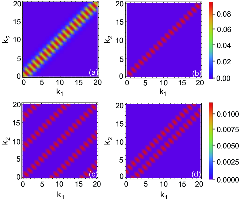
Figure 2: Plot of $C_{n_{c},n_{d}}[(k_{1}-k_{2})\tau]$ in (9) with different Fock state pairs for different photon detection outcomes and interaction times. Interaction times are (a) $t=\frac{\pi}{8N}$, (b) $t=\frac{\pi}{2N}$, (c) $t=\frac{\pi}{8}$, (d) $t=\frac{\pi}{2N}$. The measurement outcomes are (a)(b)(c) $n_{c}=|\alpha|^{2},n_{d}=0$, (d) $n_{c}=|\alpha|^{2}-\alpha,n_{d}=\alpha$. For all calculations, number of atoms per BEC is $N=30$ and $\alpha=50$. The scale for (a)-(c) are the same and shown next to (b). The scale for (d) is shown separately and is shown adjacent to the figure.

The type of the measurement induced by $M_{n_{c}n_{d}}(\tau)$ depends greatly upon the interaction time $\tau$ and the outcomes $n_{c},n_{d}$. First let us look at the effect of the interaction time $\tau$. In Fig. 2, we plot the modulating function $C_{n_{c},n_{d}}[(k_{1}-k_{2})\tau]$ for various photon detection outcomes $n_{c},n_{d}$ and interaction times $\tau$. First setting $n_{d}=0$ and comparing $\tau=\pi/8N,\pi/2N$ (Figs. 2(a)(b)) we see that for shorter times than $\tau=\pi/2N$ the function along the diagonal $k_{1}=k_{2}$ is broadened. For interaction times longer than $\tau=\pi/2N$, additional diagonal lines occur (Fig. 2(c)) according to the location of the peak of the Gaussian in (13)

$$\sin^{2}[(k_{1}-k_{2})\tau]=\frac{n_{d}}{n_{c}+n_{d}}.$$ (21)

For measurement outcomes detecting $n_{d}>0$ as in Fig. 2(d), we see the correlations are offset following the relation (21).

To explicitly see the effect of the various $n_{c},n_{d}$ outcomes, we plot the probability of the measurement outcome

$$p_{n_{c}n_{d}}(\tau) =\langle k,k+\Delta|M_{n_{c}n_{d}}^{\dagger}(\tau)M_{n_{c}n_{d}}(\tau)|k,k+\Delta\rangle$$

$$=|C_{n_{c},n_{d}}(\Delta\tau)|^{2}.$$ (22)

This gives the probability of various $n_{c},n_{d}$ outcomes for a state that differs in Fock state by $\Delta=k_{2}-k_{1}$. In Fig. 3 we see a probability curve that is centered around (21). For a time $t=\pi/2N$, there is a one-to-one relation between the measurement readout $n_{c},n_{d}$ and the magnitude of the Fock number difference $|\Delta|$ (Fig. 3(a)). At this time, the two Fock state differences that have a high probability are

$$\Delta =\pm\frac{1}{\tau}\sin^{-1}\sqrt{\frac{n_{c}}{n_{c}+n_{d}}}.$$ (23)

For longer times, the relationship is no longer one-to-one (Fig. 3(b)), and corresponds to the multiple diagonal lines seen in Fig. 2(c). In order to have a sharply defined projections without additional peaks in $\Delta$, we henceforth consider the time $\tau=\pi/2N$.

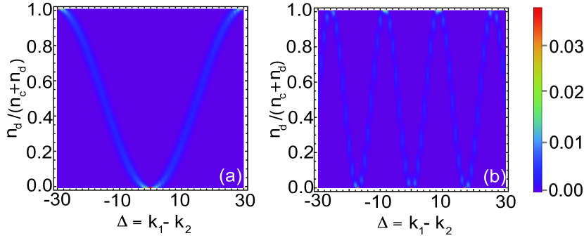
Figure 3: Relation of various photon detection outcomes $n_{c},n_{d}$ with offset in Fock states $\Delta=k_{1}-k_{2}$ for (a) $\tau=\frac{\pi}{2N}$, (b) $\tau=\frac{1}{\sqrt{N}}$ for $N=30,\alpha=10$.

III.2 QND projection operators

In the limit that the intensity of coherent light $|\alpha|^{2}$ is very bright such that $|\alpha\tau|^{2}>1$, the Gaussian function in (13) is sharply defined and strongly suppresses values of $k_{1}-k_{2}$ away from (21). In this limit, when two such measurements are made in succession, the net result is a projection operator. Taking the interaction time $\tau=\pi/2N$, there are two values of $k_{1}-k_{2}$ where the projections occur (Fig. 2(d)), as given by (23). We may then approximate the POVM according to

$$M_{n_{c}n_{d}}(\tau=\frac{\pi}{2N})\approx\mathcal{M}_{\Delta}\hskip 28.45274pt(|\alpha\tau|^{2}\gg 1)$$ (24)

where the $\Delta$ and $n_{c},n_{d}$ are related according to (23), and we define

$$\mathcal{M}_{\Delta}= \frac{1}{2^{\delta_{\Delta}}}\Big{(}\sum_{k=0}^{N-\Delta}|k,k+\Delta\rangle\langle k,k+\Delta|$$

$$\pm\sum_{k^{\prime}=\Delta}^{N}|k^{\prime},k^{\prime}-\Delta\rangle\langle k^{\prime},k^{\prime}-\Delta|\Big{)}.$$

A double sequence of such POVMs then gives the projection operator

$$P_{\Delta}= \mathcal{M}_{\Delta}\mathcal{M}_{\Delta}$$

$$= \frac{1}{2^{\delta_{\Delta}}}\Big{(}\sum_{k=0}^{N-\Delta}|k,k+\Delta\rangle\langle k,k+\Delta|$$

$$+\sum_{k^{\prime}=\Delta}^{N}|k^{\prime},k^{\prime}-\Delta\rangle\langle k^{\prime},k^{\prime}-\Delta|\Big{)}.$$ (25)

Here $\delta_{\Delta}$ is the Kronecker delta which is 1 if $\Delta=0$ and 0 otherwise.

The above projection operators are defined with respect to Fock states that are in the $S^{z}$ basis. We may equally define the Fock states in a different basis Byrnes and Ilo-Okeke (2021)

$$|k\rangle^{(\theta,\phi)}={\cal U}(\theta,\phi)|k\rangle^{(z)}$$ (26)

where

$${\cal U}(\theta,\phi)=e^{-i(S^{z}_{1}+S^{z}_{2})\phi/2}e^{-i(S^{y}_{1}+S^{y}_{2})\theta/2}$$ (27)

and $|k\rangle^{(z)}$ are the same Fock states as defined in (2). The projection operators may then be defined with respect to Fock states in a different basis

$$P_{\Delta}^{(\theta,\phi)}={\cal U}(\theta,\phi)P_{\Delta}^{(z)}{\cal U}^{\dagger}(\theta,\phi)$$ (28)

where $P_{\Delta}^{(z)}$ is the same projector as in (25), but we explicitly specified the basis with the ^(z) label. For the case that $\theta=\pi/2$ and $\phi=0$, the unitary rotation transforms the $S^{z}$ eigenstates to $S^{x}$ eigenstates and we define

$$P_{\Delta}^{(x)}={\cal U}(\frac{\pi}{2},0)P_{\Delta}^{(z)}{\cal U}^{\dagger}(\frac{\pi}{2},0).$$ (29)

III.3 Properties of projection operators

Here we list the properties of projection operators (28). These also apply to the specific cases (25) and (29).

1. The projection operators are idempotent and orthogonal

   $$P_{\Delta}^{(\theta,\phi)}P_{\Delta^{\prime}}^{(\theta,\phi)}=\delta_{\Delta\Delta^{\prime}}P_{\Delta}^{(\theta,\phi)}.$$ (30)

2. Projection operators are Hermitian

   $$(P^{(\theta,\phi)}_{\Delta})^{\dagger}=P^{(\theta,\phi)}_{\Delta}.$$ (31)

3. Projection operators are complete

   $$\sum_{\Delta}(P^{(\theta,\phi)}_{\Delta})^{\dagger}P^{(\theta,\phi)}_{\Delta}=\sum_{\Delta}P^{(\theta,\phi)}_{\Delta}=I.$$ (32)

4. The eigenvalues and eigenvectors of projection operators are

   $$P_{\Delta}^{(\theta,\phi)}|k,k+\Delta^{\prime}\rangle^{(\theta,\phi)}=\delta_{\Delta\Delta^{\prime}}|k,k+\Delta^{\prime}\rangle^{(\theta,\phi)}.$$ (33)

The proofs of these properties are straightforward and can be verified by substituting the definitions.

III.4 Example

We show that the projection operator can generate entanglement between the two atomic ensembles by applying it to the initial state (15). For example, for the outcome $\Delta=0$ we have

$$P_{\Delta=0}^{(z)}|\psi_{0}\rangle=\frac{1}{2^{N}}\sum_{k=0}^{N}{N\choose k}|k,k\rangle.$$ (34)

Similarly to that obtained in Sec. II.3, we obtain an entangled state between the two BECs.

We point out that the entanglement generation depends upon the preparation of a suitable initial state. From (33) it is evident that the projection operator applied to a product state of two Fock states leaves it unchanged. Since a product state does not possess entanglement between the BECs, the operation does not produce entanglement in this case. In this sense, a single QND measurement should not be considered an equivalent of Bell measurement, for which any initial state and measurement outcome results in an entangled state. It is better described as a projective operation which can result in an entangled state for suitable initial states. In the next sections we show how a sequence of projections can drive an arbitrary initial state into an entangled state.

IV Sequential QND projections: pure state analysis

In Ref. Aristizabal-Zuluaga et al. (2021) a two-pulse scheme for improved entanglement generation was analyzed. In the scheme, first the initial state (15) is prepared, and a QND measurement is performed, to yield a state similar to (34). Then a unitary rotation $e^{iS^{x}_{1}\pi/4}e^{-iS^{x}_{2}\pi/4}$ was performed and the QND measurement was repeated. This was found to produce a more strongly entangled state than using only a single QND measurement. Such a sequence of pulses have been used experimentally in several studies to enhance the entanglement in single atomic ensembles Behbood et al. (2013a, b); Behbood et al. (2014); Vasilakis et al. (2015). We show in this section that the technique is equally applicable in the two-ensemble case, and develop a theory to evaluate the result of multiple projections.

IV.1 Multiple QND measurements

First let us define the multiple QND measurement scheme in terms of the formalism we have introduced so far. We work in the regime $|\alpha\tau|^{2}>1$ such that the QND measurements can be described using the projection operators introduced in Sec. III.2. Let us define a particular QND projection sequence as

$$T_{\vec{\Delta}_{2L}} =P_{\Delta^{x}_{L}}^{(x)}P_{\Delta^{z}_{L}}^{(z)}\dots P_{\Delta^{x}_{2}}^{(x)}P_{\Delta^{z}_{2}}^{(z)}P_{\Delta^{x}_{1}}^{(x)}P_{\Delta^{z}_{1}}^{(z)}$$

$$=\prod_{l=1}^{L}\Big{[}P_{\Delta^{x}_{l}}^{(x)}P_{\Delta^{z}_{l}}^{(z)}\Big{]}.$$ (35)

where the projections in the $z$- and $x$-basis are defined in (25) and (29) respectively. In the product operator, we take the convention that the order of the projectors is arranged from right to left, for labels running from the lower index to the upper index. Each projection is made in an alternating basis switching between $z$ and $x$. The sequence consists of $L$ repetitions of projections in the $z$ and $x$ basis. We take the convention that a sequence always starts with a projection in the $z$-basis. Equation (35) is an example where there are an even number of projections (a total of $2L$ projections) in total. Thus in this case the last projector will be in the $x$-basis. The outcomes are specified by an ordered list

$$\vec{\Delta}_{2L}=(\Delta_{1}^{z},\Delta_{1}^{x},\Delta_{2}^{z},\Delta_{2}^{x},\dots,\Delta_{L}^{z},\Delta_{L}^{x}).$$ (36)

where the subscript $2L$ shows the number of projections that are made. Physically, these can be interpreted as the random outcomes associated with a particular projection sequence.

For an odd number of projections, we have instead

$$T_{\vec{\Delta}_{2L+1}} =P_{\Delta^{z}_{L+1}}^{(z)}P_{\Delta^{x}_{L}}^{(x)}P_{\Delta^{z}_{L}}^{(z)}\dots P_{\Delta^{x}_{2}}^{(x)}P_{\Delta^{z}_{2}}^{(z)}P_{\Delta^{x}_{1}}^{(x)}P_{\Delta^{z}_{1}}^{(z)}$$

$$=P_{\Delta^{z}_{L+1}}^{(z)}\prod_{l=1}^{L}\Big{[}P_{\Delta^{x}_{l}}^{(x)}P_{\Delta^{z}_{l}}^{(z)}\Big{]}.$$ (37)

Here a particular sequence is specified by $2L+1$ parameters

$$\vec{\Delta}_{2L+1}=(\Delta_{1}^{z},\Delta_{1}^{x},\Delta_{2}^{z},\Delta_{2}^{x},\dots,\Delta_{L}^{z},\Delta_{L}^{x},\Delta_{L+1}^{z}).$$ (38)

We shall see that the parity of the number of projections (i.e. whether it is even or odd) will make a large difference to the final state. When discussing a property without any parity dependence, we will drop the subscript on $\vec{\Delta}$ for brevity.

Starting from an initial state $|\psi_{0}\rangle$, after a particular projection sequence we obtain an unnormalized state (denoted by the tilde)

$$|\tilde{\psi}_{\vec{\Delta}}\rangle =T_{\vec{\Delta}}|\psi_{0}\rangle.$$ (39)

The probability of this particular outcome labeled by $\vec{\Delta}$ occurring is

$$p_{\vec{\Delta}}=\langle\tilde{\psi}_{\vec{\Delta}}|\tilde{\psi}_{\vec{\Delta}}\rangle,$$ (40)

where the probabilities satisfy

$$\sum_{\vec{\Delta}}p_{\vec{\Delta}}\equiv\sum_{\Delta_{1}^{z}}\sum_{\Delta_{1}^{x}}\dots\sum_{\Delta_{L+1}^{z}}p_{\vec{\Delta}}=1.$$ (41)

We may visualize the sequence of projections as shown in Fig. 4. Each projection occurs randomly and yields in general a different state. Successive projections yield new states that depend upon the past projection outcomes.

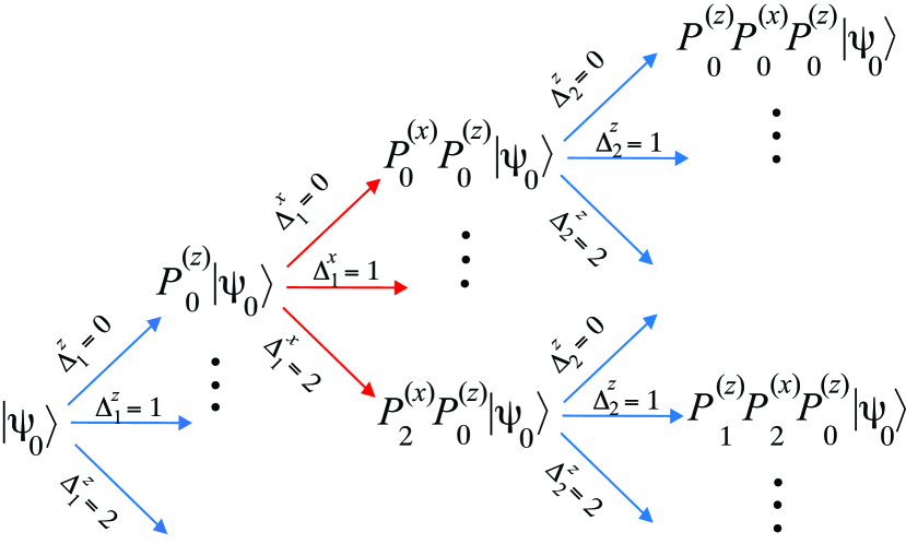
Figure 4: Tree diagram corresponding to the multiple QND projection sequence $T_{\vec{\Delta}}$. Each branch of the tree corresponds to different projection outcomes labelled by (38). The probability of a particular outcome is given by (40).

We note that the sequence of projection operators $T_{\vec{\Delta}}$ is not itself a projection operator. Specifically, the property of idempotence and orthogonality (30) does not hold. They are however complete and satisfy

$$\sum_{\vec{\Delta}}T_{\vec{\Delta}}^{\dagger}T_{\vec{\Delta}}=\sum_{\vec{\Delta}}T_{\vec{\Delta}}=I,$$ (42)

which may be used to show (41).

IV.2 Example: convergence to maximally entangled state

To see the effect of the multiple QND projections, it is illustrative to see a simple example. Let us consider the particular outcome sequence with an odd number of projections

$$\vec{\Delta}_{2L+1}=(0,0,\dots,0).$$ (43)

The final state in this case is

$$|\tilde{\psi}_{\vec{\Delta}_{2L+1}}\rangle=P_{0}^{(z)}\Big{(}P_{0}^{(x)}P_{0}^{(z)}\Big{)}^{L}|\psi_{0}\rangle.$$ (44)

The effect of the projector $P_{0}^{(z)}$ is to remove all elements from the wavefunction except $k_{1}=k_{2}$ in (1). Hence after each projector $P_{0}^{(z)}$ the state is guaranteed to be in a state of the form

$$\sum_{k=0}^{N}\psi_{kk}|k,k\rangle.$$ (45)

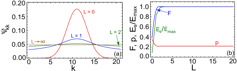
Figure 5: Analysis of multiple QND projections: (a)The resulting wavefunction after multiple QND projections of the form (39). The $z$-basis projected wavefunction of the form (45) is shown; (b) fidelity, entanglement and probability of the projected wavefunction for $N=20$. For both the figures we have considered $\vec{\Delta}_{2L+1}=(0,0,\dots,0)$.

The effect of multiple projections with $L$ can then be seen in Fig. 5(a), where we start in the initial state (15). We see that for $L=0$ the distribution takes a binomial form, as already seen in (34). The largest amplitude occurs at $k=N/2$. As $L$ is increased, the state gradually flattens out. This can also be seen in terms of the spin correlations. In Fig. 6 we show the probability of the projected state after multiple QND measurements in various spin bases i.e. $|k\rangle^{(x)}$, $|k\rangle^{(y)}$ and $|k\rangle^{(z)}$ which are eigenstates of the spin operators $S^{x}$, $S^{y}$ and $S^{z}$ respectively. The probability of the measurement outcomes $k_{1},k_{2}$ for various Fock states is defined as

$$p_{l_{1}l_{2}}=\frac{|\langle\tilde{\psi}_{\vec{\Delta}_{2L+1}}|\Big{(}|k\rangle^{(l_{1})}\otimes|k\rangle^{(l_{2})}\Big{)}|^{2}}{\langle\tilde{\psi}_{\vec{\Delta}_{2L+1}}|\tilde{\psi}_{\vec{\Delta}_{2L+1}}\rangle},$$ (46)

where the final projected state is used (39). We see that the spin correlations are improved and become more sharply defined, with correlations in the $S^{x},S^{z}$ variables and anticorrelations in $S^{y}$.

After a larger number of QND measurement rounds, these spin correlations converge to that of a spin-EPR state (47) (see Fig. 6(c)). The improvement in the spin correlations is one of the reasons such a measurement sequence would be performed in practice. The state converges to the maximally entangled state

$$|\text{EPR}_{+}\rangle=\frac{1}{\sqrt{N+1}}\sum_{k=0}^{N}|k,k\rangle^{(z)}.$$ (47)

This state has basis invariant properties analogous to Bell states, and can be written equivalently as Kitzinger et al. (2020)

$$|\text{EPR}_{+}\rangle=\frac{1}{\sqrt{N+1}}\sum_{k=0}^{N}|k,k\rangle^{(x)}.$$ (48)

This state is an eigenstate of both the $P_{0}^{(z)}$ and $P_{0}^{(x)}$ projectors with eigenvalue 1, hence for large $L$ the state converges to the above state. In Fig. 5(b) we show the fidelity of the state

$$F=\frac{|\langle\text{EPR}_{+}|\tilde{\psi}_{\vec{\Delta}_{2L+1}}\rangle|^{2}}{\langle\tilde{\psi}_{\vec{\Delta}_{2L+1}}|\tilde{\psi}_{\vec{\Delta}_{2L+1}}\rangle}$$ (49)

as a function of $L$. We see that the fidelity approaches 1 rapidly. The probability of obtaining the outcome (40) approaches a value of $\approx 0.22$ that is for a single projection outcome. We note that for the outcome (43), the state converges to the state (47) regardless of the initial state. The convergence properties will however be different for different initial states.

Figure 6: Spin correlations after multiple QND projections of the form (39), measured in various bases according to (46). The number of QND measurement rounds is (a) $L=1$; (b) $L=2$; (c) $L=6$. The number of atoms in each ensemble is $N=15$ and the measurement outcome is taken as $\vec{\Delta}_{2L+1}=(0,0,\dots,0)$.

The state (47) is a maximally entangled state, and accordingly we may confirm the convergence of entanglement (Fig. 5(b)). The entanglement can be quantified by the von Neumann entropy, defined as

$$E(\rho)=-\text{Tr}(\rho\log_{2}\rho).$$ (50)

where the reduced density matrix on BEC 1 is

$$\rho=Tr_{2}(|\tilde{\psi}_{\vec{\Delta}_{2L+1}}\rangle\langle\tilde{\psi}_{\vec{\Delta}_{2L+1}}|)$$ (51)

In Fig. 5(b) we have normalized it with maximum entanglement between two BECs $E_{\text{max}}=\log_{2}(N+1)$. The entanglement increases and saturates at maximum value once the state has a high fidelity with the state (47).

IV.3 Singular value decomposition of two projectors

The example in the previous section illustrates the general behavior of multiple QND projections. The basic behavior is that after a number of QND measurements, the state converges to a fixed state. This was a relatively simple example, where some known properties of the states could be used to deduce the final state. We now examine the more general case for an arbitrary $\vec{\Delta}$.

The following key mathematical result greatly simplifies the subsequent analysis:

Lemma 1.

Consider a sequence of two projections

$$T_{\Delta^{z}\Delta^{x}}=P_{\Delta^{x}}^{(x)}P_{\Delta^{z}}^{(z)}$$ (52)

as defined in (35). Its singular value decomposition can be written

$$T_{\Delta^{z}\Delta^{x}}=U\Lambda_{\Delta^{z}\Delta^{x}}V^{\dagger}$$ (53)

where $U,V$ are unitary matrices that are independent of $\Delta^{z},\Delta^{x}$, and $\Lambda_{\Delta^{z},\Delta^{x}}$ is a diagonal matrix up to a permutation of rows and columns, i.e. a matrix with only one non-zero element in each row and column.

Proof.

The full proof is given in Appendix A. Here we provide the main steps of the proof. First define the Hermitian matrix

$$R_{\Delta^{z}\Delta^{x}} \equiv T_{\Delta^{z}\Delta^{x}}^{\dagger}T_{\Delta^{z}\Delta^{x}}$$ (54)

$$=P_{\Delta^{z}}^{(z)}P_{\Delta^{x}}^{(x)}P_{\Delta^{z}}^{(z)}$$ (55)

From Appendix A, it follows that for arbitrary choices of the index $\Delta^{z},\Delta^{x}$ we have

$$[R_{\Delta^{z}\Delta^{x}},R_{{\Delta^{z}}^{\prime}{\Delta^{x}}^{\prime}}]=0.$$ (56)

For any two commuting Hermitian matrices, it is possible to write down a common unitary transformation that diagonalizes both the operators. Since all $R$’s mutually commute, there is a common unitary transformation for all the $R$’s. Hence

$$R_{\Delta^{z}\Delta^{x}}=VD_{\Delta^{z}\Delta^{x}}V^{\dagger},$$ (57)

where $D$ is a diagonal matrix. Substituting (53) in (54) we have

$$R_{\Delta^{z}\Delta^{x}}=V\Lambda_{\Delta^{z}\Delta^{x}}\Lambda_{\Delta^{z}\Delta^{x}}^{\dagger}V^{\dagger}.$$ (58)

Proving (56) for all possible $\Delta^{z}$ and $\Delta^{x}$ demonstrates that a common set of eigenvectors diagonalizes the Gram matrix $R_{\Delta^{z}\Delta^{x}}$, and the resultant eigenvector matrix therefore forms a consistent set of left singular vectors for $T_{\Delta^{z}\Delta^{x}}$. For the $U$ unitary matrix, the argument is identical except that one starts with the definition $R_{\Delta^{z}\Delta^{x}}=T_{\Delta^{z}\Delta^{x}}T_{\Delta^{z}\Delta^{x}}^{\dagger}$. ∎

An example of Lemma 1 is shown in Appendix B for illustration.

IV.4 Evaluation of multiple projectors

With the aid of Lemma 1, we may write a more general sequence of projections in simpler form.

Lemma 2.

The matrix product for a sequence of projections with an odd number of projectors as in (37) can be written

$$T_{\vec{\Delta}_{2L+1}} =V\left(\prod_{l=1}^{L}\Lambda_{\Delta_{l}^{x}\Delta_{l+1}^{z}}^{\dagger}\Lambda_{\Delta_{l}^{x}\Delta_{l}^{z}}\right)V^{\dagger},$$ (59)

and for an even number of projectors as in (35),

$$T_{\vec{\Delta}_{2L}} =U\Lambda_{\Delta_{L}^{x}\Delta_{L}^{z}}\left(\prod_{l=1}^{L-1}\Lambda_{\Delta_{l}^{x}\Delta_{l+1}^{z}}^{\dagger}\Lambda_{\Delta_{l}^{x}\Delta_{l}^{z}}\right)V^{\dagger},$$ (60)

for $L\geq 1$. Here the unitary matrices $U,V$ and the matrices $\Lambda_{\Delta_{l}^{x}\Delta_{l}^{z}}$ are the same as given in (53).

Proof.

Using the idempotence relation we can write (37) as

$$T_{\vec{\Delta}_{2L+1}} =\prod_{l=1}^{L}\Big{[}P_{\Delta^{z}_{l+1}}^{(z)}P_{\Delta^{x}_{l}}^{(x)}P_{\Delta^{x}_{l}}^{(x)}P_{\Delta^{z}_{l}}^{(z)}\Big{]}$$

$$=\prod_{l=1}^{L}T_{\Delta_{l+1}^{z}\Delta_{l}^{x}}^{\dagger}T_{\Delta_{l}^{z}\Delta_{l}^{x}}.$$ (61)

Substituting (53) into (61), the unitary rotations $U,V$ at all intermediate steps can be removed by $U^{\dagger}U=V^{\dagger}V=I$ since they are common for all $\Delta^{x},\Delta^{z}$. This yields (59). For (60), use (59) with $L\rightarrow L-1$ and apply (53) once. ∎

From Lemma 2, we see that in a sequence of projections, there is a particular basis where the evolution of the state becomes particularly simple. The $\Lambda$ matrices are diagonal up to a permutation of rows and columns, which means that the computation can be performed efficiently.

To illustrate this, let us now use Lemma 2 to determine the effect of applying the sequential projection for the particular case of an initial state in the $V$-basis

$$|\psi_{0}\rangle=|\bm{k}\rangle^{(V)}\equiv V|\bm{k}\rangle^{(z)},$$ (62)

where $|\bm{k}\rangle^{(z)}$ is defined in (3), and we have defined

$$\bm{k}=(k_{1},k_{2}).$$ (63)

Considering the case with an odd number of projectors first, apply (59) to (62). This results in the unnormalized state

$$T_{\vec{\Delta}_{2L+1}}|\bm{k}\rangle^{(V)}=V\left(\prod_{l=1}^{L}\Lambda_{\Delta_{l}^{x}\Delta_{l+1}^{z}}^{\dagger}\Lambda_{\Delta_{l}^{x}\Delta_{l}^{z}}\right)|\bm{k}\rangle^{(z)},$$ (64)

where we take the case with an odd number of projections. Since the matrix $\Lambda_{\Delta_{l}^{x}\Delta_{l}^{z}}$ is a permutation matrix up to some coefficients, the effect of each application of the matrix will be to change the labels $\bm{k}\rightarrow\bm{k}^{\prime}$, and adjust the normalization of the state. Let us define the permutation function associated with the matrix $\Lambda_{\Delta_{l}^{x}\Delta_{l}^{z}}$

$$\bm{k}^{\prime} =\pi_{\Delta^{x}\Delta^{z}}(\bm{k}).$$ (65)

For the matrix $\Lambda_{\Delta^{x}\Delta^{z}}^{\dagger}$, we have the inverse function

$$\bm{k} =\pi_{\Delta^{x}\Delta^{z}}^{-1}(\bm{k}^{\prime}).$$ (66)

Then for the $l$th pair of $\Lambda$ matrices in (64), the labels shift by

$$\bm{k}_{l}^{\prime} =\pi_{\Delta_{l}^{x}\Delta_{l}^{z}}(\bm{k}_{l})$$

$$\bm{k}_{l+1} =\pi^{-1}_{\Delta_{l}^{x}\Delta_{l+1}^{z}}(\bm{k}_{l}^{\prime}).$$ (67)

Here $\bm{k}_{l}^{\prime}$ are the state labels after application of $\Lambda_{\Delta_{l}^{x}\Delta_{l}^{z}}$ and $\bm{k}_{l+1}$ are the labels after the $\Lambda_{\Delta_{l}^{x}\Delta_{l+1}^{z}}^{\dagger}$. The initial state label is $\bm{k}_{1}=\bm{k}$ in (62). This is a recursive relation by which we can evaluate the final state indices.

The amplitude of (64) can be evaluated by defining the matrix element for this permutation as

$$a_{\Delta^{x}\Delta^{z}}(\bm{k})=\langle\bm{k}^{\prime}|\Lambda_{\Delta^{x}\Delta^{z}}|\bm{k}\rangle.$$ (68)

Application of each $\Lambda$ matrix gives a factor as given in (68). Thus the final coefficient is

$$A_{\vec{\Delta}_{2L+1}}(\bm{k})=\prod_{l=1}^{L}\Big{[}a_{\Delta^{x}_{l}\Delta^{z}_{l+1}}(\bm{k}_{l+1})a_{\Delta^{x}_{l}\Delta^{z}_{l}}(\bm{k}_{l})\Big{]},$$ (69)

and the $\bm{k}_{l}$ are evaluated by the recursion relation (67). We also define the result of $L$ rounds of recursion of the relation (67) as

$$r_{\vec{\Delta}_{2L+1}}(\bm{k})=\bm{k}_{L+1}.$$ (70)

Then (64) can be evaluated to give the unnormalized state

$$T_{\vec{\Delta}_{2L+1}}|\bm{k}\rangle^{(V)}=A_{\vec{\Delta}_{2L+1}}(\bm{k})|r_{\vec{\Delta}_{2L+1}}(\bm{k})\rangle^{(V)}.$$ (71)

For the case with an even number of projectors, we have

$$T_{\vec{\Delta}_{2L}}|\bm{k}\rangle^{(V)}=U\Lambda_{\Delta_{L}^{x}\Delta_{L}^{z}}\left(\prod_{l=1}^{L-1}\Lambda_{\Delta_{l}^{x}\Delta_{l+1}^{z}}^{\dagger}\Lambda_{\Delta_{l}^{x}\Delta_{l}^{z}}\right)|\bm{k}\rangle^{(z)},$$ (72)

using (60). The result of the recursion relation in this case is

$$r_{\vec{\Delta}_{2L}}(\bm{k})=\bm{k}_{L}^{\prime}.$$ (73)

and the coefficient is

$$A_{\vec{\Delta}_{2L}}(\bm{k})=a_{\Delta^{x}_{L}\Delta^{z}_{L}}(\bm{k}_{L})\prod_{l=1}^{L-1}\Big{[}a_{\Delta^{x}_{l}\Delta^{z}_{l+1}}(\bm{k}_{l+1})a_{\Delta^{x}_{l}\Delta^{z}_{l}}(\bm{k}_{l})\Big{]}.$$ (74)

The final unnormalized result in this case is

$$T_{\vec{\Delta}_{2L}}|\bm{k}\rangle^{(V)}=A_{\vec{\Delta}_{2L}}(\bm{k})|r_{\vec{\Delta}_{2L}}(\bm{k})\rangle^{(U)},$$ (75)

note that the final result is in the $U$-basis in this case because of the $U$ in (72).

For (71) and (75), the normalized state is simply $|r_{\vec{\Delta}}(\bm{k})\rangle^{(V)}$, unless $A_{\vec{\Delta}}(\bm{k})=0$ in which case the projection sequence is an outcome with zero probability.

We are now ready to state our first main result.

Theorem 1.

Applying a sequence of projections $T_{\vec{\Delta}}$ on an arbitrary initial state $|\phi\rangle$ results in the unnormalized state

$$T_{\vec{\Delta}_{2L+1}}|\phi\rangle=\sum_{\bm{k}}A_{\vec{\Delta}_{2L+1}}(\bm{k})\phi_{\bm{k}}^{(V)}|r_{\vec{\Delta}_{2L+1}}(\bm{k})\rangle^{(V)}$$ (76)

for an odd number of projectors as in (37) and

$$T_{\vec{\Delta}_{2L}}|\phi\rangle=\sum_{\bm{k}}A_{\vec{\Delta}_{2L}}(\bm{k})\phi_{\bm{k}}^{(V)}|r_{\vec{\Delta}_{2L}}(\bm{k})\rangle^{(U)}$$ (77)

for an even number of projectors as in (35). Here, $\phi_{\bm{k}}^{(V)}=\langle\bm{k}|V^{\dagger}|\phi\rangle$ is the amplitude of $|\phi\rangle$ in the $V$-basis, $L\geq 1$, $r_{\vec{\Delta}}(\bm{k})$ is the result of the recursion relation (70) and (73) and $A_{\vec{\Delta}}(\bm{k})$ is defined in (69) and (74).

Proof.

Inserting the resolution of the identity in the $V$-basis

$$T_{\vec{\Delta}}|\phi\rangle=T_{\vec{\Delta}}\sum_{\bm{k}}|\bm{k}\rangle^{(V)}\langle\bm{k}|^{(V)}|\phi\rangle$$ (78)

and using the results (71) and (75) give (76) and (77). ∎

It follows straightforwardly from (76) that the probability of a particular sequence of projections is given by

$$p_{\vec{\Delta}} =\langle\phi|T_{\vec{\Delta}}^{\dagger}T_{\vec{\Delta}}|\phi\rangle$$

$$=\sum_{\bm{k}}|A_{\vec{\Delta}}(\bm{k})\phi_{\bm{k}}^{(V)}|^{2}.$$ (79)

The states (76) and (77) can then be normalized by simply dividing by $\sqrt{p_{\vec{\Delta}}}$.

Equations (76) and (77) allows for a highly efficient way to evaluate the result of a sequence of projections. In words, the procedure is as follows. Given an arbitrary initial state $|\phi\rangle$, first expand the state in the $V$-basis, defined by (62). Then for each state labeled by $\bm{k}$, we can recursively apply (67) until we find $\bm{k}_{L}$. This results in obtaining the sequence of $\bm{k}_{l},\bm{k}_{l}^{\prime}$, from which the overall coefficient $A$ can be found through (69). Multiplying the coefficient by the associated term in the superposition gives (76). This procedure is far more efficient than evaluating $2L+1$ matrix multiplications directly, each with an overhead of $(N+1)^{6}$.

IV.5 Example: stochastic evolution

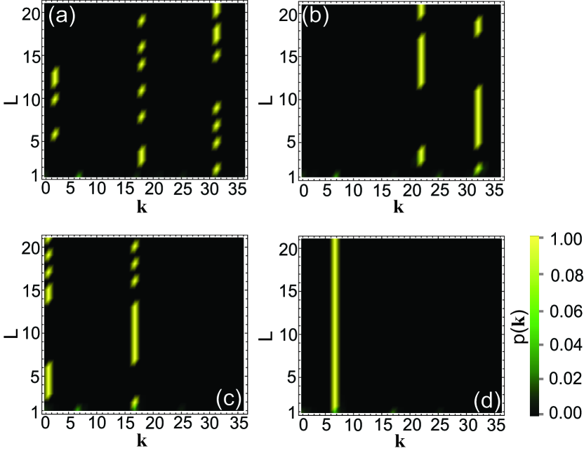
Figure 7: The probability distribution (80) of the quantum state after multiple QND projections (39) for the initial (a),(b) random state; (c),(d) $S_{x}$-polarized state. For all calculations number of atoms per BEC is taken as $N=5$. States are enumerated by $[\bm{k}]=k_{2}(N+1)+k_{1}$.

While (76) and (77) gives the general result for an arbitrary sequence of projections, for a typical sequence the resulting dynamics is often rather simple. Figure 7 shows the probability distribution of evolving a random initial state with the sequence of QND projections

$$p(\bm{k}) =\frac{|\langle\bm{k}|{{}^{(V)}}T_{\vec{\Delta}_{2L+1}}|\phi\rangle|^{2}}{p_{\vec{\Delta}_{2L+1}}},$$ (80)

where we consider an odd number of projections, such that the output state is in the $V$-basis. Here the measurement outcomes $\vec{\Delta}_{2L+1}$ are chosen randomly according to their measurement probabilities. We see that the state quickly becomes dominated by a single state in the $V$-basis $|\bm{k}\rangle^{(V)}$. Depending upon the measurement outcomes and the initial state, the state can remain fixed in a particular state (Fig. 7(d)), or jump randomly between several values (Fig. 7(a)-(c)). This depends upon the recursion relations (67). However, at any given step in the projection sequence, the state is typically in only only of the $|\bm{k}\rangle^{(V)}$ states.

The reason for this can be seen from (76). After a sequence of projections is applied, the state becomes modified by the factor $A_{\vec{\Delta}}(\bm{k})$. Since this is a product of matrix elements according to (69), depending upon the particular $\vec{\Delta}$ that occurs, one of the coefficients of $|\bm{k}\rangle^{(V)}$ becomes dominant, due to the exponential increase of a dominant factor. Similar results occur for an even number of projections, with the main difference being that the final state is in the $U$-basis.

We summarize the effect of multiple QND projections by the following basic rule-of-thumb: it collapses the state to one of the states in the $V$-basis for an odd number of projections, and one of the $U$-basis states for an even number of projections.

V Sequential QND projections: Mixed state analysis

In the previous section we considered the effect of applying a sequence of projections $T_{\vec{\Delta}}$ to a pure state. This results in a stochastic evolution of the state, as illustrated in Fig. 7. This corresponds to a single run of a particular experiment. It is also useful to analyze this in a statistical sense, where we deal with a probabilistic evolution of the state. The natural language for this are density matrices, and in this section we adapt the results of the previous section to the mixed state case.

V.1 Sequence of QND projections on a mixed state

Let us first generalize the results of the previous section to the case when the initial state is a mixed state with density matrix $\rho_{0}$. After performing a projection sequence the resulting unnormalized density matrix is

$$\tilde{\rho}_{\vec{\Delta}}=T_{\vec{\Delta}}\rho_{0}T_{\vec{\Delta}}^{\dagger}$$ (81)

occurring with probability

$$p_{\vec{\Delta}}=\text{Tr}(T_{\vec{\Delta}}^{\dagger}T_{\vec{\Delta}}\rho_{0}).$$ (82)

Instead of a single shot outcome as we considered in the last section, we now wish to obtain the average over many possible runs of the QND projector sequence. Let us here restrict ourselves to the case that there is an odd number of projections $\vec{\Delta}=\vec{\Delta}_{2L+1}$. Averaging over all possible outcomes the density matrix is

$$\rho^{(V)} =\sum_{\vec{\Delta}}(\prod_{l=1}^{L}\Lambda_{\Delta_{l}^{x}\Delta_{l+1}^{z}}^{\dagger}\Lambda_{\Delta_{l}^{x}\Delta_{l}^{z}})\rho^{(V)}_{0}(\prod_{l=1}^{L}\Lambda_{\Delta_{l}^{x}\Delta_{l+1}^{z}}^{\dagger}\Lambda_{\Delta_{l}^{x}\Delta_{l}^{z}})^{\dagger}$$ (83)

where we used (59) and we defined density matrices rotated into the $V$-basis as

$$\rho^{(V)}=V^{\dagger}\rho V.$$ (84)

Alternatively, we may use (76) to write

$$\rho^{(V)} =\sum_{\vec{\Delta}}\sum_{\bm{k}\bm{k}^{\prime}}A_{\vec{\Delta}}(\bm{k})A_{\vec{\Delta}}^{*}(\bm{k}^{\prime})\rho_{\bm{k}\bm{k}^{\prime}}^{(V)}|r_{\vec{\Delta}}(\bm{k})\rangle\langle r_{\vec{\Delta}}(\bm{k}^{\prime})|$$ (85)

where $\rho_{\bm{k}\bm{k}^{\prime}}^{(V)}=\langle\bm{k}|V^{\dagger}\rho_{0}V|\bm{k}^{\prime}\rangle$.

V.2 Example: probabilistic evolution

We now numerically evaluate the density matrix evolution to illustrate the effect of the multiple projections. To evaluate the density matrix, rather than the expressions (83) or (85) which contain a large number of summations over $\vec{\Delta}$, it is more efficient to evaluate the density matrices iteratively. Consider the application of an even number of projectors (35) and averaging over all outcomes we have

$$\rho_{l}^{\prime}=\sum_{\Delta^{z}_{1},\Delta^{x}_{1},\dots,\Delta^{x}_{l}}P^{(x)}_{\Delta^{x}_{l}}\dots P^{(z)}_{\Delta^{z}_{1}}\rho_{0}P^{(z)}_{\Delta^{x}_{1}}\dots P^{(x)}_{\Delta^{z}_{l}}.$$ (86)

For an odd number of projectors we have instead

$$\rho_{l+1}=\sum_{\Delta^{z}_{1},\Delta^{x}_{1},\dots,\Delta^{x}_{l},\Delta^{z}_{l+1}}P^{(z)}_{\Delta^{z}_{l+1}}P^{(x)}_{\Delta^{x}_{l}}\dots P^{(z)}_{\Delta^{z}_{1}}\rho_{0}P^{(z)}_{\Delta^{x}_{1}}\dots P^{(x)}_{\Delta^{z}_{l}}P^{(z)}_{\Delta^{z}_{l+1}}.$$ (87)

Then using property (30) of projection operators, we may relate the two density matrices by

$$\rho_{l+1}=\sum_{\Delta^{x},\Delta^{z}}T^{\dagger}_{\Delta^{z}\Delta^{x}}\rho_{l}^{\prime}T_{\Delta^{z}\Delta^{x}}.$$ (88)

Similarly, we may transform a density matrix with an odd number of projectors to an even one according to

$$\rho_{l}^{\prime}=\sum_{\Delta^{x},\Delta^{z}}T_{\Delta^{z}\Delta^{x}}\rho_{l}T^{\dagger}_{\Delta^{z}\Delta^{x}}.$$ (89)

Applying (53) we then find that

$${\rho_{l}^{\prime}}^{(U)} =\sum_{\Delta^{x},\Delta^{z}}\Lambda_{\Delta^{x}\Delta^{z}}^{\dagger}{\rho_{l}}^{(V)}\Lambda_{\Delta^{x}\Delta^{z}}$$ (90)

$$\rho_{l+1}^{(V)} =\sum_{\Delta^{x},\Delta^{z}}\Lambda_{\Delta^{x}\Delta^{z}}{\rho_{l}^{\prime}}^{(U)}\Lambda_{\Delta^{x}\Delta^{z}}^{\dagger}.$$ (91)

where we defined

$$\rho^{(U)}=U^{\dagger}\rho U.$$ (92)

From (90) and (91) we may find the resulting density matrix iteratively, by starting with the initial state $\rho_{0}=\rho_{1}$.

Figure 8 shows the density matrix evolution starting from two initial states, the state (15) and a random pure state. In Fig. 8(a)(b) we show the diagonal elements of the density matrix in the $V$-basis as a function of the total number of rounds of projections $L$. We see that in both cases the states rapidly converge to a fixed probability distribution. The particular distribution that is obtained, depends upon the initial state. The final convergent probability distributions correspond to the proportions of the state that would be obtained after many runs of the stochastic evolution as shown in Fig. 7.

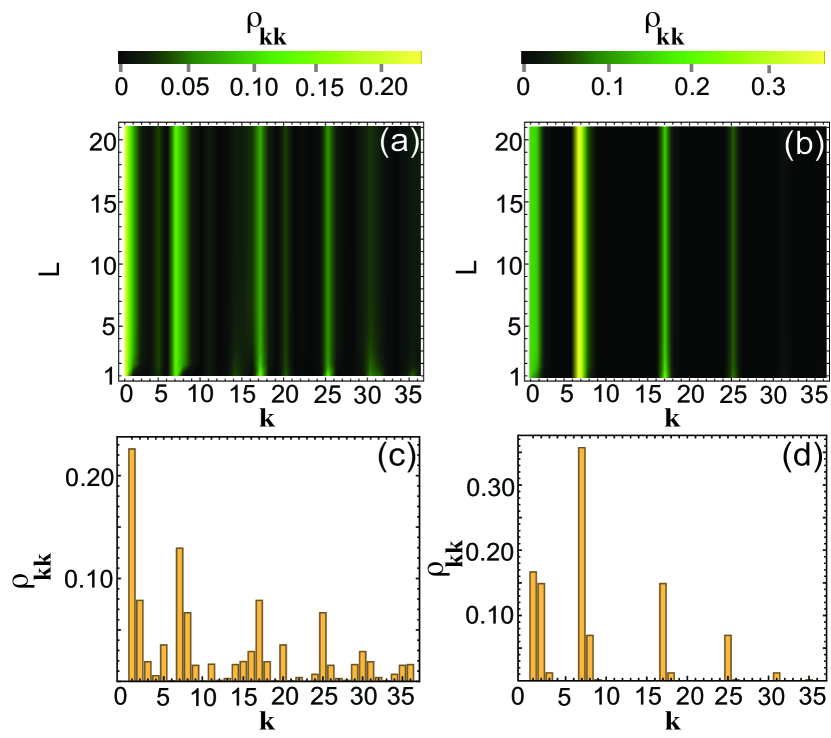
Figure 8: The probability distribution of the quantum mixed state after multiple QND projections (39) for the initial (a) random state; (b) $S_{x}$-polarized state. For all calculations number of atoms per BEC is taken as $N=5$. The corresponding probability bar charts are also shown at the bottom for each case. States are enumerated by $[\bm{k}]=k_{2}(N+1)+k_{1}$.

V.3 Steady-state distribution

We now show a method for finding the steady-state distribution of the density matrix, as illustrated in Fig. 8. After a large number of iterations $L$, the density matrix remains unchanged and reaches a fixed point. We again consider the case where there is an odd number of projectors, such as the final density matrix is in the $V$-basis. Combining (88) and (89), we then demand that

$$\rho=\sum_{\vec{\Delta}_{3}}T_{\vec{\Delta}_{3}}\rho T_{\vec{\Delta}_{3}}^{\dagger}$$ (93)

where $\vec{\Delta}_{3}=(\Delta^{z},\Delta^{x},{\Delta^{z}}^{\prime})$. Expanding the density matrix in the $V$-basis, we have

$$\rho=\sum_{\bm{k},\bm{k}^{\prime}}\rho_{\bm{k}\bm{k}^{\prime}}^{(V)}|\bm{k}\rangle^{(V)}\langle\bm{k}^{\prime}|^{(V)}.$$ (94)

Using (71), the steady-state relation can be written

$$\rho=\sum_{\vec{\Delta}_{3}}\sum_{\bm{k},\bm{k}^{\prime}}A_{\vec{\Delta}_{3}}(\bm{k})A_{\vec{\Delta}_{3}}^{*}(\bm{k}^{\prime})\rho_{\bm{k}\bm{k}^{\prime}}^{(V)}|r_{\vec{\Delta}_{3}}(\bm{k})\rangle\langle r_{\vec{\Delta}_{3}}(\bm{k}^{\prime})|^{(V)}.$$ (95)

We wish to obtain the distribution of the diagonal elements of the density matrix at steady state. Define a vector consisting of the diagonal elements in the $V$-basis

$$d_{\bm{k}}=\langle\bm{k}|\rho|\bm{k}\rangle^{(V)}.$$ (96)

Taking the diagonal matrix elements of (95) we obtain the relation

$$d_{\bm{m}}=\sum_{\bm{k}}\sum_{\vec{\Delta}_{3}}|A_{\vec{\Delta}_{3}}(\bm{k})|^{2}d_{\bm{k}},$$ (97)

where $\bm{m}=r_{\vec{\Delta}_{3}}(\bm{k})$. The sum over $\bm{k}^{\prime}$ in (95) collapses to $\bm{k}^{\prime}=\bm{k}$ since this is the only way to satisfy $r_{\vec{\Delta}_{3}}(\bm{k})=r_{\vec{\Delta}_{3}}(\bm{k}^{\prime})$, where $r$ is a permutation operation. If we define a $(N+1)^{2}\times(N+1)^{2}$ matrix with elements

$${\cal A}_{\bm{m}\bm{k}}=\sum_{\vec{\Delta}_{3}}|A_{\vec{\Delta}_{3}}(\bm{k})|^{2}$$ (98)

with $\bm{m}=r_{\vec{\Delta}_{3}}(\bm{k})$ again, then (97) can be written as a matrix multiplication with elements

$$d_{\bm{m}}=\sum_{\bm{k}}{\cal A}_{\bm{m}\bm{k}}d_{\bm{k}}.$$ (99)

This is an eigenvalue equation, where $d$ must be an eigenvector of $\cal A$ with eigenvalue 1.

We have numerically verified that the same probability distributions are obtained using (99) as the iterative method as calculated in Fig. 8.

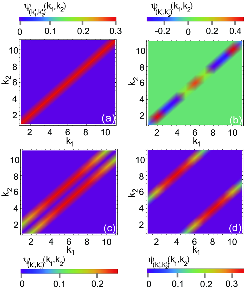
Figure 9: The amplitudes of $V$-basis states as defined by (100). (a) $k_{1}^{\prime}=k_{2}^{\prime}=0$ ($\Delta=0$ sector); (b) $k_{1}^{\prime}=0,k_{2}^{\prime}=3$ ($\Delta=0$ sector); (c) $k_{1}^{\prime}=N+1,k_{2}^{\prime}=0$ ($\Delta=1$ sector); (d) $k_{1}^{\prime}=7N-5,k_{2}^{\prime}=0$ ($\Delta=3$ sector). We use $N=10$ for our calculations.

VI Properties of the $V$-basis states

We have seen in Sec. IV and Sec. V that the effect of a long sequence of projections $T_{\vec{\Delta}}$ is to collapse an initial state onto one of the $V$-basis states. We examined a particular case in Sec. IV.2 where the state converges towards a maximally entangled state. In this section, we examine the nature of the remaining $V$-basis states. We again limit our analysis to an odd number of projections.

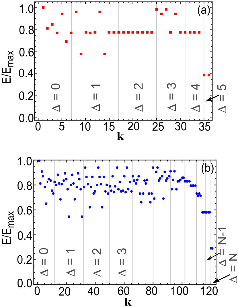
Figure 10: Entanglement of the $V$-basis states as defined by (50) for (a) $N=5$, (b) $N=10$. States are enumerated by $[\bm{k}]=k_{2}(N+1)+k_{1}$. Different states in each $\Delta$ sector are separated by vertical line. We have normalized with respect to the maximum entanglement between two BECs, $E_{\text{max}}=\log_{2}(N+1)$.

Figure 9 shows a gallery of states in the $V$-basis. We plot the coefficients

$$\psi_{k_{1}^{\prime}k_{2}^{\prime}}(k_{1},k_{2})=\langle k_{1},k_{2}|k_{1}^{\prime},k_{2}^{\prime}\rangle^{(V)}$$ (100)

for various choices of $k_{1}^{\prime},k_{2}^{\prime}$. We find that all states are diagonally correlated in $k_{1},k_{2}$. This is guaranteed from the fact that last projector $P_{\Delta^{z}_{L+1}}^{(z)}$ in the sequence is in the $z$-basis, and consists of correlated states according to (25). The $V$-basis states can be categorized into different sectors according to the $\Delta=\Delta^{z}_{L+1}$ of the final projection. The number of states in each sector is

$$n(\Delta)=\frac{2(N+1-\Delta)}{2^{\delta_{\Delta}}}$$ (101)

which is the same as the rank of each projector in (25). The states in each sector have different amplitude relations to ensure orthogonality (Fig. 9(a)(b)).

The diagonal nature of the states ensure that all the $V$-basis states are entangled. The degree of entanglement however depends upon which of the states $k_{1}^{\prime},k_{2}^{\prime}$ is obtained. Fig. 10 shows the entanglement of the states quantified by the von Neumann entropy (50) that is normalized with respect to the maximum entanglement between two BECs.

The reduced density matrix on BEC 1 is

$$\rho=\text{Tr}_{2}|k_{1}^{\prime},k_{2}^{\prime}\rangle^{(V)}\langle k_{1}^{\prime},k_{2}^{\prime}|^{(V)}.$$ (102)

From Fig. 10, we see that all states are entangled to various degrees. The maximally entangled state $E=E_{\text{max}}$ corresponds to the EPR state (47). The lowest entanglement is achieved in the $\Delta=N$ sector, corresponding to $E=1$. This corresponds to the states

$$\frac{1}{\sqrt{2}}(|N,0\rangle\pm|0,N\rangle)$$ (103)

which are NOON states. Since all the $V$-basis states are entangled, the sequential projection will drive an arbitrary state into an entangled state.

VII Summary and Conclusions

We have developed a theory of entangling QND measurements between atomic ensembles based on measurement operators. We first formulated the theory as developed in Ref. Aristizabal-Zuluaga et al. (2021) in terms of POVMs. We then examined a limiting case of the theory with $|\alpha\tau|^{2}>1$ where two POVMs reduce to projection operators. This clarifies the way in which entanglement is generated in the system, but also reveals why non-maximal entanglement is generated with a single QND projection (see for e.g. (34)). We then proceeded to analyze the multiple projection case, where a sequence of projections in alternating $z$ and $x$ bases are made. Using a key mathematical observation (Lemma 1), the multiple projections can be simplified greatly. This resulted in Theorem 1, where it was found that it is possible to evaluate an arbitrary sequence of projections very efficiently, using only a set of recursion relations of the state labels and associated amplitudes. The same situation can be analyzed in a statistical sense using density matrices, where the convergent state can be obtained for a large number of projections.

The main difference between our results and past works is to firstly formulate the QND entangling operation as an exact POVM or projection operator. Past methods rely on using various approximation to the spins (e.g. a Holstein-Primakoff approximation). Since our theory is based upon Ref. Aristizabal-Zuluaga et al. (2021) which treats the spin dynamics exactly, the POVM formulation is an exact solution of the QND dynamics. The projection operator is a particular limiting case of this theory, but should be very accurate for the large photon regime that experiments are typically carried out in. Secondly, we have shown that a sequence of multiple QND measurements (i.e. the stroboscopic measurements) has a very simple mathematical structure that can be exploited. This yields a method to obtain the state after a number of measurements in a very efficient way. Normally, the projection sequence requires a calculation that scales as $(2L+1)(N+1)^{6}$, and there is little intuition to the procedure. We have shown that there is a particular basis in which the states collapse to (the $U$ and $V$-basis), and makes clear the nature of the state that is obtained in the procedure.

The projected sequence to prepare a maximally entangled state as shown in Sec. IV.2 is very attractive as a fundamental state preparation protocol for use in quantum information applications. It allows for a way of enhancing the spin correlations and can generate a highly entangled state of atomic ensembles. A prime application is spinor quantum computing Byrnes et al. (2012, 2015), where one deals with a many-body wavefunction to encode the logical states, and a regime away from the conventional Holstein-Primakoff approximated states are used. Hence it is important to know the effect of such entangling operations such that they can be used for quantum information applications. However, it should be pointed out that this is not deterministic, and represents merely one particular measurement outcome. This is similar to the one-ensemble counterpart as experimentally demonstrated in Ref. Behbood et al. (2014) where post-selection was used to target the entangled singlet state. Due to the large Hilbert space of atomic ensembles, a more desirable scheme would be deterministic preparation of a target entangled state. For the one-ensemble case, feedback approaches were examined to achieve this Behbood et al. (2013b). We leave investigation of such deterministic schemes as future work.

Appendix A Proof of Lemma 1

In this section we show that the commutative property (56) holds. First note that for $\Delta^{z}\neq{\Delta^{z}}^{\prime}$

$$R_{\Delta^{z}\Delta^{x}}R_{{\Delta^{z}}^{\prime}{\Delta^{x}}^{\prime}}=P_{\Delta^{z}}^{(z)}P_{{\Delta^{x}}}^{(x)}P_{\Delta^{z}}^{(z)}P_{{\Delta^{z}}^{\prime}}^{(z)}P_{{\Delta^{x}}^{\prime}}^{(x)}P_{{\Delta^{z}}^{\prime}}^{(z)}=0$$ (104)

from the orthogonality of projection matrices. Thus for $\Delta^{z}\neq{\Delta^{z}}^{\prime}$ the commutative relation (56) holds trivially. Thus we only need to prove (56) for the $\Delta^{z}={\Delta^{z}}^{\prime}$ case, and our task will be to prove the equivalent relation

$$P_{\Delta^{z}}^{(z)}P_{{\Delta^{x}}^{\prime}}^{(x)}P_{\Delta^{z}}^{(z)}P_{{\Delta^{x}}^{\prime\prime}}^{(x)}P_{\Delta^{z}}^{(z)}{=}P_{\Delta^{z}}^{(z)}P_{{\Delta^{x}}^{\prime\prime}}^{(x)}P_{\Delta^{z}}^{(z)}P_{{\Delta^{x}}^{\prime}}^{(x)}P_{\Delta^{x}}^{(x)}.$$ (105)

Next let us write the relation (105) in an alternative form by defining new projection operators

$$\Pi_{\delta}^{(l)}=\sum_{k}|k,k+\delta\rangle\langle k,k+\delta|^{(l)}$$ (106)

where $\delta$ can be a positive or negative integer, and $l\in\{x,z\}$ indicates the basis. Then our original projection operators (25) are

$$P_{\Delta}^{(l)}=\Pi_{\Delta}^{(l)}+\Pi_{-\Delta}^{(l)}=\sum_{\sigma=\pm 1}\Pi_{\sigma\Delta}^{(l)}.$$ (107)

The relation that we wish to prove (105) can be rewritten in terms of the new projection operators as

$$\sum_{\sigma_{1}\sigma_{2}\sigma_{3}\sigma_{4}\sigma_{5}}\Big{(}\Pi_{{\sigma_{1}\Delta^{z}}}^{(z)}\Pi_{{\sigma_{2}\Delta^{x}}^{\prime}}^{(x)}\Pi_{\sigma_{3}\Delta^{z}}^{(z)}\Pi_{{\sigma_{4}\Delta^{x}}^{\prime\prime}}^{(x)}\Pi_{{\sigma_{5}\Delta^{z}}}^{(z)}$$

$$-\Pi_{{\sigma_{1}\Delta^{z}}}^{(z)}\Pi_{{\sigma_{4}\Delta^{x}}^{\prime\prime}}^{(x)}\Pi_{\sigma_{3}\Delta^{z}}^{(z)}\Pi_{{\sigma_{2}\Delta^{x}}^{\prime}}^{(x)}\Pi_{{\sigma_{5}\Delta^{z}}}^{(z)}\Big{)}=0.$$ (108)

it is possible to relabel the $\sigma_{i}$ variables since they are dummy indices, and we have made a convenient choice for the purposes of our proof. We will show that the quantity inside parentheses is always zero, proving the desired relation.

The key insight to proving the desired relation is to notice that the projectors (106) project the two BECs onto an eigenstate of $S^{z}_{1}-S^{z}_{2}$, such that the spin difference between the BECs is fixed. It will be convenient to transform the projectors such that instead of a spin difference, the projectors (106) project on to the total spin $S^{z}_{1}+S^{z}_{2}$. This can be achieved by flipping the second spin such that the transformed state is

$$e^{iS^{y}_{2}\frac{\pi}{2}}|k\rangle=(-1)^{k}|N-k\rangle.$$ (109)

We can therefore define the rotated projection operator

$$\tilde{\Pi}_{\Delta}^{(z)} =e^{iS^{y}_{2}\frac{\pi}{2}}\Pi_{\Delta}^{(z)}e^{-iS^{y}_{2}\frac{\pi}{2}}$$

$$=\sum_{k}|k,N-k-\Delta\rangle\langle k,N-k-\Delta|,$$ (110)

which consists of states with total spin $S^{z}_{1}+S^{z}_{2}=-2\Delta$.

Let us now change the notation of the Fock states such that they are instead interpreted as angular momentum eigenstates. For a single BEC, we may write Byrnes and Ilo-Okeke (2021)

$$|k\rangle=\Big{|}j=\frac{N}{2},m=k-\frac{N}{2}\Big{\rangle}$$ (111)

where ‘$j$’ is the angular momentum quantum number and ‘$m$’ is the quantum number associated with the spin along the $z$-direction. Then the rotated projectors can be written in this notation

$$\tilde{\Pi}_{\Delta}^{(z)}=\sum_{m} |j_{1}=\frac{N}{2},m;j_{2}=\frac{N}{2},-m-\Delta\rangle$$

$$\langle j_{1}=\frac{N}{2},m;j_{2}=\frac{N}{2},-m-\Delta|.$$ (112)

Now we may rewrite the states in (112) in terms of the total angular momentum basis $|J,M\rangle$, consisting of two individual spins of equal angular momenta $j_{1}=j_{2}=\frac{N}{2}$. The total spin operator is defined

$$\bm{J}=\bm{j}_{1}+\bm{j}_{2}=\frac{\bm{S}_{1}+\bm{S}_{2}}{2}.$$ (113)

The conversion between the bases is achieved by Clebsch-Gordan coefficients

$$|j_{1},m_{1};j_{2},m_{2}\rangle= \sum_{J=|j_{1}-j_{2}|}^{j_{1}+j_{2}}|J,M=m_{1}+m_{2}\rangle$$

$$\times\langle J,M=m_{1}+m_{2}|j_{1},m_{1};j_{2},m_{2}\rangle.$$ (114)

Substituting this into (112), we obtain

$$\tilde{\Pi}_{\Delta}^{(z)}=\sum_{J}|J,-\Delta\rangle^{(z)}\langle J,-\Delta|^{(z)}.$$ (115)

Here we used the $m$-sum unitarity relation for Clebsch-Gordan coefficients Thompson (2008),

$$\sum_{m_{1},m_{2}} \langle J^{\prime},M^{\prime}|j_{1},m_{1};j_{2},m_{2}\rangle\langle j_{1},m_{1};j_{2},m_{2}|J,M\rangle$$

$$=\delta_{JJ^{\prime}}\delta_{MM^{\prime}}.$$ (116)

The sum in (115) is over all total angular momentum states that have the same $J^{z}$ eigenvalue. Similarly, we have the projectors defined in the $x$-basis

$$\tilde{\Pi}_{\Delta^{x}}^{(x)} =e^{-iJ^{y}\frac{\pi}{4}}\tilde{\Pi}_{\Delta}^{(z)}e^{iJ^{y}\frac{\pi}{4}}$$ (117)

$$=\sum_{J}|J,-\Delta\rangle^{(x)}\langle J,-\Delta|^{(x)}$$

Let us now evaluate the sequence of projectors

$$\tilde{\Pi}_{\Delta}^{(z)}\tilde{\Pi}_{{\Delta_{2}}}^{(x)}\tilde{\Pi}_{\Delta_{3}}^{(z)}\tilde{\Pi}_{{\Delta_{4}}}^{(x)}\tilde{\Pi}_{\Delta}^{(z)}=\sum_{J}|J,-\Delta\rangle^{(z)}\langle J,-\Delta|^{(z)}$$

$$\times d_{-\Delta,-\Delta_{2}}^{J}d_{-\Delta_{3},-\Delta_{2}}^{J}d_{-\Delta_{3},-\Delta_{4}}^{J}d_{-\Delta,-\Delta_{4}}^{J},$$ (118)

where we used the fact that a rotation of the angular momentum states preserves $J$ Thompson (2008)

$$\text{}^{(z)}\langle J,M|J^{\prime},M^{\prime}\rangle^{(x)} =\text{}^{(z)}\langle J,M|e^{-iJ^{y}\frac{\pi}{4}}|J^{\prime},M^{\prime}\rangle^{(z)}$$

$$=\delta_{J,J^{\prime}}d^{J}_{M,M^{\prime}},$$ (119)

and we defined

$$d^{J}_{M,M^{\prime}}=\text{}^{(z)}\langle J,M|J,M^{\prime}\rangle^{(x)}.$$ (120)

We may also evaluate the sequence with the ordering of the $\Delta_{2}$ and $\Delta_{4}$ interchanged

$$\tilde{\Pi}_{\Delta}^{(z)}\tilde{\Pi}_{{\Delta_{4}}}^{(x)}\tilde{\Pi}_{\Delta_{3}}^{(z)}\tilde{\Pi}_{{\Delta_{2}}}^{(x)}\tilde{\Pi}_{\Delta}^{(z)}=\sum_{J}|J,-\Delta\rangle^{(z)}\langle J,-\Delta|^{(z)}$$

$$\times d_{-\Delta,-\Delta_{4}}^{J}d_{-\Delta_{3},-\Delta_{4}}^{J}d_{-\Delta_{3},-\Delta_{2}}^{J}d_{-\Delta,-\Delta_{2}}^{J}.$$ (121)

The right hand sides of (118) and (121) are the same, hence we establish that

$$\tilde{\Pi}_{\Delta}^{(z)}\tilde{\Pi}_{{\Delta_{2}}}^{(x)}\tilde{\Pi}_{\Delta_{3}}^{(z)}\tilde{\Pi}_{{\Delta_{4}}}^{(x)}\tilde{\Pi}_{\Delta}^{(z)}=\tilde{\Pi}_{\Delta}^{(z)}\tilde{\Pi}_{{\Delta_{4}}}^{(x)}\tilde{\Pi}_{\Delta_{3}}^{(z)}\tilde{\Pi}_{{\Delta_{2}}}^{(x)}\tilde{\Pi}_{\Delta}^{(z)}.$$ (122)

Now let us consider the sequence

$$\tilde{\Pi}_{\Delta}^{(z)}\tilde{\Pi}_{{\Delta_{2}}}^{(x)}\tilde{\Pi}_{\Delta_{3}}^{(z)}\tilde{\Pi}_{{\Delta_{4}}}^{(x)}\tilde{\Pi}_{-\Delta}^{(z)}=\sum_{J}|J,-\Delta\rangle^{(z)}\langle J,\Delta|^{(z)}$$

$$\times d_{-\Delta,-\Delta_{2}}^{J}d_{-\Delta_{3},-\Delta_{2}}^{J}d_{-\Delta_{3},-\Delta_{4}}^{J}d_{\Delta,-\Delta_{4}}^{J},$$ (123)

The sequence with $\Delta_{2}$ and $\Delta_{4}$ interchanged is

$$\tilde{\Pi}_{\Delta}^{(z)}\tilde{\Pi}_{{\Delta_{4}}}^{(x)}\tilde{\Pi}_{\Delta_{3}}^{(z)}\tilde{\Pi}_{{\Delta_{2}}}^{(x)}\tilde{\Pi}_{-\Delta}^{(z)}=\sum_{J}|J,-\Delta\rangle^{(z)}\langle J,\Delta\rangle^{(z)}$$

$$\times d_{-\Delta,-\Delta_{4}}^{J}d_{-\Delta_{3},-\Delta_{4}}^{J}d_{-\Delta_{3},-\Delta_{2}}^{J}d_{\Delta,-\Delta_{2}}^{J}.$$ (124)

Using the identity Thompson (2008)

$$\text{}^{(z)}\langle J,-M|J,M^{\prime}\rangle^{(x)} =\text{}^{(z)}\langle J,M|J,M^{\prime}\rangle^{(x)}(-1)^{J+M}$$ (125)

we have

$$d_{-M,M^{\prime}}^{J}=(-1)^{J+M}d_{M,M^{\prime}}^{J}.$$ (126)

Using this in relation we may equate the right hand sides of (123) and (124) and we establish that

$$\tilde{\Pi}_{\Delta}^{(z)}\tilde{\Pi}_{{\Delta_{2}}}^{(x)}\tilde{\Pi}_{\Delta_{3}}^{(z)}\tilde{\Pi}_{{\Delta_{4}}}^{(x)}\tilde{\Pi}_{-\Delta}^{(z)}=\tilde{\Pi}_{\Delta}^{(z)}\tilde{\Pi}_{{\Delta_{4}}}^{(x)}\tilde{\Pi}_{\Delta_{3}}^{(z)}\tilde{\Pi}_{{\Delta_{2}}}^{(x)}\tilde{\Pi}_{-\Delta}^{(z)}.$$ (127)

We may now write the results (122) and (127) in an equivalent form, by inverting the transformation (110) and removing the tildes from the projectors

$$\Pi_{\Delta}^{(z)}\Pi_{{\Delta}^{\prime\prime}}^{(x)}\Pi_{\Delta}^{(z)}\Pi_{{\Delta}^{\prime}}^{(x)}\Pi_{\Delta}^{(z)}=e^{-iS^{y}_{2}\frac{\pi}{2}}\tilde{\Pi}_{\Delta}^{(z)}\tilde{\Pi}_{{\Delta}^{\prime\prime}}^{(x)}\tilde{\Pi}_{\Delta}^{(z)}\tilde{\Pi}_{{\Delta}^{\prime}}^{(x)}\tilde{\Pi}_{\Delta}^{(z)}e^{iS^{y}_{2}\frac{\pi}{2}}.$$ (128)

Combining the two cases (122) and (127) into one relation we have

$$\Pi_{\Delta}^{(z)}\Pi_{{\Delta_{2}}}^{(x)}\Pi_{\Delta_{3}}^{(z)}\Pi_{{\Delta_{4}}}^{(x)}\Pi_{\pm\Delta}^{(z)}=\Pi_{\Delta}^{(z)}\Pi_{{\Delta_{4}}}^{(x)}\Pi_{\Delta_{3}}^{(z)}\Pi_{{\Delta_{2}}}^{(x)}\Pi_{\pm\Delta}^{(z)}.$$ (129)

We may now prove the desired relation (108). Setting $\Delta=\sigma_{1}\Delta^{z}$, $\Delta_{2}=\sigma_{2}{\Delta^{x}}^{\prime}$, $\Delta_{3}=\sigma_{3}\Delta^{z}$, $\Delta_{4}=\sigma_{4}{\Delta^{x}}^{\prime\prime}$ and applying (129), for cases with $\sigma_{1}=\sigma_{5}$ the content of the brackets in (108) is zero, according to the $+$ version of (129). For cases with $\sigma_{1}=-\sigma_{5}$, we can apply the $-$ version of (129), and the quantity inside the brackets in (108) is again zero. This proves the desired relation.

Appendix B An example of Lemma 1

We provide an explicit example for $N=2$. The rotation matrix (27) can be evaluated using Eq. (5.162) and (5.163) in Ref. Byrnes and Ilo-Okeke (2021). The rotation matrix is for this case

$${\cal U}(\frac{\pi}{2},0)=\frac{1}{4}\left(\begin{array}[]{ccc}U_{1}&U_{2}&U_{1}\\ -U_{2}&U_{3}&U_{2}\\ U_{1}&-U_{2}&U_{1}\\ \end{array}\right)$$ (133)

where we defined

$$U_{1} =\left(\begin{array}[]{ccc}1&-\sqrt{2}&1\\ \sqrt{2}&0&-\sqrt{2}\\ 1&\sqrt{2}&1\\ \end{array}\right)$$ (137)

$$U_{2} =\left(\begin{array}[]{ccc}-\sqrt{2}&2&-\sqrt{2}\\ -2&0&2\\ -\sqrt{2}&-2&-\sqrt{2}\\ \end{array}\right)$$ (141)

$$U_{3} =\left(\begin{array}[]{ccc}0&0&0\\ 0&0&0\\ 0&0&0\\ \end{array}\right).$$ (145)

This can be used to calculated the sequence of two projectors as in (52). For example, for $\Delta^{z}=\Delta^{x}=0$

$$T_{00}=\frac{1}{8}\left(\begin{array}[]{ccccccccc}3&0&0&0&2&0&0&0&3\\ 0&0&0&0&0&0&0&0&0\\ -1&0&0&0&2&0&0&0&-1\\ 0&0&0&0&0&0&0&0&0\\ 2&0&0&0&4&0&0&0&2\\ 0&0&0&0&0&0&0&0&0\\ -1&0&0&0&2&0&0&0&-1\\ 0&0&0&0&0&0&0&0&0\\ 3&0&0&0&2&0&0&0&3\\ \end{array}\right)$$ (155)

and for $\Delta^{z}=\Delta^{x}=2$

$$T_{22}=\frac{1}{8}\left(\begin{array}[]{ccccccccc}0&0&1&0&0&0&1&0&0\\ 0&0&0&0&0&0&0&0&0\\ 0&0&1&0&0&0&1&0&0\\ 0&0&0&0&0&0&0&0&0\\ 0&0&-2&0&0&0&-2&0&0\\ 0&0&0&0&0&0&0&0&0\\ 0&0&1&0&0&0&1&0&0\\ 0&0&0&0&0&0&0&0&0\\ 0&0&1&0&0&0&1&0&0\\ \end{array}\right).$$ (165)

The common unitary operators in (53) are

$$U=\left(\begin{array}[]{ccccccccc}\frac{1}{\sqrt{3}}&\frac{1}{2\sqrt{6}}&-\frac{1}{\sqrt{2}}&\frac{1}{2\sqrt{2}}&0&0&0&0&0\\ 0&0&0&0&\frac{1}{2}&-\frac{1}{\sqrt{2}}&0&\frac{1}{2}&0\\ 0&-\frac{\sqrt{\frac{3}{2}}}{2}&0&\frac{1}{2\sqrt{2}}&0&0&0&0&-\frac{1}{\sqrt{2}}\\ 0&0&0&0&\frac{1}{2}&0&-\frac{1}{\sqrt{2}}&-\frac{1}{2}&0\\ \frac{1}{\sqrt{3}}&-\frac{1}{\sqrt{6}}&0&-\frac{1}{\sqrt{2}}&0&0&0&0&0\\ 0&0&0&0&\frac{1}{2}&0&\frac{1}{\sqrt{2}}&-\frac{1}{2}&0\\ 0&-\frac{\sqrt{\frac{3}{2}}}{2}&0&\frac{1}{2\sqrt{2}}&0&0&0&0&\frac{1}{\sqrt{2}}\\ 0&0&0&0&\frac{1}{2}&\frac{1}{\sqrt{2}}&0&\frac{1}{2}&0\\ \frac{1}{\sqrt{3}}&\frac{1}{2\sqrt{6}}&\frac{1}{\sqrt{2}}&\frac{1}{2\sqrt{2}}&0&0&0&0&0\\ \end{array}\right)$$ (175)

and

$$V=\left(\begin{array}[]{ccccccccc}\frac{1}{\sqrt{3}}&\frac{1}{\sqrt{6}}&-\frac{1}{\sqrt{2}}&0&0&0&0&0&0\\ 0&0&0&\frac{1}{2}&-\frac{1}{\sqrt{2}}&0&\frac{1}{2}&0&0\\ 0&0&0&0&0&0&0&\frac{1}{\sqrt{2}}&-\frac{1}{\sqrt{2}}\\ 0&0&0&\frac{1}{2}&0&-\frac{1}{\sqrt{2}}&-\frac{1}{2}&0&0\\ \frac{1}{\sqrt{3}}&-\sqrt{\frac{2}{3}}&0&0&0&0&0&0&0\\ 0&0&0&\frac{1}{2}&0&\frac{1}{\sqrt{2}}&-\frac{1}{2}&0&0\\ 0&0&0&0&0&0&0&\frac{1}{\sqrt{2}}&\frac{1}{\sqrt{2}}\\ 0&0&0&\frac{1}{2}&\frac{1}{\sqrt{2}}&0&\frac{1}{2}&0&0\\ \frac{1}{\sqrt{3}}&\frac{1}{\sqrt{6}}&\frac{1}{\sqrt{2}}&0&0&0&0&0&0\\ \end{array}\right).$$ (185)

The associated singular matrices are

$$\Lambda_{00}=\left(\begin{array}[]{ccccccccc}1&0&0&0&0&0&0&0&0\\ 0&\frac{1}{2}&0&0&0&0&0&0&0\\ 0&0&0&0&0&0&0&0&0\\ 0&0&0&0&0&0&0&0&0\\ 0&0&0&0&0&0&0&0&0\\ 0&0&0&0&0&0&0&0&0\\ 0&0&0&0&0&0&0&0&0\\ 0&0&0&0&0&0&0&0&0\\ 0&0&0&0&0&0&0&0&0\\ \end{array}\right)$$ (195)

and

$$\Lambda_{22}=\left(\begin{array}[]{ccccccccc}0&0&0&0&0&0&0&0&0\\ 0&0&0&0&0&0&0&0&0\\ 0&0&0&0&0&0&0&0&0\\ 0&0&0&0&0&0&0&\frac{1}{2}&0\\ 0&0&0&0&0&0&0&0&0\\ 0&0&0&0&0&0&0&0&0\\ 0&0&0&0&0&0&0&0&0\\ 0&0&0&0&0&0&0&0&0\\ 0&0&0&0&0&0&0&0&0\\ \end{array}\right).$$ (205)

References

• Einstein et al. (1935) A. Einstein, B. Podolsky, and N. Rosen, Phys. Rev. 47, 777 (1935).
• Horodecki et al. (2009) R. Horodecki, P. Horodecki, M. Horodecki, and K. Horodecki, Rev. Mod. Phys. 81, 865 (2009).
• Chitambar and Gour (2019) E. Chitambar and G. Gour, Rev. Mod. Phys. 91, 025001 (2019).
• Wilde (2013) M. M. Wilde, Quantum information theory (Cambridge University Press, 2013).
• Bouwmeester and Zeilinger (2000) D. Bouwmeester and A. Zeilinger, in The physics of quantum information (Springer, 2000), pp. 1–14.
• Schleich et al. (2016) W. P. Schleich, K. S. Ranade, C. Anton, M. Arndt, M. Aspelmeyer, M. Bayer, G. Berg, T. Calarco, H. Fuchs, E. Giacobino, et al., Applied Physics B 122, 130 (2016).
• Ladd et al. (2010) T. D. Ladd, F. Jelezko, R. Laflamme, Y. Nakamura, C. Monroe, and J. L. O’Brien, Nature 464, 45 (2010).
• Mermin (2007) N. D. Mermin, Quantum computer science: an introduction (Cambridge University Press, 2007).
• Preskill (2012) J. Preskill, arXiv preprint arXiv:1203.5813 (2012).
• Amico et al. (2008) L. Amico, R. Fazio, A. Osterloh, and V. Vedral, Rev. Mod. Phys. 80, 517 (2008).
• Its et al. (2005) A. R. Its, B.-Q. Jin, and V. E. Korepin, Journal of Physics A: Mathematical and General 38, 2975 (2005).
• Zhang and Li (2005) G.-F. Zhang and S.-S. Li, Physical Review A 72, 034302 (2005).
• Latorre and Riera (2009) J. Latorre and A. Riera, Journal of physics a: mathematical and theoretical 42, 504002 (2009).
• Arunkumar et al. (2019) N. Arunkumar, A. Jagannathan, and J. E. Thomas, Phys. Rev. Lett. 122, 040405 (2019).
• Hammerer et al. (2010) K. Hammerer, A. S. Sørensen, and E. S. Polzik, Reviews of Modern Physics 82, 1041 (2010).
• Lukin et al. (2000) M. D. Lukin, S. F. Yelin, and M. Fleischhauer, Phys. Rev. Lett. 84, 4232 (2000).
• Sørensen et al. (2001) A. Sørensen, L.-M. Duan, J. Cirac, and P. Zoller, Nature 409, 63 (2001).
• Hald et al. (1999) J. Hald, J. L. Sørensen, C. Schori, and E. S. Polzik, Phys. Rev. Lett. 83, 1319 (1999).
• Kuzmich et al. (2000) A. Kuzmich, L. Mandel, and N. P. Bigelow, Phys. Rev. Lett. 85, 1594 (2000).
• Esteve et al. (2008) J. Esteve, C. Gross, A. Weller, S. Giovanazzi, and M. Oberthaler, Nature 455, 1216 (2008).
• Kunkel et al. (2018) P. Kunkel, M. Prüfer, H. Strobel, D. Linnemann, A. Frölian, T. Gasenzer, M. Gärttner, and M. K. Oberthaler, Science 360, 413 (2018).
• Fadel et al. (2018) M. Fadel, T. Zibold, B. Décamps, and P. Treutlein, Science 360, 409 (2018).
• Gross (2012) C. Gross, Journal of Physics B: Atomic, Molecular and Optical Physics 45, 103001 (2012).
• Giovannetti et al. (2006) V. Giovannetti, S. Lloyd, and L. Maccone, Phys. Rev. Lett. 96, 010401 (2006).
• Giovannetti et al. (2004) V. Giovannetti, S. Lloyd, and L. Maccone, Science 306, 1330 (2004).
• Tóth and Apellaniz (2014) G. Tóth and I. Apellaniz, Journal of Physics A: Mathematical and Theoretical 47, 424006 (2014).
• Giovannetti et al. (2011) V. Giovannetti, S. Lloyd, and L. Maccone, Nature photonics 5, 222 (2011).
• Bao et al. (2020) H. Bao, J. Duan, S. Jin, X. Lu, P. Li, W. Qu, M. Wang, I. Novikova, E. E. Mikhailov, K.-F. Zhao, et al., Nature 581, 159 (2020).
• Sekatski et al. (2017) P. Sekatski, M. Skotiniotis, J. Kołodyński, and W. Dür, Quantum 1, 27 (2017), ISSN 2521-327X.
• Bell (1964) J. S. Bell, Physics Physique Fizika 1, 195 (1964), URL https://link.aps.org/doi/10.1103/PhysicsPhysiqueFizika.1.195.
• Freedman and Clauser (1972) S. J. Freedman and J. F. Clauser, Physical Review Letters 28, 938 (1972).
• Aspect et al. (1982) A. Aspect, J. Dalibard, and G. Roger, Physical review letters 49, 1804 (1982).
• Adesso et al. (2016) G. Adesso, T. R. Bromley, and M. Cianciaruso, Journal of Physics A: Mathematical and Theoretical 49, 473001 (2016).
• Ma et al. (2019) Z.-H. Ma, J. Cui, Z. Cao, S.-M. Fei, V. Vedral, T. Byrnes, and C. Radhakrishnan, EPL (Europhysics Letters) 125, 50005 (2019).
• Schmied et al. (2016) R. Schmied, J.-D. Bancal, B. Allard, M. Fadel, V. Scarani, P. Treutlein, and N. Sangouard, Science 352, 441 (2016).
• Lloyd (1996) S. Lloyd, Science 273, 1073 (1996).
• Buluta and Nori (2009) I. Buluta and F. Nori, Science 326, 108 (2009).
• Byrnes and Ilo-Okeke (2021) T. Byrnes and E. O. Ilo-Okeke, Quantum Atom Optics: Theory and Applications to Quantum Technology (Cambridge University Press, 2021).
• Jané et al. (2003) E. Jané, G. Vidal, W. Dür, P. Zoller, and J. I. Cirac, Quantum Info. Comput. 3, 15–37 (2003), ISSN 1533-7146.
• You et al. (2017) C. You, S. Adhikari, Y. Chi, M. L. LaBorde, C. T. Matyas, C. Zhang, Z. Su, T. Byrnes, C. Lu, J. P. Dowling, et al., Journal of Optics 19, 124002 (2017).
• Horikiri et al. (2016) T. Horikiri, M. Yamaguchi, K. Kamide, Y. Matsuo, T. Byrnes, N. Ishida, A. Löffler, S. Höfling, Y. Shikano, T. Ogawa, et al., Scientific reports 6, 1 (2016).
• Lewenstein et al. (2007) M. Lewenstein, A. Sanpera, V. Ahufinger, B. Damski, A. Sen, and U. Sen, Advances in Physics 56, 243 (2007).
• Monroe et al. (2021) C. Monroe, W. C. Campbell, L.-M. Duan, Z.-X. Gong, A. V. Gorshkov, P. W. Hess, R. Islam, K. Kim, N. M. Linke, G. Pagano, et al., Reviews of Modern Physics 93, 025001 (2021).
• Julsgaard et al. (2001) B. Julsgaard, A. Kozhekin, and E. S. Polzik, Nature 413, 400 (2001).
• Krauter et al. (2013) H. Krauter, D. Salart, C. Muschik, J. M. Petersen, H. Shen, T. Fernholz, and E. S. Polzik, Nature Physics 9, 400 (2013).
• Braunstein and van Loock (2005) S. L. Braunstein and P. van Loock, Rev. Mod. Phys. 77, 513 (2005).
• Lange et al. (2018) K. Lange, J. Peise, B. Lücke, I. Kruse, G. Vitagliano, I. Apellaniz, M. Kleinmann, G. Tóth, and C. Klempt, Science 360, 416 (2018).
• Li et al. (2013) L. Li, Y. Dudin, and A. Kuzmich, Nature 498, 466 (2013).
• Pyrkov and Byrnes (2013) A. N. Pyrkov and T. Byrnes, New Journal of Physics 15, 093019 (2013).
• Rosseau et al. (2014) D. Rosseau, Q. Ha, and T. Byrnes, Physical Review A 90, 052315 (2014).
• Ortiz et al. (2018) S. Ortiz, Y. Song, J. Wu, V. Ivannikov, and T. Byrnes, Physical Review A 98, 043616 (2018).
• Hussain et al. (2014) M. I. Hussain, E. O. Ilo-Okeke, and T. Byrnes, Physical Review A 89, 053607 (2014).
• Abdelrahman et al. (2014) A. Abdelrahman, T. Mukai, H. Häffner, and T. Byrnes, Optics express 22, 3501 (2014).
• Idlas et al. (2016) S. Idlas, L. Domenzain, R. Spreeuw, and T. Byrnes, Physical Review A 93, 022319 (2016).
• Treutlein et al. (2006) P. Treutlein, T. W. Hänsch, J. Reichel, A. Negretti, M. A. Cirone, and T. Calarco, Phys. Rev. A 74, 022312 (2006).
• Oudot et al. (2017) E. Oudot, J.-D. Bancal, R. Schmied, P. Treutlein, and N. Sangouard, Phys. Rev. A 95, 052347 (2017).
• Jing et al. (2019) Y. Jing, M. Fadel, V. Ivannikov, and T. Byrnes, New Journal of Physics 21, 093038 (2019).
• Pyrkov and Byrnes (2014a) A. N. Pyrkov and T. Byrnes, New Journal of Physics 16, 073038 (2014a).
• Pyrkov and Byrnes (2014b) A. N. Pyrkov and T. Byrnes, Physical Review A 90, 062336 (2014b).
• Ilo-Okeke et al. (2018) E. O. Ilo-Okeke, L. Tessler, J. P. Dowling, and T. Byrnes, npj Quantum Information 4, 1 (2018).
• Chaudhary et al. (2021) M. Chaudhary, M. Fadel, E. O. Ilo-Okeke, A. N. Pyrkov, V. Ivannikov, and T. Byrnes, Phys. Rev. A 103, 062417 (2021).
• Byrnes et al. (2012) T. Byrnes, K. Wen, and Y. Yamamoto, Phys. Rev. A 85, 040306(R) (2012).
• Byrnes et al. (2015) T. Byrnes, D. Rosseau, M. Khosla, A. Pyrkov, A. Thomasen, T. Mukai, S. Koyama, A. Abdelrahman, and E. Ilo-Okeke, Optics Communications 337, 102 (2015).
• Aristizabal-Zuluaga et al. (2021) J. E. Aristizabal-Zuluaga, I. Skobleva, L. Richter, Y. Ji, Y. Mao, M. Kondappan, V. Ivannikov, and T. Byrnes, Journal of Physics B: Atomic, Molecular and Optical Physics 54, 105502 (2021).
• Pettersson and Byrnes (2017) O. Pettersson and T. Byrnes, Physical Review A 95, 043817 (2017).
• Ilo-Okeke and Byrnes (2014) E. O. Ilo-Okeke and T. Byrnes, Physical review letters 112, 233602 (2014).
• Duan et al. (2000) L.-M. Duan, J. I. Cirac, P. Zoller, and E. S. Polzik, Phys. Rev. Lett. 85, 5643 (2000).
• Serafin et al. (2021) A. Serafin, M. Fadel, P. Treutlein, and A. Sinatra, Physical Review Letters 127, 013601 (2021).
• Tsang and Caves (2012) M. Tsang and C. M. Caves, Physical Review X 2, 031016 (2012).
• Behbood et al. (2013a) N. Behbood, F. Martin Ciurana, G. Colangelo, M. Napolitano, M. W. Mitchell, and R. J. Sewell, Applied physics letters 102, 173504 (2013a).
• Behbood et al. (2014) N. Behbood, F. Martin Ciurana, G. Colangelo, M. Napolitano, G. Tóth, R. J. Sewell, and M. W. Mitchell, Phys. Rev. Lett. 113, 093601 (2014).
• Behbood et al. (2013b) N. Behbood, G. Colangelo, F. Martin Ciurana, M. Napolitano, R. J. Sewell, and M. W. Mitchell, Phys. Rev. Lett. 111, 103601 (2013b).
• Kitzinger et al. (2020) J. Kitzinger, M. Chaudhary, M. Kondappan, V. Ivannikov, and T. Byrnes, Physical Review Research 2, 033504 (2020).
• Nielsen and Chuang (2011) M. Nielsen and I. Chuang, Quantum Computation and Quantum Information: 10th Anniversary Edition (Cambridge University Press, New York, NY, USA, 2011), 10th ed., ISBN 1107002176, 9781107002173.
• Vasilakis et al. (2015) G. Vasilakis, H. Shen, K. Jensen, M. Balabas, D. Salart, B. Chen, and E. S. Polzik, Nature Physics 11, 389 (2015).
• Thompson (2008) W. J. Thompson, Angular momentum: an illustrated guide to rotational symmetries for physical systems (John Wiley & Sons, 2008).