Capsule Graph Neural Networks with EM Routing

Abstract.

To effectively classify graph instances, graph neural networks need to have the capability to capture the part-whole relationship existing in a graph. A capsule is a group of neurons representing complicated properties of entities, which has shown its advantages in traditional convolutional neural networks. This paper proposed novel Capsule Graph Neural Networks that use the EM routing mechanism (CapsGNNEM) to generate high-quality graph embeddings. Experimental results on a number of real-world graph datasets demonstrate that the proposed CapsGNNEM outperforms nine state-of-the-art models in graph classification tasks.

1. Introduction

Recent years have witnessed the increasing attention to Graph Neural Networks (GNNs) (Scarselli et al., 2009; Bruna et al., 2014; Kipf and Welling, 2017; Veličković et al., 2018), which have demonstrated remarkable advantages in many tasks performing on graph-structured data, such as node classification (Kipf and Welling, 2017; Rong et al., 2020; Gao et al., 2019; Zhou et al., 2021), graph classification (Bacciu et al., 2018; Li et al., 2019), and link prediction (Zhang and Chen, 2018a; Ragunathan et al., 2020). GNNs are generalized from traditional deep-learning models like CNNs and RNNs (handling grid or linear-structured data such as images and sequences), which can take graph-structured instances as their input. Many real-world data like social networks exhibit complicated graph structures. GNNs can be directly applied to the original graph structures, learning more effective representation.

This paper focuses on graph convolutional neural networks (GCNs), which employ convolutional operations for more general graph-structured data. The construction of GCNs can be categorized into spectral approaches and spatial approaches (Liu and Zhou, 2020). The common principle of both spectral and spatial convolutions is to recursively update node embeddings by aggregating information from topological neighbors, which can capture the local structure of nodes. The learned embeddings of nodes can be used in various tasks such as node classification and link prediction. To classify a whole graph instance, we need further to learn a graph embedding (a higher-level embedding compared with the node embedding), which is achieved by pooling methods (Zhang et al., 2018; Gao and Ji, 2019; Bianchi et al., 2020; Yuan and Ji, 2020). However, most existing graph pooling methods have two weaknesses: 1) The pooling operation may map different graphs or nodes into the same embedding, resulting in the model being incapable to capture meaningful information. 2) The pooling methods only consider the topology of the graph but ignore the part-whole relationships. For example, a molecule has a hydroxyl on its left and right sides, respectively. If they are not linked with each other, they will be clustered into different groups. However, because they have the same chemical properties they should be in the same group.

To solve the above issues, a group of neurons in the networks, namely capsule, was introduced, which encodes the activate probability of an entity as well as reserves the detailed properties of the entity such as position, direction, connection, and so on. Capsule neural networks have shown their effectiveness in modeling part-whole relationship on images (Hinton et al., 2011; Sabour et al., 2017; Hinton et al., 2018). It solves the viewpoint-invariant problem by transformation matrices. Capsule networks employ a routing mechanism to generate high-level capsules by the voting of low-level capsules. Compared with pooling methods that only reserve activated features, a routing mechanism preserves all information from low-level capsules and routes it to the closest high-level capsules. The most popular routing mechanism is dynamic routing by agreement (Sabour et al., 2017), which uses the length of a capsule to represent its degree of salience. Capsule and dynamic routing have been introduced in GNNs. CapsGNN (Zhang and Chen, 2018b) stacks the node features extracted by GCNs to build capsules and uses dynamic routing and attention mechanisms to generate high-level graph capsules as well as class capsules (Zhang and Chen, 2018b). GCAPS-CNN (Verma and Zhang, 2018) uses capsules to capture the highly informative output in a small vector in place of a scaler output currently employed in GCNs. The capsule is consists of higher-order statistical moments, which is permutationally invariant and can be computed via fast matrix multiplication. Another routing mechanism representing a capsule as matrices is matrix capsule with EM routing (Hinton et al., 2018). Using matrices instead of vectors to represent capsules can reduce the size of conversion matrices between capsules. For example, converting a $3\times 3$ matrix to a $3\times 6$ matrix requires a $3\times 6$ conversion matrix, while in dynamic routing converting a 9-dimensional vector to an 18-dimensional matrix requires a $9\times 18$ conversion matrix. Besides, the probability of an entity in EM routing is represented by a parameter $a$ (instead of a vector in dynamic routing), which avoids using the squashing function to ensure that the length of the vector is in a feasible range.

To the best of our knowledge, the matrix capsules with EM routing have never been introduced into GNNs. In this paper, we propose novel Capsule Graph Neural Networks with EM routing (CapsGNNEM), which uses node features extracted from GCN to generate high-quality graph embeddings by EM routing. Experimental results on a number of real-world graph datasets demonstrate the advantages of the proposed CapsGNNEM in graph classification.

2. Preliminaries

We first formulate graph classification and then briefly introduce graph neural networks and capsule neural networks.

Graph Classification

A graph is represented by $G=(V,X,A)$, where $V=\{v_{1},v_{2},v_{3},\cdots,v_{N}\}$ is a set of $N$ nodes, $X\in\mathbb{R}^{N\times C}$ is the feature matrix for nodes with feature channels $C$, and $A\in\{0,1\}^{N\times N}$ is the adjacency matrix. If there is an edge from $v_{i}$ to $v_{j}$, then we have $A_{ij}=1$, otherwise, $A_{ij}=0$. Given a set of labeled graphs $D=\{(G_{0},y_{0}),(G_{1},y_{1}),(G_{2},y_{2}),\cdots\}$, we aim to learn a graph embedding $g(G)\in\mathbb{R}^{k}$ for each graph, which encodes its attributes and structural information. Then, the graph representation (embeddings) can be used for graph classification.

Graph Neural Networks

Graph neural networks usually follow a neighborhood aggregation fashion to learn a node representation by applying a neighbor aggregation function to the representations of its neighbor nodes after propagation. More specifically, a neighbor aggregation function for the $i$-th node has the form:

(1) $$h_{i}^{(l+1)}=f(h_{i}^{(l)},\{h_{v}^{(l)}|v\in\mathcal{N}(v)\}),$$

where $\mathcal{N}(v)$ is a set of neighbors of node $i$ and $h_{i}^{(l)}$ is the representation of node $i$ at layer $l$. In each layer, the representation of every node is updated by the neighbor aggregation function. In graph classification, we need the representation of a whole graph, which usually can be obtained by simply summing up or averaging all the node embeddings on the graph. It obviously cannot capture the structural information of graphs. In capsule neural networks, graph embeddings are calculated by a hierarchical stack of capsules. The lowest-level capsules are the matrix presentation of nodes.

Capsule Neural Networks

A capsule is a group of neurons whose outputs represent different properties of an entity such as pose, deformation, texture, etc (Hinton et al., 2011). Routing algorithms are critical to the formation of different levels of capsules. In dynamic routing by agreement, the activation $\in([0,1)$ of a capsule is represented by its revised length after being calculated by a squashing function. The squashing function ensures that a short vector shrinks to a length slightly greater than $0$ and a long vector shrinks to a length slightly less than $1$, defined as $v_{j}=\frac{\left\lVert s_{j}\right\rVert^{2}}{1+\left\lVert s_{j}\right\rVert^{2}}\frac{s_{j}}{\left\lVert s_{j}\right\rVert}$, where $s_{j}$ and $v_{j}$ are the capsules before and after squashing, respectively. Accordingly, EM routing defines a special value as the activation value of a capsule, representing the certainty of an entity (Hinton et al., 2018), which is of better interpretability than using the capsule length as its activation value. (The details of EM routing are in Section 3.3). Since the higher-level capsules are obtained through the voting mechanism by the lower-level capsules, the hierarchical capsules can model the relationship between the part and whole.

3. The Proposed Method

This section presents the proposed CapsGNNEM in details.

3.1. Network Architecture

Figure 1 shows the architecture of our GapsGNNEM. It consists of three key components: Primary Capsule Layer, Capsule Convolutional Layer, and Readout Layer. In the first component, it uses GCN to extract different receptive-field node features to form the primary capsules and uses adjacency to form the initial activations. In the second component, the EM routing is applied to obtain high-level graph capsules. Finally, in the third component, the capsule with the best activation representing the most significant embeddings is chosen to make predictions by a multilayer perceptron (MLP).

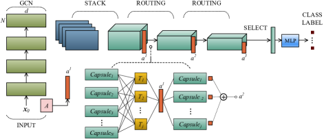
Figure 1. Architecture of the Proposed GapsGNNEM

3.2. Primary Capsule Layer

The goal of the primary capsule layer is to generate a capsule for each node on a graph. The features of a node are initialized with its original features. For those non-attribute graphs, we can choose Local Degree Profile (Chen and Wang, 2018) as the node attributes. The same as articles (Zhang and Chen, 2018b; Verma and Zhang, 2018), our method uses the GCN model (the commonest GNNs) (Kipf and Welling, 2017) to aggregate information from a node’s local neighborhood at a lower layer. The aggregation function at layer $l+1$ is as follows:

(2) $$X^{(l+1)}=f(\tilde{D}^{-1/2}\tilde{A}\tilde{D}^{-1/2}X^{(l)}\Theta),$$

where $f$ is a nonlinear activation function, $\tilde{A}=A+I_{N}$ and $\tilde{D}_{ij}=\sum_{j}\tilde{A}_{ij}$, $X^{(l)}\in\mathbb{R}^{N\times d}$ represents the $d$-dimensional features for all $N$ nodes at layer ${l}$ (particularly, $X^{(0)}=X$), and $\Theta\in\mathbb{R}^{d\times d^{\prime}}$ is a matrix of filter parameters that shrinks the dimension of node features from $d$ to $d^{\prime}$. As mentioned in the introduction, the matrix representation for a node is more efficient than vector representation. Thus, we stack the node features from different GCN layers to generate a matrix representation of features, which is consists of different receptive-field information. For example, if we have $k(\geq 3)$ GCN layers, the initial capsule for node $i$ is a $k\times d^{\prime}$ matrix $[X^{(1)}_{i:};X^{(2)}_{i:};\cdots;X^{(k)}_{i:}]$. The EM routing also requires an activation value. The bigger the degree of a node, the more central and important it is. Therefore, for node $i$, we intuitively choose its degree as the initial activation value, i.e., $a_{i}=\frac{D_{i}}{\sum_{j}D_{j}}$, where $D_{i}$ is its degree.

3.3. Capsule Convolutional Layer

After obtaining primary capsules and their initial activation values, the capsule convolutional layer decides how to assign lower-level active capsules to higher-level capsules. This process can be viewed as clustering (solved by an EM algorithm). Each higher-level capsule corresponds to a cluster center and each lower-level active capsule corresponds to a data point (or a fraction of a data point if the capsule is partially activated). First, it captures the part-whole relationship for each lower-level capsule $c_{i}^{(l)}$ and higher-level capsule $c_{j}^{(l+1)}$. This relationship is measured by a transformation matrix, which is called voting in EM routing and defined as follows:

(3) $$V_{ij}^{(l)}=c_{i}^{(l)}T_{ij}^{(l)},$$

where $V_{ij}^{(l)}\in\mathbb{R}^{k\times d^{\prime}}$ represents the voting result from capsule $i$ at layer $l$ for some capsule $j$ at layer $l+1$, $c_{i}^{(l)}$ represents capsule $i$ at layer $l$, and $T_{ij}^{(l)}$ is a transformation matrix. We use a simplified Gaussian Mixture Model (GMM) to generate higher-level capsules. That is, a higher-level capsule can be viewed as a center of multiple lower-level capsules. The simplified Gaussian distribution $\mathcal{N}(\bm{x};\bm{\mu},\Sigma)$ has a diagonal covariance matrix $diag(\bm{\sigma}^{2})$. In this settings, the posterior probability of a voting $V_{ij}$ belonging to the $j$-th Gaussian (i.e., capsule $j$ at the higher level) is

(4) $$R_{ij}=\frac{a_{j}\mathcal{N}(V_{ij};\bm{\mu}_{j},diag(\bm{\sigma}_{j}^{2}))}{\sum_{j}a_{j}\mathcal{N}(V_{ij};\bm{\mu}_{j},diag(\bm{\sigma}_{j}^{2}))},$$

where activation $a_{j}$ for capsule $j$ is a mixture coefficient of GMM and $V_{ij}$ is treated as a $k*d^{\prime}$-dimentional vector. Because lower-level capsules vote for a higher-level capsule $j$ the contribution coeffient $r_{ij}$ of capsule $i$ when calculating cluster center (capsule) $j$ should consider its activation value $a_{i}$ as follows:

(5) $$r_{ij}=\frac{a_{i}R_{ij}}{\sum_{i}a_{i}R_{ij}}.$$

Then, the parameters of the $j$-th Gaussian (parameter $\bm{\mu}_{j}$ is capsule $j$) can be updated in an EM procedure as follows:

(6) $$\bm{\mu}_{j}=\sum\limits_{i}r_{ij}V_{ij},$$

(7) $$(\sigma_{j}^{h})^{2}=\sum\limits_{i}r_{ij}(V_{ij}^{h}-\mu_{j}^{h})^{2},$$

where the superscript $h$ represents the $h$-th component of a vector. Following article (Hinton et al., 2018), the activation value for each capsule $j$ is calculated as follows:

$$cost_{j}^{h} =\sum\limits_{i}-r_{ij}\ln(p_{i|j}^{h})=\sum\limits_{i}r_{ij}(\ln(\sigma_{j}^{h})+1/2+\ln(2\pi)/2),$$

(8) $$a_{j} =logistic\left(\lambda\left(\beta_{a}-\beta_{u}\sum\limits_{i}r_{ij}-\sum\limits_{h}cost_{j}^{h}\right)\right),$$

where $p_{i|j}$ is the probability of $V_{ij}$ given capsule $j$ (i.e., $p_{i|j}=\mathcal{N}(V_{ij};\bm{\mu}_{j},diag(\bm{\sigma}_{j}^{2}))$), $cost_{j}$ represents the entropy of capsule $j$, $r_{ij}$ is the amount of votes assigned to capsule $j$, $\beta_{a}$ and $\beta_{u}$ are the learned parameters, and $\lambda$ is a hyper-parameter used to adjust the range of values to be better for the logistic function. Thus, $a_{j}$ represents the activation for capsule $j$ in the higher layer.

Finally, we summarize the whole EM routing in Algorithm 1.

Algorithm 1 EM routing algorithm returns activation values and capsules in layer $l+1$ given activation values and capsules in layer $l$. $\beta_{u}$ and $\beta_{a}$ are learned parameters and parameter $\lambda$ is fixed.

1:procedure EM routing($a^{in},X$)

2:     $R\leftarrow 1/|\Omega_{l+1}|,V\leftarrow\text{VOTING}(X)$ $\triangleright$ $\Omega_{l}$ stands for a set of capsules at layer $l$

3:     while $t\leq maxiter$ do

4:         $a^{out},\bm{\mu},\bm{\sigma}\leftarrow\text{M-STEP}(a^{in},R,V)$

5:         $R\leftarrow\text{E-STEP}(\bm{\mu},\bm{\sigma},a^{out},V)$      

6:     Return $a^{out},\bm{\mu}$

1:function VOTING($X$)

2:     $\forall i\in\Omega_{l},\forall j\in\Omega_{l+1}:$ calculate $V_{ij}$ by Eq. (3), where $c_{i}=X_{i}$

3:     Return $V$

1:function M-STEP($a^{in},R,V,j$)

2:     $\forall i\in\Omega_{l}:$ calculate $r_{ij}$ by Eq. (5)

3:     $\forall j\in\Omega_{l+1}:$ calculate $\bm{\mu}$, $\bm{\sigma}_{j}$, and $a_{j}^{out}$ by Eqs. (6), (7), and (8)

4:     Return $a^{out}$, $\bm{\mu}$, and $\bm{\sigma}_{j}$

1:function E-STEP($a^{out},V,\bm{\mu},\bm{\sigma}$)

2:     $\forall j\in\Omega_{l+1}:$ calculate $R_{ij}$ by Eq. (4), where $a_{j}=a^{out}$

3:     Return $R$

3.4. Readout Layer

The CNN-based capsule networks with EM routing (Hinton et al., 2018) directly use the activation value of the last layer to optimize with the spread loss function, which is very sensitive to hyper-parameter settings. Instead, we choose the capsule on the last layer with the best activation, which represents the most significant embedding. Then, we calculate the probability of each class using a fully connected layer and optimized it by the cross-entropy loss function. This will bring some robustness to our model when adjusting hyper-parameters.

Table 1. Comparison against nine state-of-the-art models on seven datasets in terms of accuracy (in percent)

$\mathbf{Algorithm}$	$\mathbf{MUTAG}$	$\mathbf{NCI1}$	$\mathbf{PROTEINS}$	$\mathbf{D\&D}$	$\mathbf{COLLAB}$	$\mathbf{IMDB-B}$	$\mathbf{IMDB-M}$
WL (Shervashidze et al., 2011)	$82.50\pm 0.36$	$82.19\pm 0.18$	$74.68\pm 0.49$	$79.78\pm 0.36$	$79.02\pm 1.77$	$73.40\pm 4.63$	$49.33\pm 4.75$
GK (Shervashidze et al., 2009)	$81.58\pm 2.11$	$62.49\pm 0.27$	$71.67\pm 0.55$	$78.45\pm 0.26$	$72.84\pm 0.28$	$65.87\pm 0.98$	$43.89\pm 0.38$
DGK (Yanardag and Vishwanathan, 2015)	$87.44\pm 2.72$	$80.31\pm 0.46$	$75.68\pm 0.54$	$73.50\pm 1.01$	$73.09\pm 0.25$	$66.96\pm 0.56$	$44.55\pm 0.52$
AWE (Ivanov and Burnaev, 2018)	$87.87\pm 9.76$	$78.18\pm 3.02$	$73.28\pm 2.64$	$71.51\pm 4.02$	$73.93\pm 1.94$	$74.45\pm 5.83$	$50.45\pm 3.61$
GCN (Kipf and Welling, 2017)	$87.20\pm 5.11$	$74.95\pm 0.64$	$75.65\pm 3.24$	$79.12\pm 3.07$	$\mathbf{81.72\pm 1.64}$	$73.30\pm 5.29$	$49.37\pm 2.21$
PSCN (Niepert et al., 2016)	$88.95\pm 4.37$	$76.34\pm 1.68$	$75.00\pm 2.51$	$76.27\pm 2.64$	$72.60\pm 2.15$	$71.00\pm 2.29$	$45.23\pm 2.84$
DGCNN (Zhang et al., 2018)	$85.83\pm 1.66$	$74.44\pm 0.47$	$75.54\pm 0.94$	$79.37\pm 0.94$	$73.76\pm 0.49$	$70.03\pm 0.86$	$47.83\pm 0.85$
GCAPS-CNN (Verma and Zhang, 2018)	$84.12\pm 3.19$	$\mathbf{82.72\pm 2.38}$	$76.40\pm 4.17$	$77.62\pm 4.99$	$77.71\pm 2.51$	$71.69\pm 3.40$	$48.50\pm 4.10$
CapsGNN (Zhang and Chen, 2018b)	$86.67\pm 6.88$	$78.35\pm 1.55$	$76.28\pm 3.63$	$75.38\pm 4.17$	$79.62\pm 0.91$	$73.10\pm 4.83$	$50.27\pm 2.65$
Ours (CapsGNNEM)	$\mathbf{90.51\pm 2.33}$	$75.03\pm 0.98$	$\mathbf{77.41\pm 1.12}$	$\mathbf{81.51\pm 4.31}$	$75.23\pm 1.47$	$\mathbf{75.40\pm 3.25}$	$\mathbf{50.87\pm 3.25}$

4. Experiments

In this section, we evaluate the performance of CapsGNNEM against a number of state-of-the-art graph classification methods.

4.1. Methods in Comparison

We compared the proposed CapsGNNEM with three categories of existing methods.

The first category is called kernel-based methods, including the Weisfeiler-Lehman subtree kernel (WL) (Shervashidze et al., 2011), the graphlet count kernel (GK) (Shervashidze et al., 2009), the deep graph kernel (DGK) (Yanardag and Vishwanathan, 2015), and anonymous walk embeddings (AWE) (Ivanov and Burnaev, 2018), which learn graph representation based on the substructs defined by the kernel methods.

The second category is called GNN-based methods. This category includes several methods. We selected five state-of-the-art GNN-based methods used in the experiments. GCN (Kipf and Welling, 2017) is one of the most influential models on graph neural networks. PATCHY-SAN (PSCN) (Niepert et al., 2016) selects a sequence of nodes and generates node representation by a receptive field, then uses CNN for graph classification. Deep Graph CNN (DGCNN) (Zhang et al., 2018) first uses a sorted pooling method to replace global pooling based on the node feature extracted by GNN, then uses CNN and MLP for classification.

The last category is called capsule-based methods. We included two capsule-based methods GCAPS-CNN (Verma and Zhang, 2018) and CapsGNN (Zhang and Chen, 2018b) in comparison. GCAPS-CNN uses higher-order statistical moments that are permutationally invariant to generate a capsule for each node, then computes covariance to deal with graph classification. CapsGNN generates capsules from multi-scale node embeddings extracted by GCN, then uses dynamic routing to generate graph embeddings for graph classification.

4.2. Experimental Settings

Seven real-world datasets were used in the experiments, which were derived from important application areas of graph classification, including four biological graph datasets (MUTAG, NCI1, PROTEINS, and D&D ) and three social network datasets (COLLAB, IMDB-B, and IMDB-M). The same hyper-parameter settings of CapsGNNEM were used for all datasets. For the primary capsule layer, we used 4 GCN layers to extract node features. The dimension of each node feature was set to 16. Thus, the dimension of a capsule after stacking is $4\times 16$. For the capsule convolutional layer, the number of output capsules is 3 times that of the following layer. The number of output capsules in the last layer is equal to the number of target classes. The number of iterations in the EM routing is set to 2 and the $\lambda$ is set to 0.1. We applied 10-fold cross-validation to evaluate the performance. For each evaluation process, the original instances were randomly partitioned into a training set and a test set. Then, we performed 10-fold cross-validation on the training set. In each cross-validation process, one fold of the training set was used to adjust and evaluate the performance of the trained model and the remainder was used to train a model. We selected the model with the best validation accuracy as a representative. The instances in the test set were predicted against the representative and the performance in terms of accuracy was evaluated. The above process was repeated 10 times, the average results and their standard deviations were reported.

4.3. Experimental Results

Table 1 lists the comparison results on the seven datasets in terms of accuracy. For each dataset, the average accuracy of the best model is in bold. Overall, our proposed CapGNNEM outperforms the other state-of-the-art methods on the datasets MUTAG, PROTEINS, D&D, IMDB-B, and IMDB-M. CapGNNEM wins on five out of seven datasets, which suggests that CapsGNNEM has the best overall performance. On three biological datasets (MUTAG, PROTEINS, and D&D), compared with two capsule-based methods (GCAPS-CNN and CapsGNN), CapsGNNEM improves the classification accuracy by margins of $3.84\%$, $1.01\%$ and $3.89\%$, respectively. The reason is that CapsGNNEM represents node features in form of capsules that can capture information of graphs from different aspects instead of only one embedding used in other GNN-based approaches. This is helpful to retain the properties of a graph when generating graph capsules. Besides, the capsule can capture the same properties and ignore the difference in their substruct, which is more important in biological datasets. These results also consistent with the property of EM routing, as it focuses more on extracting properties from child capsules by voting and routing. However, the social network datasets do not have node attributes. Therefore, applying routing to all child capsules leads to a loss of structural information in the graph. Therefore, even if CapsGNNEM has a higher average performance than other methods on IMDB-B and IMDB-M, comparing with the second-best methods, its margins of exceeding ($0.95$ on IMDB-B and $0.42$ on IMDB-M) are still smaller than those obtained from biological datasets. Nonetheless, CapsGNNEM still demonstrates its strong capability to capture graph properties and part-whole relationships.

5. Conclusion and Future Work

This paper proposes a novel CapsGNNEM model for graph classification, which combines capsule structures and graph convolutional networks. The capsules with EM routing not only can capture the properties and part-whole relations of graphs from GCN-extracted node features but also reduce the complexity of networks. Experimental results on a number of datasets have confirmed the advantages of the proposed model.

At present, the capsule convolution layer only performs global convolutions, which does not make good use of the structural information of the graph. In the future, we will construct a kind of local convolutions, where a cluster of capsules with a strong structural relationship is computed together. Moreover, since the model can represent hierarchical structures of capsules, the readout layer can extract hierarchical features as its input.

- (1)
- Bacciu et al. (2018) Davide Bacciu, Federico Errica, and Alessio Micheli. 2018. Contextual graph Markov model: A deep and generative approach to graph processing. In The 35th International Conference on Machine Learning (ICML). 294–303.
- Bianchi et al. (2020) Filippo Maria Bianchi, Daniele Grattarola, and Cesare Alippi. 2020. Spectral clustering with graph neural networks for graph pooling. In The 37th International Conference on Machine Learning (ICML). 874–883.
- Bruna et al. (2014) Joan Bruna, Wojciech Zaremba, Arthur Szlam, and Yann LeCun. 2014. Spectral networks and locally connected networks on graphs. In The 2nd International Conference on Learning Representations (ICLR).
- Chen and Wang (2018) Cai Chen and Yusu Wang. 2018. A simple yet effective baseline for non-attribute graph classification. ArXiv abs/1811.03508 (2018).
- Gao and Ji (2019) Hongyang Gao and Shuiwang Ji. 2019. Graph u-nets. In The 36th International Conference on Machine Learning (ICML). 2083–2092.
- Gao et al. (2019) Kaisheng Gao, Jing Zhang, and Cangqi Zhou. 2019. Semi-supervised graph embedding for multi-label graph node classification. In International Conference on Web Information Systems Engineering. 555–567.
- Hinton et al. (2011) Geoffrey E. Hinton, Alex Krizhevsky, and Sida D. Wang. 2011. Transforming auto-encoders. In International Conference on Artificial Neural Networks (ICANN). 44–51.
- Hinton et al. (2018) Geoffrey E. Hinton, Sara Sabour, and Nicholas Frosst. 2018. Matrix capsules with EM routing. In The 6th International Conference on Learning Representations (ICLR).
- Ivanov and Burnaev (2018) Sergey Ivanov and Evgeny Burnaev. 2018. Anonymous walk embeddings. In International Conference on Machine Learning,. 2186–2195.
- Kipf and Welling (2017) Thomas N. Kipf and Max Welling. 2017. Semi-supervised classification with graph convolutional networks. In The 5th International Conference on Learning Representations (ICLR).
- Li et al. (2019) Jia Li, Yu Rong, Hong Cheng, Helen Meng, Wenbing Huang, and Junzhou Huang. 2019. Semi-supervised graph classification: A hierarchical graph perspective. In The World Wide Web Conference (WWW). 972–982.
- Liu and Zhou (2020) Zhiyuan Liu and Jie Zhou. 2020. Introduction to graph neural networks. Synthesis Lectures on Artificial Intelligence and Machine Learning 14, 2 (2020), 1–127.
- Niepert et al. (2016) Mathias Niepert, Mohamed Ahmed, and Konstantin Kutzkov. 2016. Learning convolutional neural networks for graphs. In The 33rd International Conference on Machine Learning (ICML). 2014–2023.
- Ragunathan et al. (2020) Kumaran Ragunathan, Kalyani Selvarajah, and Ziad Kobti. 2020. Link prediction by analyzing common neighbors based subgraphs using convolutional neural network. In The 24th European Conference on Artificial Intelligence (ECAI). 1906–1913.
- Rong et al. (2020) Yu Rong, Wenbing Huang, Tingyang Xu, and Junzhou Huang. 2020. DropEdge: Towards deep graph convolutional networks on node classification. In The 8th International Conference on Learning Representations (ICLR).
- Sabour et al. (2017) Sara Sabour, Nicholas Frosst, and Geoffrey E. Hinton. 2017. Dynamic routing between capsules. In NIPS.
- Scarselli et al. (2009) Franco Scarselli, Marco Gori, Ah Chung Tsoi, Markus Hagenbuchner, and Gabriele Monfardini. 2009. The graph neural network model. IEEE Transactions on Neural Networks 20 (2009), 61–80.
- Shervashidze et al. (2011) Nino Shervashidze, Pascal Schweitzer, Erik Jan Van Leeuwen, Kurt Mehlhorn, and Karsten Borgwardt. 2011. Weisfeiler-Lehman graph kernels. Journal of Machine Learning Research 12 (2011), 2539–2561.
- Shervashidze et al. (2009) Nino Shervashidze, S. V. N. Vishwanathan, Tobias Petri, Kurt Mehlhorn, and Karsten Borgwardt. 2009. Efficient graphlet kernels for large graph comparison. In Artificial Intelligence and Statistics. 488–495.
- Veličković et al. (2018) Petar Veličković, Guillem Cucurull, Arantxa Casanova, Adriana Romero, Pietro Liò, and Yoshua Bengio. 2018. Graph attention networks. In The 6th International Conference on Learning Representations (ICLR).
- Verma and Zhang (2018) Saurabh Verma and Zhi-Li Zhang. 2018. Graph capsule convolutional neural networks. In Joint ICML and IJCAI Workshop on Computational Biology. arXiv:1805.08090
- Yanardag and Vishwanathan (2015) Pinar Yanardag and S. V. N. Vishwanathan. 2015. Deep graph kernels. In Proceedings of the 21th ACM SIGKDD International Conference on Knowledge Discovery and Data Mining. 1365–1374.
- Yuan and Ji (2020) Hao Yuan and Shuiwang Ji. 2020. StructPool: Structured graph pooling via conditional random fields. In The 8th International Conference on Learning Representations (ICLR).
- Zhang and Chen (2018a) Muhan Zhang and Yixin Chen. 2018a. Link prediction based on graph neural networks. In The 32nd Annual Conference on Neural Information Processing Systems (NeurIPS).
- Zhang et al. (2018) Muhan Zhang, Zhicheng Cui, Marion Neumann, and Yixin Chen. 2018. An end-to-end deep learning architecture for graph classification. In The 32nd AAAI Conference on Artificial Intelligence (AAAI). 4438–4445.
- Zhang and Chen (2018b) Xinyi Zhang and Lihui Chen. 2018b. Capsule graph neural network. In The 6th International Conference on Learning Representations (ICLR).
- Zhou et al. (2021) Cangqi Zhou, Hui Chen, Jing Zhang, Qianmu Li, Dianming Hu, and Victor Sheng. 2021. Multi-label graph node classification with label attentive neighborhood convolution. Expert Systems with Applications 180 (2021), 115063.