AoA Estimation for OAM Communication Systems With Mode-Frequency Multi-Time ESPRIT Method

Abstract

Radio orbital angular momentum (OAM) communications require accurate alignment between the transmit and receive beam directions. Accordingly, a key feature of OAM receivers is the ability to reliably estimate the angle of arrival (AoA) of multi-mode OAM beams. Considering the limitations of existing AoA estimation techniques, in this paper, we propose an easier-to-implement AoA estimation method based on applying multiple times the estimating signal parameters via rotational invariance techniques (ESPRIT) algorithm to the received training signals in OAM mode and frequency domains, which is denoted as the mode-frequency (M-F) multi-time (MT)-ESPRIT algorithm. With this method, the misalignment error of real OAM channels can be greatly reduced and the performance approaches that of ideally aligned OAM channels.

I Introduction

Since the discovery in 1992 that vortex light beams can carry orbital angular momentum (OAM) [1], a significant research effort has been focused on vortex electromagnetic (EM) waves [2]. The phase front of a wave carrying OAM rotates with azimuth exhibiting a helical structure $e^{j\ell\phi}$ in space, where $\phi$ is the transverse azimuth and $\ell$ is an unbounded integer defined as OAM topological charge or OAM mode number [1]. Due to inherent orthogonality among different OAM modes, OAM wireless communications represent a novel approach for multiplexing a set of orthogonal signals on the same frequency channel to achieve the high spectral efficiency [3, 4, 5, 6, 7]. However, there are still some technical challenges for the practical application of OAM wireless communications.

Figure 1: The OAM communication system model and the geometrical relationship between the transmit and receive UCAs in the non-parallel misalignment case.

One special challenge for OAM wireless communications is that they require accurate alignment between the transmit and receive antennas or at least accurate alignment between the transmit and receive beam directions [8]. If this condition is not precisely met, the system performance quickly deteriorates, so that the accurate estimation of the angle of arrival (AoA) is essential for OAM wireless communication systems. Although AoA estimation of planar waves has been well studied [9, 10, 11], AoA estimation for OAM beams is still an open field of investigation. To the best of our knowledge, [7] is the only work addressing the problem of AoA estimation for OAM wireless communication systems. One major shortcoming of [7] is that it needs to process the amplitude of the received OAM training signals exploiting the knowledge of the parameters of transmit antennas, which may be difficult to obtain at the receiver.

$$x_{m}(\ell_{u},k_{p}) =-j\frac{\mu_{0}\omega_{p}}{4\pi}\sum_{n=1}^{N}e^{i\ell_{u}\varphi_{n}}\int|\mathbf{d}_{mn}|^{-1}e^{ik_{p}|\mathbf{d}_{mn}|}d\widetilde{V}_{n}s(\ell_{u},k_{p})+z_{m}(\ell_{u},k_{p})$$

$$=-j\frac{\mu_{0}\omega_{p}}{4\pi}\sum_{n=1}^{N}e^{i\ell_{u}\varphi_{n}}\int|\mathbf{r}-\mathbf{\widetilde{r}}_{n}+\mathbf{\widetilde{r}}_{m}|^{-1}e^{ik_{p}|\mathbf{r}-\mathbf{\widetilde{r}}_{n}+\mathbf{\widetilde{r}}_{m}|}d\widetilde{V}_{n}s(\ell_{u},k_{p})+z_{m}(\ell_{u},k_{p})$$

$$\approx e^{i\mathbf{k}_{p}\cdot\mathbf{\tilde{r}}_{m}}\bigg{[}-j\frac{\mu_{0}\omega_{p}d}{4\pi}\frac{e^{ik_{p}r}}{r}\sum_{n=1}^{N}e^{-i(\mathbf{k}_{p}\cdot\mathbf{\tilde{r}}_{n}-\ell_{u}\varphi_{n})}s(\ell_{u},k_{p})\bigg{]}+z_{m}(\ell_{u},k_{p})$$

$$\approx e^{ik_{p}R\sin\theta\cos(\varphi-\varphi_{m})}\bigg{[}-j\frac{\mu_{0}\omega_{p}dNi^{-\ell_{u}}}{4\pi}\frac{e^{ik_{p}r}}{r}e^{i\ell_{u}\gamma}{J_{\ell_{u}}}(k_{p}R\sin\theta)s(\ell_{u},k_{p})\bigg{]}+z_{m}(\ell_{u},k_{p}),$$ (3)

The major contribution of this paper is to propose an easier-to-implement AoA estimation method for OAM communication systems, which applies multiple times the estimating signal parameters via rotational invariance techniques (ESPRIT) algorithm to the received training signals in OAM mode and frequency domains, thus being denoted as the mode-frequency (M-F) multi-time (MT)-ESPRIT algorithm. Simulation results validate that the proposed method is indeed able to accurately and reliably estimate the AoA of multi-mode OAM beams.

II OAM Communication System Model

Employing uniform circular arrays (UCA) is a popular way to generate and receive radio OAM beams due to simple structure and multi-mode multiplexing ability [4]. Therefore, we consider a UCA-based OAM communication system, as shown in Fig.1, where the arrays at the transmitter and receiver are equipped with $N$ elements, and the transmitted signals are multiplexed on $U$ ($1<U\leq N$) OAM modes at $P$ subcarriers. To generate the $\ell$-th mode OAM component, the $N$ elements of the transmit UCA are fed with the same input signal but with successive phase shifts ${\phi_{n}}=\ell\varphi_{n}=2{\pi}(n-1){\ell}/N,n=1,2,\ldots,N$, so that after a full turn the phase has the increment of $2\pi\ell$. For an arbitrary point $\bar{P}(\bar{r},\bar{\varphi},\bar{\theta})$ in the far field, the electric field intensity $E(\mathbf{\bar{r}},k,\ell)$ generated by the transmitter can be written as [12, 6]

$$E(\mathbf{\bar{r}},k,\ell) =-j\frac{\mu_{0}\omega}{4\pi}\sum_{n=1}^{N}e^{i\ell\varphi_{n}}\int|\mathbf{\bar{r}}-\mathbf{\widetilde{r}}_{n}|^{-1}e^{ik|\mathbf{\bar{r}}-\mathbf{\widetilde{r}}_{n}|}d\widetilde{V}_{n}$$

$$\overset{(a)}{\approx}-j\frac{\mu_{0}\omega d}{4\pi}\frac{e^{ik\bar{r}}}{\bar{r}}\sum_{n=1}^{N}e^{-i(\mathbf{k}\cdot\mathbf{\tilde{r}}_{n}-\ell\varphi_{n})}$$

$$\overset{(b)}{\approx}-j\frac{\mu_{0}\omega dNe^{ik\bar{r}}e^{i\ell\bar{\varphi}}}{4\pi\bar{r}}i^{-\ell}{J_{\ell}}(kRsin\bar{\theta}),$$ (1)

where $j$ is the amplitude of the constant current density of the dipole, $i$ is the imaginary unit, $\mu_{0}$ is the magnetic conductivity in the vacuum, $d$ is the electric dipole length, $\omega=2\pi f$ is the circular frequency, $\mathbf{k}$ is the wave vector and $|\mathbf{k}|=k=\frac{2\pi c}{f}$, $c$ is the speed of light in vacuum and $f$ is the frequency, $J_{\ell}(\cdot)$ is the $\ell$th-order Bessel function of the first kind, $R$ is the radius of UCA. In (II), (a) applies the approximation $|\mathbf{\bar{r}}-\mathbf{\tilde{r}}_{n}|\approx\bar{r}$ for amplitudes and $|\mathbf{\bar{r}}-\mathbf{\tilde{r}}_{n}|\approx\bar{r}-\mathbf{\hat{r}}\cdot\mathbf{\tilde{r}}_{n}$ for phases in the far field, where $\mathbf{\hat{r}}$ is the unit vector of $\mathbf{\bar{r}}$, $\mathbf{\tilde{r}}_{n}=R\left(\mathbf{x^{\prime}}\cos\varphi_{n}+\mathbf{y^{\prime}}\sin\varphi_{n}\right)$, $\mathbf{x^{\prime}}$ and $\mathbf{y^{\prime}}$ are the unit vectors of x-axis and y-axis of the coordinate system at the transmitter, respectively, and (b) holds when $N$ is large enough.

In practice, accurate alignment between the transmit and receive UCAs may be difficult to realize. For easier analysis, we consider the non-parallel misalignment case as shown in Fig.1 [8, 7], where the center of transmit OAM beams overlaps with the receive UCA center, but the receive UCA plane has an angular shift relative to the transmit UCA plane. In the geometrical model, the transmitter coordinate system $\textrm{Z}^{\prime}-\textrm{X}^{\prime}\textrm{O}\textrm{Y}^{\prime}$ is established using the transmit UCA plane as the $\textrm{X}^{\prime}\textrm{O}\textrm{Y}^{\prime}$ plane and the axis through the point O and perpendicular to the UCA plane as the $\textrm{Z}^{\prime}$-axis, and the receiver coordinate system $\bar{\textrm{Z}}-\bar{\textrm{X}}\bar{\textrm{O}}\bar{\textrm{Y}}$ is established on the plane of the receive UCA by the similar approach. In the non-parallel misalignment case, the coordinates of the receive UCA center can be denoted as $\bar{\textrm{O}}(r,0,0)$ in $\textrm{Z}^{\prime}-\textrm{X}^{\prime}\textrm{O}\textrm{Y}^{\prime}$, and the coordinates of the transmit UCA center is denoted as $\textrm{O}(r,\varphi,\theta)$ in $\bar{\textrm{Z}}-\bar{\textrm{X}}\bar{\textrm{O}}\bar{\textrm{Y}}$, where $r$ is the distance between the transmit and the receive UCA centers, $\varphi$ is the azimuth angle, $\theta$ is the elevation angle, and $\varphi$ and $\theta$ are defined as the AoA of OAM beams.

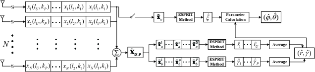
Figure 2: The AoA estimation of the OAM wireless communication system with M-F MT-ESPRIT method

.

To obtain the estimates of $\varphi$ and $\theta$, we have to first build the coordinate system $\textrm{Z}-\textrm{XOY}$ that is at the transmit UCA and parallel to $\bar{\textrm{Z}}-\bar{\textrm{X}}\bar{\textrm{O}}\bar{\textrm{Y}}$, and then get the expression of (II) at $\bar{\textrm{O}}$ point in $\textrm{Z}-\textrm{XOY}$ coordinate system. According to the geometrical model, the angle between $\textrm{Z}^{\prime}$-axis and $\bar{\textrm{Z}}$-axis is $\pi-\theta$, so as Z-axis and $\textrm{Z}^{\prime}$-axis. Let B be a point on the $\textrm{X}^{\prime}$-axis, C is the projection of B on the XOY plane, and D is the projection of C on the X-axis, then $\angle\textrm{BOC}=\theta$. As the lines OC and $\bar{\textrm{O}}\textrm{A}$ are parallel, $\angle\textrm{COD}=\varphi$. Denote the angle between $\textrm{X}^{\prime}$-axis and X-axis as $\gamma$, then $\gamma$ can be obtained as

$$\gamma =\angle\textrm{BOD}=\arccos\left(\cos(\angle\textrm{BOC})\cos(\angle\textrm{COD})\right)$$

$$=\arccos\left(\cos\theta\cos\varphi\right).$$ (2)

Based on (II) and the geometrical model, the electric field intensity at the $m$th $(1\leq m\leq N)$ element of receive UCA in the $\textrm{Z}-\textrm{X}\textrm{O}\textrm{Y}$ coordinate system can be expressed as (I), where $\mathbf{d}_{mn}$ is the position vector from the $n$th transmit antenna element to the $m$th receive antenna element, $\mathbf{\tilde{r}}_{m}=R(\mathbf{\bar{x}}\cos\varphi_{m}+\mathbf{\bar{y}}\sin\varphi_{m})$, $\mathbf{\bar{x}}$ and $\mathbf{\bar{y}}$ are the unit vectors of $\bar{\textrm{X}}$-axis and $\bar{\textrm{Y}}$-axis, $\varphi_{m}=2{\pi}(m-1)/N$, $s(\ell_{u},k_{p})$ is the $\ell_{u}$-th $(-U_{L}\leq\ell_{u}\leq U_{R},U_{L}+U_{R}=U)$ OAM mode information symbol on the $u$th timeslot at frequency $f_{p}=k_{p}c/(2\pi)$ $(1\leq p\leq P)$, $z_{m}(\ell_{u},k_{p})$ is the white Gaussian noise affecting the $\ell_{u}$-th OAM mode at frequency $f_{p}$. Then, all the signals received by the $N$ elements of receive UCA in the $\textrm{Z}-\textrm{X}\textrm{O}\textrm{Y}$ coordinate system are combined, which is expressed as

$$x(\ell_{u},k_{p}) =\sum_{m=1}^{N}x_{m}(\ell_{u},k_{p})$$

$$\approx\beta_{u,p}\frac{e^{ik_{p}r}}{r}e^{i\ell_{u}\gamma}{J_{\ell_{u}}}(k_{p}R\sin\theta){J_{0}}(k_{p}R\sin\theta)$$

$$\quad+z(\ell_{u},k_{p}),$$ (4)

where $\beta_{u,p}=-j\frac{\mu_{0}\omega_{p}dN^{2}}{4\pi}i^{-\ell_{u}}s(\ell_{u},k_{p})$, $z(\ell_{u},k_{p})$ is the corresponding additional noise.

As it happens for multiple-input multiple-output (MIMO) communications, also OAM transmitted frames may carry a combination of training and data symbols. In the case of MIMO, pilot data is used to perform channel estimation, and it is well known that the number of training symbols per subcarrier or subchannel has to be larger than the number of transmit antennas. On the other hand, in the case of OAM, pilot data is exploited for AoA estimation and only $U~{}(1\leq U\leq N)$ training symbols per subcarrier or subchannel are required. Accordingly, we assume that $\{s(\ell_{u},k_{p})|U-L\leq\ell_{u}\leq U_{R},1\leq p\leq P\}$ are the pilot signals in the training phase known to the OAM receiver.

III The AoA Estimation Based on M-F MT-ESPRIT

III-A Problem Formulation

The aim of the AoA estimation is to obtain the estimates of the azimuthal angle $\varphi$ and the elevation angle $\theta$. From (I) and (II), we can observe that the OAM mode number $\ell_{u}$ and the angle $\gamma$ satisfy the dual relationship, so do $k_{p}$ and $r$, where $\gamma=\arccos\left(\cos\theta\cos\varphi\right)$ is an intermediate parameter related to $\varphi$ and $\theta$. Meanwhile, the elevation angle $\theta$ is associated with both $\ell_{u}$ and $k_{p}$. Therefore, we propose to first estimate $r$ and $\gamma$ with the two dual relationships in (II), and then obtain the estimates of $\varphi$ and $\theta$ according to (I). The working process of AoA estimation for multi-mode OAM beams is shown in Fig.2.

III-B Estimation of $r$ and $\gamma$

To estimate $r$ and $\gamma$, we exploit the fact that we can obtain independent estimates of these parameters on each mode $\ell_{u}$ and subcarrier $k_{p}$. Accordingly, at the receiver, we need to extract the exponentials containing $r$ and $\gamma$ from the signal $x(\ell_{u},k_{p})$ by performing the following operation

$$\tilde{x}(\ell_{u},k_{p}) =-\frac{x(\ell_{u},k_{p})}{|x(\ell_{u},k_{p})|}\frac{s^{*}(\ell_{u},k_{p})}{|s(\ell_{u},k_{p})|}i^{\ell_{u}}{\rm sign}(x(\ell_{u},k_{p}))$$

$$=e^{ik_{p}r}e^{i\ell_{u}\gamma}+\tilde{z}(\ell_{u},k_{p}),$$ (5)

where $\tilde{z}(\ell_{u},k_{p})$ is the corresponding noise.

All the signals are received on the $U$ OAM modes at the $P$ frequencies and can be collected in the matrix

$$\mathbf{\tilde{X}}_{U,P}=\begin{bmatrix}\tilde{x}(\ell_{1},k_{1})&\tilde{x}(\ell_{1},k_{2})&\cdots&\tilde{x}(\ell_{1},k_{P})\\ \tilde{x}(\ell_{2},k_{1})&\tilde{x}(\ell_{2},k_{2})&\cdots&\tilde{x}(\ell_{2},k_{P})\\ \vdots&\vdots&\ddots&\vdots\\ \tilde{x}(\ell_{U},k_{1})&\tilde{x}(\ell_{U},k_{2})&\cdots&\tilde{x}(\ell_{U},k_{P})\\ \end{bmatrix}.$$ (6)

For easier analysis, we assume the adopted frequencies and OAM modes satisfy $k_{p+1}-k_{p}=1$ and $\ell_{{u}+1}-\ell_{{u}}=1$.

In the estimation of $r$, we first denote the $u$th row of $\mathbf{\tilde{X}}_{U,P}$ as a column vector $\mathbf{\tilde{x}}_{a}^{u}$, i.e.,

$$\mathbf{\tilde{x}}_{a}^{u}=\mathbf{\tilde{X}}_{U,P}(u,:)=[\tilde{x}(\ell_{u},k_{1}),\tilde{x}(\ell_{u},k_{2}),\cdots,\tilde{x}(\ell_{u},k_{P})]^{\mathrm{T}}.$$

In the ESPRIT-based distance estimation method [7], we can obtain an estimate of $r$ based on the $u$th row of the matrix $\mathbf{\tilde{X}}_{U,P}$, which we denote as $\hat{r}_{u}$. Hence, there are $U$ estimates of $r$ in total, which can be expressed as

$$\hat{r}_{u}= r+\varepsilon_{u},{u}=1,2,\cdots,U,$$

where $\{\varepsilon_{u}|u$$=$$1,2,\cdots,U\}$ represent the estimation errors at $U$ modes. Suppose that $\{\varepsilon_{u}|u=1,2,\cdots,U\}$ have the same average variance $\textrm{Var}(\varepsilon_{r})$, thus,

$$\textrm{Var}\left(\frac{1}{U}\sum_{u=1}^{U}\hat{r}_{u}\right)=\frac{\textrm{Var}\left(\varepsilon_{r}\right)}{U}.$$ (7)

Therefore, $\hat{r}=\frac{1}{U}\sum_{u=1}^{U}\hat{r}_{u}$ is adopted as the estimate of $r$.

In the estimation of $\gamma$, we similarly denote the $p$th column of $\mathbf{\tilde{X}}_{U,P}$ as

$$\mathbf{\tilde{x}}_{b}^{p}=\mathbf{\tilde{X}}_{U,P}(:,p)=[\tilde{x}(\ell_{1},k_{p}),\tilde{x}(\ell_{2},k_{p}),\cdots,\tilde{x}(\ell_{U},k_{p})]^{\mathrm{T}}.$$

After that, by following the same method employed for $\hat{r}$ we can obtain $\hat{\gamma}$, the estimate of $\gamma$.

Algorithm 1 AoA Estimation by M-F MT-ESPRIT Algorithm

Input: $\mathbf{\tilde{X}}_{U,P}$ and $\mathbf{\tilde{x}}_{c}$
  Output: $\varphi$ and $\theta$

1:procedure

2: $\mathbf{\tilde{x}}_{a}^{u}\leftarrow\mathbf{\tilde{X}}_{U,P}(u,:),u=1,2,\cdots,U$

3: $\hat{r}_{u}\leftarrow$ ESPRIT algorithm for $\mathbf{\tilde{x}}_{a}^{u},u=1,2,\cdots,U$

4: $\hat{r}\leftarrow$ $\frac{1}{U}\sum_{u=1}^{U}\hat{r}_{u}$

5: $\mathbf{\tilde{x}}_{b}^{p}\leftarrow\mathbf{\tilde{X}}_{U,P}(:,p),p=1,2,\cdots,P$

6: $\hat{\gamma}_{p}\leftarrow$ ESPRIT algorithm for $\mathbf{\tilde{x}}_{b}^{p},p=1,2,\cdots,P$

7: $\hat{\gamma}\leftarrow$ $\frac{1}{P}\sum_{p=1}^{P}\hat{\gamma}_{p}$

8: $\mathbf{R}_{\mathbf{\tilde{x}}_{c}}\leftarrow\mathbb{E}\left\{\mathbf{\tilde{x}}_{c}{\mathbf{\tilde{x}}_{c}^{\mathrm{H}}}\right\}$

9: Q, $\bm{\Lambda}_{\leftarrow}$ decompose $\mathbf{R}_{\mathbf{\tilde{x}}_{c}}$ such that $\mathbf{Q}\mathbf{\Lambda}\mathbf{Q}^{\mathrm{H}}$$=$$\mathbf{R}_{\mathbf{\tilde{x}}_{c}}$

10: $\lambda_{max}\leftarrow\max\{\lambda_{p}|p=1,2,\cdots,P\}$

11: $\mathbf{q}\leftarrow$the column of Q corresponding to $\lambda_{max}$

12: $\mathbf{q}_{1}$, $\mathbf{q}_{2}\leftarrow$ the first and the last $P-1$ elements of $\mathbf{q}$

13: $e^{i\hat{\xi}}\leftarrow{\mathbf{q}_{1}}^{\dagger}\mathbf{q}_{2}$

14: $\hat{\varphi}\leftarrow\arccos\sqrt{\big{(}\frac{\hat{\xi}-\hat{r}}{R}\big{)}^{2}+\cos{\hat{\gamma}}^{2}}$

15: $\hat{\theta}\leftarrow\arctan\frac{\hat{\xi}-\hat{r}}{R\cos{\hat{\gamma}}}$

16: return $\varphi$ and $\theta$

17:end procedure

III-C Estimation of $\varphi$ and $\theta$

Having estimated $r$ and $\gamma$, we can obtain the azimuth angle $\varphi$ and the elevation angle $\theta$. According to (I), the signal received by the reference element $(\varphi_{1}=0)$ of the receive UCA on the zero OAM mode and $p$th frequency can be simplified as

$$\tilde{x}^{\prime}(k_{p}) =-\frac{x_{1}(0,k_{p})}{|x_{1}(0,k_{p})|}\frac{s^{*}(0,k_{p})}{|s(0,k_{p})|}{\rm sign}(x_{1}(0,k_{p}))$$

$$=e^{ik_{p}\xi}+\tilde{z}^{\prime}(k_{p}),$$ (8)

where $\xi=r+R\sin\theta\cos\varphi$ is an intermediate parameter related to $\varphi$ and $\theta$, $\tilde{z}^{\prime}(k_{p})$ is the corresponding noise.

Then, the signals received on the $P$ frequencies can be collected in the vector

$$\mathbf{\tilde{x}}_{c}=[\tilde{x}^{\prime}(k_{1}),\tilde{x}^{\prime}(k_{2}),\cdots,\tilde{x}^{\prime}(k_{P})]^{\mathrm{T}},$$ (9)

which can be expressed in a compact form as

$$\mathbf{\tilde{x}}_{c}=\mathbf{c}+\mathbf{z}_{c},$$ (10)

where $\mathbf{c}$ $=$ $[e^{ik_{1}\xi},e^{ik_{2}\xi},\cdots,e^{ik_{P}\xi}]^{T}$ and $\mathbf{z}_{c}$ is the corresponding noise vector.

The covariance matrix of $\mathbf{\tilde{x}}_{c}$ can be written as

$$\mathbf{R}_{\mathbf{\tilde{x}}_{c}}=\mathbb{E}\left\{\mathbf{\tilde{x}}_{c}{\mathbf{\tilde{x}}_{c}}^{H}\right\}=\mathbf{c}\mathbf{c}^{H}+\mathbf{R}_{\mathbf{z}_{c}},$$ (11)

where $\mathbf{R}_{\mathbf{z}_{c}}=\mathbb{E}\left\{\mathbf{z}_{c}{\mathbf{z}_{c}}^{\mathrm{H}}\right\}$. The eigenvalue decomposition (EVD) of $\mathbf{R}_{\mathbf{\tilde{x}}_{c}}$ is

$$\mathbf{R}_{\mathbf{\tilde{x}}_{c}}=\mathbf{Q}\mathbf{\Lambda}\mathbf{Q}^{H},$$ (12)

where $\mathbf{Q}$ is an $P\times P$ unitary matrix and $\mathbf{\Lambda}=\textrm{diag}\{\lambda_{1},$ $\lambda_{2},\cdots,\lambda_{P}\}$. Denote as $\lambda_{max}=\max\{\lambda_{p}|p=1,2,\cdots,P\}$, and as $\mathbf{q}$ the eigenvector corresponding to $\lambda_{max}$, so that it is

$$\mathbf{R}_{\mathbf{\tilde{x}}_{c}}\mathbf{q}=\lambda_{max}\mathbf{q}.$$ (13)

Now, the subspace spanned by $\mathbf{q}$ is the signal subspace spanned by $\mathbf{c}$ so that the following relationship holds true

$$\mathbf{c}=\textrm{T}\mathbf{q},$$ (14)

where T is a non-zero parameter. If we consider the two vectors $\mathbf{c}_{1}$ and $\mathbf{c}_{2}$, obtained by taking the first and the last $P-1$ elements of $\mathbf{c}$, respectively, it is $\mathbf{c}_{2}={\Phi}\mathbf{c}_{1}$, where $\Phi=e^{i\xi}$. To obtain the estimate of $\xi$, we construct the two vectors $\mathbf{q}_{1}$ and $\mathbf{q}_{2}$, composed by the first and by the last $P-1$ elements of $\mathbf{q}$, respectively. Then, exploiting the fact that $\mathbf{c}_{1}=\textrm{T}\mathbf{q}_{1}$ and $\mathbf{c}_{2}=\textrm{T}\mathbf{q}_{2}$, one obtains

$$\mathbf{q}_{2}={\Phi}\mathbf{q}_{1},$$ (15)

which leads to

$$e^{i\hat{\xi}}={\mathbf{q}_{1}}^{\dagger}\mathbf{q}_{2},$$ (16)

where $\hat{\xi}$ is the estimate of $\xi$ based on the signal vector $\mathbf{\tilde{x}}_{c}$.

After that, according to

$$\hat{\varphi}=\arccos\sqrt{\big{(}\frac{\hat{\xi}-\hat{r}}{R}\big{)}^{2}+\cos{\hat{\gamma}}^{2}},$$

$$\hat{\theta}=\arctan\frac{\hat{\xi}-\hat{r}}{R\cos{\hat{\gamma}}},$$ (17)

the estimates of the azimuthal angle $\varphi$ and the elevation angle $\theta$ can be obtained. Thus, the AoA estimation by M-F MT-ESPRIT algorithm is completed, and the detailed procedure is summarized in Algorithm 1. Compared with the existing AoA estimation method [7], the AoA estimation method based on M-F MT-ESPRIT algorithm can estimate the azimuth and elevation angles of muiti-mode OAM beams only by utilizing the exponentials of the received training signals, which is easier to implement in practical applications.

TABLE I: The complexity of the AoA estimation.

Procedure	Complexity
Estimating $\hat{r}$	$\mathcal{O}\left(UP^{\max\{2,g\}}\right)$
Estimating $\hat{\gamma}$	$\qquad\quad\mathcal{O}\left(PU^{\max\{2,g\}}\right)$
Eq.$(11):\mathbf{R}_{\mathbf{\tilde{x}}_{c}}=\mathbb{E}\left\{\mathbf{\tilde{x}}_{c}{\mathbf{\tilde{x}}_{c}}^{H}\right\}$	$\qquad\qquad\quad\mathcal{O}\left(P^{2}\right)$
Eq.$(12):\mathbf{R}_{\mathbf{\tilde{x}}_{c}}=\mathbf{Q}\mathbf{\Lambda}\mathbf{Q}^{H}$	$\qquad\qquad\quad\mathcal{O}\left(P^{g}\right)$
Eq.$(16):e^{i\hat{r}_{u}}={\mathbf{q}^{1}_{u}}^{\dagger}\mathbf{q}^{2}_{u}$	$\qquad\qquad\quad\mathcal{O}\left(P\right)$
The total complexity: $\mathcal{O}\left(UP^{\max\{2,g\}}\right)+\mathcal{O}\left(PU^{\max\{2,g\}}\right)$

The computational complexities of the proposed AoA estimation method based on M-F MT-ESPRIT algorithm is summarized in Table LABEL:Table1, where $g$ is generally equal to 3, but can be reduced to 2.376 when the Coppersmith and Winograd algorithm [13] is applied to the eigenvalue decomposition in (12). Due to the use of M-F MT-ESPRIT algorithm, the dimension of the training signal vector processed by ESPRIT algorithm each time is greatly reduced. The total complexity comparison between the existing AoA estimation method [7] and the proposed AoA estimation method based on M-F MT-ESPRIT algorithm is shown in Fig.3.

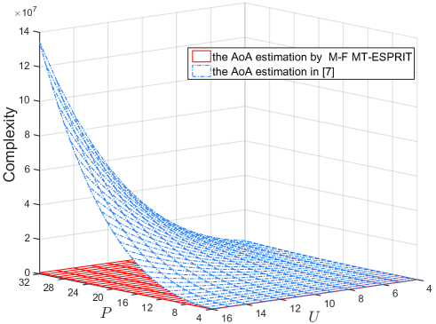
Figure 3: The complexities of the AoA estimation method based on M-F MT-ESPRIT algorithm and the AoA estimation method in [7] vs. $P$ and $U$ with $g=3$.

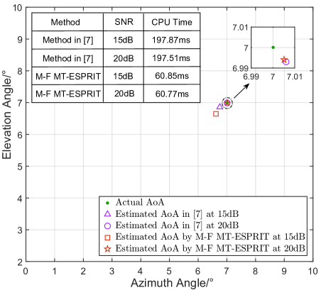
Figure 4: The AoA estimation results at 15dB and 20dB.

IV Simulation Results and Performance Analysis

We first verify the proposed AoA estimation method by numerical simulations, and then compare the accuracy of the AoA estimation method proposed in this paper with that proposed in [7]. Thereafter, we compare the capacity performance of the OAM channel without beam steering and that with beam steering [7] based on the estimated AoA. In the simulation, we choose $N=9$, $P=8$ subcarriers from 2.244GHz to 2.578GHz corresponding to the wave number $k_{p}=47,48,\dots,54$, number of OAM modes $U=8$ with $\ell_{u}=-4,-3,\cdots,+3$, $R=10\lambda_{1}$, $\lambda_{1}=2\pi/k_{1}$, $(r,\varphi,\theta)=(40\textrm{m},7^{\circ},7^{\circ})$. Besides, we assume the angle range of receive UCA’s main lobe $[\alpha_{a},\alpha_{b}]=[2^{\circ},8^{\circ}]$, the initial number of intervals $\mathcal{D}=2$ [7]. Unless otherwise stated, the SNRs in all the figures are defined as the ratio of the received signal power versus the noise power.

The AoA estimation results of the proposed M-F MT-ESPRIT method and the method proposed in [7] are shown in Fig. 4. It can be seen from the figure that with the increase of SNR the estimated AoAs approach to the actual value. When SNR$=20$dB, the AoA estimated by M-F MT-ESPRIT method is $(\hat{\varphi},\hat{\theta})=(7.005^{\circ},6.994^{\circ})$, and the AoA estimated by the method in [7] is $(\hat{\varphi},\hat{\theta})=(7.006^{\circ},6.993^{\circ})$, which are very close to the actual AoA. Besides, the CPU time of M-F MT-ESPRIT method is much lower than that of the method in [7].

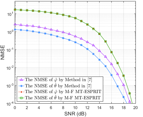
Figure 5: The NMSEs of the estimated $\hat{\varphi}$ and $\hat{\theta}$ vs. SNR.

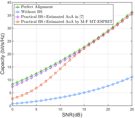
Figure 6: The capacity comparison of the OAM channel with perfect alignment, without BS, with BS by the estimated AoA in this paper, and with BS by the estimated AoA in [7]. BS: beam steering.

Fig.5 illustrates the normalized mean-squared errors (NMSEs) of $\hat{\varphi}$ and $\hat{\theta}$ obtained by M-F MT-ESPRIT method and the method in [7]. The NMSE is defined as $\mathbb{E}\{(\hat{x}-x)^{2}/x^{2}\}$, where $\hat{x}$ denotes the estimate of $x$. For the proposed M-F MT-ESPRIT method, as SNR increases the NMSEs of $\hat{\varphi}$ and $\hat{\theta}$ decline. It follows that the proposed M-F MT-ESPRIT method is able to accurately estimate the AoA of multi-mode OAM beams. Moreover, due to the reduction of the dimension of the training signal vector processed by ESPRIT algorithm each time, the NMSEs of $\hat{\varphi}$ and $\hat{\theta}$ obtained by M-F MT-ESPRIT method is higher than those obtained by the method in [7].

In Fig.6, we compare the capacity of the OAM channel with perfect alignment, without beam steering, with beam steering by the estimated AoA in this paper, and with beam steering by the estimated AoA in [7]. The capacity of the misaligned OAM channel is greatly improved and approaches the capacity of accurately aligned OAM channel after applying the beam steering with the AoA estimation method proposed in this paper and in [7]. Therefore, the accurate AoA estimation is essential for the OAM receiver to improve the capacity of the misaligned OAM channel. Moreover, due to the larger estimation error of $\hat{\varphi}$ and $\hat{\theta}$, the capacity of the OAM channel with beam steering by the estimated AoA in this paper is lower than that by the estimated AoA in [7] under the low SNRs.

V Conclusions

In this paper, an AoA estimation method based on M-F MT-ESPRIT algorithm for OAM wireless communication systems is proposed, which can accurately estimate the azimuth and elevation angles of multi-mode OAM beams only based on the received training signals. With the accurately estimated AoA, the capacity of the misaligned OAM channel can be greatly improved by beam steering and approaches the capacity of accurately aligned OAM channel. Moreover, compared with the existing AoA estimation method [7], the total complexity of the proposed AoA estimation method based on M-F MT-ESPRIT algorithm is significantly decreased, which is more practical.

References

• [1] L. Allen, M. Beijersbergen, R. Spreeuw, and J. Woerdman, “Orbital angular momentum of light and the transformation of laguerre-gaussian laser modes,” Physical Review A, vol. 45, no. 11, p. 8185, 1992.
• [2] R. Chen, H. Zhou, M. Moretti, X. Wang, and J. Li, “Orbital angular momentum waves: generation, detection, and emerging applications,” IEEE Commun. Surveys Tuts., vol. 22, no. 2, pp. 840–868, 2020.
• [3] Y. Yan, G. Xie, M. P. J. Lavery, H. Huang, N. Ahmed, C. Bao, Y. Ren, Y. Cao, L. Li, Z. Zhao, A. F. Molisch, M. Tur, M. J. Padgett, and A. E. Willner, “High-capacity millimetre-wave communications with orbital angular momentum multiplexing,” Nat. Commun., vol. 5, p. 4876, 2014.
• [4] R. Chen, W. Yang, H. Xu, and J. Li, “A 2-D FFT-based transceiver architecture for OAM-OFDM systems with UCA antennas,” IEEE Trans. Veh. Technol., vol. 67, no. 6, pp. 5481–5485, Jun. 2018.
• [5] W. Cheng, W. Zhang, H. Jing, S. Gao, and H. Zhang, “Orbital angular momentum for wireless communications,” IEEE Wireless Commun., vol. 26, no. 1, pp. 100–107, Feb. 2019.
• [6] R. Chen, H. Xu, X. Wang, and J. Li, “On the performance of OAM in keyhole channels,” IEEE Wireless Commun. Lett., vol. 8, no. 1, pp. 313–316, Feb. 2019.
• [7] R. Chen, W. Long, X. Wang, and J. Li, “Multi-mode OAM radio waves: generation, angle of arrival estimation and reception with UCAs,” IEEE Trans. Wireless Commun., vol. 19, no. 10, pp. 6932–6947, 2020.
• [8] R. Chen, H. Xu, M. Moretti, and J. Li, “Beam steering for the misalignment in UCA-based OAM communication systems,” IEEE Wireless Commun. Lett., vol. 7, no. 4, pp. 582–585, Aug. 2018.
• [9] X. P. Wang, L. Y. Wang, X. M. Li, and G. Bi, “Nuclear norm minimization framework for DOA estimation in MIMO radar,” Signal Processing, vol. 135, pp. 147–152, 2017.
• [10] F. Wen, Z. Zhang, K. Wang, G. Sheng, and G. Zhang, “Angle estimation and mutual coupling self-calibration for ULA-based bistatic MIMO radar,” Signal Processing, vol. 144, pp. 61–67, 2018.
• [11] L. Wan, X. Kong, and F. Xia, “Joint range-doppler-angle estimation for intelligent tracking of moving aerial targets,” IEEE Internet Things J., vol. 5, no. 3, pp. 1625–1636, 2018.
• [12] S. M. Mohammadi, L. K. S. Daldorff, J. E. S. Bergman, R. L. Karlsson, B. Thide, K. Forozesh, T. D. Carozzi, and B. Isham, “Orbital angular momentum in radio-a system study,” IEEE Trans. Antennas Propa., vol. 58, no. 2, pp. 565–572, Feb. 2010.
• [13] V. Y. Pan and Z. Q. Chen, “The complexity of the matrix eigenproblem,” in Proceedings of the thirty-first annual ACM symposium on Theory of computing, 1999, pp. 507–516.