Impact of biaxial birefringence in polar ice at radio frequencies on signal polarizations in ultra-high energy neutrino detection

Abstract

It is known that polar ice is birefringent and that this can have implications for in-ice radio detection of ultra-high energy neutrinos. Previous investigations of the effects of birefringence on the propagation of radio-frequency signals in ice have found that it can cause time delays between pulses in different polarizations in in-ice neutrino experiments, and can have polarization-dependent effects on power in radar echoes at oblique angles in polar ice. I report, for the first time, on implications for the received power in different polarizations in high energy neutrino experiments, where the source of the emitted signal is in the ice, a biaxial treatment at radio wavelengths is used, and the signals propagate at oblique angles. I describe a model for this and compare with published results from the SPICE in-ice calibration pulser system at South Pole, where unexpectedly high cross-polarization power has been reported for some geometries. The data shows behaviors indicative of the need for a biaxial treatment of birefringence inducing non-trivial rotations of the signal polarization. The behaviors include, but are not limited to, a time delay that would leave an imprint in the power spectrum. I explain why this time delay has the potential to serve as both an in-ice neutrino signature and a measurement of the distance to the interaction. While further work is needed, I expect that proper handling of the effects presented here will increase the science potential of ultra-high energy neutrino experiments, and may impact the optimal designs of next-generation detectors.

I Introduction

Ultra-high energy neutrinos are a crucial missing piece in the rapidly expanding field of multi-messenger astrophysics [1, 2, 3]. Alongside the mature and evolving measurements of cosmic rays and gamma rays up to their highest detectable energies, the past decade has seen the discovery of a high energy astrophysical neutrino flux up to O(10) PeV [4, 5, 6], as well as the first gravitational wave detections [7, 8]. Ultra-high energy neutrinos ($>10^{17}$ eV) will be unique messengers to the most powerful astrophysical processes at cosmic distances [9] and unique probes of fundamental physics at extreme energies [10, 11, 12].

Polar ice sheets are being utilized by many experiments as a detection medium for high-energy astrophysical neutrinos [13, 14, 15], including many that are designed to detect neutrinos via a broadband “Askaryan” radio impulse [16, 17, 18, 19, 20, 21]. So far no neutrinos have been detected with radio techniques. Due to the transparency of pure ice at radio frequencies, the neutrino-induced signals will have propagation distances of order kilometers in the ice before being detected by antennas either from within or above the ice. Thus, it is important to understand the impact of the ice on the properties of signals as they propagate over that distance scale. Ice crystals are known to be birefringent and in some locations it has been shown that polar ice can be treated as biaxial at radio frequencies [22]. This comes about because there are two special directions in the ice: the direction of ice flow, which is in the horizontal plane, and the vertical direction due to compression.

Previous studies have investigated properties of polar ice and their impact on the detection of neutrino-induced radio impulses using diverse datasets and detailed simulations. Radio-frequency measurements in polar ice have characterized the depth-dependent indices of refraction $n(z)$ and the attenuation of signal power at radio frequencies  [23, 24, 18, 25]. That $n(z)$ is not constant can bring about two solutions for rays propagating between source and receiver called direct and reflected/refracted, and both have been observed. Simulation studies have stressed the importance of using techniques beyond simple ray tracing to model signal propagation, especially in non-uniform ice  [26, 27]. In Ref. [28], previously unanticipated modes of horizontal propagation in the ice were reported. Ref. [29] reported evidence of birefringence in the ice sheet as seen in delays between signals of different polarizations using bistatic radar from the surface.

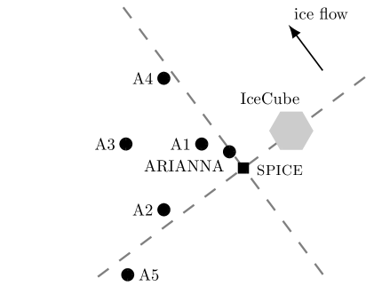
Figure 1: Layout of the SPICE core, the five ARA stations, the ARIANNA South Pole station, and IceCube in the northing-easting coordinate system. The arrow shows the direction of ice flow, and the dashed gray lines intersect the location of the SPICE core and are parallel to and perpendicular to ice flow.

The South Pole Ice Core Experiment (SPICE) calibration system has provided a unique dataset to study the impulsive signals with the transmitters, propagation over ${\sim}{\rm km}$-scales, and receivers all being within the ice. As seen in Fig. 1, the ARA and ARIANNA in-ice neutrino experiments embedded in the ice measured radio-frequency impulses up to 4 km away from their source. Five ARA stations (A1-A5) observed the pulses from 100 to 200 m depths, and two ARIANNA stations from just below the surface.

In Ref. [30], using SPICE pulse measurements, ARA reported bounds on the depth-dependent index of refraction at South Pole, time differences between signals detected in different polarizations due to birefringence, and attenuation lengths for horizontally propagating signals. ARIANNA reported measurements of the polarization of signals from a SPICE transmitter after propagating ${\sim}1$ km distance in the ice [31]. Jordan et al. [32] utilized ice fabric properties from the SPICE ice core to predict time differences between signals in different polarizations that were consistent with observations using a biaxial birefringence treatment for near-horizontal propagation and restricted to special cases. Besson et al. [33] extended this work to vertical propagation and additionally used past data from the RICE experiment.

ARA and ARIANNA both observed strange effects in the polarization of SPICE pulses when viewing them at different geometries [31, 30]. First, while SPICE pulses were transmitted predominantly in one polarization, they were often observed with larger-than-expected power in the other (cross-) polarization. Sometimes even more power was observed in the cross-polarization than in the transmitted polarization. Second, the dependence of the observed signal polarization on receiver positions and viewing angles did not follow clear patterns. Similar effects have also been reported in earlier measurements of radio signals in polar ice after long propagation distances in Ref. [34]. In this paper, I propose that birefringence that is effectively biaxial at radio frequencies in the ice is a plausible explanation for these effects, outlining a model to predict signal polarizations with transmitter and receiver both in the ice, and compare against already reported observations of SPICE pulses.

Outside of radio neutrino detection, others have investigated the impact of birefringence on signal propagation in ice. Recently the IceCube neutrino telescope at South Pole, which detects optical Cerenkov light from neutrinos in the ice, has reported an anisotropic attenuation and attributes it to birefringence [35, 36]. Since optical wavelengths are much shorter than few-mm individual crystal sizes, they propagate light through uniaxial ice crystals whose orientations are distributed as expected in the ice and that have been elongated due to ice flow and refract the light across boundaries between crystals. In recent years there has been much development in radar polarimetry, which assesses the impact of the birefringence properties of the ice on return power and polarization [37, 22, 38, 39, 40, 41, 42, 43, 44, 45, 46, 47] in radar measurements.

This paper is organized as follows. First, I give a big picture overview of the core concepts behind this paper. Then, I briefly summarize the already established theory behind the propagation of electromagnetic radiation in biaxially birefringent crystals. Next, I describe the SPICE calibration campaign and the ARA and ARIANNA detectors at South Pole. In the next section, I predict the behavior of received signal spectra and power measured in different polarizations in the ARA and ARIANNA stations after signal propagation while treating the ice sheet as biaxially birefringent and then compare with published results. Finally, I conclude with implications for experiments using radio techniques to search for neutrinos in polar ice.

II Overview of the core concepts in this paper

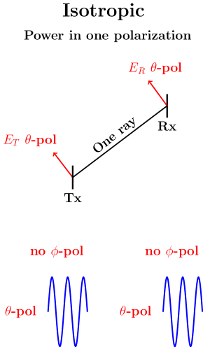
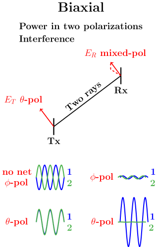
Figure 2: Illustration of a pure $\theta$-pol signal (no cross-pol) emitted by a transmitter (Tx) in the ice and propagated to the position of a receiver (Rx) at a more shallow depth. Here, $\theta$-pol is the polarization in the plane of the page and perpendicular to the ray, and $\phi$-pol is into the page. Although this figure is only meant to serve as an illustration, it is modeled after a 300 MHz signal transmitted from the SPICE pulser at 1000 m and received by an A1 station at 100 m depth (more details of the stations in Sec. IV). (Left) In the case of an isotropic medium, there is one direct ray and a pure $\theta$-pol signal remains purely $\theta$-pol at the receiver. (Right) In a birefringent medium, there are two direct rays. Since here the signal is purely $\theta$-pol, the $\phi$-pol components are such that they cancel each other. During propagation, in a biaxially birefringent medium, each ray’s envelope power can have its mixture of polarizations altered, and the two rays can also interfere. Both effects contribute to a mixed polarization of the signal at the receiver.

Fig. 2 illustrates the main points underlying what I present in this paper. I address, for the first time, the impact that birefringence that is effectively biaxial will have on the power received by antennas measuring different polarizations in in-ice radio neutrino experiments with the transmitter-receiver system fully embedded in the ice. I compare expectations with previously reported measurements of SPICE pulses.

In an isotropic medium (left panel of Fig. 2), a signal transmitted in one polarization is received in the same polarization and there is one direct path taken by a single ray between transmitter and receiver. Throughout this paper, a “ray” is defined by a path running tangent to its wave vector ${\bf k}$ and has a unique displacement vector ${\bf D}$ and electric field ${\bf E}$ associated with it at any given time. Also, $\theta$-pol is the polarization in the plane of the page and perpendicular to ${\bf k}$, and $\phi$-pol is into the page.

The right panel of Fig. 2 illustrates the effects considered in this paper that biaxial birefringence can have on the polarization of signals. I consider two rays along the same direct path (always with the same ${\bf k}$ between them), but each ray has its own ${\bf D}$ and electric field ${\bf E}$. Here the signal is transmitted in the $\theta$-pol polarization in a birefringent medium that is effectively biaxial, and so the $\phi$-pol components from the two rays cancel one another.

Two different effects can cause the polarization observed at the receiver to be different from the one transmitted as seen in Fig. 2. First, the polarization of each ray will change along its path for two reasons: the properties of the birefringent crystal are depth-dependent, and the ray’s direction (the direction of ${\bf k}$) changes with respect to the crystal axes due to the depth-dependent index of refraction. This is illustrated in Fig. 2 as the same ray having different polarization components at the transmitter and receiver. Second, in each polarization, the electric fields associated with the two rays will interfere. This is illustrated as the two rays having a relative delay at the receiver in either polarization. Both of these effects will impact the polarization of the signal detected at the receivers. I note that in a birefringent medium, two rays may further split along their path into more rays, but I neglect this and only consider the two rays that leave the transmitter.

In this paper, I lay out the effect of a biaxial treatment of birefringence on long-distance propagation with the source and transmitter both in the ice, and to this aim, I make a few simplifications. First, only a single frequency is ever propagated at a time. Second, while I use a depth-dependent index of refraction, I only consider the direct solution between the transmitter and receiver and neglect the reflected/refracted solution that is often present. Third, I consider only two rays, without allowing for any further splitting of rays along the path. This is justified by the observation of SPICE pulses that remain impulsive at the receivers with a single time delay between pulses in the two polarizations [30]. Fourth, I take the power in each ray to be constant along their path. So, the power in ray 1 at the transmitter stays in ray 1 even as the polarization of ray 1 rotates along the path, and the same for ray 2. This appears to be also the approach taken in Ref. [22]. Finally, I take the direct path to be the same for the two rays (both rays will have the same ${\bf k}$ at any time), while other properties of the ray (${\bf D}$, ${\bf E}$, and Poynting vector ${\bf S}$) will all be different between the two rays. It will be important to consider the more general cases in future work.

The formalism presented here for signal propagation in ice using a biaxial treatment of birefringence appears to be consistent with the one laid out for radar returns at oblique angles in Matsuoka et al. [22], and the one in Fujita et al. [39] for vertical propagation. However, unlike both of those, I do not include any loss of power due to scattering.

Scattering would only have an important impact on this paper if it were anisotropic, and only if it is large enough to impact the transmitted power. Ref. [22] reports that from radar data in Antarctica, anisotropies in backscattered power can at most change the return power by about 10-15 dB [37, 48], and so for a typical return power of -80 to -60 dB, it only affects the transmitted power at typically at the -60 dB level (one part in a million).

III Background on birefringence

A birefringent crystal is an anisotropic medium, meaning that the propagation of electromagnetic radiation depends on its direction and polarization due to a distinctive feature of one or more axes within the crystal. An anisotropic medium may exhibit a symmetry about one axis, in which case it is uniaxially birefringent and is characterized by two parameters. Biaxial birefringent crystals are characterized by three parameters along three perpendicular axes.

While individual ice crystals are uniaxially birefringent, at radio frequencies the electromagnetic properties of the ice depend on both the birefringence of the individual crystals and the distribution of crystal orientations, known as the crystal orientation fabric (COF) within the ice volume (the bulk)  [49]. At radio frequencies, the $\mathcal{O}$(1 m) wavelengths are much larger than the typical $\mathcal{O}$(a few mm)-sized crystals in polar ice [50].

Ice Ih is the form of ice found in ordinary water that has been frozen at atmospheric pressure, or has been formed directly from water vapor at $>100\,^{o}$ C [51]. An Ice Ih crystal consists of stacked planes of H₂O molecules that form a hexagonal structure in each plane, with the hexagons in neighboring planes aligned. The oxygens sit at the vertices of hexagons, and hydrogen forms bonds with neighboring oxygens to connect the lattice.

The hexagonal structure of Ice Ih crystals leads to the axial symmetry that gives rise to uniaxial birefringence. Here, as in [22], I model the ice as a biaxially birefringent crystal even though it is composed of uniaxially birefringent crystals. This is motivated by the crystal orientations being influenced by two special axes: 1) the vertical axis, due to compression and 2) the direction of the flow of ice, which is in the horizontal plane.

In this section, I provide the reader with the basics behind electromagnetic waves in biaxially birefringent media and then outline how I apply that theory to the case of transmitting and receiving radio frequency (RF) signals in South Pole ice. I refer the reader to Refs. [52, 53, 54, 55, 56, 57, 58, 59, 60] for more complete treatments. There are many places where I refer to a vector without the hat, even when only the direction is needed, to simplify notation. I do use the hat when it is necessary for units.

III.1 Electromagnetism in biaxially birefringent crystals

In a biaxially birefringent crystal, for a given wave vector ${\bf k}$, there are not one but two “rays,” and each propagates with a different index of refraction. Those two rays have displacement vectors ${\bf D_{1}}$ and ${\bf D_{2}}$ that are perpendicular to one another. As in isotropic media, the displacement vectors sit in the plane perpendicular to ${\bf k}$.

To find ${\bf D_{1}}$ and ${\bf D_{2}}$ for a given ${\bf k}$, it is useful to think of the wavefront encountering three parameters $n_{\alpha}$, $n_{\beta}$, and $n_{\gamma}$, which are properties of the medium, and at South Pole are depth-dependent (see Fig. 3). These parameters form the three perpendicular semi-axes of an ellipsoid called an “indicatrix,” and here the $\alpha$- and $\gamma$-axes are taken to be aligned with ice flow and the compression, respectively. The semi-axes are also called principal axes. Although they are indices of refraction, we will see that a ray only propagates with its indices of refraction equal to $n_{\alpha}$, $n_{\beta}$, or $n_{\gamma}$ in special cases. For an isotropic medium, $n_{\alpha}=n_{\beta}=n_{\gamma}$, for a uniaxially birefringent medium two semi-axes are the same, and for a biaxially birefringent medium such as we treat South Pole ice in this paper they are all different, and by convention, $n_{\alpha}<n_{\beta}<n_{\gamma}$.

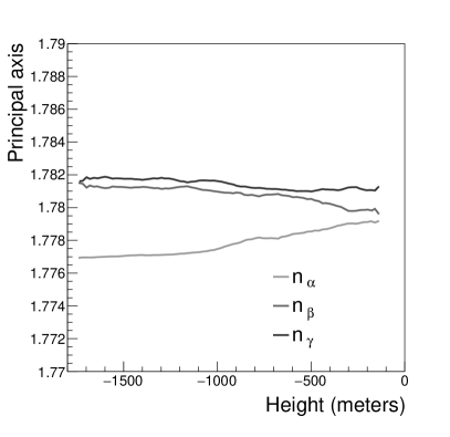
Figure 3: (Left) Principal indices of refraction used in this paper as reported by Voigt [61] and also utilized in [32]. For the work in this paper, I smooth the data with a three-point running average. (Right) Illustration of an indicatrix with dimensions exaggerated compared to what is observed in South Pole ice. An ellipse is shown that represents the intersection of a planar wavefront for an incident wave vector ${\bf k}$ with the indicatrix. The eigenvectors of the displacement vector ${\bf D}$ are the major and minor axes of that ellipse of intersection.

Now we can find the directions of ${\bf D_{1}}$ and ${\bf D_{2}}$ given ${\bf k}$, $n_{\alpha}$, $n_{\beta}$, and $n_{\gamma}$. The intersection of the planar wavefront, which is perpendicular to ${\bf k}$, with the indicatrix forms an ellipse. The directions of ${\bf D_{1}}$ and ${\bf D_{2}}$ are then in the directions of the major and minor axes of that ellipse, and the lengths of the major and minor axes are the indices of refraction seen by the two rays.

The direction of the electric fields ${\bf E_{1}}$ and ${\bf E_{2}}$ associated with the two rays are related to ${\bf D_{1}}$ and ${\bf D_{2}}$ using an equation of a familiar form:

$${\bf D_{1,2}}={\bm{\varepsilon}}{\bf E_{1,2}}.$$ (1)

While in isotropic media they would be related by a scalar $\varepsilon$, in birefringent media, ${\bm{\varepsilon}}$ is a tensor given by:

$$\begin{bmatrix}n_{\alpha}^{2}&0&0\\ 0&n_{\beta}^{2}&0\\ 0&0&n_{\gamma}^{2}\\ \end{bmatrix}.$$ (2)

This means that ${\bf D}$ is not in general parallel to ${\bf E}$, though at South Pole they are within a fraction of a degree. Recalling that ${\bf k}$ is perpendicular to ${\bf D}$, then ${\bf k}$ is in general not perpendicular to ${\bf E}$. The electric fields ${\bf E_{1}}$ and ${\bf E_{2}}$ are perpendicular to one another.

Considering the first ray, ${\bf k}$, ${\bf E_{1}}$, and ${\bf D_{1}}$ are all related by the wave equation, which now has an extra term compared to the more familiar form due to ${\bf E}$ not being perpendicular to ${\bf k}$:

$$(-{\bf k}\cdot{\bf k}){\bf E_{1}}+({\bf k}\cdot{\bf E_{1}}){\bf k}=-\mu_{0}\omega^{2}{\bm{\varepsilon}}{\bf E_{1}}.$$ (3)

Recall that on the right side of the equation, ${\bm{\varepsilon}}{\bf E_{1}}={\bf D_{1}}$. Here, $\mu_{0}$ is the usual permeability constant and $\omega$ is the angular frequency of the wave. This equation of course also must be satisfied with ${\bf E_{1}}\rightarrow{\bf E_{2}}$, and ${\bf D_{1}}\rightarrow{\bf D_{2}}$. The displacement vectors ${\bf D_{1}}$ and ${\bf D_{2}}$ corresponding to a given ${\bf k}$ are the two eigenvectors of this wave equation and the indices of refraction seen by each ray are the corresponding eigenvalues.

In biaxially birefringent media, the Poynting vector ${\bf S}$ points in the direction of energy flow, just as in isotropic media, but now for a given ${\bf k}$, there are two Poynting vector directions, ${\bf S_{1}}$ and ${\bf S_{2}}$, one for each of the two rays, and neither is in general parallel to ${\bf k}$. These are found from the usual relationship:

$${\bf S_{1,2}}={\bf E_{1,2}}\times{\bf H}.$$ (4)

Here, the direction of ${\bf H}$ can be found by crossing ${\bf k}$ into ${\bf D}$:

$${\bf\hat{H}_{1,2}}={\bf\hat{k}_{1,2}}\times{\bf\hat{D}_{1,2}}.$$ (5)

III.2 The $\epsilon$ angles

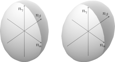
Figure 4: These two ellipsoids are not the same and will be used in Fig. 5 to demonstrate the reason that a biaxial treatment of birefringence is needed for the $\epsilon$ angles to be non-zero. (Left) Indicatrix for a uniaxial crystal (here, $n_{\alpha}=n_{\beta}=1.0$, $n_{\gamma}=1.5$), and (Right) indicatrix for a biaxial crystal (here, $n_{\alpha}=1.0$, $n_{\beta}=1.3$, $n_{\gamma}=1.5$). I take indicatrices with features exaggerated compared to those observed in the ice for illustration purposes.

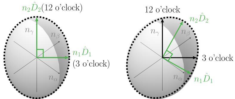
Figure 5: These are the same two ellipsoids as the ones shown in Fig. 4. (Left) Indicatrix for a uniaxial crystal, and (Right) indicatrix for a biaxial crystal. Consider ${\bf k}$ for an incident ray to be into the page, where it hits indicatrix at oblique angles (here, $\theta=45^{\circ}$, $\phi=45^{\circ}$ in a usual spherical coordinate system). The planar wavefront is in the plane of the page. The outline of the shaded region shown as the dashed black line is the intersection ellipse, that is, the intersection of the planar wavefront with the ellipsoid. The axes of the ellipse are the eigenvectors of ${\bf D}$. For the uniaxial crystal, the eigenvectors are at 12 o’clock and 3 o’clock as seen by an observer looking along ${\bf k}$, and for the biaxial crystal, the eigenvectors are rotated by an angle in the plane of the page with respect to 12 o’clock and 3 o’clock.

In this paper, I highlight two problems seen in the data and describe how a biaxial treatment of birefringence in the ice may explain them: 1) detecting power in $\phi$-type antennas after transmitting from a $\theta$-type antenna and 2) the complicated dependencies between the relative power in $\phi$-type and $\theta$-type antennas and the positioning of the transmitter relative to the receiver. I introduce angles that I call $\epsilon$ that I view as being at the core of the emergence of these effects. The $\epsilon$ angles also point to a biaxial treatment of birefringence being needed to bring about the behaviors seen in the data, as they would not be present in either a uniaxially birefringent or isotropic medium. I note that $\epsilon$ is referred to as $\varphi$ in Matsuoka et al. [22].

We will consider a biaxially birefringent crystal and a uniaxial one, shown in Fig. 4, and compare their effect on the eigenvectors of ${\bf D}$, and thus the orientation of the electric fields. For illustration purposes, the differences between semi-axes are exaggerated in this figure compared to what is expected in the ice. In this section, for the uniaxial crystal I take $n_{\alpha}=n_{\beta}=1.0$ and $n_{\gamma}=1.5$, and for the biaxially birefringent crystal I take $n_{\alpha}=1.0$, $n_{\beta}=1.3$, and $n_{\gamma}=1.5$.

Recall that for a given ${\bf k}$, there are two eigenvectors for ${\bf D}$. The planar wavefront is perpendicular to ${\bf k}$. The directions of the eigenvectors of ${\bf D}$ are along the major and minor axes of the ellipse defined by the intersection of the planar wavefront and the indicatrix.

Fig. 5 illustrates the effect that these two types of crystals have on the orientations of the eigenvectors of ${\bf D}$. On each side of the figure, consider ${\bf k}$ to be approaching the indicatrix into the page and perpendicular to the page. On the left side of the figure, when ${\bf k}$ is incident on the uniaxial indicatrix, there is a symmetry about the $\gamma$-axis, and to an observer looking in the direction of ${\bf k}$, the axes of the intersection ellipse will appear to sit at 12 o‘clock and 3 o‘clock. What I call 12 o‘clock is the direction that is perpendicular to ${\bf k}$ and in the plane of ${\bf k}$ and the $\gamma$-axis. On the right side of the figure, when ${\bf k}$ is incident on a biaxial crystal, the symmetry is lost, and the eigenvectors of ${\bf D}$ will, in general, be rotated with respect to 12 o‘clock and 3 o‘clock by an angle.

The angles that the ${\bf D}$ eigenvectors make with the 12 o’clock and 3 o’clock directions are almost what I call the $\epsilon$ angles but not quite, because polarizations are in the directions of the corresponding electric fields ${\bf E_{1,2}}$ for the two eigensolutions. Recall that ${\bf E}$ and ${\bf D}$ are not in the same direction although they are within a fraction of a degree of one another. The electric fields are perpendicular to the directions of the Poynting vectors ${\bf S_{1}}$ and ${\bf S_{2}}$, not ${\bf k}$, and the latter three are not in the same direction, but are also within a fraction of a degree of one another (see Appendix C). I will define angles $\epsilon_{1}$ and $\epsilon_{2}$ to be the angles that the eigenvectors ${\bf E_{1}}$ and ${\bf E_{2}}$ make with respect to 12 o‘clock and 3 o‘clock from the perspective of an observer looking in the directions of ${\bf S_{1}}$ and ${\bf S_{2}}$, respectively. In each case, 12 o’clock is perpendicular to ${\bf S}$ and in the plane containing ${\bf S}$ and the $\gamma$-axis.

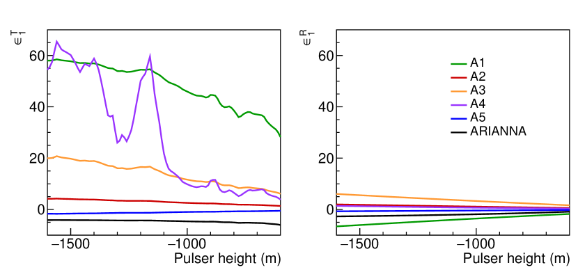
Figure 6: Angles that the electric fields make with the 12’oclock and 3 o’clock directions, called $\epsilon$ angles, for ray 1 emitted from the transmitter (left) and intersected by a receiver (right) at each station as a function of pulser height. The A1 antennas are at 80 m depth, the antennas in other ARA stations at 180 m depth, and ARIANNA antennas at the surface. For an isotropic or uniaxially birefringent medium, these epsilon angles would all vanish. The two rays have similar $\epsilon$ angles ($\lesssim 0.1^{\circ}$ difference) as can be seen in Fig. 17 in Appendix C. I note that these $\epsilon$ angles are not frequency-dependent.

There are cases where the $\epsilon$ angles vanish. As we have seen in Fig. 5, for a uniaxial crystal the symmetry necessary to maintain the eigenvectors at 12 o’clock and 3 o’clock will be maintained no matter the angle of approach. In a biaxial crystal, the symmetry about one axis that keeps the $\epsilon$ angles at zero is in general only maintained if ${\bf k}$ is in a plane formed by two of the principal axes. I note that in Jordan et al. [32], propagation was only carried out in the $\beta-\gamma$ and $\alpha-\gamma$ planes. In a biaxially birefringent medium, in the $\alpha-\gamma$ plane, there is even one angle with respect to the $\gamma$-axis where the medium appears as if it were isotropic to an incident wave (see Appendix A).

Fig. 6 shows the $\epsilon$ angles for ray 1 seen by a SPICE signal propagating from the transmitter to the receiver for the five ARA stations and ARIANNA. The differences between the $\epsilon$ angles for the two rays are small ($<0.1^{\circ}$ and are shown in Fig. 17 in Appendix C. Assuming the indicatrix is not frequency-dependent, then the epsilon angles are also not frequency-dependent. Note that the epsilon angles are often non-zero and can be large, and can change greatly between the transmitter and receiver. The non-zero epsilon angles will enable interference patterns at the receiver even in the absence of cross-polarization at the transmitter. That the epsilon angles change between the transmitter and receiver will cause a signal transmitted purely in $\theta$-pol to be detected with $\phi$-pol power. See Fig. 18 in Sec. 18 for the dependence of $\epsilon$ angles as a function of all directions of $\vec{k}$.

The $\epsilon$ angles can change between the transmitter and receiver for two reasons. First, because the indicatrix is depth-dependent, and second because the direction of ${\bf k}$ changes along the path due to the depth-dependent indices of refraction. Both of these effects change the intersection ellipse.

Which of these two effects, a depth-dependent indicatrix or a changing ${\bf k}$ along the ray, is the dominant reason for changing $\epsilon$ angles appears to be geometry-dependent. In the case of A1, the ray path is nearly a straight line as illustrated in Fig. 2, yet the $\epsilon$ angles still change significantly, and so the depth-dependence of the indicatrix must be the dominant cause of the change in that case. However, notice in Fig. 6 the dramatic changes in $\epsilon$ angles at the transmitter depths between 1500 m and 1000 m for signals destined for A4. At the same depths, we can see in Fig. 3 that the indicatrix is only changing slowly. The large changes in $\epsilon$ angles seen by signals between the transmitter and A4 must be dominated by the changing direction of ${\bf k}$. Characterizing the source-receiver geometries that will see the greatest changes in $\epsilon$ angles will be a topic of future study.

IV Experimental setup

The South Pole ice core (SPICE) was a ${\sim}40$ ka (40,000-year-old), 1500 m deep core of ice recovered in the 2014-15 and 2015-16 Austral summer seasons for investigations of glaciology and climate history from the ice at South Pole [62]. Subsequently, from Dec. 23^rd to Dec. 31^st of 2018, members of the ARA and ARIANNA collaborations lowered pulsers transmitting radio-frequency pulses into the core so that they would be observed by the (five) ARA and (one) ARIANNA stations nearby [30, 31]. This provided an unprecedented dataset for measuring signals after propagating up to 4 km horizontal distance with the transmitter and receiver both in the ice. Measurements from all six stations were made in different polarizations as a function of the depth of the pulser, from the different vantage points and distances of the six receiver stations (see diagram in Fig. 1).

The depth-dependent properties of the SPICE ice core were reported in Ref. [61] and are summarized in Fig. 3. Samples of the ice from every 20 m in the core, from 140 m to 1749 m depth, were analyzed at Penn State University using a c-axis fabric analyzer, which uses cross-polarized light to find the average orientation of the c-axis, which is the direction of approach at which the crystal behaves as an isotropic medium. As a function of depth, the c-axis was found to rotate within a vertical plane, becoming more vertical with increased depth. Although the orientation of the plane about the vertical axis is not known since the orientation of the core was not preserved during data taking, it is assumed based on understanding that it is aligned with the direction of ice flow, which is 36${}^{\circ}46^{\prime}23^{\prime\prime}$ counterclockwise from the northing direction in the northing-easting coordinate system used by South Pole surveyors.

The SPUNK PVA (SPICE Pulser from UNiversity of Kansas Pressure Vessel Antenna) transmitter was an aluminum fat dipole modeled after the ones used for the RICE experiment [63], described in detail in Ref. [30]. The $9$ cm $\times~{}90$ cm antenna was made to fit the 97 mm hole and designed so that the impedance would be 50 $\Omega$ to match the cable when immersed in the estisol-240 drilling fluid environment in the hole.

ARA and ARIANNA are both neutrino experiments aiming to detect ultra-high energy neutrinos above ${\sim}10^{17}$ eV, and stations from the different detectors, ARA deep in the ice and ARIANNA at the surface, provided views of the SPICE pulser from many vantage points with respect to the principal axes of what we are treating as a biaxial crystal from varying distances. Table 1 gives the coordinates of each station near South Pole and the angle that an observer sees the pulser in the horizontal plane relative to ice flow.

The Askaryan Radio Array (ARA) is a neutrino detector at South Pole aiming to detect impulsive radio Askaryan emission from neutrino-induced cascades in the ice [64, 18, 65, 66, 31]. ARA consists of five stations of sixteen antennas deployed up to 180 m deep in the ice. Each station includes sixteen antennas, eight “VPol” and eight “HPol” (in this paper referred to as $\theta$-pol and $\phi$-pol) with bandwidths spanning 150-800 MHz. The antennas of the former type are dipoles and the latter are ferrite-loaded quad slot antennas. The antennas in a station are arranged in approximately a 20 m$\times$20 m$\times$20 m square sitting along four vertical strings, each with two $\theta$-pol, $\phi$-pol pairs of top and bottom antennas. When a 3/8 coincidence trigger in either polarization is satisfied, signals are transmitted to the surface where waveforms from all sixteen antennas are read out in approximately 1000 ns waveforms at a sampling rate of 3.2 GHz.

ARIANNA [19, 67, 68, 69, 70] is a neutrino detector aiming to detect the same Askaryan signature from neutrino-induced cascades in the ice, with nine stations at Moore’s Bay on the Ross Ice Shelf near the coast of Antarctica. ARIANNA deploys log-periodic dipole antennas (LPDAs) at the surface, and being on the ice shelf it is sensitive to neutrino-induced radio emission reflected from the ice-water boundary below.

ARIANNA deployed an additional two stations near South Pole, and in Ref. [31] reports results from observing SPICE pulsers in what they call Station 51. Station 51 consisted of eight antennas, four of which are down-facing LPDAs arranged in a 6 m$\times$6 m square and oriented to measure two horizontal polarizations perpendicular to one another in the plane of the square, at 0.5 m below the surface. There are additionally four bicone antennas oriented vertically at the corners of the square. Thus, the station measures polarizations in three mutually perpendicular directions. The ARIANNA station is sensitive in the 80 MHz-300 MHz band and digitizes signals at 1 GHz.

Station	E (m)	N (m)	Distance (m)	Depth (m)	$\angle$ (∘)
SPICE	12911	14927.3	N/A	600-1600	N/A
A1	11812.2	15560.3	1268	80	23
A2	10814.6	13828.5	2367	180	81
A3	9814.56	15561	3160	180	42
A4	10813.7	17293.4	3161	180	4.8
A5	9862.11	12114.6	4148	180	96
ARIANNA	12543.4	15356.4	565	1	3.8

Table 1: Coordinates of the SPICE ice core hole and each station in Easting and Northing, the horizontal distance between the pulser and each station, depth of pulser/receivers, and the angle $\alpha$ that each station views the pulser in the horizontal plane relative to the direction of ice flow. The ARA station positions are from [71] and the ARIANNA station position is from [72].

V Pulsers in a Biaxially Birefringent Medium

In this section, I describe the strategy that I use to model the transmission of impulses by an antenna embedded in an anisotropic medium and their propagation in the ice.  At the transmitter, the electric field of the signal will be written as the sum of the fields from two eigenstates. Along the path, the two eigenstates will follow the same path, but accumulate different phases, and their polarizations will rotate as the eigensolutions for the electric field rotate. While propagation of waves in biaxially birefringent media is well documented, it is not typical for the transmitter itself to sit within a dense medium, far less an anisotropic medium. Therefore, there are places where I need to simply propose a way to proceed.

V.1 Assumptions

I consider two different types of antennas, one of which is traditionally called VPol and the other HPol, but for greater clarity here I call them $\theta$-type and $\phi$-type, respectively, because they measure the ${\bf\hat{\bf\theta}}$ and ${\bf\hat{\bm{\phi}}}$ components of an incident field. The physical antennas of either type sit with their orientation vertical (down a hole). Where effective heights are needed, I use simple forms of those for ARA antennas given by: ${\bf h^{\theta}_{\rm eff}}=h_{0}\sin{\theta}\,{\bf\hat{{\bm{\theta}}}}$ and ${\bf h^{\phi}_{\rm eff}}=h_{0}\sin{\theta}\,{\bf\hat{{\bm{\phi}}}}$ for $\theta$-type and $\phi$-type antennas, respectively. The effective heights will in general be frequency-dependent, but I only consider a single frequency at a time in this paper.

The electric field of the signal emitted by the transmitter is related to the transmitted power and the effective height ${\bf{h}^{T}_{\rm eff}}$ of the antenna. We express the field at the transmitter as:

$${\bf E_{T}^{\rm total}}=E_{0}\,{\bf h^{T}_{\rm eff}}(\theta,\phi)/h_{0}$$ (6)

where $\theta$ and $\phi$ are the zenith and azimuth of the direction of the ray at the transmitter, and the square of $E_{0}$ is proportional to the transmitted power.

I propose that in an anisotropic medium the $\theta$ and $\phi$ in Eq.( 6) are the angles of ${\bf S}$ (not ${\bf k}$) and that while ${\bf E}$ and ${\bf D}$ are not in the same direction, it is still the electric field that is dotted into the effective height (not ${\bf D}$). Recall that ${\bf S}$ is in the direction of energy flow and ${\bf E}$ is perpendicular to ${\bf S}$. Fig. 16 in Appendix C shows the angle between ${\bf k}$ and ${\bf S_{1}}$ and ${\bf S_{2}}$ for the SPICE pulses viewed by the stations. They differ at most by about 0.2^∘, which is approximately the angular resolutions of the detectors on the directions of received signals. After the development of a more complete model for ray tracing in biaxial birefringence, the choice of ${\bf S}$ here for the vector that defines $\theta$ and $\phi$ could be experimentally tested.

It is ${\bf k}$ that satisfies Snell’s law, and so a receiver will observe a ray if its wave vector ${\bf k}$ takes a path that intersects both the transmitter and receiver in the depth-dependent indices of refraction seen by that ray [54, 73]. The reason for it being ${\bf k}$ and not ${\bf S}$ that needs to satisfy this requirement is that the phase matching condition, which leads to Snell’s law, requires that at an interface:

$${\bf k_{\rm inc}}\cdot{\bf x}={\bf k_{\rm refl}}\cdot{\bf x}={\bf k_{\rm trans}}\cdot{\bf x}$$ (7)

where ${\bf x}$ is a vector parallel to the surface and pointing to a location on the interface surface where the wave vector is incident. The subscripts denote incident, reflected, and transmitted. I call the direction of the energy flow of the ray leaving the transmitter ${\bf S_{T}}$.

V.2 Ray Tracing

Although the treatment of Snell’s law in uniaxially birefringent media is common in the literature [55], the bending of rays in biaxially birefringent media is rarely discussed due to its complexity. In Ref. [74], the authors lay out an iterative procedure to find the ray solutions, and preliminary work on this problem for in-ice neutrino detectors was presented in Ref. [75].

In this paper, I simply take the rays to bend as they would in an isotropic medium with a depth-dependent index of refraction and leave a more complete treatment for future work. I also use the same $n(z)$ for both rays leaving the transmitter for finding the ray paths. Just as in an isotropic medium, I take the rays to follow a path in the plane of the transmitter, receiver, and the vertical axis. Although the depth-dependent index of refraction does lead to both “direct” and “refracted” solutions, the latter reaching the receiver after a downward bend, for simplicity I only consider the direct ray solutions here.

Fig. 18 in Appendix D allows us to evaluate the potential impact of using ray tracing in an isotropic medium with a simple $n(z)$ even though the fields are propagated in a biaxial birefringent medium described by $n_{\alpha}$, $n_{\beta}$, and $n_{\gamma}$. Measurements of the arrival directions of SPICE pulses in ARIANNA have been consistent with those expected from ray tracing in an isotropic medium to within about $1^{\circ}$ in both zenith and azimuth [20], and ARA reports SPICE pulse arrival directions to within a few degrees in zenith in A2 [30]. Additionally, two calibration pulsers were deployed along an IceCube string in that detector’s final season of construction at a distance of 4 km, and both A2 and A3 observed arrival directions of those pulses with a few degrees in zenith and about $1-2^{\circ}$ in azimuth [64]. From Fig. 18, a deviation of the direction of ${\bf k}$ by of order a degree will not have a qualitative effect on the behavior of the $\epsilon$ angles, and thus the rotation of the polarization vectors.

In Ref. [76], the ray solutions are found for $n(z)$ profiles with the exponential form $n(z)=1.78-0.43e^{0.0132z}$ (where $z$ is negative and in meters), but I use a modified form. This is because the eigenvalues for the index of refraction seen by any given wavefront will lie between $n_{\alpha}$ and $n_{\gamma}$. Therefore, I alter the exponential parameter in the expression from Ref. [76] so that the index of refraction is between $n_{\alpha}$ and $n_{\gamma}$ at depths where they are measured while keeping $n=1.35$ at the surface and $n=1.78$ in deep ice. I instead use the profile $n(z)=1.78-0.43e^{0.03624z}$. At $150$ m depth, this shifts the index of refraction from $n=1.721$ to 1.778.

Thus the ray tracing algorithm used here is simplistic for many reasons. First, the n(z) profiles seen by each ray should be different. Second, in a biaxially birefringent medium, a ray will not in general stay in the plane we would expect in an isotropic medium. Third, as the indicatrix changes along its path, a ray would continue to split into many rays (because the incident ray solution is not an eigenvalue of the new indicatrix at each step), but I neglect this effect. This is an area that requires much additional effort.

I use a depth-dependent attenuation of the field strength that is used by Ref. [76], which comes from Ref. [77]. Thus I apply an attenuation factor $\mathcal{A}$ to account for the attenuation of the electric field along the path of the ray from the transmitter $T$ and the receiver $R$ given by:

$$\mathcal{A}=\int_{T}^{R}{e^{-ds/\ell}ds}$$ (8)

where $\ell$ is the field attenuation length at the ice depth at position $s$ along the ray’s path.

V.3 Wave propagation

In this section, I lay out the procedure I use to propagate signals from the transmitter to the receiver. Throughout, I develop the mathematical expressions for a single frequency. Impulses would of course be a sum of contributions of different frequency components with appropriate phases.

V.3.1 Simplification: Two Rays, Same Wave Vectors

Let’s begin with an approximation that for a given transmitter-receiver pair, there is only one ${\bf k}$ at the transmitter whose path in the ice will intersect the receiver. For that single ${\bf k}$ at the transmitter, there are two eigensolutions for ${\bf E}$ at the transmitter that are perpendicular to each other, and each sees a different index of refraction. I keep these as two rays that propagate at different speeds with fields ${\bf E_{\rm 1}}$ and ${\bf E_{\rm 2}}$, but always with their wave vectors in the same direction at a given depth.

The two rays will accumulate a phase difference due to seeing different indices of refraction along their path. My simplification, however, forces both rays to take the same path. So, the phase differences that we will find only come about due to the different polarizations seeing different indices of refraction on their path, not from any differences between their path lengths. For a 1 km path length, a deviation of the path trajectory by $\sim 1^{\circ}$ would lead to a path difference of approximately 1 km $\cdot\cos{1^{\circ}}=15$ cm, which at 300 MHz is half a wavelength in deep ice for $n=1.79$, so a proper treatment of ray tracing could impact the positions of the interference peaks and nulls.

V.3.2 Propagating Signals from the Transmitter to the Receiver

The signal propagation starts with finding the two eigenvectors of the electric field at the transmitter ${\bf E_{1}^{T}}$ and ${\bf E_{2}^{T}}$ given ${\bf k}$ and the indicatrix at the transmitter depth. To find these directions, we first find the eigenvectors of the displacement vector ${\bf D_{1}^{T}}$ and ${\bf D_{2}^{T}}$ corresponding to ${\bf k}$ by finding the intersection of the planar wavefront with the indicatrix. For this, I use the procedure laid out in Ref. [78] and the depth-dependent principal axes shown in Fig. 3 from [61]. The electric fields are then found from ${\bf E_{1}^{T}}={\bm{\varepsilon}}^{-1}{\bf D_{2}^{T}}$ and ${\bf E_{2}^{T}}={\bm{\varepsilon}}^{-1}{\bf D_{2}^{T}}$.

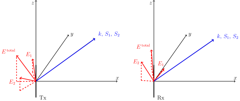
Figure 7: Vectors associated with the two rays at the transmitter (left) and the receiver (right) when the transmitter is at 1000 m depth and the receiver at station A1. The differences between the ${\bf k}$, ${\bf S_{1}}$, and ${\bf S_{2}}$ vectors are not visible in this figure; the angles between them can be found in Fig. 16 in Appendix C.

Fig. 7 illustrates the orientation of electric fields, Poynting vectors, and wave vector for the two rays leaving the transmitter and arriving at the receiver for a signal propagating from the SPICE pulser to A1. For a given ${\bf k}$ of the ray at a given depth, there are two Poynting vectors ${\bf S_{1}}$ and ${\bf S_{2}}$, one for each of the two rays. These vectors have polar angles $(\theta_{1},\phi_{1})$ and $(\theta_{2},\phi_{2})$, respectively. Although the Poynting vectors are often similar in direction (within a fraction of a degree), I keep their directions different to maintain generality.

For a given ray with Poynting vector ${\bf S_{1}}$ or ${\bf S_{2}}$, in the absence of cross-polarization power, a $\theta$-type transmitter emits an E field polarized in the ${\bf\hat{{\bm{\theta}}}^{T}_{1}}$ or ${\bf\hat{{\bm{\theta}}}^{T}_{2}}$ direction, respectively. Each ${\bf\hat{\bm{\theta}}}$ direction is perpendicular to their respective ${\bf S}$ and in the plane of ${\bf S}$ and the $\gamma$-axis since the antenna is oriented vertically.

Now we can write an expression for the total transmitted field in terms of the eigenvectors ${\bf E_{1}^{T}}$ and ${\bf E_{2}^{T}}$. In general, neither ${\bf E_{1}^{T}}$ nor ${\bf E_{2}^{T}}$ is parallel to the ${\bf\hat{\bm{\theta}}_{1}^{T}}$ or ${\bf\hat{\bm{\theta}}_{2}^{T}}$ directions respectively, but one will typically be close. I call the angle that ${\bf E_{1}^{T}}$ makes with the ${\bf\hat{\bm{\theta}}_{T}}$ direction $\epsilon_{1}^{T}$. Then ${\bf E_{2}^{T}}$ makes an angle $\epsilon_{2}^{T}$ with respect to the ${\bf\hat{\bm{\phi}}}$ direction that is typically similar to (within $\lesssim 0.2^{\circ}$ of) $\epsilon_{1}^{T}$. For generality, I maintain both variables. These are the same as the $\epsilon$ angles described in Sec. III.2. Then the transmitted purely $\theta$-pol signal is given by the sum of the $\theta$-pol components of the field from each the two rays:

$${\bm{E}^{\rm total}_{T}}= {\bm{E}_{1}^{T}}+{\bm{E}_{2}^{T}}$$ (9)

$$= E_{0}\sin{\theta_{1}^{T}}\cos{\epsilon_{1}^{T}}\,{\bf\hat{E}_{1}^{T}}$$

$$+E_{0}\sin{\theta_{2}^{T}}\sin{\epsilon_{2}^{T}}\,{\bf\hat{E}_{2}^{T}}.$$ (10)

In each term in Eq. 10, the factor containing $\theta$ is due to the transmitter beam pattern, and the factors containing $\epsilon$ pick out the component of the transmitted field that is attributed to each ray. Here we are using the beam patterns of ARA antennas expressed in Sec. V.1. For ARIANNA, the factors of $\sin{\theta}$ would be replaced with beam patterns appropriate for LPDAs, but those are not needed in this paper.

At later times, the power undergoes 1/r and attenuation losses, and I keep the fraction of power carried by each ray the same as at the transmitter, but the directions of ${\bf E_{1}}$ and ${\bf E_{2}}$ change along the rays’ path. The directions of the E fields change because the $\epsilon$ angles change with depth, as noted in Sec. III.2.

So, at an arbitrary position along the ray’s path ${\bf s}$ and time $t$:

$$r{\bf E^{\rm total}}= \mathcal{A}\left({\bf E_{1}}+{\bf E_{2}}\right)$$ (11)

$$= \mathcal{A}E_{0}\sin{\theta_{1}^{T}}\cos{\epsilon_{1}^{T}}\,{\bf\hat{E}_{1}}e^{i(\xi_{1}-\omega t)}$$

$$+\mathcal{A}E_{0}\sin{\theta_{2}^{T}}\sin{\epsilon_{2}^{T}}\,{\bf\hat{E}_{2}}e^{i(\xi_{2}-\omega t)}$$ (12)

where

$$\xi_{1,2}=\int_{T}^{R}{\bf k_{1,2}}\cdot d{\bf s}$$ (13)

and

$$r=\int_{T}^{R}d{\bf s},$$ (14)

where the limits of integration are the positions of the transmitter and receiver. Due to the assumption that the wave vectors are in the same direction at all depths, in Eq.( 12) it is the same ${\bf s}$ that appears in each term.

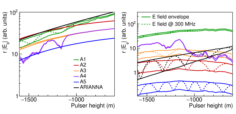
Figure 8: The electric fields expected in $\theta$-pol antennas (left) and $\phi$-pol antennas (right) with no power in cross-polarization for each station as a function of pulser height if the signal were purely at 300 MHz. In an isotropic or uniaxially birefringent medium, the signal in $\phi$-pol antennas would vanish. The solid lines show the upper and lower bounds of the envelope of the field strength, while the dashed lines show the field strengths after including the interference term at 300 MHz. The same interference term subtracts from the power in the left plot when it adds to the power in the right plot, and vice versa. The choice of frequency does not affect the envelopes, only the interference terms (dashed lines). Note the different vertical scales in the two plots.

Next, let’s consider the time-dependent voltages seen at a receiver at a distance. The (complex) voltage $\mathscr{V}$ at a $\theta$-pol receiver $R$ is given by:

$$r\mathscr{V}_{R}= {\bf E_{1}^{R}}\cdot{\bf h^{R}_{\rm eff}}(\theta_{1}^{R},\phi_{1}^{R})$$

$$+{\bf E_{2}^{R}}\cdot{\bf h^{R}_{\rm eff}}(\theta_{2}^{R},\phi_{2}^{R})$$ (15)

and using the model for effective heights described in Sec. V.1, and ${\bf\hat{\bm{\theta}}_{1}^{R}}\cdot{\bf\hat{E}^{R}_{1}}=\cos{\epsilon_{1}^{R}}$ and ${\bf\hat{\bm{\theta}}_{2}^{R}}\cdot{\bf\hat{E}^{R}_{2}}=\sin{\epsilon_{2}^{R}}$, the voltage measured at the $\theta$-type antenna becomes:

$$r\mathscr{V}_{\rm{\theta}}= \mathcal{A}E_{0}h_{0}\left[\cos{\epsilon_{1}^{T}}\cos{\epsilon_{1}^{R}}\sin{\theta_{1}^{T}}\sin{\theta_{1}^{R}}\,e^{i(\xi_{1}-\omega t)}\right.$$

$$\left.+\sin{\epsilon_{2}^{T}}\sin{\epsilon_{2}^{R}}\sin{\theta_{2}^{T}}\sin{\theta_{2}^{R}}\,e^{i(\xi_{2}-\omega t)}\right]$$ (16)

and the voltage at the $\phi$-type antenna becomes:

$$r{\mathscr{V}_{\rm{\phi}}} =\mathcal{A}h_{0}E_{0}\left[\cos{\epsilon_{1}^{T}}\sin{\epsilon_{1}^{R}}\sin{\theta_{1}^{T}}\sin{\theta_{1}^{R}}\,e^{i(\xi_{1}-\omega t)}\right.$$

$$\left.+\sin{\epsilon_{2}^{T}}\cos{\epsilon_{2}^{R}}\sin{\theta_{2}^{T}}\sin{\theta_{2}^{R}}\,e^{i(\xi_{2}-\omega t)}\right].$$ (17)

Now I consider the power at each type of antenna, using $P_{\theta}=|{\mathscr{V}_{\theta}}|^{2}$ and $P_{\phi}=|{\mathscr{V}_{\phi}}|^{2}$. If we define the following real-valued amplitudes of the different terms:

$$V_{1}^{\theta}=\mathcal{A}E_{0}h_{0}\cos{\epsilon_{1}^{T}}\cos{\epsilon_{1}^{R}}\sin{\theta_{1}^{T}}\sin{\theta_{1}^{R}}$$

$$V_{2}^{\theta}=\mathcal{A}E_{0}h_{0}\sin{\epsilon_{2}^{T}}\sin{\epsilon_{2}^{R}}\sin{\theta_{2}^{T}}\sin{\theta_{2}^{R}}$$

$$V_{1}^{\phi}=\mathcal{A}h_{0}E_{0}\cos{\epsilon_{1}^{T}}\sin{\epsilon_{1}^{R}}\sin{\theta_{1}^{T}}\sin{\theta_{1}^{R}}$$

$$V_{2}^{\phi}=\mathcal{A}h_{0}E_{0}\sin{\epsilon_{2}^{T}}\cos{\epsilon_{2}^{R}}\sin{\theta_{2}^{T}}\sin{\theta_{2}^{R}}$$ (18)

so that

$$\mathscr{V_{\theta}}=V_{1}^{\theta}e^{i(\xi_{1}-\omega t)}+V_{2}^{\theta}e^{i(\xi_{2}-\omega t)}$$ (19)

$$\mathscr{V_{\phi}}=V_{1}^{\phi}e^{i(\xi_{1}-\omega t)}+V_{2}^{\phi}e^{i(\xi_{2}-\omega t)}$$ (20)

then we can now put the power in each polarization into a simpler form:

$$r^{2}P_{\theta}= |r\mathscr{V}_{1}^{\theta}|^{2}+|r\mathscr{V}_{2}^{\theta}|^{2}$$

$$+ r^{2}V_{1}^{\theta}V_{2}^{\theta}\left[e^{i(\xi_{1}-\xi_{2})}+e^{-i(\xi_{1}-\xi_{2})}\right]$$ (21)

$$= (rV_{1}^{\theta})^{2}+(rV_{2}^{\theta})^{2}$$

$$+ 2r^{2}V_{1}^{\theta}V_{2}^{\theta}\cos{(\xi_{1}-\xi_{2})}$$ (22)

and then by adding and subtracting $2V_{1}^{\theta}V_{2}^{\theta}$, and using $\cos{y}=(e^{iy}+e^{-iy})/2$ and $\sin^{2}{y}=(1-\cos{2y})/2$, we can write:

$$r^{2}P_{\theta} =r^{2}(V^{\theta}_{1}+V^{\theta}_{2})^{2}$$

$$-4r^{2}V^{\theta}_{1}V^{\theta}_{2}\sin^{2}{\left[\dfrac{\xi_{1}-\xi_{2}}{2}\right]}.$$ (23)

Similarly for the $\phi$-type antennas,

$$r^{2}P_{\phi}= r^{2}(V^{\phi}_{1}+V^{\phi}_{2})^{2}$$ (24)

$$-4r^{2}V^{\phi}_{1}V^{\phi}_{2}\sin^{2}{\left[\dfrac{\xi_{1}-\xi_{2}}{2}\right]}.$$

In Appendix B, Fig. 14 shows the terms in Eqs. 23 and 24 evaluated for each station observing the SPICE pulses.

Fig. 8 shows the electric fields expected at the location of the $\theta$-pol and $\phi$-pol receiver antennas as a function of pulser depth for each station at 300 MHz and with no cross-polarization response in the antennas. Fig. 15 in Appendix B shows the expected voltages in ARA antennas after the antenna responses have been folded in. In the absence of a biaxial treatment of birefringence with no cross-polarization power, the $\phi$-pol antennas would not observe any signal. We can see that as a function of distance, the most the power in a $\theta$-pol antenna can be is $(V_{1}^{\theta}+V_{2}^{\theta})^{2}$ and the least it can be is $(V_{1}^{\theta}-V_{2}^{\theta})^{2}$ (and similarly for $\phi$-pol), and these bounds form an “envelope.” We can see an interference term in the second line of Eqs. 23 and 24, and the expected voltages including the interference terms are shown as dashed lines in Fig. 15.

When the $\epsilon$ angles go to zero and in the absence of cross-polarization power, to a good approximation the voltages at the receivers get to the form expected for the isotropic case. When $\epsilon_{1}^{T}=\epsilon_{2}^{T}=\epsilon_{1}^{R}=\epsilon_{2}^{R}=0$, then the voltages at the two types of receivers become:

$$r\mathscr{V}_{\theta}= \mathcal{A}E_{0}h_{0}\sin{\theta_{1}^{T}}\sin{\theta_{1}^{R}}\,e^{i(\xi_{1}-\omega t)}$$ (25)

$$r\mathscr{V}_{\phi}= 0,$$ (26)

and so there is no power in the $\phi$-type antenna when we transmit from a $\theta$-type antenna. This is the same as the expression we would find for $r\mathscr{V}_{\theta}$ for the isotropic case. Remember that because of ray bending due to depth-dependent indices of refraction, $\theta_{1}^{R}\neq\theta_{1}^{T}$. I name the following prefactor for the next section:

$$\mathcal{F}=\mathcal{A}E_{0}h_{0}\sin{\theta_{1}^{T}}\sin{\theta_{1}^{R}}.$$ (27)

V.3.3 The Power Envelope and Interference

In this section, I discuss important aspects of the formalism developed in Sec. V.3 to develop intuition. These are the power envelope and the interference terms.

While power in Eqs. 23 and  24 will oscillate as a function of distance, they will remain within an envelope whose bounds are given by $(V_{1}^{\theta}+V_{2}^{\theta})^{2}$ and $(V_{1}^{\theta}-V_{2}^{\theta})^{2}$. Approximating $\theta_{1}^{T}=\theta_{2}^{T}$, $\theta_{1}^{R}=\theta_{2}^{R}$, $\epsilon_{1}^{R}=\epsilon_{2}^{R}=\epsilon^{R}$, and $\epsilon_{1}^{T}=\epsilon_{2}^{T}=\epsilon^{T}$, the upper bound of the envelope becomes:

$$r^{2}P_{\theta}^{\rm env}= \mathcal{F}^{2}\left(\cos^{2}{\epsilon^{T}}\cos^{2}{\epsilon^{R}}+\sin^{2}{\epsilon^{T}}\sin^{2}{\epsilon^{R}}\right.$$

$$+ \left.2\cos{\epsilon^{T}}\sin{\epsilon^{T}}\cos{\epsilon^{R}}\sin{\epsilon^{R}}\right).$$ (28)

When both of the $\epsilon$ angles are zero, this becomes $r^{2}P_{\theta}^{\rm env}=\mathcal{F}^{2}$, as expected for the isotropic case.

We have seen that there is also an interference term. Using the same approximations that went into Eq. 28, this interference component of the power becomes:

$$r^{2}P_{\theta}^{\rm inter}= -4\mathcal{F}^{2}\cos{\epsilon^{T}}\cos{\epsilon^{R}}\sin{\epsilon^{T}}\sin{\epsilon^{R}}$$

$$\cdot\sin^{2}{\left(\dfrac{\xi_{1}-\xi_{2}}{2}\right)}.$$ (29)

Note that this term vanishes if one or both of the $\epsilon$ angles is zero.

The presence of the envelope and interference terms in Fig. 15 can be understood in terms of the birefringence background that I outlined in Sec. III. The variations in the envelope as a function of pulser depth originate from changes in the $\epsilon$ angles. The interference term is most important when transmitted signal power is near evenly split between the two eigensolutions.

Fig. 9 shows the time difference between the signals from the two rays arriving at the receivers for the five ARA stations and ARIANNA. Note that the two pulses will only interfere in time at a receiver if the widths of the arriving pulses are broader than the difference in arrival times between them shown in the figure.

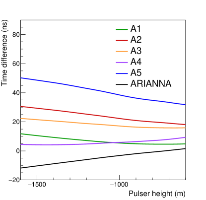
Figure 9: Time difference between the two rays (both direct rays) emitted from the SPICE transmitter at different pulser heights upon arrival at each station. For the two pulses to interfere, the width of the pulses in time would need to be longer than the time differences shown here when incident on the receivers. The curve in this plot representing time differences in A2 is consistent with what is shown in [30].

Even if the pulses do not interfere in time, then birefringence will leave an imprint in the received spectrum if both pulses are captured in the digitized waveform. The argument of the $\sin^{2}$ function is given by:

$$\dfrac{\xi_{1}-\xi_{2}}{2}=\int_{T}^{R}\left(k_{1}-k_{2}\right){\bf\hat{k}}\cdot d{\bf s},$$ (30)

where $k_{1,2}=2\pi n_{1,2}f/c$ with $n_{1,2}$ being the indices of refraction seen by the two rays, which depends on ${\bf k}$. So this becomes:

$$\dfrac{\xi_{1}-\xi_{2}}{2}=\dfrac{\pi f}{c}\int_{T}^{R}\left(n_{1}-n_{2}\right){\bf\hat{k}}\cdot d{\bf s}.$$ (31)

If we substitute:

$$c\Delta t=\int_{T}^{R}\left(n_{1}-n_{2}\right){\bf\hat{k}}\cdot d{\bf s}$$ (32)

where $\Delta t$ is the difference in arrival times of the two rays at the receiver, then this interference term has nulls when $(\xi_{1}-\xi_{2})/2=\pi f\Delta t=j\pi$ for integers $j$, or at frequencies given by:

$$f_{j}=\dfrac{j}{\Delta t}.$$ (33)

So, for a distance $d=1$ km and a typical $\Delta n=0.005$, there are nulls in the spectrum every $\Delta f=c/(\Delta n\,d)\approx 60$ MHz.

If we flip this around, when observable, the size of the increments in frequency between nulls is a measure of the distance to the source if the depth-dependent indicatrix is known. For nulls in a spectrum separated by $\Delta f$, the rays have taken a path of length given by Eq. 32. In order for the interference term to be observable, the factor $\cos{\epsilon_{1}^{T}}\cos{\epsilon_{1}^{R}}\sin{\epsilon_{1}^{T}}\sin{\epsilon_{1}^{R}}$ in Eq. 29, after accounting for cross-polarization, needs to be large enough to make the deviation from the envelope detectable.

Ref. [22] also predicts interference patterns, supported by radar data from Greenland. They report significant interference at frequencies of 30 MHz and 60 MHz for radar in 3600 m and 1200 m-thick ice for typical ice fabrics in polar ice sheets.

V.4 Cross-polarization

The SPUNK $\theta$-type antenna will also transmit some power in $\phi$-pol, and this is called cross-polarization. Ref. [30] states that from lab measurements, the power in cross-pol is reduced to 6 dB below, or 25% of, the co-polarization ($\theta$-pol) signal power. Ref. [31] reports lab measurements of cross-polarization signal from the IDL-1 pulser at 60^∘ from the maximum gain of the antenna. From Fig. 3 of that reference, the cross-polarization voltage appears to be about 20% of the co-polarization voltage, which would be about 4% in power. This fraction of the power in the cross-polarization may depend on frequency as well as the angle of transmission.

While detectable radio emission from in-ice neutrino interactions is expected to be linearly polarized with a strong vertical component, neutrino-induced emission will not be purely vertically polarized. I expect that the same formalism as the one presented here can be applied when modeling emission from neutrino interactions rather than from pulser antennas.

I simply simulate cross-polarization by rotating the polarizations of the transmitted electric field and/or the polarization of the receiver by an angle $\delta_{\rm tx}$ ( $\delta_{\rm rx}$) about the direction of ${\bf S}$ for a given ray. This is a natural way to allow for the electric field to have components in two perpendicular directions, and is the same approach as was used in Ref. [79]. The effect on $\epsilon$ angles is additive, such that:

$$\epsilon_{1}^{T}\rightarrow\epsilon_{1}^{T}+\delta_{tx},$$ (34)

similarly for $\epsilon_{2,T}$,

$$\epsilon_{1}^{R}\rightarrow\epsilon_{1}^{R}+\delta_{rx},$$ (35)

and similarly for $\epsilon_{2}^{R}$. For a cross-polarization angle of $\delta=10^{\circ}$, the fraction of power in the cross-polarization is $\left(\sin{10^{\circ}}/\cos{10^{\circ}}\right)^{2}\approx 3\%$. For $\delta=20^{\circ}$, the fraction is approximately 13%.

Cross-polarization can create an effective $\epsilon$ even where one would otherwise be zero. This leads to interference patterns observable at the receiver that would not have otherwise been present, as we will see in Section VI where I compare predictions with data.

VI Comparisons with SPICE Data

Next, I compare predictions between the model described here using published results by both the ARA and ARIANNA experiments from the SPICE pulser campaign. Note that the framework laid out here is all single-frequency, and proper comparisons with impulsive events will require an accounting of the complex signal spectrum folded in with frequency-dependent effects such as antenna responses and attenuation in the ice. The purpose here is to demonstrate that qualitatively, behaviors are observed in the data that can be brought about by signals at these frequencies propagating in ice that effectively is biaxially birefringent with principal axes used here.

I note a couple of things to keep in mind for these comparisons. Where I refer to a model for uniaxial birefringence, I have set $n_{\beta}$ to the measured $n_{\alpha}$ at a given depth, with an axis of symmetry about the ${\gamma}$-axis. Also, I include the interference term, which is valid for modeling spectra as long as signals from both rays are contained in a measured waveform. For quantities measured in the time domain such as peak voltage, the effect of the interference term will be more complicated if the pulses are only partially overlapping or not overlapping at all. As can be seen in Ref. [30], the width of the SPICE pulses observed in ARA is approximately 50 ns.

VI.1 Non-trivial rotation of polarizations

In Fig. 10, I compare the predicted ratio of voltages in the two polarizations ($V_{\phi}/V_{\theta}$) with ratios of SNRs derived from Figs. 10 and 12 in Ref. [30] for two ARA stations, A1 and A3 (although ratios of voltages and ratios of SNRs are not the same, for SNRs of about 10 as in Figs. 10 and 12, comparisons of SNRs and amplitudes are similar at the ${\sim}10$% level). We compare at four frequencies: 300 MHz, 350 MHz, 400 MHz, and 450 MHz. Ref. [30] reports measured signal SNRs in the four top and bottom $\theta$-pol and $\phi$-pol antennas, respectively. I compare with data points from the greatest pulser depths in the plot up to the shadow zone boundary at 600 m depth so that we are only comparing direct signals. Fig. 10 includes predictions for different choices of antenna cross-polarization angles, with the solid lines representing $\delta_{tx}=10^{\circ}$ and $\delta_{rx}=-10^{\circ}$. Note that these $\delta$ angles are the only free parameters in this model. We see that the model for pulses transmitted and received in ice that is effectively biaxially birefringent leads to $\phi$-pol power exceeding $\theta$-pol power, as observed in the data, at all four frequencies in A1. The reason for this is that for SPICE signals that reach A1, the epsilon angles that the signal sees at the receiver differ greatly from those that it sees at the transmitter, causing the signal polarization to rotate correspondingly.

Fig. 10 also includes uniaxial and isotropic models. In a uniaxial crystal, the $\epsilon$ angles vanish and do not change along the rays’ path, and so the power envelopes do not change, but we still expect interference between the two rays. So, the structure observed in the uniaxial models is from interference alone. In an isotropic medium, we expect that the power observed in each polarization at the receiver is the same as they were at the transmitter, which for the choice of $\delta_{tx}=-\delta_{rx}=10^{\circ}$ is $(\sin{10^{\circ}}/\cos{10^{\circ}})^{2}~{}\approx~{}3$%.

Although I do not claim that Fig. 10 shows good agreement between the model and the data at any single frequency for both stations, qualitatively it looks promising. The model does predict $V_{\phi}/V_{\theta}>1$ in A1, as is observed in the data, for some frequencies in ARA’s band for reasonable cross-polarization angles $\delta_{rx}$ and $\delta_{tx}$. In A3, $V_{\phi}/V_{\theta}$ ratios approaching unity are achieved for some frequencies as well, but for higher cross-polarization fractions corresponding to $\delta$ angles of around 20^∘. With uniaxial birefringence, this fraction does not come as close to the data points, and the data and prediction are even more discrepant for isotropic ice.

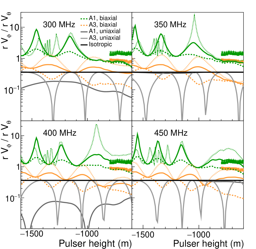
Figure 10: Ratios of signal voltages expected in $\phi$-pol and $\theta$-pol at single frequencies in stations A1 and A3 compared with measured ratios of voltage SNRs in the two polarizations (points). The lines are for antenna cross-polarization angles $\delta_{\rm rx}=-\delta_{\rm tx}=0^{\circ}$ (dashed), $10^{\circ}$ (solid), and and $20^{\circ}$ (dotted). Note that I chose solid lines for $\delta_{\rm rx}=-\delta_{\rm tx}=10^{\circ}$. The square markers are from the top pairs of $\theta$-pol, and $\phi$-pol antennas in a station, and the stars from the bottom pairs. The takeaway is that the high $rV_{\phi}/rV_{\theta}$ ratios observed from SPICE pulses in ARA stations are difficult to achieve with either uniaxial birefringence or isotropic ice, but are achievable with a biaxial treatment of birefringence at some frequencies for some choices of $\delta_{\rm rx}$ and $\delta_{\rm tx}$. The $\delta$ angles are the only free parameters in these predictions.

VI.2 Interference

In Fig. 11, I compare predictions to the polarization angle $\Psi$ reported by ARIANNA in Ref. [31] as a function of pulser depth. The polarization angle in Ref. [31] is related to the ratio of voltages in two polarizations by:

$$\Psi=\tan^{-1}{\left(|\mathscr{V}_{\phi}|/|\mathscr{V}_{\theta}|\right)}.$$ (36)

For this measurement, only the LPDA antennas measuring polarization in the horizontal plane were used [80] and the paper refers to $\mathscr{V}_{\phi}$ and $\mathscr{V}_{\theta}$ as being from the fields perpendicular to the direction of propagation. Again, the only free parameters in the model predictions in this plot are the choices of $\delta_{\rm tx}$ and $\delta_{\rm rx}$. Ref. [80] states that for pulser depths more shallow than 938 m there is expected to be interference between direct and reflected rays, so comparisons are only valid for pulser depths $>938$ m. As can be seen in the figure, the prediction is frequency-dependent, but the observations are of the size expected for cross-polarization angles $\delta_{\rm rx}$ and $\delta_{\rm tx}$ of several degrees.

Also shown is the expectation for a uniaxial ice crystal with cross-polarization included, which does not show the dramatic depth-dependent structure. The way I set the parameters of the uniaxial crystal for these comparisons gives a long distance for the oscillations, making the uniaxial curve on this plot nearly flat. For the uniaxial case with no cross-polarization, the $\Psi$ angle vanishes, also shown. Note the vertical axis goes negative to make this visible.

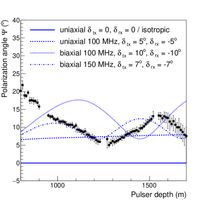
Figure 11: Comparison of measured polarization angle $\Psi$ of the SPICE pulser in the ARIANNA South Pole station with predictions at single frequencies in ARIANNA’s band and for different choices of the percentage of power in cross-polarization. I also show the case of uniaxial birefringence for $\delta_{tx}=-\delta_{rx}=5^{\circ}$ and for no cross-polarization. For pulser depths more shallow than 938 m there is expected to be interference between direct and reflected rays [80], so comparisons are only valid for pulser depths $>938$ m.

In Ref. [31] ARIANNA also shows a measured SPICE pulser spectrum that does not appear to agree in shape with the one measured in the laboratory, with dips every ${\sim}75$ MHz (see their Fig. 7). Recall that dips in the spectrum are predicted in increments of $\Delta f=1/\Delta t$. From the time differences in Fig. 9, at the greatest pulser depths I would expect oscillations in the spectrum every ${\sim}1/(\Delta t)=1/12$ ns=83 MHz. While this is suggestive, a more complete model of the station so near the surface may be needed to compare the measured spectrum with an expectation derived from the model in this paper.

In Fig. 12, I compare the predicted voltages in $\theta$-pol antennas in A5 with those reported in Fig. 13 of Ref. [30].

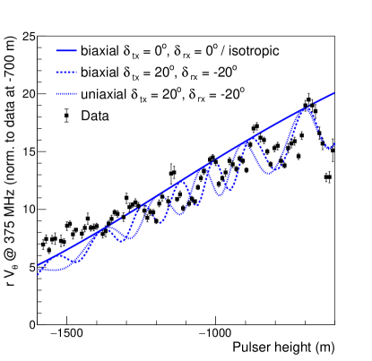
Figure 12: Peak voltage measured in $\theta$-pol antennas at the A5 station as a function of SPICE pulser height, compared to predictions at 300 MHz for different choices of cross-polarization power fraction. The models are scaled to the measurement at 700 m pulser depth.

The model shows oscillations of the magnitude seen in the data whether the model uses a uniaxially or biaxially birefringent crystal and for cross-polarization angles of about $\delta_{\rm tx}=-\delta_{\rm rx}=20^{\circ}$. These oscillations are due to interference between the rays at the receiver and rely on the pulses from the two rays overlapping in time on arrival at the receiver. Due to the small $\epsilon$ angles for station A5 seen in Fig. 6, variations in the signal envelope are small, and variations are dominated instead by interference. In this case, the interference is present whether the crystal is modeled as uniaxially or biaxially birefringent.

Additionally, I note that in Ref. [34], similar periodic variations in the power spectrum every ${\sim}200$ MHz are also reported in signals that were transmitted from the surface of the Ross Ice Shelf and received after reflections from the ice-sea water interface below. They also report observing power in the cross-polarization that is frequency-dependent and peaks at 80% of the total received power at 450 MHz, and that was only seen in in-ice measurements and not those taken in air. The authors do suggest that the modulation could be due to birefringence, with two signals arriving at different times due to wave speeds that differ by 0.1%. For the measurements reported in Ref. [34], signals were transmitted vertically, and under a model where the vertical axis is a principal axis of the indicatrix, there would still be two extraordinary rays that could interfere and cause the structure in the spectrum in the co-polarization. However, the $\epsilon$ angles would vanish, and so under that model, power in the cross-polarization would not appear beyond what was transmitted. Still, Ref. [22] notes that on ice shelves, in deep ice, and ice caps near the coast, the crystal fabric can have a more complicated structure due to being warmer and strains being more complex. Ref. [34] recommended that future measurements be taken at many angles with respect to the ice fabric.

Lastly, I note that in Ref. [18], ARA reported calibration pulses nominally transmitted in $\theta$-pol and observed after propagating approximately 3.2 km in the ice with a significant $\phi$-pol component, about a factor of 2-3 weaker in amplitude. The higher-than-expected $\phi$-pol power was attributed to radiation of cross-polarization power at the transmitter due to challenges in antenna construction during rapid deployment. Birefringence could be investigated as contributing to the observed $\phi$-pol power.

In summary, the model presented in this paper can bring about expected behaviors that are difficult to explain without a biaxial treatment of birefringence. However, we have seen that the same model parameters do not give a best fit to all of the data at once. For example, Fig. 10 and Fig. 11 seem to prefer cross-polarization angles $\delta_{rx}$ and $\delta_{rx}$ of approximately $10^{\circ}$, while Fig. 12 seems to indicate a need for higher cross-polarization angles. This could be due to one or more aspects of the model being incomplete. In addition to the aforementioned need for a broadband treatment, the indicatrix may be oversimplified, as is surely the method used to model cross-polarization.

VII Future Work

Further work is needed for more quantitative comparisons with the broadband signals in the SPICE dataset. For example, true antenna beam patterns of all types as well as the true complex pulse spectrum should be included in the model. A ray-tracing algorithm for propagating both direct and refracted signals in biaxially birefringent ice is also needed. Ideally, a finite-difference time-domain simulation could be used to validate a more complete model, although it would need to be tested over shorter distances (100s of meters) for manageable computational times [27]. In addition, the model needs to be made more general to loosen the assumption that two axes of the indicatrix are perfectly aligned with the vertical direction and along the direction of ice flow, since measurements from the ice report that they could be different by approximately 10^∘ [22].

VIII Conclusions

Data from the SPICE pulser program strongly suggest that a biaxial treatment of birefringence in the ice near South Pole, with principal axes defined by the directions of ice flow and vertical compression, has an important effect on the power of signals observed by antennas in the ice measuring different polarizations. Observed power in the two polarizations has a non-trivial dependence on the positions of the transmitter and receiver and the orientation of the pair relative to the principal axes of the birefringent crystal. While deviations compared to the isotropic or uniaxial expectations would be present even if the transmitter were to emit purely in one polarization, they are enhanced when there is some cross-polarization power transmitted and received.

While the effects described here add complexity to neutrino detection using radio techniques in in-ice detectors, the same effects provide important signatures for the identification of signals originating from neutrinos in the ice. For example, the arrival of two rays with the expected time differences of order tens of ns from nearly the same direction will be an important signature of an in-ice interaction. Then, the distance to the source can be traced using the difference in time arrival between the two rays (evident in either the time or frequency domains). This will broaden the category of events whose distance can be reconstructed more precisely than those relying on wavefront curvature, alongside the “double-pulse” events that contain both direct and refracted pulses. The distance to the interaction is crucial for reconstructing the energy of the neutrino-induced shower. Birefringence that is effectively biaxial at radio frequencies also needs to be handled properly to reconstruct the polarization of the signal at the interaction, which is required for reconstructing the direction of the incident neutrino source.

Neutrino directional reconstruction will require some knowledge of the birefringence parameters along the signal’s path. These parameters could be derived in advance from in-ice pulser data like SPICE (for in-ice experiments), or from radar data such as that from CReSIS [81]. Refs. [38, 39, 40, 41, 42, 43, 44, 45] have demonstrated that radar polarimetry can be used to extract properties of the COF as well as from measurements taken through the more laborious extracting of ice cores. Seismology measurements have also been used to extract properties of the COF [82, 42, 83]. Alternatively, perhaps enough information about the crystal could be extracted from the neutrino signal itself to enable its reconstruction.

The effects described here will also impact the design of detectors. Some care will need to be taken to optimize an array for the greatest science potential, which may be a balance between the desire to detect high power in one polarization (for example, in-ice detectors can more easily measure $\theta$-pol) and the desire to observe signatures that are more visible in the other polarization (for example, oscillations are more apparent in $\phi$-pol). The most optimal arrangement of antennas in an in-ice array may or may not have a symmetry around the direction of ice flow. For example, since changing polarizations due to rotating eigenstates is maximal in the $\alpha$-$\gamma$ plane, detectors could be designed to view away from that plane to avoid such large variations. On the other hand, if such variations could be exploited to improve reconstruction, then detection of interactions from the $\alpha$-$\gamma$ plane would be desirable. Similarly, the importance of viewing the time differences between the two rays, which at South Pole are maximal for directions along the $\beta$-$\gamma$ plane and can be used for distance reconstruction, should also be considered. While the $\phi$-pol antennas deployed by ARA are adequate to have observed the effects here, in future arrays the sensitivity to the $\phi$-pol component of the signal should not be diminished without careful consideration.

IX Acknowledgements

Thank you to the SPICE team as well as the members of the ARA and ARIANNA collaborations for their contributions in producing the SPICE pulser data set, which is an excellent one for exploring these effects. I am grateful to Dave Besson for many helpful discussions on this topic and his review of the draft, and Steven Prohira for useful feedback as my thinking has evolved on how to model these effects and for important feedback on improving the clarity of the paper. Thanks to Jorge Torres for his work on polarization reconstructions that led me to think about these behaviors in the data. Thank you to S. Bektas for promptly responding with the word document of his paper for finding the ellipsoid intersection. Thank you to Justin Flaherty for helping me with some of the fundamentals of birefringence, and for feedback on the paper draft. Thank you as well to John Beacom, Dima Chirkin, William Luszczak, Chris Hirata, Roland Kawakami, and Martin Rongen for reviewing the draft and providing valuable feedback. Thanks to James Beatty, Nicholas Harty, Dave Seckel, Ilya Kravchenko, Patrick Allison, Peter Gorham, and other members of the ARA and PUEO Collaborations as well for discussions and feedback. Thanks additionally to Kenneth Jezek, Prasad Gogineni, and Carlos Martin Garcia. Any inaccuracies or errors are my own. This work was supported by National Science Foundation award 1806923.

Appendix A Special directions in South Pole ice

In a biaxially birefringent crystal, there are only two special directions of ${\bf k}$ where waves behave the same as in an isotropic medium, with only a single ray with one index of refraction, ${\bf S}\parallel{\bf k}$, and ${\bf E}\parallel{\bf D}$. These two special directions of ${\bf k}$ sit in the $\alpha-\gamma$ plane and are the two directions for which the intersection of the planar wavefront with the indicatrix becomes a circle. These two special directions make an angle $V_{z}$ with respect to the $\gamma$-axis given by [56]:

$$\cos{2V_{z}}=\dfrac{(n_{\gamma}-n_{\beta})-(n_{\beta}-n_{\alpha})}{(n_{\gamma}-n_{\alpha})}.$$ (37)

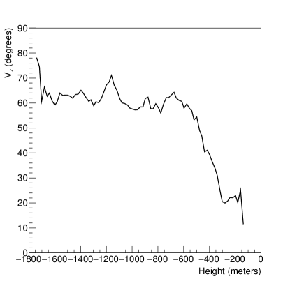
Figure 13: Treating the ice as effectively a biaxially birefringent medium at radio frequencies, there are two special directions where rays propagate as they would in an isotropic medium. These directions are in the plane of the ray and the 3-axis, each making an angle $2V_{z}$ with the 3-axis. The angle $V_{z}$ is shown here as a function of height in South Pole ice.

Fig. 13 shows the $V_{z}$ angle as a function of depth in the ice using the indicatrix parameters shown in Fig. 3. I include this plot as an interesting piece of information about South Pole ice.

Appendix B Power and voltages

In Fig. 14, I include the terms contributing to the power in $\theta$-pol (top eight plots) and $\phi$-pol (bottom eight) in Eqs. 23 and 24 for each ARA station. This plot was made at 300 MHz frequency with $\delta_{\rm tx}=\delta_{\rm rx}=0$. For $\theta$-pol, solid gray lines represent the total power and dashed gray lines represent the same but with antenna responses removed. The analogous quantities exist in $\phi$-pol as well but are not shown.

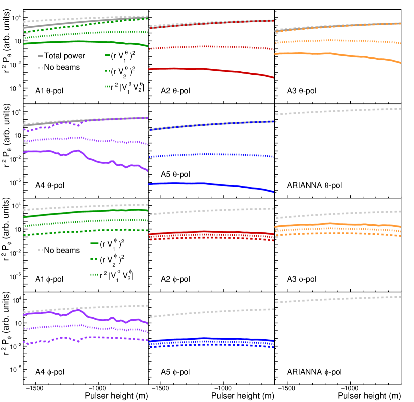
Figure 14: These figures show the terms contributing to the power at each station predicted to be measured in $\theta$-pol (top eight panels) and $\phi$-pol antennas (bottom eight). These were made at 300 MHz with no cross-polarization power in the antennas, just as in Fig. 15.

Fig. 15 shows the voltages expected in the ARA receivers calculated from the electric fields in Fig. 8 and folding in the antenna responses in Eq. 6.

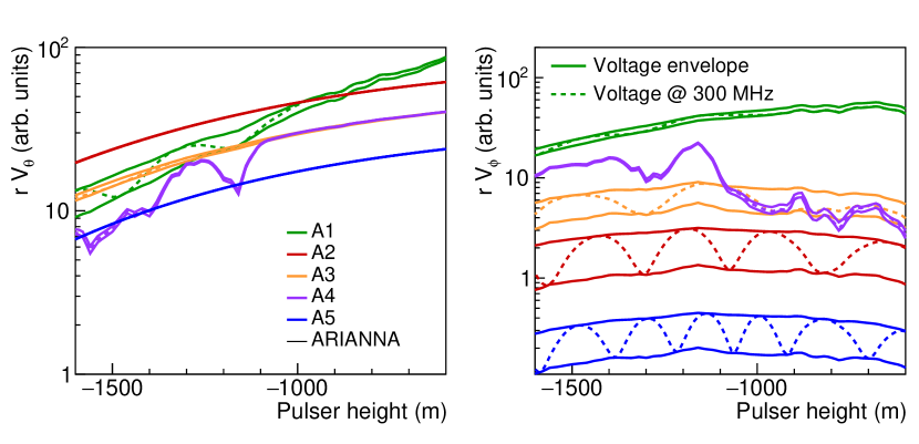
Figure 15: The voltage amplitudes expected in $\theta$-pol antennas (left) and $\phi$-pol antennas (right) with no power in cross-polarization for each station as a function of pulser height if the signal were purely at 300 MHz. In an isotropic or uniaxially birefringent medium, the signal in $\phi$-pol antennas would vanish. On the left, the lines show the upper bounds of the voltage envelope. On the right, the solid lines show the upper and lower bounds of the voltage envelope, while the dashed lines show the voltages after including the interference term at 300 MHz. The same interference term subtracts from the power in the left plot when it adds to the power in the right plot, and vice versa. Note the different vertical scales in the two plots.

Appendix C Comparing quantities in the two eigensolutions

In this section, I compare similar quantities in the two different eigenstates for a given $\vec{k}$ at a given depth relevant to the SPICE pulser data. In this paper, both rays representing the two eigensolutions are given the same ${\bf k}$ at each depth, but the direction of the corresponding Poynting vectors ${\bf S_{1}}$ and ${\bf S_{2}}$ differ slightly, as do the orientation of the electric fields about the Poynting vectors, $\epsilon_{1}$ and $\epsilon_{2}$.

Fig. 16 shows the angles between ${\bf k}$ and each of ${\bf S_{1}}$ and ${\bf S_{2}}$ at the transmitter as a function of pulser height. We can see that this angle is sub-degree for all pulser depths. In this paper, I take the angles relevant to the antenna responses to be in the direction of the Poynting vectors rather than ${\bf k}$, and the direction of the propagation of the rays to be in the ${\bf k}$ direction, not ${\bf S}$. This figure shows that these choices will have a negligible impact on the results in this paper and although would be interesting to validate in the future with data, would be challenging given angular resolutions of experiments.

Fig. 17 shows the difference between epsilon angles for the two eigenstates at the transmitter and receiver. These angles are also similar to one another to within less than about $0.1^{\circ}$.

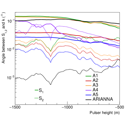
Figure 16: Angle between the wave vector $\vec{k}$ and the Poynting vectors $\vec{S}_{1,2}$ for the two corresponding eigenstates at the transmitter, as a function of depth of the pulser.

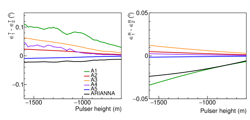
Figure 17: Angle between the $\epsilon$ angles for the two eigensolutions at the transmitter (left) and receiver (right).

Appendix D Dependence of $\epsilon$ angles on direction of ${\bf k}$

Fig. 18 shows the epsilon angle $\epsilon_{1}$ as a function of the direction of the ${\bf k}$ expressed in zenith and azimuthal angles, for 200 m and 1700 m depths. The contours are lines of equal $\epsilon$. The vertical and horizontal lines are directions where ${\bf k}$ is in a plane containing the $\alpha-\beta$, $\beta-\gamma$, or $\alpha-\gamma$ axes. We can see that in those planes the $\epsilon$ angles go to zero, but in the $\alpha$-$\gamma$ plane, the $\epsilon$ angles can change rapidly in directions deviating from that plane.

In the $\alpha$-$\gamma$ plane, there is a direction of ${\bf k}$ where the directions of the eigenvectors become indeterminant and the contours converge. This corresponds to the direction in which the intersection of the planar wavefront with the indicatrix becomes a circle, and so the axes of the intersection ellipse that normally define the directions of the eigenvectors are undefined. This is the same as the $V_{z}$ angle in Fig. 13. For example, at 200 m depth, the contours converge at $\theta\approx 20^{\circ}$ in the $\alpha$-$\gamma$ plane, and at 1700 m depth at $\theta\approx 70^{\circ}$, which are the values of $V$ at those depths in Fig. 13.

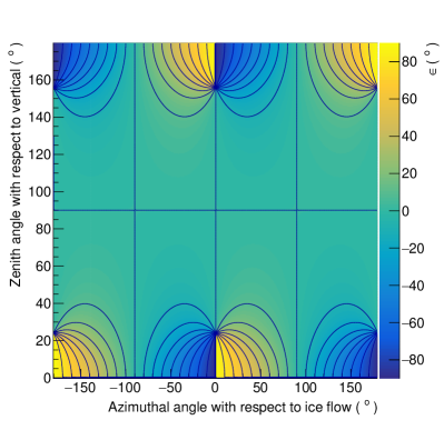
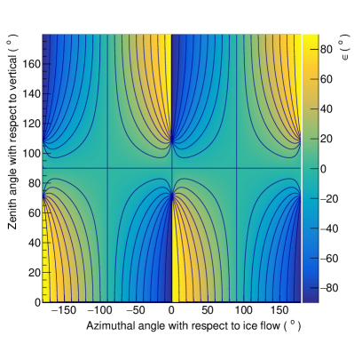
Figure 18: Angle $\epsilon_{1}$ as a function of direction of ${\bf k}$ at 200 m depth (left) and 1700 m depth (right). Following Fig. 3, at 200 m depth, $n_{\alpha}=1.77850$, $n_{\beta}=1.77900$, and $n_{\gamma}=1.78150$ are used for this figure, and at 1700 m, $n_{\alpha}=1.77700$, $n_{\beta}=1.78125$, and $n_{\gamma}=1.78175$ are used. The vertical and horizontal lines correspond to directions that lie in the $\alpha-\beta$, $\beta-\gamma$, or the $\alpha-\gamma$ plane. The points where the contours meet correspond to the lines in the $\alpha$-$\gamma$ plane where the intersection ellipse becomes a circle and the directions of the eigenvectors are undefined. These occur at zenith angles equal to the $V_{z}$ angle in Fig. 13. At 200 m depth, $V_{z}$ is about 20^∘ and at 1700 m depth it is approximately 65^∘, corresponding to the zenith angle of the points where the contours converge in the left the right plots, respectively.

Appendix E Orientation of the principal axes

Many past investigations related to radio-frequency birefringence in polar ice sheets, including previous studies interpreting SPICE pulser data in the context of birefringence in South Pole ice mentioned in Sec. I, have assumed that the indicatrix is oriented with the $\gamma$-axis vertical and another principal axis in the direction of ice flow. However, measurements in other locations have found that these assumptions do not hold at the $\sim 10^{\circ}$ level, which is likely also true at South Pole.

The “tilt” angle that the $\gamma$-axis makes with the vertical direction can be obtained from either measurements of ice cores or radar measurements. Matsuoka et al. [22] summarizes results of core measurements where the tilt angle is several degrees at many sites in both Greenland and Antarctica. J. Li et al. [46] used multi-polarization radar measurements at the NEEM site to ascertain a tilt angle of 9.6^∘ from the vertical axis.

Typically when ice cores are extracted, the azimuthal angle of the core is not preserved. Radar measurements do have the ability to extract this orientation. For example, Jordan et al. [32] found the direction of the $\beta$- axis at the North Greenland Eemian Ice Drilling (NEEM) ice core region in Greenland to be as much as 25^∘ away from its nominally expected direction perpendicular to flow, and that it changed by about 10^∘ between sites separated by a few km. T.J. Young et al. [38] estimated the ${\alpha}$-axis to be 14^∘ from the direction of ice flow at WAIS Divide in Antarctica.

As can be seen from Fig. 18, uncertainties on the orientation of principal axes of order several degrees at South Pole would, from some ${\bf k}$ directions, impact the $\epsilon$ angles and thus the polarization directions by of order 10^o, and this would directly impact the ability to reconstruct the direction of a neutrino. In Ref. [43], it was shown (see Fig. 10) that tilt angles of about 10^∘ can lead to 20% uncertainties on the difference between $n_{\alpha}$ and $n_{\beta}$, which affects delay times and thus distance and energy reconstruction. Uncertainties in the orientation relative to ice flow would have a similar effect.

References

- Aartsen et al. [2018a] M. G. Aartsen et al. (Liverpool Telescope, MAGIC, H.E.S.S., AGILE, Kiso, VLA/17B-403, INTEGRAL, Kapteyn, Subaru, HAWC, Fermi-LAT, ASAS-SN, VERITAS, Kanata, IceCube, Swift NuSTAR), Multimessenger observations of a flaring blazar coincident with high-energy neutrino IceCube-170922A, Science 361, eaat1378 (2018a), arXiv:1807.08816 [astro-ph.HE] .
- Aartsen et al. [2018b] M. G. Aartsen et al. (IceCube), Neutrino emission from the direction of the blazar TXS 0506+056 prior to the IceCube-170922A alert, Science 361, 147 (2018b), arXiv:1807.08794 [astro-ph.HE] .
- Abbott et al. [2017a] B. P. Abbott et al. (LIGO Scientific, Virgo, Fermi-GBM, INTEGRAL), Gravitational Waves and Gamma-rays from a Binary Neutron Star Merger: GW170817 and GRB 170817A, Astrophys. J. 848, L13 (2017a), arXiv:1710.05834 [astro-ph.HE] .
- Aartsen et al. [2013a] M. G. Aartsen et al. (IceCube), Evidence for High-Energy Extraterrestrial Neutrinos at the IceCube Detector, Science 342, 1242856 (2013a), arXiv:1311.5238 [astro-ph.HE] .
- Aartsen et al. [2015] M. G. Aartsen et al. (IceCube), Evidence for Astrophysical Muon Neutrinos from the Northern Sky with IceCube, Phys. Rev. Lett. 115, 081102 (2015), arXiv:1507.04005 [astro-ph.HE] .
- Aartsen et al. [2013b] M. G. Aartsen et al. (IceCube), First observation of PeV-energy neutrinos with IceCube, Phys. Rev. Lett. 111, 021103 (2013b), arXiv:1304.5356 [astro-ph.HE] .
- Abbott et al. [2016] B. P. Abbott et al. (Virgo, LIGO Scientific), Observation of Gravitational Waves from a Binary Black Hole Merger, Phys. Rev. Lett. 116, 061102 (2016), arXiv:1602.03837 [gr-qc] .
- Abbott et al. [2017b] B. P. Abbott et al. (LIGO Scientific, Virgo), GW170817: Observation of Gravitational Waves from a Binary Neutron Star Inspiral, Phys. Rev. Lett. 119, 161101 (2017b), arXiv:1710.05832 [gr-qc] .
- Ackermann et al. [2019a] M. Ackermann et al., Astrophysics Uniquely Enabled by Observations of High-Energy Cosmic Neutrinos, Bull. Am. Astron. Soc. 51, 185 (2019a), arXiv:1903.04334 [astro-ph.HE] .
- Ackermann et al. [2019b] M. Ackermann et al., Fundamental Physics with High-Energy Cosmic Neutrinos, Bull. Am. Astron. Soc. 51, 215 (2019b), arXiv:1903.04333 [astro-ph.HE] .
- Aartsen et al. [2017a] M. G. Aartsen et al. (IceCube), Measurement of the multi-TeV neutrino cross section with IceCube using Earth absorption, Nature 551, 596 (2017a), arXiv:1711.08119 [hep-ex] .
- Bustamante and Connolly [2019] M. Bustamante and A. Connolly, Extracting the Energy-Dependent Neutrino-Nucleon Cross Section above 10 TeV Using IceCube Showers, Phys. Rev. Lett. 122, 041101 (2019), arXiv:1711.11043 [astro-ph.HE] .
- Aartsen et al. [2017b] M. G. Aartsen et al. (IceCube), The IceCube Neutrino Observatory: Instrumentation and Online Systems, JINST 12 (03), P03012, arXiv:1612.05093 [astro-ph.IM] .
- Aartsen et al. [2021] M. G. Aartsen et al. (IceCube-Gen2), IceCube-Gen2: the window to the extreme universe, J. Phys. G 48, 060501 (2021), arXiv:2008.04323 [astro-ph.HE] .
- Prohira et al. [2021a] S. Prohira et al. (Radar Echo Telescope), The Radar Echo Telescope for Cosmic Rays: Pathfinder experiment for a next-generation neutrino observatory, Phys. Rev. D 104, 102006 (2021a), arXiv:2104.00459 [astro-ph.IM] .
- Abarr et al. [2021] Q. Abarr et al. (PUEO), The Payload for Ultrahigh Energy Observations (PUEO): a white paper, JINST 16 (08), P08035, arXiv:2010.02892 [astro-ph.IM] .
- Gorham et al. [2009] P. W. Gorham et al. (ANITA), The Antarctic Impulsive Transient Antenna ultra-high energy neutrino detector design, performance, and sensitivity for 2006-2007 balloon flight, Astropart. Phys. 32, 10 (2009), arXiv:0812.1920 [astro-ph] .
- Allison et al. [2012] P. Allison et al., Design and Initial Performance of the Askaryan Radio Array Prototype EeV Neutrino Detector at the South Pole, Astropart. Phys. 35, 457 (2012), arXiv:1105.2854 [astro-ph.IM] .
- Barwick et al. [2015a] S. W. Barwick et al., Design and performance of the ARIANNA HRA-3 neutrino detector systems, IEEE Transactions on Nuclear Science 62, 2202 (2015a).
- Anker et al. [2020a] A. Anker et al., White Paper: ARIANNA-200 high energy neutrino telescope, (2020a), arXiv:2004.09841 [astro-ph.IM] .
- Aguilar et al. [2021] J. A. Aguilar et al. (RNO-G), Design and Sensitivity of the Radio Neutrino Observatory in Greenland (RNO-G), JINST 16 (03), P03025, arXiv:2010.12279 [astro-ph.IM] .
- Matsuoka et al. [2009] K. Matsuoka, L. Wilen, S. P. Hurley, and C. F. Raymond, Effects of birefringence within ice sheets on obliquely propagating radio waves, IEEE Trans. Geosci. Remote. Sens. 47, 1429 (2009).
- Kravchenko et al. [2004] I. Kravchenko, D. Besson, and J. Meyers, In situ index-of-refraction measurements of the south polar firn with the rice detector, Journal of Glaciology 50, 522 (2004).
- Barwick et al. [2005] S. Barwick, D. Besson, P. Gorham, and D. Saltzberg, South Polar in situ radio-frequency ice attenuation, J. Glaciol. 51, 231 (2005).
- Avva et al. [2015] J. Avva, J. M. Kovac, C. Miki, D. Saltzberg, and A. G. Vieregg, An in situ measurement of the radio-frequency attenuation in ice at Summit Station, Greenland, J. Glaciol. 61, 1005 (2015), arXiv:1409.5413 [astro-ph.IM] .
- Deaconu et al. [2018] C. Deaconu, A. G. Vieregg, S. A. Wissel, J. Bowen, S. Chipman, A. Gupta, C. Miki, R. J. Nichol, and D. Saltzberg, Measurements and Modeling of Near-Surface Radio Propagation in Glacial Ice and Implications for Neutrino Experiments, Phys. Rev. D98, 043010 (2018), arXiv:1805.12576 [astro-ph.IM] .
- Prohira et al. [2021b] S. Prohira et al. (Radar Echo Telescope), Modeling in-ice radio propagation with parabolic equation methods, Phys. Rev. D 103, 103007 (2021b), arXiv:2011.05997 [astro-ph.IM] .
- Barwick et al. [2018] S. W. Barwick et al., Observation of classically ‘forbidden’ electromagnetic wave propagation and implications for neutrino detection, JCAP 1807 (07), 055, arXiv:1804.10430 [astro-ph.IM] .
- Besson et al. [2011] D. Besson, I. Kravchenko, A. Ramos, and J. Remmers, Radio Frequency Birefringence in South Polar Ice and Implications for Neutrino Reconstruction, Astropart. Phys. 34, 755 (2011), arXiv:1005.4589 [astro-ph.IM] .
- Allison et al. [2020a] P. Allison et al., Long-baseline horizontal radio-frequency transmission through polar ice, JCAP 12, 009, arXiv:1908.10689 [astro-ph.IM] .
- Anker et al. [2020b] A. Anker et al. (ARIANNA), Probing the angular and polarization reconstruction of the ARIANNA detector at the South Pole, JINST 15 (09), P09039, arXiv:2006.03027 [astro-ph.IM] .
- Jordan et al. [2020a] T. M. Jordan, D. Z. Besson, I. Kravchenko, U. Latif, B. Madison, A. Novikov, and A. Shultz, Modelling ice birefringence and oblique radio wave propagation for neutrino detection at the South Pole, Annals Glaciol. 61, 84 (2020a), arXiv:1910.01471 [astro-ph.IM] .
- Besson et al. [2021] D. Besson, I. Kravchenko, and K. Nivedita, Angular Dependence of Vertically Propagating Radio-Frequency Signals in South Polar Ice, (2021), arXiv:2110.13353 [astro-ph.IM] .
- Barrella et al. [2011] T. Barrella, S. Barwick, and D. Saltzberg, Ross Ice Shelf in situ radio-frequency ice attenuation, J. Glaciol. 57, 61 (2011), arXiv:1011.0477 [astro-ph.IM] .
- Chirkin and Rongen [2020] D. Chirkin and M. Rongen (IceCube), Light diffusion in birefringent polycrystals and the IceCube ice anisotropy, PoS ICRC2019, 854 (2020), arXiv:1908.07608 [astro-ph.HE] .
- Rongen et al. [2020] M. Rongen, R. C. Bay, and S. Blot, Observation of an optical anisotropy in the deep glacial ice at the geographic south pole using a laser dust logger, The Cryosphere 14, 2537 (2020).
- Matsuoka et al. [2003] K. Matsuoka, T. Furukawa, S. Fujita, H. Maeno, S. Uratsuka, R. Naruse, and O. Watanabe, Crystal orientation fabrics within the antarctic ice sheet revealed by a multipolarization plane and dual-frequency radar survey, Journal of Geophysical Research: Solid Earth 108 (2003).
- Young et al. [2021a] T. J. Young, C. Martín, P. Christoffersen, D. M. Schroeder, S. M. Tulaczyk, and E. J. Dawson, Rapid and accurate polarimetric radar measurements of ice crystal fabric orientation at the western antarctic ice sheet (WAIS) divide ice core site, The Cryosphere 15, 4117 (2021a).
- Fujita et al. [2006] S. Fujita, H. Maeno, and K. Matsuoka, Radio-wave depolarization and scattering within ice sheets: a matrix-based model to link radar and ice-core measurements and its application, Journal of Glaciology 52, 407–424 (2006).
- Matsuoka et al. [2012] K. Matsuoka, D. Power, S. Fujita, and C. F. Raymond, Rapid development of anisotropic ice-crystal-alignment fabrics inferred from englacial radar polarimetry, central West Antarctica, Journal of Geophysical Research: Earth Surface 117 (2012).
- Young et al. [2021b] T. J. Young, D. M. Schroeder, T. M. Jordan, P. Christoffersen, S. M. Tulaczyk, R. Culberg, and N. L. Bienert, Inferring ice fabric from birefringence loss in airborne radargrams: Application to the eastern shear margin of Thwaites Glacier, West Antarctica, Journal of Geophysical Research: Earth Surface 126, e2020JF006023 (2021b).
- Brisbourne et al. [2019] A. M. Brisbourne, C. Martín, A. M. Smith, A. F. Baird, J. M. Kendall, and J. Kingslake, Constraining recent ice flow history at Korff Ice Rise, West Antarctica, using radar and seismic measurements of ice fabric, Journal of Geophysical Research: Earth Surface 124, 175 (2019).
- Jordan et al. [2019] T. M. Jordan, D. M. Schroeder, D. Castelletti, J. Li, and J. Dall, A polarimetric coherence method to determine ice crystal orientation fabric from radar sounding: Application to the neem ice core region, IEEE Transactions on Geoscience and Remote Sensing 57, 8641 (2019).
- Dall [2010] J. Dall, Ice sheet anisotropy measured with polarimetric ice sounding radar, in 2010 IEEE International Geoscience and Remote Sensing Symposium (2010) pp. 2507–2510.
- Jordan et al. [2020b] T. M. Jordan, D. M. Schroeder, C. W. Elsworth, and M. R. Siegfried, Estimation of ice fabric within Whillans Ice Stream using polarimetric phase-sensitive radar sounding, Annals of Glaciology 61, 74–83 (2020b).
- Li et al. [2018] J. Li, J. A. Vélez González, C. Leuschen, A. Harish, P. Gogineni, M. Montagnat, I. Weikusat, F. Rodriguez-Morales, and J. Paden, Multi-channel and multi-polarization radar measurements around the neem site, The Cryosphere 12, 2689 (2018).
- Yan et al. [2020] J.-B. Yan, L. Li, J. A. Nunn, D. Dahl-Jensen, C. O’Neill, R. A. Taylor, C. D. Simpson, S. Wattal, D. Steinhage, P. Gogineni, H. Miller, and O. Eisen, Multiangle, frequency, and polarization radar measurement of ice sheets, IEEE Journal of Selected Topics in Applied Earth Observations and Remote Sensing 13, 2070 (2020).
- Matsuoka et al. [2004] K. Matsuoka, S. Uratsuka, S. Fujita, and F. Nishio, Ice-flow-induced scattering zone within the antarctic ice sheet revealed by high-frequency airborne radar, Journal of Glaciology 50, 382 (2004).
- Hargreaves [1978] N. D. Hargreaves, The radio-frequency birefringence of polar ice, Journal of Glaciology 21, 301 (1978).
- Fitzpatrick et al. [2021] J. Fitzpatrick, D. Voigt, J. Fegyeresi, and R. Alley, Physical properties of the south pole ice core, SPC14 (2021), IceCube Polar Science Workshop.
- Petrenko and Whitworth [2002] V. F. Petrenko and R. W. Whitworth, Physics of Ice (Oxford University Press, 2002).
- Berry and Jeffrey [2007] M. Berry and M. Jeffrey, Conical diffraction: Hamilton’s diabolical point at the heart of crystal optics, in Progress in Optics, Vol. 50, edited by E. Wolf (Elsevier, 2007) pp. 13–50.
- [53] D. Sjoberg, Electromagnetic wave propagation lecture 8: Propagation in birefringent media, https://www.eit.lth.se/fileadmin/eit/courses/eten05/ht2016/lectures/lecture8.pdf.
- Keller [2008] C. Keller, International summer school on solar polarization, Lecture 3: Crystal optics, https://home.strw.leidenuniv.nl/~keller/Teaching/China_2008/CUK_L03_handout.pdf (July 12-24, 2008).
- Orfanidis [2013] S. Orfanidis, Electromagnetic Waves and Antennas (2013) http://eceweb1.rutgers.edu/~orfanidi/ewa.
- Stoiber and Morse [1949] R. Stoiber and S. Morse, Crystal Identification with a Polarizing Microscope (Chapman & Hall, 1949).
- Nelson [2014] S. Nelson, Mineralogy, Biaxial Minerals, Tulane University EENS 2110, https://www.tulane.edu/~sanelson/eens211/biaxial.htm (2014).
- Druschel [2011] G. Druschel, University of Vermont, GEOL 110 - Earth Materials, Lecture 9: Optical indicatrix, conoscopic microscopy, https://www.uvm.edu/~gdrusche/110%20-%20Earth%20Materials.html (2011).
- [59] P. Kužel, Lecture 8: Light propagation in anisotropic media, https://www.fzu.cz/~kuzelp/Optics/Lecture8.pdf.
- Saleh and Teich [2019] B. Saleh and M. Teich, Fundamentals of Photonics (John Wiley & Sons, Incorporated, 2019).
- Voigt [2017] D. Voigt, c-axis fabric of the South Pole Ice Core, SPC14, U.S. Antarctic Program (USAP) Data Center (2017).
- Casey et al. [2014] K. A. Casey, T. J. Fudge, T. A. Neumann, E. J. Steig, M. G. P. Cavitte, and D. D. Blankenship, The 1500 m South Pole ice core: recovering a 40 ka environmental record, Annals of Glaciology 55, 137 (2014).
- Kravchenko et al. [2003] I. Kravchenko et al. (RICE), Performance and simulation of the RICE detector, Astropart. Phys. 19, 15 (2003), arXiv:astro-ph/0112372 .
- Allison et al. [2016] P. Allison et al. (ARA), Performance of two Askaryan Radio Array stations and first results in the search for ultrahigh energy neutrinos, Phys. Rev. D 93, 082003 (2016), arXiv:1507.08991 [astro-ph.HE] .
- Allison et al. [2015] P. Allison et al. (ARA), First Constraints on the Ultra-High Energy Neutrino Flux from a Prototype Station of the Askaryan Radio Array, Astropart. Phys. 70, 62 (2015), arXiv:1404.5285 [astro-ph.HE] .
- Allison et al. [2020b] P. Allison et al. (ARA), Constraints on the diffuse flux of ultrahigh energy neutrinos from four years of Askaryan Radio Array data in two stations, Phys. Rev. D 102, 043021 (2020b), arXiv:1912.00987 [astro-ph.HE] .
- Barwick et al. [2015b] S. W. Barwick et al., Time Domain Response of the ARIANNA Detector, Astropart. Phys. 62, 139 (2015b), arXiv:1406.0820 [astro-ph.IM] .
- Anker et al. [2020c] A. Anker et al., A search for cosmogenic neutrinos with the ARIANNA test bed using 4.5 years of data, JCAP 03, 053, arXiv:1909.00840 [astro-ph.IM] .
- Barwick et al. [2006] S. W. Barwick et al. (ANITA), Constraints on cosmic neutrino fluxes from the ANITA experiment, Phys. Rev. Lett. 96, 171101 (2006), arXiv:astro-ph/0512265 .
- Barwick [2006] S. W. Barwick, ARIANNA: A new concept for uhe neutrino detection, J.Phys.Conf.Ser.60:276-283,2007 10.1088/1742-6596/60/1/060 (2006), arXiv:astro-ph/0610631 [astro-ph] .
- [71] ARA Collaboration, personal communication.
- [72] G. Gaswint, ARIANNAanalysis, https://github.com/ggaswint/ARIANNAanalysis.
- Chew and Jiao [2018] W. Chew and D. Jiao, Ece, lecture 17, purdue university, https://engineering.purdue.edu/wcchew/ece604f18/latex lecture notes/LectureNotes17.pdf (Oct. 30, 2018).
- Serón and Gutiérrez [2012] F. Serón and D. Gutiérrez, Birefringence: Calculation of refracted ray paths in biaxial crystals, The Visual Computer 28, 10.1007/s00371-011-0619-2 (2012).
- Harty [2021] N. Harty, Radio wave propagation in depth-dependent anisotropic media, with application to neutrino vertex reconstruction (2021), APS April Meeting.
- Latif [2020] U. Latif, Towards Measurement of UHECR with the ARA Experiment, Ph.D. thesis, University of Kansas (2020).
- [77] https://user-web.icecube.wisc.edu/~araproject/radio/.
- Bektas [2016] S. Bektas, Intersection of an ellipsoid and a plane, International Journal of Research in Engineering and Applied Sciences 6, 273 (2016).
- Adatia [1974] N. A. Adatia, Cross-Polarization of Microwave Reflector Antennas, Ph.D. thesis, University of Surrey (1974).
- Gaswint [2021] G. Gaswint, personal communication (2021).
- [81] https://cresis.ku.edu.
- Horgan et al. [2011] H. J. Horgan, S. Anandakrishnan, R. B. Alley, P. G. Burkett, and L. E. Peters, Englacial seismic reflectivity: imaging crystal-orientation fabric in West Antarctica, Journal of Glaciology 57, 639–650 (2011).
- Velez et al. [2016] J. A. Velez, G. P. Tsoflias, R. A. Black, C. J. V. der Veen, and S. Anandakrishnan, Distribution of preferred ice crystal orientation determined from seismic anisotropy: Evidence from Jakobshavn Isbrae and the North Greenland Eemian Ice Drilling facility, Greenland, GEOPHYSICS 81, 1JF (2016).