Exact solution of the minimalist Stark many body localization problem in terms of spin pair hopping.

Abstract

Simultaneous conservation of charge (spin projection to the $z$ axis) and dipole moment can partially suppress ergodicity (thermalization) by means of shattering the phase space. This shattering results in many body localization of some states even in the absence of disordering, while other states remain delocalized. Here we show for the minimalist one-dimensional spin $1/2$ model how to distinguish localized and delocalized states, based on any representative product state with given projections of spins to the $z$ axis, separating states into four groups characterized by distinguishable behaviors. These include two groups of delocalized states with translationally invariant Krylov subspaces with integrable (group I) or ergodic (group II) dynamics, and the other two groups with confined spin transport having either all mobile spins (group III) or some immobile (frozen) spins (group IV). The states of the first two groups are delocalized, while the states of the last two groups are mostly localized. The theory is used to interpret recent experiments [1; 2] and suggest their extension necessary to observe both localized and delocalized behaviors in a dipole moment conserving regime.

I Introduction

Ergodicity breakdown represents the failure of quantum statistical mechanics [3; 4; 5] and gives advantages for quantum information processing in many-body systems [6; 7; 8]. It takes place in the form of many body localization (MBL) due to strong disordering [9; 10; 11; 12] similarly to the single particle Anderson localization [13; 14] or can be possibly realized without disordering [15; 16; 17; 18; 19; 20; 21; 22; 23; 24; 25; 5; 26; 27; 28; 29; 30; 27; 5; 31; 32; 33]. Localization without disorder is an exciting fundamental task since it conflicts with the common sense expectations. It is also an sttractive experimental challenge for researchers in a quantum information area [1; 2] because of the localization robastness. Indeed, the localization in a regular system is insensitive to a specific disorder realization.

Disorder free localization was considered at high temperature due to thermal disorder in positions of interacting particles [15]. It emerges in a thermodynamic limit of infinite system if some particles are static [29; 30]; yet it is unstable with respect to arbitrary small deviation from a static behavior [5; 34]. However, the localization can be robust in systems conserving not only number of particles but dipole moment or higher moments [35; 36; 37; 38; 39; 40; 41; 42; 43; 44; 45; 46; 47]. Dipole moment is approximately conserved in fractional quantum Hall effect [48; 49; 50; 36] and systems subjected to a large potential energy gradient compared to the bandwidth (Stark MBL, Refs. [31; 32; 33; 51]). On the one hand some eigenstates in those systems are completely frozen, i. e. they are characterized by fixed spin projections to the $z-$axis [35], while on the other hand there exist other fully delocalized ergodic eigenstates [52; 36; 37; 41]. Eigenstate behavior (localized or delocalized) in systems with local, dipole moment conserving hopping [35; 37; 38; 36; 41] depends on any representative product state determining the unique Krylov subspace of all product states coupled to that state by the system Hamiltonian. It was demonstrated that different families of Krylov subspaces exist with different dynamical properties, including localizing and non-localizing dynamics. These findings [35; 37; 38; 36; 41] motivate us to seek for the determination of eigenstate properties using their representative product states that is the primary target of the present work.

The product states are usually chosen in the experiments as the initial states [1; 2; 51] giving us the opportunity to realize any regime of interest by choosing the proper initial state. However, the full localization was reported in the dipole moment conserving regime of a large field gradient [1; 2] independent of the initial state. Our second target is to interpret these observations and suggest ways to attain the full diversity of behaviors.

In this work we establish the unique connection between the basis product states and the localization of eigenstates in the minimalist, dipole moment conserving periodic model (the MM model) on a chain defined as (cf. Refs. [53; 51; 36; 37])

$$\widehat{H}_{MM}=\Delta\sum_{k=1}^{N}(S_{k}^{+}S_{k+1,p}^{-}S_{k+2,p}^{-}S_{k+3,p}^{+}+H.C.)$$

$$+2\Delta\sum_{k=1}^{N}S_{k}^{z}(S_{k+1,p}^{z}-S_{k+2,p}^{z}),$$ (1)

where $S_{k,p}^{a}=S_{k}^{a}$ for $k\leq N$ and $S_{k,p}^{a}=S_{k-N}^{a}$ for $k>N$ ($a=+$, $-$ or $z$). The dipole moment $\widehat{P}=\sum_{k=1}^{N}S_{k}^{z}(k-(N+1)/2)$ is conserved in this model with the accuracy to an integer number of $N^{\prime}$s (modulo $N$) [41].

The present model is defined as the outcome of the parent $XY$ model with the nearest and next neighbor interactions subjected to the large field gradient that is approximately relevant to the systems investigated in Refs. [1; 2]. In Sec. II we show that the periodicity in space in Eq. (1) can be attained applying transverse ($XY$ model) and longitudinal (Stark field) interactions consecutively and periodically in time. Eq. (1) is derived using the generalized Schrieffer-Wolff transformation [54; 55; 56; 57; 58], in the lowest non-vanishing order in inverse field gradient $F$. The violation of spatial periodicity of the parent model results in additional longitudinal fields emerging in the lower order in $F$. These fields function as quenched disorder causing the localization of all states at sufficiently large field gradient observed experimentally [1; 2] as discussed in Sec. IV.

In Sec. III we investigate the Krylov subspaces of product spin states of the model Eq. (1) and introduce the four groups of states distinguished by their dynamic behavior as confirmed by the analysis of group averaged imbalances. In Sec. IV the experimental data of Refs. [1; 2] are discussed in light of our findings, The work ends by the extended conclusion and discussion section V, where the results of the present work are briefly resumed, the comparison of them with the earlier work is outlined and the generalization to other models is discussed. The long derivations are placed to the Appendix.

II Psarent model and derivation of minimalist model

The analytical results of the present work are mostly related to the minimalist periodic dipole moment conserving model, given by Eq. (1). This model represents the first non-vanishing expansion term of the generalized Schrieffer-Wolff transformation [54; 55; 56; 57; 58] of the parent $XY$ model subjected to the uniformly growing field in the large field gradient limit. Below we derive the Hamiltonian Eq. (1) for both open and periodic boundary conditions (OBC and PBC). The former case describes the experiments [1; 2], while the latter case represents their desirable generalization that realizes a spatial periodicity insensitive to boundaries, which are dramatically important for the delocalization in a large field gradient limit (see Sec. IV). The derivation below is not related to dynamic properties of the model Eq. (1) considered in Sec. III so those readers, who are interested only in the analysis of this model, can skip it.

The minimalist model (MM) in Eq. (1) differs from the model of Refs. [37; 41] referred here as the minimalist hopping only (MH) model by the presence of the longitudinal term containing $S^{z}$ operators. As it is shown in the present section this term necessarily emerges as the outcome of the Schrieffer-Wolff transformation of the parent $XY$ model subjected to the strong field gradient. Longitudinal and transverse interactions are of the same order of magnitude.

The other parent models including that oif the fractional quantum Hall effect in the thin-torus limit [48; 49; 50; 36] or the anisotropic Heisenberg model with nearest neighbor interactions subjected to a large field gradient [41; 59; 60] also lead to a significant longitudinal interactions within the effective Hamiltonian in addition to the MH model Hamiltonian of Refs. [37; 41]. In those models longitudinal interactions exceed the transverse ones in contrast with Eq. (1), where longitudinal and transverse interactions are comparable. Longitudinal interaction does not modify Krylov subspaces of relevant product states. However, it affects spin dynamics in those states, as discussed in Sec. V.2, enhancing the localization.

II.1 Effective Hamiltonian of dipole moment conserving system with open boundary conditions.

We begin with the derivation of the effective Hamiltonian for the general $XY$ model with open boundary conditions subjected to a field uniformly increasing by a certain gradient $F$ between adjacent sites. This model can be characterized by the Hamiltonian $\widehat{H}$ expressed as the sum of the field ($\widehat{H}_{F}$) and $XY$ model ($\widehat{H}_{XY}$ )Hamiltonians

$$\widehat{H}=\widehat{H}_{F}+\widehat{H}_{XY},~{}\widehat{H}_{F}=-F\sum_{k=1}^{N}\left(k-\frac{N+1}{2}\right)S_{k}^{z},$$

$$\widehat{H}_{XY}=\frac{1}{2}\sum_{i<j}^{N}J_{ij}(S_{i}^{+}S_{j}^{-}+S_{j}^{-}S_{i}^{+}).$$ (2)

This model, referred as the parent OBC model, characterizes both transmon qubits within the superconducting quantum processor, investigated in Ref. [1], where the interaction is limited to nearest and next neighbors, and pseudospin states of interacting ¹⁷¹Yb⁺ ions, investigated in Ref. [2], where the interaction depends on the distance as $J_{ij}=J/|i-j|^{1.3}$. The minimalist model Eq. (1) is the outcome of the Schrieffer-Wolff transformation of the parent model Eq. (2) in the large field gradient limit $F>J_{ij}$ with the only nearest and next neighbor interactions ($J_{1}$ and $J_{2}$, respectively) different from zero. The minimalist $XY$ model relevant for the many body localization problem cannot be restricted to only nearest neighbor interactions because this model is equivalent to non-interacting fermions [61].

In a large field gradient limit $F\gg J$ the effective Hamiltonian projected to the subspace of states with identical dipole moments can be derived using the Schrieffer-Wolff transformation similarly to Refs. [57; 37]. The zeroth order Hamiltonian is the longitudinal field Hamiltonian $\widehat{H}_{F}$ and the perturbation is given by the $XY$ model Hamiltonian $\widehat{H}_{XY}$ in Eq. (2). Since any term in the perturbation does not conserve the dipole moment and thus modifies the zeroth order energy by a large field gradient $F$ the Schrieffer-Wolff transformation is well justified at large field gradients $F\gg J_{ij}$.

Applying the Schrieffer-Wolff transformation we modify the original Hamiltonian as

$$\widehat{H}\rightarrow e^{\widehat{S}}\widehat{H}e^{-\widehat{S}},$$ (3)

where $\widehat{S}$ is an anti-Hermitian matrix chosen to eliminate the perturbation Hamiltonian $\widehat{H}_{XY}$ in the first order in $\widehat{S}$ that requires $[\widehat{S},\widehat{H}_{F}]=-\widehat{H}_{XY}$. This is sufficient to derive the effective Hamiltonian in a desirable third order, where the minimalist model Eq. (1) emerges.

The matrix $\widehat{S}$ is defined in terms of razing and lowering spin operators $S_{k}^{\pm}=S_{k}^{x}\pm iS_{k}^{y}$ as

$$\widehat{S}=\frac{1}{2}\sum_{i<j}^{N}\frac{J_{ij}}{F(j-i)}(S_{i}^{+}S_{j}^{-}-S_{j}^{-}S_{i}^{+}).$$ (4)

The expansion of the effective Hamiltonian Eq. (3) in $\widehat{S}$ up to the third order term yields [62]

$$\widehat{H}\approx\widehat{H}_{F}+\left\{\frac{1}{2}\left[\widehat{S},\widehat{V}\right]+\frac{1}{3}\left[\widehat{S},\left[\widehat{S},\widehat{V}\right]\right]\right\}_{P},$$ (5)

where the subscript $P$ in the definition of the effective Hamiltonian $\widehat{H}_{eff}$ means that the only terms conserving dipole moment $P$ (modulo $N$) are left. The third order term is left together with the second order one since the spin-spin interaction in the $XY$ model appears only in the third order in $\widehat{V}$ [57; 58].

The second order term can be expressed as [57]

$$\widehat{H}_{2}=\frac{1}{2}\left[\widehat{S},\widehat{V}\right]=\-\frac{1}{4F}\sum_{i}S_{i}^{z}\sum_{j\neq i}\frac{J_{ij}^{2}}{(i-j)}.$$ (6)

Eq. (6) introduces a site dependent longitudinal field acting on each spin. For the interaction determined by the interspin distance only, i. e. $J_{ij}=J(|i-j|)$ this term disappears in the macroscopic limit of an infinite number of spins because the sum over $j$ is anti-symmetric. This is the case for the cold ions considered in Ref. [2] in the limit $N\rightarrow\infty$, while the interaction of transmon qubits in Ref. [1] does not satisfy the rule $J_{ij}=J(|i-j|)$ since it vanishes for certain pairs of next neighbor spins.

The interaction Eq. (6) is significant for both experiments [1; 2] under consideration and it is responsible for the localization observed experimentally at different initial states for large field gradients as shown in Sec. V below. However, this second order term disappears in periodic settings as shown in Sec. II.2. Therefore it is ignored in Eq. (1) where the periodic model is considered.

The transverse hopping interaction violating the dipole moment conservation also emerges in the second order in $JF^{-1}$ in the form

$$\widehat{H}_{2offd}=\frac{1}{16F}\sum_{j\neq l,k}\frac{(j+l-2k)J_{jk}J_{kl}S_{k}^{z}S_{j}^{+}S_{l}^{-}}{(j-k)(l-k)}.$$ (7)

An additional Schrieffer-Wolff transformation is needed to eliminate it. This transformation will generate dipole moment conserving interactions of order of $J^{4}F^{-3}$, which is smaller in the large field gradient limit compared to the interactions described by the second term in the expansion Eq. (5). This term contains both diagonal binary spin interaction [57] and transitions in spin quartets [58]. The diagonal interaction takes the form

$$\widehat{H}_{3d}=\frac{1}{2F^{2}}\sum_{j<k}S_{j}^{z}S_{k}^{z}\sum_{l}\frac{J_{jk}J_{kl}J_{lj}}{(k-l)(j-l))}.$$ (8)

If the hopping interaction is limited to nearest neighbors, i. e. the only interaction $J_{i,i+1}=J_{1}$ differs from zero, then all interactions in Eq. (8) are equal zero [57] due to a single particle nature of the $XY$ model with nearest neighbor interactions [61]. In the minimalist $XY$ model with nearest and next neighbor hopping interactions ($J_{i,i+1}=J_{1}$, $J_{i,i+2}=J_{2}$) Eq. (8) generates nearest and next neighbor interactions in the form $\sum_{i<j}U_{ij}S_{i}^{z}S_{j}^{z}$ with interaction constants $U_{ij}$ defined as

$$U_{ij}=\frac{J_{1}^{2}J_{2}}{4F^{2}}\left(\delta_{i,j-1}(2-\delta_{i1}-\delta_{jN})-\delta_{i,j-2}\right).$$ (9)

Thus the nearest and next neighbor longitudinal interactions $\pm\Delta$, respectively, with $\Delta=J_{1}^{2}J_{2}/(2F^{2})$ are generated for all sites except for those at the edges (cf. Eq. (1)) where the nearest neighbor interaction is smaller by the factor of $2$.

The off-diagonal four-spin hopping interaction conserving dipole moment can be evaluated similarly to Ref. [58] as

$$\widehat{H}_{3offd}=\sum_{i<j<k<l}V_{ijkl}\delta_{i+l,j+k}S_{i}^{+}S_{j}^{-}S_{k}^{-}S_{l}^{+}$$ (10)

where $\delta_{ab}$ is the Kronecker symbol and the four spin interaction $V_{ijkl}$ can be expressed as

$$J_{ijkl}=-\frac{1}{4F^{2}}\left(\frac{J_{ij}J_{ik}J_{il}}{(i-j)(i-k)}+\frac{J_{il}J_{jl}J_{kl}}{(l-j)(l-k)}\right.$$

$$\left.+\frac{J_{ij}J_{jk}J_{jl}}{(j-i)(j-k)}+\frac{J_{ik}J_{jk}J_{kl}}{(k-i)(k-l)}\right).$$ (11)

If the only nearest neighbor interaction $J_{i,i+1}=J_{1}$ differs from zero the four spin hopping amplitude disappears [58] that is the consequence of a single particle nature of $XY$ model with nearest neighbor interactions [61]. For the simplest many-body $XY$ model with nonzero nearest and next neighbor interactions ($J_{i,i+1}=J_{1}$, $J_{i,i+2}=J_{2}$) Eq. (11) leads to a non-zero hopping for only consecutive spin quartets $i,i+1,i+2,i+3$. For those quarters the only two last terms in Eq. (11) contribute to the four spin hopping amplitude $\Delta=J_{i,i+1,i+2,i+3}=J_{1}^{2}J_{2}/(4F^{2})$ (cf. Eq. (1)).

II.2 Case of periodic boundary conditions.

Here we derive the effective Hamiltonian Eq. (1) for the periodic model with a finite number of spins that is the main subject of study for the present work. For the first time we suggest the realization of the fully periodic Stark MBL problem for a finite number of spins insensitive to the boundary conditions that can be realized experimentally.

To make hopping periodic within the experimental settings of Refs. [1; 2] one should connect transmon qubits used in Ref. [1] periodically or place cold ions investigated in Ref. [2] equidistantly in a circle. This should make spin hopping amplitudes in Eq. (2) periodic, i. e. $J_{ij}=J_{i+N,j}=J_{i,j+N}$. A uniformly increasing field can be made periodic on a circle using time periodic Hamiltonian defined as (cf. Eq. (2))

$$\widehat{H}(t)=\begin{cases}\widehat{H}_{F}&\text{for }2k\tau_{F}<t<(2k+1)\tau_{F},\\ \widehat{H}_{XY}&\text{for }(2k+1)\tau_{F}<t<2(k+2)\tau_{F},\end{cases}$$

$$\tau_{F}=\frac{2\pi}{NF},~{}k=0,\pm 1,\pm 2,...$$ (12)

The time period $2\tau_{F}$ is chosen to make the interaction associated with the field gradient $F$ periodic on a circle. This periodicity can be understood considering the system evolution matrix describing the Hamiltonian Eq. (12) action during a period as

$$\widehat{U}=\widehat{U}_{ph}\widehat{U}_{XY},~{}\widehat{U}_{ph}=e^{-i\sum_{k=1}^{N}\frac{2\pi k}{N}S_{k}^{z}}=e^{-i\widehat{S}_{0}},$$

$$\widehat{U}_{XY}=e^{-\sum_{k\neq j}\frac{2\pi iJ_{kj}}{NF}S_{k}^{+}S_{j}^{-}}=e^{-i\widehat{S}_{1}}.$$ (13)

In a large field gradient limit this evolution matrix allows conservation of the dipole moment $P=\sum_{k=1}^{N}\left(k-\frac{N+1}{2}\right)S_{k}^{z}$ with the accuracy to the integer number of spin numbers $N$ since the change of the dipole moment by $N$ modifies the evolution matrix $\widehat{U}_{ph}$ by $e^{2\pi i}=1$. This is exactly the change of the dipole moment by $N$ in the four spin hopping involving edges (e. g. $S_{N-2}^{-}S_{N-1}^{+}S_{N}^{+}S_{1}^{-}$) that makes this hopping periodic on a circle [41]. The periodicity on a circle of the effective Hamiltonian conserving dipole moment emerges naturally during its construction as derived below.

To be more specific we define periodicity on a circle for a certain operator as following. For any multispin interactions within this operator that can be generally expressed as $J_{i_{1},i_{2},...i_{n}}^{\alpha_{1},\alpha_{2},...\alpha_{n}}S_{i_{1}}^{\alpha_{1}}S_{i_{2}}^{\alpha_{2}}...S_{i_{n}}^{\alpha_{n}}$ ($\alpha_{i}=\pm,z$) the conditions of translational invariance and periodicity on a circle must be satisfied. These conditions can be written as (respectively)

$$J_{i_{1}+a,i_{2}+a,...i_{n}+a}^{\alpha_{1},\alpha_{2},...\alpha_{n}}=J_{i_{1},i_{2},...i_{n}}^{\alpha_{1},\alpha_{2},...\alpha_{n}},~{}a=1,2,3...,$$

$$J_{i_{1},i_{2},...i_{k}+N...i_{n}}^{\alpha_{1},\alpha_{2},...\alpha_{n}}=J_{i_{1},i_{2},...i_{k},...i_{n}}^{\alpha_{1},\alpha_{2},...\alpha_{n}},~{}1\leq k\leq N.$$ (14)

The effective Hamiltonian derived by means of the generalized Schrieffer-Wolff transformation Eq. (15) possesses the property Eq. (14) as shown below in Sec. II.2.1.

The period $2\tau_{F}$ of the Hamiltonian $\widehat{H}(t)$ Eq. (12) is the minimum time needed to make a finite system periodic. For this specific choice in the limit of a large field gradient $F$ the approximate conservation of the dipole moment (modulo $N$) takes place as needed to support a periodic spin hopping, see Ref. [41]. The period chosen as any integer multiple of $2\tau_{F}$ ($2k\tau_{F}$ with an integer, non-zero $k$) also ensures the spatial periodicity. Yet, in that case the dipole moment is conserved with the accuracy to an addition of integer numbers of $N/k$. This can lead to appearance of more terms in the effective Hamiltonian conserving the dipole moment. For instance if $k=2$ and $N$ is even the hopping terms like $S_{k}^{+}S_{k+N/2}^{-}$ modifying the system dipole moment by $N/2$ will be also allowed. Additional hopping can reduce the localization contrary to the original goal to attain it in the maximum extent. Therefore we use the minimum possible period $2\tau_{F}$.

II.2.1 Transformation of the evolution matrix

To eliminate off-resonant processes and create the effective Hamiltonian conserving quasi-dipole moment $P$ (modulo $N$) or $e^{2\pi i\sum_{k=1}^{N}(k-(N+1)/2)S_{k}^{z}/N}$ [41], one can apply a generalized Schrieffer-Wolff transformation [62] to the evolution matrix Eq. (13) for a period in the form

$$\tilde{U}_{*}=e^{\widehat{S}}\widehat{U}e^{-\widehat{S}}$$ (15)

with the antihermitian matrix $\widehat{S}$ (wave functions should be modified simultaneously as $\psi\rightarrow e^{\widehat{S}}\psi$).

The goal of the transformation is to bring the evolution matrix to the form

$$\widehat{U_{*}}=\widehat{U}_{ph}e^{-i\widehat{H}_{eff}\tau_{F}},$$ (16)

with the effective Hamiltonian $\widehat{H}_{eff}$ conserving the dipole moment (modulo $N$). This goal can be approximately attained eliminating the leading (in $JF^{-1}$) interactions modifying dipole moment in the system Hamiltonian using the generalized Schrieffer-Wolf transformation. Then the Baker-Campbell-Hausdorff-Dynkin formula [55; 56] should be applied to express the action of modified evolution matrices in terms of a single effective Hamiltonian $\widehat{H}_{eff}$. This new iteration for the effective Hamiltonian will have interactions violating the dipole moment conservation smaller by a factor of $J/F$ compared to the original Hamiltonian similarly to the standard Schrieffer-Wolff transformation [62] as illustrated below in Sec. II.2.2. This procedure should be repeated an infinite number of times to get rid of the off-resonant interaction in all orders in $JF^{-1}$. It should converge at large field gradients $F$ [63] as confirmed by our numerical calculations reported below in Sec. IV.

We expect that the effective Hamiltonian in Eq. (16) is periodic on a circle as defined by Eq. (14). To show that one can represent the transformed evolution matrix introducing the operator $\widehat{S}_{mod}$ as

$$\tilde{U}_{*}=e^{\widehat{S}}\widehat{U}_{ph}\widehat{U}_{XY}e^{-\widehat{S}}=\widehat{U}_{ph}e^{\widehat{S}_{mod}}\widehat{U}_{XY}e^{-\widehat{S}},$$

$$\widehat{S}_{mod}=\widehat{U}_{ph}^{-1}\widehat{S}\widehat{U}_{ph}.$$ (17)

The Hamiltonian $\widehat{H}_{XY}$ and the associated evolution matrix $\widehat{U}_{XY}$ are periodic on a circle. Assume that this is true for the operator $\widehat{S}$ and this operator also conserves the projection of spin to the $z$ axis as the original Hamiltonian. The latter is obviously true for the standard Schrieffer-Wolff transformation.

Then the same is true for the operator $\widehat{S}_{mod}$. Indeed, if the operator $\widehat{S}$ depends on operators $\{S_{n}^{\alpha}\}$ ($\alpha=\pm,z$, $n=1,2,...N$) then the operator $\widehat{S}_{mod}$ is the identical function of those operators, modified as $S_{n}^{\pm}\rightarrow S_{n}^{\pm}e^{\pm 2\pi in/N}$, $S_{n}^{z}\rightarrow S_{n}^{z}$. For the modified operator the property of translational invariance (the first line in Eq. (14)) is valid because of the identical number of $S^{+}$ and $S^{-}$ operators in each term as required by the spin projection conservation. Therefore, the additional factors $e^{\pm 2\pi ia/N}$ (where $a$ is the shift of indices in Eq. (14)) compensate each other. The periodicity with the period $N$ is satisfied since the addition of the number of spins $N$ to the spin position $n$ in the exponents $e^{\pm 2\pi in/N}$ accompanying operators $S_{n}^{\pm}$ modifies them as $e^{\pm 2\pi i(n+N)/N}$ thus multiplying them by $e^{\pm 2\pi i}=1$. The construction of the operator $\widehat{S}$ is demonstrated below in Sec. II.2.2.

II.2.2 Effective Hamiltonian in the leading (third) order of $1/F$ expansion.

To find the effective Hamiltonian $\widehat{H}_{eff}$ in the first non-vanishing order in $J_{ij}/F$ one can use the transformation eliminating the interaction $\widehat{S}_{1}$ violating the dipole moment conservation and generating dipole moment conserving terms. To find such transformation we introduce a new operator $\widehat{S}_{mod}$ as (cf. Eq. (17))

$$e^{\widehat{S}}e^{-i\widehat{S}_{0}}=e^{-i\widehat{S}_{0}}e^{\widehat{S}_{mod}}.$$ (18)

Then the modified evolution matrix can be expressed in the form

$$\tilde{U}=e^{-i\widehat{S}_{0}}e^{\widehat{S}_{mod}}e^{-i\widehat{S}_{1}}e^{-\widehat{S}}.$$ (19)

The exponent $e^{-i\widehat{S}_{1}}$ gets canceled in the first non-vanishing order in $\widehat{S}_{1}$ if

$$\widehat{S}_{mod}-i\widehat{S}_{1}-\widehat{S}=0.$$ (20)

Seeking the operator $\widehat{S}$ in the general form of the sum of binary products of spin raising and lowering operators

$$\widehat{S}=\sum_{k,l}A_{kl}S_{k}^{+}S_{l}^{-}$$ (21)

one can express the modified exponent as

$$\widehat{S}_{mod}=\sum_{k,l}A_{kl}S_{k}^{+}S_{l}^{-}e^{2\pi i\frac{k-l}{N}}.$$ (22)

The amplitudes $A_{kl}$ satisfying Eq. (20) are defined as

$$A_{kl}=-\frac{1}{2NF}\frac{2\pi iJ_{kl}}{1-e^{2\pi i\frac{k-l}{N}}}.$$ (23)

This definition of the amplitudes $A_{kl}$ satisfies the requirement $A_{lk}=-A_{kl}^{*}$ so the transformation of the evolution matrix in Eq. (15) is unitary as it is supposed to be. In the limit of large $N$ the operator $\widehat{S}$ becomes fully identical to the operator corresponding to the Schrieffer-Wolff transformation in Eq. (4) for open boundary conditions.

Using this definition of the transformation one can represent the evolution matrix Eq. (15) in the form of Eq. (16) as

$$\tilde{U}\approx e^{-i\widehat{S}_{0}}e^{-iH_{eff}\tau_{F}},$$ (24)

with the effective Hamiltonian containing only resonant terms conserving dipole moment (modulo $N$). The effective Hamiltonian can be obtained using the Baker-Campbell-Hausdorff-Dynkin formula [56] up to the third order in $JF^{-1}$ in the form

$$\widehat{H}_{eff}=\left[\widehat{H}_{*}\right]_{P},~{}\widehat{H}_{*}=\frac{1}{i\tau_{F}}\left(-\widehat{S}_{mod}+i\widehat{S}_{1}+\widehat{S}\right)+\frac{i}{2i\tau_{F}}\left(i[\widehat{S}_{mod},\widehat{S}_{1}]+[\widehat{S}_{mod},\widehat{S}]-i[\widehat{S}_{1},\widehat{S}]\right)$$

$$+\frac{i}{12\tau_{F}}\left(-i[\widehat{S}_{mod},[\widehat{S}_{mod},\widehat{S}_{1}]]+[\widehat{S}_{1},[\widehat{S}_{mod},\widehat{S}_{1}]]-3i[\widehat{S},[\widehat{S}_{mod},\widehat{S}_{1}]]\right)$$

$$+\frac{i}{12\tau_{F}}\left(-i[\widehat{S}_{mod}-i\widehat{S}_{1},[\widehat{S}_{mod}-i\widehat{S}_{1},\widehat{S}]]-[\widehat{S},[\widehat{S}_{mod}-i\widehat{S}_{1},\widehat{S}]]\right),$$ (25)

where the subscript $P$ in the definition of the effective Hamiltonian $\widehat{H}_{eff}$ means that the only terms conserving dipole moment $P$ (modulo $N$) are left. Using Eq. (20) one can simplify the Hamiltonian expressing it in terms of $\widehat{S}_{mod}$ and $\widehat{S}$ operators as (particularly, the first term and the last line vanish because $\widehat{S}_{mod}-i\widehat{S}_{1}=-\widehat{S}$)

$$\widehat{H}_{*}=\frac{i}{2\tau_{F}}[\widehat{S}_{mod},\widehat{S}]$$

$$+\frac{i}{6\tau_{F}}\left([\widehat{S}_{mod},[\widehat{S}_{mod},\widehat{S}]]+[\widehat{S},[\widehat{S}_{mod},\widehat{S}]]\right)$$ (26)

Consider the second order term (the first term in Eq. (26), which is of the second order in $J/F$ compared to the leading Stark term, that is proportional to $F$). This term being projected to the subspaces of the Hilbert space with identical dipole moments is represented by spin dependent longitudinal fields that can be expressed as (cf. Eq. (6))

$$\widehat{H}_{2}=-\frac{\pi}{4NF}\sum_{j,k}J_{kj}^{2}\cot(\pi(k-j)/N)S_{k}^{z}.$$ (27)

If the interaction $J_{ij}$ is periodic on a circle Eq. (14), this term vanishes because the sum over $j$ is antisymmetric. This is the significant advantage of the periodic (PBC) model compared to its OBC counterpart, where this second order term dramatically suppresses the delocalization creating effective disorder (see Sec. V).

The transverse term emerging in the same order in $J_{ij}/F$ does not conserve the dipole moment and can be neglected similarly to the analogous term for the OBC problem Eq. (7), when considering the contributions to the effective Hamiltonian up to the third order in $JF^{-1}$. However, it contributes to the fourth order interactions discussed in Sec. II.3.

The third order (in $JF^{-1}$) dipole-moment conserving contributions to the effective Hamiltonian comes from longitudinal and transverse terms

$$\widehat{H}_{eff}=\widehat{H}_{3,l}+\widehat{H}_{3,tr}.$$ (28)

The longitudinal term representing the induced longitudinal spin-spin interactions can be evaluated similarly to Ref. [57] and Eq. (8) as

$$\widehat{H}_{3,l}=\sum_{j<k}U_{jk}S_{j}^{z}S_{k}^{z},~{}U_{jk}=\frac{\pi^{2}}{6N^{2}F^{2}}\frac{J_{jk}J_{lj}J_{kl}\left(2\cos\left(\frac{\pi(j-k)}{N}\right)+\cos\left(\frac{\pi(2l-j-k)}{N}\right)\right)}{\sin\left(\frac{\pi(l-j)}{N}\right)\sin\left(\frac{\pi(l-k)}{N}\right)}.$$ (29)

The transverse part of the effective Hamiltonian Eq. (28) can be evaluated similarly to the OBC case of Eqs. (10), (11) as

$$\widehat{H}_{3,offd}=\sum_{j,k,l,m}V_{jklm}S_{j}^{+}S_{k}^{-}S_{l}^{+}S_{m}^{-}\Delta_{N}(j+l-k-m),~{}\Delta_{N}(a)=\sum_{p=-\infty}^{\infty}\delta_{a,pN},$$ (30)

where $\delta_{ab}$ is the Kronecker symbol. The interaction $V_{ijkl}$ is defined as

$$V_{ijkl}=-\frac{\pi^{2}}{12N^{2}F^{2}}\left(\frac{J_{ij}J_{ik}J_{il}\left[2\cos\left(\frac{\pi(i-j)}{N}\right)\cos\left(\frac{\pi(i-k)}{N}\right)+(-1)^{\frac{i+l-j-k}{N}}\cos\left(\frac{\pi(i-l)}{N}\right)\right]}{\sin\left(\frac{\pi(i-j)}{N}\right)\sin\left(\frac{\pi(i-k)}{N}\right)}\right.$$

$$+\frac{J_{ij}J_{jk}J_{jl}\left[2\cos\left(\frac{\pi(i-j)}{N}\right)\cos\left(\frac{\pi(j-l)}{N}\right)+(-1)^{\frac{i+l-j-k}{N}}\cos\left(\frac{\pi(j-k)}{N}\right)\right]}{\sin\left(\frac{\pi(j-i)}{N}\right)\sin\left(\frac{\pi(j-l)}{N}\right)}$$

$$+\frac{J_{ik}J_{jk}J_{kl}\left[2\cos\left(\frac{\pi(i-k)}{N}\right)\cos\left(\frac{\pi(k-l)}{N}\right)+(-1)^{\frac{i+l-j-k}{N}}\cos\left(\frac{\pi(j-k)}{N}\right)\right]}{\sin\left(\frac{\pi(k-i)}{N}\right)\sin\left(\frac{\pi(k-l)}{N}\right)}$$

$$\left.+\frac{J_{il}J_{kl}J_{il}\left[2\cos\left(\frac{\pi(l-j)}{N}\right)\cos\left(\frac{\pi(l-k)}{N}\right)+(-1)^{\frac{i+l-j-k}{N}}\cos\left(\frac{\pi(i-l)}{N}\right)\right]}{\sin\left(\frac{\pi(l-j)}{N}\right)\sin\left(\frac{\pi(l-k)}{N}\right)}\right).$$ (31)

For the parent $XY$ model with nonzero nearest and next neighbor interactions the generated diagonal interaction has the slightly modified form compared to Eq. (9)

$$U_{ij}=2\Delta\left(\delta_{i,j-1}-\delta_{i,j-2}\right),~{}i<j,$$

$$\Delta=\eta(N)\frac{J_{1}^{2}J_{2}}{4F^{2}},~{}\eta(N)=\pi^{2}\frac{2\cos\left(\frac{2\pi}{N}\right)+1}{3N^{2}\sin\left(\frac{\pi}{N}\right)^{2}}.$$ (32)

The same constant $\Delta$ determines the four spin hopping amplitude in Eq. (30) for four consecutive neighboring spins, while it is zero for all other spin quartets. Since the factor $\eta(N)$ very quickly approaches unity with increasing $N$ (for instance $\eta(15)=0.9563$ for the minimum number of spins studied experimentally in Ref. [2]) we ignore its difference from unity and consider the minimalist model in the form of Eq. (1).

The spatial periodicity can be realized similarly in any other system with large field gradient including e. g. Ref. [51].

II.3 Relevance of the Minimalist Model

Since the minimalist model in Eq. (1) is derived as the expansion of the effective Hamiltonian in inverse field gradient $F$ this model should be relevant at sufficient large field gradient $F>F_{c}$. Here we summarize the estimates of the crossover field gradient $F_{c}$. while the details are given in Appendix A.

The relevance of the minimalist model can be examined conservatively requiring the weak modification of eigenstate energies or liberally requiring the weak change in observables. In the present paper we consider an imbalance in the infinite time limit as the observable characterizing the system dynamics (see Sec. III.6 and Appendix C). In Appendix A energy levels and imbalances were compared for the minimalist model and more accurate models. All comparisons are performed for the $XY$ model in Eq. (12) with nearest and next neighbor interactions different from zero and identical similarly to the experimentally investigated system in Ref. [1]. We set both interactions equal to $J$.

The conservative estimate can be obtained considering the minimalist model as the zeroth order Hamiltonian and the fourth order correction to it as a perturbation. Then a typical perturbation matrix element scales as $V_{4}\sim 2^{-N/2}J^{4}/F^{3}$ [64], while the typical interlevel spacing of the minimalist model scales as $\delta E\sim 2^{-N}J^{3}/F^{2}$. Setting $V_{4}\approx\delta E$ we end up with the desirable estimate that is consistent with that of Appendix II

$$F_{c1}\approx 0.25\cdot 2^{N/2}J,$$ (33)

obtained comparing the exact diagonalization results for the minimalist model and its corrected version.

The liberal estimate can be derived requiring the Schrieffer Wolff expansion to be generally converging. Since the expansion parameter of the effective Ha,miltonian is $J/F$ the liberal criterion reads

$$F_{c2}\approx J,$$ (34)

Even the conservative estimate can be insufficient since an arbitrary small non-local interaction emerging in higher orders in $F^{-1}$ can destroy shuttering and, consequently, localization. Our numerical analysis of imbalance shows that it does not happen. Moreover, the analysis of imbalances reported in Appendix II shows that the condition Eq. (34) is nearly sufficient for the qualitative relevance of the imba;ance behavior obtained in the minimalist model, while the quantitative relevance of this model for localized states requires Eq. (33) to be satisfied. The liberal estimate is relevant quantitatively for delocalized groups of states.

The present conclusions for the liberal criterion are based on the numerical analysis limited to a relatively small numbers of spins $N\leq 16$. We hope that its predictions can be extended to larger sizes; yet this is the subject for more accurate theoretical or experimental verifications.

III Groups of states: localization and delocalization within the minimalist model.

III.1 Inverted representation and pair hopping

The spin hopping in the minimalist model is represented by simultaneous hopping of two neighboring spins in opposite directions as $\uparrow\downarrow\downarrow\uparrow\leftrightarrow\downarrow\uparrow\uparrow\downarrow$ in consecutive spin quartets with oppositely oriented middle and border spins. In this picture the spin hopping is hard to trace visually. However, it is made easier by inverting each second spin as $\uparrow\uparrow\downarrow\downarrow\leftrightarrow\downarrow\downarrow\uparrow\uparrow$. Then the spin hopping is represented by the hopping of pairs of spins oriented identically.

The transition from the original model Eq. (1) to the inverted spin chain representation can be performed rotating all even numbered spins about the $x$ axis by the angle $\pi$. The transformation unitary matrix for this rotation is given by $\widehat{U}=\prod_{k=1}^{N/2}e^{i\pi S_{2k}^{x}}$. It does not change spin operators in odd numbered sites modifying operators at even numbered sites as $S_{2k}^{x}\rightarrow\widehat{U}S_{2k}^{x}\widehat{U}^{-1}=S_{2k}^{x}$, $S_{2k}^{y}\rightarrow\widehat{U}S_{2k}^{y}\widehat{U}^{-1}=-S_{2k}^{y}$, $S_{2k}^{z}\rightarrow\widehat{U}S_{2k}^{z}\widehat{U}^{-1}=-S_{2k}^{z}$. Consequently $S^{+}$ and $S^{-}$ operators are interchanged at even numbered sites, i. e. $S_{2k}^{+}\rightarrow S_{2k}^{-}$ and $S_{2k}^{-}\rightarrow S_{2k}^{+}$. This modifies the minimalist model Hamiltonian Eq. (1) as

$$\widehat{H}_{min}=\Delta\sum_{k=1}^{N}(S_{k}^{+}S_{k+1,p}^{+}S_{k+2,p}^{-}S_{k+3,p}^{-}+H.C.)$$

$$-2\Delta\sum_{k=1}^{N}S_{k}^{z}(S_{k+1,p}^{z}+S_{k+2,p}^{z}),$$ (35)

where $S_{k,p}^{a}=S_{k}^{a}$ for $k\leq N$ and $S_{k,p}^{a}=S_{k-N}^{a}$ for $k>N$ ($a=+$, $-$ or $z$). This transformation is applicable only to states containing an even number of spins considered below, while the generalization of the results to an odd number of spins is given later in Sec. III.5.

Inverted chain representation makes spin hopping truly visible. Indeed, consider the inverted state $A$ composed by two sequences of oppositely oriented adjacent spins containing odd numbers of spins $\uparrow\uparrow\uparrow\uparrow\uparrow\downarrow\downarrow\downarrow\downarrow\downarrow\downarrow\downarrow$. We will refer to such sequences as odd sequences, while sequences containing even numbers of spins are referred as even sequences. It is clear from this picture how spin pairs can propagate through the chain. For example, the rightmost upwards oriented pair of fourth and fifth spins can hop three times to the right reaching tenth and eleventh positions (state $B$: $\uparrow\uparrow\uparrow\downarrow\downarrow\downarrow\downarrow\downarrow\downarrow\uparrow\uparrow\downarrow$), while the leftmost pair of downwards oriented spins (sixth and seventh spins) can hop to the left maximum two times reaching second and third positions (state $C$: $\uparrow\downarrow\downarrow\uparrow\uparrow\uparrow\uparrow\downarrow\downarrow\downarrow\downarrow\downarrow$). These states $A$, $B$ and $C$ for the original spin chain look like $\uparrow\downarrow\uparrow\downarrow\uparrow\uparrow\downarrow\uparrow\downarrow\uparrow\downarrow\uparrow$, $\uparrow\downarrow\uparrow\uparrow\downarrow\uparrow\downarrow\uparrow\downarrow\downarrow\uparrow\uparrow$ and $\uparrow\uparrow\downarrow\downarrow\uparrow\downarrow\uparrow\uparrow\downarrow\uparrow\downarrow\uparrow$, respectively. It is much more difficult to establish the visual connection between the latter three states compared to these states for the inverted chain.

The inverted chain representation permits us to characterize spin hopping using the parity of sequences of adjacent spins having identical orientations. Odd or even sequences are sequences containing odd or even number of identically oriented consecutive spins, respectively. For instance the state $\uparrow\uparrow\uparrow\downarrow\downarrow\downarrow\downarrow\downarrow\downarrow\uparrow\uparrow\downarrow$ is composed by sequences of $3$, $6$, $2$ and $1$ spins. One can define it by the set of numbers $\{3,6,2,1\}$ specifying that the first spin of the first sequence is located in the first position of the periodic chain and it is oriented upwards. Due to the periodicity of the chain the state $\uparrow\uparrow\downarrow\downarrow\downarrow\downarrow\downarrow\downarrow\uparrow\uparrow\downarrow\uparrow$ is defined by the same set of numbers with the second spin of the first sequence located in the first position of the periodic chain and oriented upwards.

III.2 Classification of Krylov subspaces: localized and delocalized groups of states.

Product states coupled by spin pair hops form the basis for system eigenstates and this basis defines the Krylov subspace for a specific group of states [37; 41]. The basis product states of an inverted chain can be represented as the set of consecutive numbers of identically oriented spins $\{n_{1},n_{2},...n_{p}\}$ (e. g. $\{2,3,4,3\}$ for the state $A$ in Eq. (36)). If sequences $1$ and $p$ are oriented identically, then they should be considered jointly as $\{n_{1}+n_{p},n_{2},...n_{p-1}\}$ with the specified position of the first spin. Pair hopping conserves the number of odd sequences since it can modify the sequence size only by $2$. Therefore the numbers of odd sequences are identical in all product states belonging to the given Krylov subspace, serving conserved quantities (cf. Ref. [38]).

The main results of the present work can be formulated in terms of the relative parities of sequences shared between all product states belonging to the given Krylov subspace as following. If all odd- or even-numbered sequences are even (except for frozen states possessing all identical spins or having a single spin in all even- or odd-numbered sequences) then corresponding Krylov subspaces abd system eigenstates possess the translational invariance with the period $2$ (see e. g. states in Eq. (36)). Consequently,, these states are delocalized. The remaining product states having odd sequences at both odd and even positions form Krylov subspaces (with marginal exceptions) with no translational invariance and confined spin transport.

Product states corresponding to translationally invariant Krylov subspaces can be separated into two groups of states enumerated by the Roman numbers I and II. The group I consists of $2\cdot 2^{N/2}$ states composed by all even sequences. The group I states can be mapped to $N/2$ spins $1/2$ representing pairs [48] (spin subspaces of Refs. [37; 41]).

The states of the group II are formed by the product states possessing at least one odd sequence and all even sequences of spins oriented either upwards or downwards as in Eq. (36). Correspondingly, the odd sequences must have the opposite orientation. The number of states belonging to this group II behaves as $W_{N}\approx 2\cdot((1+\sqrt{5})/2)^{N}\propto 1.618^{N}$ at large $N$. The numbers of states are calculated for all groups in Appendix B, using the generating function method, and presented in Fig. 1 together with the representative group states. All sectors of the Hilbert space spanned by states lying in group I, correspond to integrable models [41], while the group II states are mostly ergodic as pointed out below in Sec. III.3.

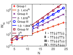
Figure 1: Numbers of states vs the numbers of spins for all groups with representative states for all groups.

The states of both groups must have even numbers of spins. The original (non-inverted) states are characterized by a zero spin projection to the $z$ axis. The zero spin projection corresponds to the filling factor $1/2$ leading to at least two fold degeneracy of all states [49], which is realized for eigenstates of the problem Eq. (1) shifted by the one lattice period with respect to each other, since they cannot be coupled by pair hopping.

The remaining non-translationally invariant states can be represented by states containing at least two odd sequences with oppositely oriented spins. We separate them into two groups including the group III of states having no frozen spins, with conserved projections to the $z$-axis, and group IV of states containing frozen spins as defined in Eq. (37) (for example, third, fourth and fifth spins are frozen in the representative state of the group IV in Fig. 1). The group IV contains the majority of states ($\propto 2^{N}$) including $1.134\cdot 1.7549^{N}$ completely frozen states with all frozen spins, see Appendix B. Localization obviously takes place for the group IV states split into independent blocks by frozen spins. The group III states are mostly localized for the present model Eq. (1) in accord with the imbalance behavior (see Fig. 2).

The states with odd number of spins belong either to the group III or IV depending on the presence of frozen spins Eq. (37) (see Sec. III.5).

III.3 Translational invariance.

Here we prove the translational invariance for the groups I and II and its absence for almost all Krylov’s subspaces in groups III and IV. To prove the translational invariance for the groups I or II consider the product state belonging to these groups with even number of spins in all odd-numbered sequences. Such state is illustrated by the state $A=\{2,3,4,3\}$ defined below as

$$({\rm\mathbf{A}})\overset{1}{{\color[rgb]{1,0,0}\big{\uparrow}}}\overset{2}{{\color[rgb]{1,0,0}\big{\uparrow}}}\overset{3}{{\color[rgb]{0,0,1}\big{\downarrow}}}\overset{4}{{\color[rgb]{0,0,1}\big{\downarrow}}}\overset{5}{{\color[rgb]{0,0,1}\big{\downarrow}}}\overset{6}{{\color[rgb]{1,0,0}\big{\uparrow}}}\overset{7}{{\color[rgb]{1,0,0}\big{\uparrow}}}\overset{8}{{\color[rgb]{1,0,0}\big{\uparrow}}}\overset{9}{{\color[rgb]{1,0,0}\big{\uparrow}}}\overset{10}{{\color[rgb]{0,0,1}\big{\downarrow}}}\overset{11}{{\color[rgb]{0,0,1}\big{\downarrow}}}\overset{12}{{\color[rgb]{0,0,1}\big{\downarrow}}}\rightarrow({\rm\mathbf{B}})\overset{1}{{\color[rgb]{1,0,0}\big{\uparrow}}}\overset{2}{{\color[rgb]{1,0,0}\big{\uparrow}}}\overset{3}{{\color[rgb]{0,0,1}\big{\downarrow}}}\overset{4}{{\color[rgb]{0,0,1}\big{\downarrow}}}\overset{5}{{\color[rgb]{0,0,1}\big{\downarrow}}}\overset{6}{{\color[rgb]{1,0,0}\big{\uparrow}}}\overset{7}{{\color[rgb]{1,0,0}\big{\uparrow}}}\overset{10}{{\color[rgb]{0,0,1}\big{\downarrow}}}\overset{11}{{\color[rgb]{0,0,1}\big{\downarrow}}}\overset{8}{{\color[rgb]{1,0,0}\big{\uparrow}}}\overset{9}{{\color[rgb]{1,0,0}\big{\uparrow}}}\overset{12}{{\color[rgb]{0,0,1}\big{\downarrow}}}\rightarrow$$

$$({\rm\mathbf{C}})\overset{1}{{\color[rgb]{1,0,0}\big{\uparrow}}}\overset{2}{{\color[rgb]{1,0,0}\big{\uparrow}}}\overset{3}{{\color[rgb]{0,0,1}\big{\downarrow}}}\overset{4}{{\color[rgb]{0,0,1}\big{\downarrow}}}\overset{5}{{\color[rgb]{0,0,1}\big{\downarrow}}}\overset{10}{{\color[rgb]{0,0,1}\big{\downarrow}}}\overset{11}{{\color[rgb]{0,0,1}\big{\downarrow}}}\overset{6}{{\color[rgb]{1,0,0}\big{\uparrow}}}\overset{7}{{\color[rgb]{1,0,0}\big{\uparrow}}}\overset{8}{{\color[rgb]{1,0,0}\big{\uparrow}}}\overset{9}{{\color[rgb]{1,0,0}\big{\uparrow}}}\overset{12}{{\color[rgb]{0,0,1}\big{\downarrow}}}\rightarrow({\rm\mathbf{D}})\overset{3}{{\color[rgb]{0,0,1}\big{\downarrow}}}\overset{4}{{\color[rgb]{0,0,1}\big{\downarrow}}}\overset{1}{{\color[rgb]{1,0,0}\big{\uparrow}}}\overset{2}{{\color[rgb]{1,0,0}\big{\uparrow}}}\overset{5}{{\color[rgb]{0,0,1}\big{\downarrow}}}\overset{10}{{\color[rgb]{0,0,1}\big{\downarrow}}}\overset{11}{{\color[rgb]{0,0,1}\big{\downarrow}}}\overset{6}{{\color[rgb]{1,0,0}\big{\uparrow}}}\overset{7}{{\color[rgb]{1,0,0}\big{\uparrow}}}\overset{8}{{\color[rgb]{1,0,0}\big{\uparrow}}}\overset{9}{{\color[rgb]{1,0,0}\big{\uparrow}}}\overset{12}{{\color[rgb]{0,0,1}\big{\downarrow}}}~{}~{}~{}~{}\hskip 1.42271pt$$ (36)

The translational invariance with the period $2$ for these states can be demonstrated considering spin pair hopping starting with the rightmost sequence $k$ in even numbered position having more than one spin ($n_{k}>1$) (spins $10$, $11$, $12$ in the state $A$ in Eq. (36)). If there is only one spin there then another even numbered sequence $k$ should be considered with $n_{k}>1$. One can take the leftmost pair of spins in this sequence and move it to the left until joining the left next neighboring sequence $k-2$ that is possible because $k-1^{st}$ sequence is even (transition $A\rightarrow B\rightarrow C$ in Eq. (36)). Then the leftmost spin pair of $k-2^{nd}$ sequence (spins $3$, $4$) moves left to join $k-4^{th}$ sequence ($C\rightarrow D$). This procedure should be continued until the pair of spins will join the $k^{th}$ sequence from the right (the state $D$ in Eq. (36)). The final state ($D$) is formed by the translation of the initial state ($A$) to the right by two steps. This proves the translational invariance of the associated Krylov subspace and, consequently, eigenstates of the problem.

Using the similar arguments one can give a full description of Krylov subspaces of groups I and II. The states of the group I for $N$ spins and total spin projection $S$ to the $z$ axis for the inverted states (remember that for the group I $N$ must be even and $S$ must be integer) belong to two Krylov subspaces of states made of even sequences with the sequence borders located all either in even or odd positions.

The states and Krylov’s subspaces of the group II can be further characterized using the analysis similar to that in Ref. [38] for non-local integrals of motion. Such analysis is beyond the scope of the present paper targeted to distinguish delocalized, translationally invariant states of groups I and II and almost all localized states of groups III and IV.

Krylov subspaces containing states with both odd- and even-numbered oppositely oriented odd sequences have no translational invariance except for marginal situations including, for instance, Krylov subspaces containing periodic states (e. g. $\{3,3,3,3\}$).

To prove that consider the closest oppositely oriented odd sequences in odd and even positions. They are separated by the even number of even sequences. These sequences can be removed by means of pair hops from each sequence towards the closest odd sequences with the same direction of spins. Since the spin pair located between two odd sequences cannot hop through them the position of this border is conserved within the Krylov subspace.

The position of the boundary between two odd sequences in that configuration is unique and it cannot be modified by the pair hopping because of the spin projection conservation to the $z$ axis. Odd sequences are not transparent for pair hopping because pairs move by two steps only. Therefore adjacent odd sequences confine the spin transport breaking down the translational invariance of corresponding Krylov subspaces. This is not true for the group II states where all odd sequences possess the same spin orientation. Indeed, they can exchange by pairs that can pass through even sequences separating them.

The fixed position of the boundary between neighboring odd sequences in the product state with the minimized number of sequences violates the translational invariance of the Krylov subspace with the only exception of subspaces containing the translationally invariant states composed by self-repeating sets of spins. The simplest translationally invariant states belonging to the group III are given by self repeating sequences $\{2p+1,2p+1,...2p+1\}$ with any integer $p$ [36].

III.4 Frozen spins

The majority of states of the system ($\sim 2^{N}$) belong to the shattered group IV because of the existence of a finite length frozen spin groups [35; 41] in the large number of spins limit. Indeed, if there exist the frozen spin group of a finite length it can be characterized by the formation probability $P_{f}$ per the unit chain length. Consequently, in the large number of spins limit the probability to avoid that group scales approximately as $e^{-P_{f}N}$ suggesting exponentially small weight of states lacking frozen spins,

How are these frozen groups formed? If a sequence is even and at least one of its neighboring sequences possesses more than one spin, then all spins within that even sequence are mobile since the pair of spins from the neighboring sequence can hop through the sequence under consideration shifting all its spins by two (see e. g. $A\rightarrow C$ transition in Eq. (36)). Therefore an even sequence can belong to the frozen set only if its neighboring sequences contain only one spin.

If an odd sequence has both neighbors containing more than one spin it is mobile. However, if one of its neighbors has the only one spin then its edge spin on that side cannot hop until that neighboring sequence changes. Consequently, a single spin sequence surrounded by two odd sequences (see case A below)

$$({\rm\mathbf{A}})~{}\overset{1}{{\color[rgb]{1,0,0}\big{\uparrow}}}\overset{2}{{\color[rgb]{1,0,0}\big{\uparrow}}}\overset{3}{{\color[rgb]{0,0,1}\big{\downarrow}}}\overset{4}{{\color[rgb]{0,0,1}\big{\downarrow}}}\boxed{\overset{5}{{\color[rgb]{0,0,1}\big{\downarrow}}}\overset{6}{{\color[rgb]{1,0,0}\big{\uparrow}}}\overset{7}{{\color[rgb]{0,0,1}\big{\downarrow}}}}\overset{8}{{\color[rgb]{0,0,1}\big{\downarrow}}}\overset{9}{{\color[rgb]{0,0,1}\big{\downarrow}}}\overset{10}{{\color[rgb]{0,0,1}\big{\downarrow}}}\overset{11}{{\color[rgb]{0,0,1}\big{\downarrow}}}\overset{12}{{\color[rgb]{1,0,0}\big{\uparrow}}}\hskip 35.56593pt$$

$$({\rm\mathbf{B}})~{}{\color[rgb]{1,0,0}\big{\uparrow}}{\color[rgb]{1,0,0}\big{\uparrow}}{\color[rgb]{0,0,1}\big{\downarrow}}{\color[rgb]{0,0,1}\big{\downarrow}}\boxed{{\color[rgb]{0,0,1}\big{\downarrow}}{\color[rgb]{1,0,0}\big{\uparrow}}\left[{\color[rgb]{0,0,1}\big{\downarrow}}\underset{\rm\bf even}{\bullet\bullet\bullet}{\color[rgb]{0,0,1}\big{\downarrow}}{\color[rgb]{1,0,0}\big{\uparrow}}\right]_{n}{\color[rgb]{0,0,1}\big{\downarrow}}}{\color[rgb]{0,0,1}\big{\downarrow}}{\color[rgb]{0,0,1}\big{\downarrow}}{\color[rgb]{0,0,1}\big{\downarrow}}{\color[rgb]{0,0,1}\big{\downarrow}}{\color[rgb]{1,0,0}\big{\uparrow}}$$ (37)

forms a simplest frozen set $\{odd,1,odd\}$ with three frozen spins at positions $(5,6,7)$ shown within the box in the state $A$ in Eq. (37). If the set $\{odd,1\}$ is followed by the sequence with an even number of spins it should have the next sequence containing only a single spin to keep spins being frozen. The fragment $\{even,1\}$ can be added an arbitrary number of times ($n$ in Eq. (37), state B) until being terminated by the odd sequence. This is the only way of creating a finite size frozen set of spins just by construction.

Completely frozen states must have each sequence with more than one spin being surrounded by single spin sequences (except for the state of all identical spins). The number of such states belonging to the group IV increases with the number of spins as $1.134\cdot 1.7549^{N}$, see Appendix B.

III.5 States possessing odd number of spins

We cannot invert spins in a periodic chain with an odd number of spins since odd positions become even after passing the period as shown below:

$$(\mathbf{A})\downarrow\uparrow\downarrow\downarrow\uparrow~{}\rightarrow~{}(\mathbf{A}_{1})\downarrow\downarrow\uparrow\uparrow\downarrow,\hskip 22.76228pt$$

$$(\mathbf{B})\overset{1}{\downarrow}\overset{2}{\downarrow}\overset{3}{\downarrow}\overset{4}{\uparrow}\overset{5}{\uparrow}~{}\rightarrow~{}(\mathbf{B}_{1})\overset{1}{\downarrow}\overset{4}{\uparrow}\overset{5}{\uparrow}\overset{2}{\downarrow}\overset{3}{\downarrow}~{}\xcancel{\rightarrow}~{}(\mathbf{B}_{2})\overset{5}{\uparrow}\overset{3}{\downarrow}\overset{1}{\downarrow}\overset{2}{\downarrow}\overset{4}{\uparrow},$$

$$(\mathbf{C})\overset{1}{\downarrow}\overset{2}{\downarrow}\overset{3}{\downarrow}\overset{4}{\uparrow}\overset{5}{\uparrow}\overset{6}{\uparrow}\overset{7}{\uparrow}\overset{8}{\uparrow}\overset{9}{\downarrow}\overset{10}{\downarrow}~{}\rightarrow~{}(\mathbf{C}_{1})\overset{1}{\downarrow}\overset{4}{\uparrow}\overset{5}{\uparrow}\overset{2}{\downarrow}\overset{3}{\downarrow}\overset{6}{\uparrow}\overset{9}{\downarrow}\overset{10}{\downarrow}\overset{7}{\uparrow}\overset{8}{\uparrow}.$$ (38)

In the inverted chain with overturned spins in even positions the state $A$ transforms to the state $B$. According to the rules for the pair hopping in addition to the pair hopping leading to the state $B_{1}$ (the straight chain state $A_{1}$) there is the pair hopping through the border to the state $B_{2}$, which is not permitted for the straight state. This problem can be resolved adding the second chain that is the fully inverted copy of the first chain (see the state $C$ in Eq. (38)). Then the pair hopping should be performed simultaneously for the pair and its copy like it is shown for the transition $C\rightarrow C_{1}$ where the hopping of the pair of spins $2$ and $3$ by two steps to the right is accompanied by the hopping of its inverted copy (spins $(7,8)$) by two steps to the right. There is only one allowed pair hopping from the state $C_{1}$ backwards to the state $C$. Thus this double chain with partially inverted spins have hopping of pairs equivalent to dipole moment conserving transitions in the straight spin chain.

Consequently, one can construct the Krylov subspace in double inverted chain using simultaneous hopping of pairs and their copies shifted by $N$. Similarly to the previous consideration a simultaneous existence of odd sequences in even and odd positions breaks down the translational invariance of the Krylov subspace. It turns out that such sequences exist inevitably in any state of $2N$ spins for an odd number of spins $N$.

Indeed, for an odd total number of spins $N$ at least one sequence containing an odd number of spins must exist. Then its copy with the opposite spin orientation must exist as well in the copy state. Consequently, we have two sequences with odd numbers of spins occupying odd and even positions (because they are of opposite orientations) that contradicts to the requirement for all either odd- or even-numbered sequences to have even numbers of spins, which is the necessary requirement for the translational invariance.

Thus we show that spin states having an odd numbers of spins always have confined spin transport and belong either to the group III if all spins are mobile or the group IV if it contains frozen spins Eq. (37).

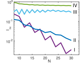
Figure 2: Dependence of average imbalances evaluated within the infinite time limit on the number of spins for different groups (solid lines with the group numbers in the right).

III.6 Group averaged imbalances

Here we consider the connection between the groups, defined in Sec. III.2, and dynamic properties of states belonging to these groups expressed in terms of experimentally accessible imbalance determined by the evolution of the initial product state [65; 2]. The average imbalance for the initial product state $a$ is defined as [2]

$$I_{a}(t)=\frac{\frac{1}{N}\sum_{k=1}^{N}<S_{k}^{z}(t)><S_{k}^{z}(0)>-<S_{k}^{z}>_{*}^{2}}{1/4-<S_{k}^{z}>_{*}^{2}}.$$ (39)

where $<S_{k}^{z}(0)>$ is the projection of the spin $k$ to the $z$ axis in the state $a$, $<S_{k}^{z}(t)>$ is the average projection of this spin to the $z$ axis at time $t$ and $<S_{k}^{z}>_{*}$ is the expectation value for the projection of the spin to the $z$ axis in the ergodic system. With this definition the imbalance should approach zero in the ergodic regime at an infinite time and in the thermodynamic limit of an infinite number $N$ of spins [4]. In the localized regime it should remain constant. The convergence of imbalance to its expectation value in the ergodic, delocalized regime has to be exponential as $N$ approaches infinity.

This criterion is used below to distinguish localized and delocalized states. The delocalized regime is not necessarily ergodic [37] and therefore we discuss the level statistics in the end of the present section.

How to define correctly expectation value $<S_{k}^{z}>_{*}$ in the ergodic regime? In the infinite temperature limit we assume that all states contributing to the eigenstates should be represented equally in this average. Consequently, spin projections should be averaged over the Krylov subspace defined for each given initial state.

It is straightforward to define average spin projections for Krylov subspaces corresponding to the translationally invariant groups I and II for even numbers $Н$ of spins. The Hamiltonian Eq. (1) conserves the total projections of odd and even numbered spins to the $z$ axis ($S_{odd}=\sum_{k=1}^{N/2}S_{2k-1}^{z}$ or $S_{even}=\sum_{k=1}^{N/2}S_{2k}^{z}$, respectively). Then the Krylov subspace averaged projection of spin $k$ to the $z$ axis is given by $2S_{odd}/N$ or $2S_{even}/N$ for odd or even $k$, respectively, due to the translational invaariance of the Krylov subspace with the period $2$. We used this definition of expectation values in Eq. (39) for even number of spins and arbitrarily group of the initial state. For odd number of spins we set the expectation value for the average spin projection equal to its average value $\sum_{k=1}^{N}S_{k}^{z}/N$. With this definition of the spin projection expectations we evaluated group averaged imbalances in the infinite time limit as shown in Fig. 2. The Krylov subspace averaged imbalances for groups III and IV are quite close to those evaluated with spin projection expectation values used in Fig. 2 as illustrated in Fig. 3. Therefore our definition of expectation values is relevant for all states that is important for the analysis of experimental data. Indeed, it is streightforward to evaluate spin projections using the initial states, while the evaluation of Krylov subspace averaged projections can be problematic because of the exponentially large number of states.

The group averaged imbalances represented in Fig. 2 are obtained averaging imbalances for specific state $a$ over all states belonging to a certain group. They are given in an infinite time limit ($I_{\infty}$) [66]. The infinite time limit of imbalance is evaluated numerically expanding the time dependent system wavefunction over the basis of eigenstates $|\alpha>$ with eigenenergies $E_{\alpha}$, obtained using exact diagonalization of the system Hamiltonian, as (remember that we set $\hbar=1$)

$$|\psi(t)>=\sum_{\alpha}<\alpha|a>|\alpha>e^{-iE_{\alpha}t}.$$ (40)

Consequently, the average spin projection at the time $t$ ($<S_{k}^{z}(t)>$) can be expressed as $\sum_{\alpha,\beta}e^{-i(E_{\alpha}-E_{\beta})t}<\alpha|a><a|\beta><\beta|S_{k}^{z}|\alpha>$. In the infinite time limit we leave only terms with $E_{\alpha}=E_{\beta}$, while oscillating terms are averaged out. This yields

$$<S_{k}^{z}(\infty)>$$

$$=\sum_{\alpha,\beta}<\alpha|a><a|\beta><\beta|S_{k}^{z}|\alpha>\delta_{E_{\alpha},E_{\beta}},$$ (41)

where the generalized Kronecker symbol $\delta_{E_{\alpha},E_{\beta}}$ is equal to unity for $E_{\alpha}=E_{\beta}$ and $0$ otherwise.

The infinite time limit is accessible experimentally using time averaged imbalance as demonstrated in Appendix C.

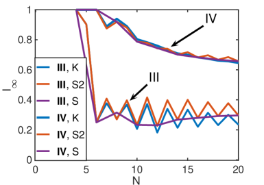
Figure 3: Comparison of average imbalances for groups III and IV with expectation values evaluated for different subspaces. Letter $K$ means Krylov subspace averaging, letters $S2$ means averaging over subspaces with fixed odd and even sublattice spin projections to the $z$ axis for even number of spins, while $S$ means averaging with the fixed total spin projection to the $z$ axis.

The dependence of group average imbalances on the number of spins is consistent with our expectations. The average imbalances approach zero exponentially with increasing $N$ for delocalized states of groups I and II and remains finite for other two groups with increasing $N$.

The convergence of imbalance to its expectation value in Fig. 2 is exponential in the number of spins $N$ for groups I and II as it is expected for the ergodic behavior. However, the additional analysis of the level statistics (to be reported elsewhere) suggests ergodic behavior only for the states belonging to the group II, that is consistent with earlier expectations for the Bethe anzatz integrable nature of the group I states for the present problem Eq. (1). However, the addition of a small amount of quenched disorder should make the system ergodic [67].

The actual imbalance is affected by the Schrieffer-Wolff rotation modifying the definitions of the spin projection operators compared to the minimalist model Fig. 3. However, we expect this effect of order of $(J/F)^{2}$ to be of a minor significance already at $F>3J$.

IV Discussion of the recent experiments [1; 2]: How to observe delocalization at large field gradients?

Here we discuss the spin systems investigated experimentally in Refs. [1; 2] that are similar to those considered in the present work. For a large field gradient $F\approx 2.5J$ a substantial localization was observed in these experiments for all probed initial states in contrast with the expected coexistence of localized and delocalized states. In our opinion this is the consequence of system inhomogeneity due to the open boundaries [1; 2] and the lack of some spin-spin next neighbor interactions in the system, investigated in Ref. [1]. Below we show for both systems that removing inhomogeneity and making them periodic following the receipt of Sec. II.2 one can observe delocalization of states belonging to the groups I and II at arbitrary large field gradient.

IV.1 Interacting qubits within the superconducting quantum processor [1].

Two systems of $16$ and $29$ qubits within the superconducting quantum processor were investigated in Ref. [1]. Both systems can be represented by $XY$ models of interacting spins $1/2$ (qubits) placed into uniformly growing field. For $16$ spins only nearest neighbor interactions were used so the system can be reduced to free fermions [61]. For this system the full Wannier – Stark localization of all states always takes place so we do not consider it.

Thus the system of our interest is formed by $29$ qubits (spins $1/2$) arranged in a chain with the nearest and next neighbor hopping interactions $J_{ij}S_{i}^{+}S_{j}^{-}$ all defined in Fig. S2.A in Supplementary Materials of Ref. [1] with almost identical interactions $J_{ij}$ for a majority of nearest and next neighbor interactions except for several lacking next neighbor interactions. There is no direct interaction between the ends of the chain so the OBC regime is realized. Consequently, at large field gradients the effective Hamiltonian of the system contains static longitudinal fields $h_{k}$ acting on spins, which are generated in the second order of the Schrieffer-Wolff expansion Eq. (6) in the form

$$h_{k}=-\frac{1}{4F}\sum_{l\neq k}\frac{J_{kl}^{2}}{(k-l)}.$$ (42)

These fields are shown in Fig. 4 where they are rescaled by the factor $J^{2}/F$ and compared with four spin hopping amplitude $\Delta$ Eq. (1) rescaled by the factor $J^{3}/F^{2}$. Their relationship in Fig. 4 corresponds to the case of $J=F$. Even in that case a typical field is comparable with the hopping strength, while for larger field gradient $F$ the ratio of generated fields and the hopping amplitude increases proportionally to $F$. Consequently, in this limit the full many-body localization should be naturally expected in agreement with the experimental results [1].

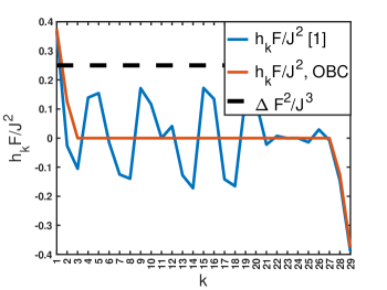
Figure 4: Longitudinal fields vs. the number of spin $k$ generated by means of the Schrieffer-Wolff transformation in the model of Ref. [1] (blue line) and in the OBC model with all identical interactions between nearest and next neighbor spins (red line) compared to the four spin hopping interaction conserving dipole moment (dashed black line).

However, if we set all neighbor and next neighbor interactions equal to each other (leaving other interactions equal to zero as in Ref. [1]) then the field is induced only in the four edge sites of the spin chain, while it is zero in all other sites (see Fig. 4). In this case (referred in Figs. 4 and 5 as the OBC model) delocalization can take place for all spins, except for those at edges, at arbitrarily large field gradient. If in addition the system is made periodic implementing the time-periodic Hamiltonian of Eq. (12), then no longitudinal field exists. In the latter case the states should be separable into localized and delocalized groups in accord with Sec. III.

Here we report the investigation of imbalances in all three models referred as that of Ref. [1], OBC and PBC within the minimalist models represented by the Schrieffer-Wolff expansion up to the third order in $J/F$ for $F\gg J$. Since the number of spins in Ref. [1] is odd ($N=29$) the product states can belong only to groups III or IV. We evaluated average imbalances within the infinite time limit for these groups for all three models choosing initial state randomly and collecting data until the standard deviation of the average imbalance for each group exceeds $0.5$%. We also collected minimum imbalances for all considered states to approach most delocalized states. It is natural to expect that the initial state possessing the minimum imbalance belongs to the Krylov subspace with most delocalized states. Average spin projections in the initial product states were used for spin projection expectation values in the definition of imbalance Eq. (39) similarly to Sec. III.6 for an odd number of spins.

The Monte-Carlo estimate of imbalances has been compared with the exact calculations for the system of $N=20$ spins where it gives quite reasonable estimate both for average and minimum imbalances. This justifies its application to $N=29$ spins.

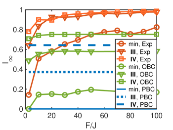
Figure 5: Average infinite time imbalances for groups III and IV and minimum imbalances vs. a field gradient $F$. The results are given for the models of Ref. [1] (Exp), OBC and PBC minimalist models.

Average imbalances for the groups III and IV and minimum imbalances are shown in Fig. 5. The imbalance behavior indicates substantial localization in the model of Ref. [1] with increasing the field gradient $F$ where average and minimum imbalances increase with increasing $F$ approaching the maximum value $1$. This is due to longitudinal fields (see Fig. 4) suppressing delocalization stronger at larger $F$. In OBC and PBC models imbalances are almost or completely field gradient independent because there is no generated longitudinal fields for the majority of spins (OBC) or all spins (PBC) in these models. Yet, finite average imbalances suggests substantial localization of states in both models that is consistent with the nature of the groups III and IV.

The minimum imbalance for the model generated using experimental parameters [1] and at the field gradient $F=2.5J$ is $I_{\rm min}=0.1423$. It is realized for the initial stare $\downarrow\uparrow\uparrow\downarrow\downarrow\uparrow\downarrow\downarrow\uparrow\uparrow\downarrow\downarrow\uparrow\uparrow\downarrow\downarrow\uparrow\downarrow\uparrow\downarrow\downarrow\uparrow\uparrow\downarrow\uparrow\downarrow\uparrow\uparrow\downarrow$. The corresponding eigenstates are partially delocalized, yet representing the minority of states since the average imbalance exceeds $0.6$ (see Fig. 5). Further increase of the field gradient leads to the increase of the minimum imbalance (e. g $I_{min}=0.5$ for $F=8J$) indicating the localization of all states due to generated static fields.

The minimum imbalance for the PBC model $I_{\rm min}=0.27\cdot 10^{-3}$ indicates a substantial delocalization of corresponding states (initial state is $\uparrow\downarrow\downarrow\uparrow\uparrow\downarrow\downarrow\uparrow\downarrow\uparrow\downarrow\uparrow\downarrow\uparrow\uparrow\downarrow\uparrow\downarrow\downarrow\downarrow\uparrow\uparrow\uparrow\downarrow\downarrow\downarrow\uparrow\uparrow\downarrow$). Thus delocalization of a minority of states is possible for the group III states where all spins are mobile. The minimum imbalance for the OBC model at large field gradient realized for the initial state $\downarrow\downarrow\downarrow\uparrow\downarrow\downarrow\uparrow\uparrow\downarrow\downarrow\uparrow\uparrow\uparrow\downarrow\downarrow\uparrow\uparrow\downarrow\downarrow\uparrow\downarrow\uparrow\uparrow\downarrow\uparrow\downarrow\downarrow\uparrow\uparrow$ is around $0.15$. This estimate is approximately consistent with the minimum imbalance estimate $4/29\sim 0.14$ for the fully delocalized state where all spins except for the four spins at the chain boundaries supposes to have time averages close to zero. Therefore, there can be a substantial delocalization for some states of the OBC model. For the minimum considered field gradient $F=2.5J$ the minimum imbalance for that model approaches zero.

Thus delocalization of some states in the system studied in Ref. [1] can be attained in the large field gradient limit by making the spin-spin interactions between nearest and next neighbor spins identical. The delocalization can be further strengthened by means of making the system periodic and using an even numbers of spins as shown in Fig. 2 for the groups I and II.

Our consideration is limited to the minimalist model. The numerical study of more accurate models for the system of $29$ spins is problematic because of the huge number of states involved. Yet we believe that our results remain valid at least qualitatively according to the analysis of Sec. II.3.

IV.2 Trapped ion quantum simulator [2].

Here we examine the chain of $N=15$ spins with the hopping interaction $J_{ij}=1/|i-j|^{1.3}$ placed in a uniformly growing field with the gradient $F$, Eq. (2). This model approximately represents interacting cold atoms investigated in Ref. [2]. Another system of $25$ atoms was also considered there. However, the latter system is too complicated for our consideration because of the very large Hilbert space (over $10^{5}$ states with the total spin $1/2$ and fixed dipole moment $P=0$ modulo $25$). The consideration was still possible for the system of $29$ spins examined earlier, Sec. IV.1, because its effective Hamiltonian possesses a smaller Krylov subspaces due to a short-range interaction there.

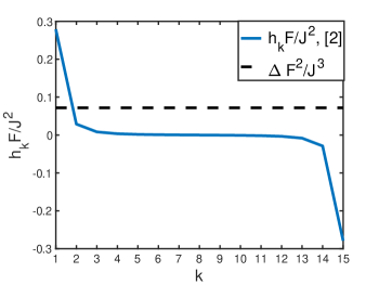
Figure 6: Longitudinal fields vs. the number of spin $k$ generated by means of the Schrieffer-Wolff transformation in the model of Ref. [2] (blue line) compared to the four–spin hopping interaction conserving dipole moment (dashed black line).

Experimentally investigated systems are characterized by open boundary conditions (OBC). Consequently, similarly to Sec. IV.1, there exist static longitudinal fields generated in the second order of perturbation theory Eq. (6), as shown in Fig. 6 where the fields are rescaled by the factor $J^{2}/F$ and compared with four spin hopping amplitude rescaled by the factor $J^{3}/F^{2}$ similarly to that in Fig. 4 in Sec. IV.1. In the case of $J=F$ depicted in Fig. 6, only fields acting on the spins at the edges exceed the four spin hopping amplitude, while for larger field gradient $F$ other fields will be also significant. Eventually in the large field gradient limit $F\rightarrow\infty$ many-body localization of all states should take place in accord with the experimental observations [2] similarly to that for Ref. [1] as it was shown in Sec. IV.1. A different behavior is expected for the periodic model lacking longitudinal fields.

To examine the effect of boundary conditions and the relevance of spin state groups we evaluated imbalances exactly for the OBC Eq. (2) and PBC Eq. (12) models. We use hopping amplitudes $J_{ij}=J/r_{ij}^{1.3}$ as in Ref. [2] with $r_{ij}=|i-j|$ in the OBC model and $r_{ij}=2N|\sin(\pi(i-j)/N)|/\pi$ in the PBC model to make it periodic on a circle. The dependence of group averaged imbalances on the field gradient is investigated for $N=12$ to examine the relevance and applicability of the groups. We also evaluated imbalances for the maximum field gradient $F=2.5J$ used experimentally for the system of $15$ spins and compare the results with the periodic system of $14$ spins at the same field gradient $F=2.5J$.

The division of states into groups is not formally applicable to the power law hopping $J_{ij}$ since in the limit of a large field gradient four spin hopping Eq. (11) can involve arbitrary quartets of spins with transitions conserving dipole moments. However, it can be valid approximately because the dominating hopping is still local due to the fast decrease of its amplitude with the interspin distance. For example the hopping amplitude for the quartet transition $S_{i}^{+}S_{i+1}^{-}S_{i+3}^{-}S_{i+4}^{+}$ of two spin pairs separated by one interatomic distance is less then that for the local quartet $S_{i}^{+}S_{i+1}^{-}S_{i+2}^{-}S_{i+3}^{+}$ by almost a factor of $10$ ($8.0$).

It is not clear whether the power-law hopping within the parent model would lead to the inevitable localization breakdown in the infinite number of spins limit. According to the preliminary analysis, the hopping $1/r^{1.3}$ in the case of the strong field gradient does not inevitably lead to all state delocalization as in the models of Refs. [68; 69; 70; 71; 72; 57]. Localization can be unstable for interaction decreasing slower with the distance. Particularly, the recent work [73] reports the number of interesting behaviors in the Stark MBL problem in the case of infinite range distant independent transverse interactions that awaits the proper interpretation and experimental verification. It is not clear whether the ergodic spot arguments [74] are applicable to the present problem as well because of the lack of quenched disorder.

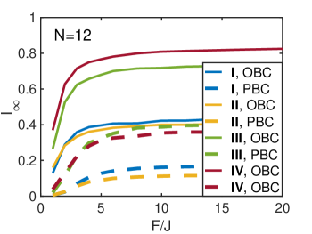
Figure 7: Group averaged imbalance for the periodic and open boundary condition realizations of the system of Ref. [2] vs. the field gradient for $N=12$.

To examine the applicability of the group concept to the system of interest we evaluated imbalances for different initial states and average them over initial state groups for $N=12$. The infinite time limit of group averaged imbalances is shown in Fig. 7 for the system with open boundary conditions (OBC) corresponding to the experiment and the periodic system for $12$ spins. In both cases imbalances are distinguishable for different groups already for $F>2J$. This domain includes the experimentally probed field gradients $F\leq 2.5J$. As noticed in Sec. II.2 the dependence of imbalance on the field gradient saturates at $F\geq 4J$. For the OBC problem imbalance slowly increases with the field gradient due to the localization effect of the longitudinal field induced by the boundaries (see Fig. 6).

The behavior of average imbalances is qualitatively similar to that for the previously considered $29$ spins with a short-range interactions (see Fig. 5). Initial states of the group IV correspond to larger imbalances compared to the states of the group III in accord with our expectations. For OBC systems the average imbalance increases with increasing the field gradient $F$ towards its maximum value of $1$. The minimum imbalance also increases with $F$ indicating localization of all system states.

For the experimentally relevant OBC model of $15$ spins and $F=2.5J$ the minimum imbalance $I_{\rm min}=0.1364$ is found for the initial state $\downarrow\downarrow\uparrow\uparrow\downarrow\uparrow\downarrow\downarrow\downarrow\uparrow\uparrow\downarrow\uparrow\downarrow\uparrow$. The average imbalances for the groups III and IV are given by $0.5221$ and $0.6787$, respectively. This observation suggests the localization of the majority of states in a sharp contrast with the PBC problem for $N=14$ and $F=2.5J$. Group average imbalances for this problem are given by $0.055$, $0.04$, $0.088$, $0.1877$ for the groups I - IV, respectively. Thus the minimum imbalance for the OBC problem is comparable to the averaged imbalance for the most localized group IV for the PBC problem.

This observation suggests delocalization of states for the first three groups and localization of most of states belonging to the fourth one. It is consistent with that for the minimalist model Eq. (1) except for the group III. However, since there exists non-local hopping this observation is approximately consistent with that in Appendix II (Fig. 10). It was shown there that the addition of the fourth order non-local interaction suppresses localization of states of the group III for a field gradient $F<25J$ and even numbers of spins. Consequently, the system containing even numbers of interacting spins with periodic boundary conditions is most suitable to investigate coexistence of localization and delocalization.

V Discussions and Conclusions

Here we summarize the results of the present work and compare them with other work [38; 36; 37; 41] where the composite blocks (pseudospins, dipoles, defects) were introduced to characterize dipole moment conserving spin dynamics. The results can be divided into three parts discussed separately including the classification of Krylov subspaces for the minimalist model (Sec. V.1), understanding spin dynamics in different groups of Krylov subspaces (Sec. V.2) and the application of these findings to existing experiments (Sec. V.3).

V.1 Understanding Krylov subspaces

The visually transparent consideration of spin dynamics in the minimalist periodic dipole moment conserving (modulo $N$) model for the chain of $N$ spins $1/2$ Eq. (1) has been proposed using inverted spin chain with all even numbered spins overturned about $x$ axis by the angle $\pi$. Then the spin transport for even numbers of spins can be represented as hops of pairs of identically oriented spins by two chain periods to the right or to the left. This representation is used to separate all product states and associated Krylov subspaces into four groups based on the parity of identically oriented spin sequences.

V.1.1 Groups of states

The inverted chain states belonging to the group I are composed by the only even sequences (see Fig. 1). Corresponding Krylov subspaces are translationally invariant. Consequently, eigenstates are delocalized. Their dynamics is characterized by the Bethe anzatz integrable anisotropic Heisenberg model for the pseudospins $1/2$ created from adjacent spin pairs similarly to Refs. [48; 36].

The inverted states belonging to the group II have even number of spins in all sequences of adjacent spins oriented either upwards or downwards, while the oppositely oriented sequences must have at least one sequence with more than one spin. Corresponding Krylov subspaces are translationally invariant. Eigenstates belonging to this group are delocalized and we expect them to be ergodic based on the preliminary analysis of the level statistics.

Several Krylov subspaces composed by specific combinations of pseudospins and dipoles belonging to the group II and possessing delocalized eigenstates were identified in Ref. [37]. The transport visualization using inverted lattice permitted us to move further and identify all translationally invariant subspaces thus generalizing the previous work.

The inverted states possessing both upwards and downwards oriented sequences with odd numbers of spins and systems with odd numbers of spins are characterized by non-translationally invariant Krylov subspaces with marginal exceptions of subspaces containing translationally invariant product states, considered in Ref. [36]. These states can be separated into two groups including the group III of states with all mobimle spins and group IV, of states possessing ifrozen spins. All spin sets containing frozen spins are identified.

V.1.2 Numbers of states

The numbers of states belonging to all groups increase exponentially with the numbers of spins $N$. We evaluated this dependence analytically using the generating function method. The number of states increases with the number of the group. The majority of states belong to the group IV.

V.1.3 Integrals of motion

It is possible to identify a number of conserving quantities similarly to Ref. [38] where such quantities were considered for the dipole moment conserving transport in the spin $S=1$ chain. This include for instance the number of spin sequences within the representative product state containing an odd number of spins or the parity of the numbers of spins at odd sequence boundaries (the leftmost spin is always odd, while the rightmost spin is always even or vice versa). In the present work we do not attempt to identify all such integrals of motion concentrating more on the localization problem. Yet below in Sec. V.2 we recognize their significance for understanding spin dynamics.

V.1.4 Possible extension of the arguments to the spin $S=1$ case.

Visualization of spin dynamics within the inverted lattice permits us to represent it as moving vehicles, composed by pairs of adjacent, identically oriented spins, within the environment of the oppositely oriented spins. Similarly, for the minimalist dipole moment conserving spin $1$ problem [35] one can introduce such vehicles made of adjacent spins with opposite projections $\pm 1$. Then these vehicles can move freely within the environment of the spins with the zero projection.

It can be shown (we leave the prove to the readers) that with marginal exceptions the product states forming translationally invariant Krylov subspaces must have spins with the projections $S^{z}=\pm 1$ arranged in the way that each spin with a projection $S^{z}=\pm 1$ has at least one of the two neighboring spins with $|S^{z}|=1$ having the opposite projection $S^{z}=\mp 1$ (that spin can be separated from the given spin by an arbitrary number of spins with the zero projection). Further extensions of theory to more complicated models can be possibly developed, which is beyond the scope of the present work.

V.2 Localization and delocalization of states in different groups. Connection to the parent model.

It is quite natural to expect delocalization of eigenstates belonging to the translationally invariant groups I and II and localization for the states of the group IV possessing the immobile spins. These expectations are fully confirmed by the investigation of the infinite time imbalances. The study of imbalances also shows the localization of almost all states belonging to the group III lacking translational invariance but with all mobile spins.

The model considered in Refs. [36; 37; 41] is different from Eq. (1) because it does not include the longitudinal part containing $S^{z}$ operators. Remember that this part of the Hamiltonian is the outcome of generalized Schrieffer Wolff expansion of the parent XY model, which makes our model more relevant experimentally. To the best of our knowledge in other systems the strong longitudinal interaction is always unavoidable.

To compare system dynamics in two different models we evaluated average imbalances for all groups of states for the model of Refs. [36; 37; 41]. It turns out that the imbalances behave nearly identically for all groups except for the group III, where the ergodic behavior is found in contrast to the localization in the model Eq. (1), considered in the present work.

What is the origin of this difference? In our opinion the longitudinal interaction acts as a quasi-static disorder, localizing spin dynamics. The static nature of disorder can be the consequence of the conserving quantities (cf. Ref. [38]) including the number of odd sequences and positions of their borders that can occupy limited number of places due to the translational invariance breakdown. It is not clear whether this localization survives for group III states in a thermodynamic limit of an infinite system. At least no signature of localization breakdown is seen in Fig. 2 up to $N=30$.

The localizing effect of the longitudinal interactions should be even stronger in other systems including the fractional quantum Hall problem in the thin-torus limit [48; 49; 50; 36] and the anisotropic Heisenberg model with nearest neighbor interactions subjected to a uniformly growing field in a large field gradient limit [41; 59; 60]. In both limits justifying the transverse interaction in the form of Eq. (1) there exist longitudinal interactions exceeding the transverse interaction by the expansion parameter. This should increase the strength of static disorder and the localization trend. Consequently, the present model is expected to be most delocalized, that justifies its experimental and theoretical considerations.

The concept of the groups of states is extendable at least qualitatively to the parent models with time periodic Hamiltonians that can be used to realize the minimalist model experimentally for the large field gradient $F$. It is possible that localization survives there for $F>J$ because of the quasistatic disorder induced by some integrals of motion including for example the approximately conserving dipole moment. This expectation is consistent with the recent observation of Stark gauge protection [75], where the disorder free localization in several quantum gauge theory realizations has been stabilized by the uniformly growing potential in spite of the presence of gauge-breaking interactions.

V.3 Interpretation of experiments and suggestion of their advancement

The localization observed experimentally in Refs. [1; 2] for the large field gradient $F\sim 2.5J$ turns out to be the consequence of the boundaries and lack of certain interactions in Refs. [1]. This issue can be resolved using the periodic spin chain under action of a time–varying Hamiltonian suggested within the present work. Then the system becomes translationally invariant and it should show a full diversity of behaviors depending on the group of the initial state.

The initial product states possessing the minimum imbalances are determined for various experimental settings. It can be worth to probe these substantially delocalized regimes experimentally.

.

Appendix A Applicability of the main approximation

Here we in greater detail the relevance of the minimalist model for characterizing system dynamic. The minimalist model periodic in time and space is derived in the main text using the generalized Schrieffer-Wolff transformation of the time periodic $XY$ model subjected to the uniformly growing field as the first non-vanishing third order term of the effective Hamiltonian expansion in the ratio of interspin interaction $J$ and field gradient $F$ (see Sec. II.B of the main text). This expansion should be valid at sufficiently large field gradient $F>F_{c}$, where the critical field gradient can depend on the number of spins $N$.

In Sec. II.C the conservative and liberal approaches to the estimate of $F_{c}$ are suggested. The conservative estimate requiring the accurate estimate of eigenstate energies within the minimalist model results in exponentially large (in $N$) field $F_{c1}\sim J2^{N/2}$. The liberal approach requiring the convergence of the Schrieffer-Wolff expansion suggests $F_{c2}\sim J$.

Below we analyze the convergence of the generalized Schrieffer-Wolff transformation deriving the fourth order correction to the effective Hamiltonian in Sec. A.0.1 and verifying the convergence of the generalized Schrieffer-Wolff transformation in Sec. A.0.2. Then eigenstate energies obtained using the minimalist model and corrected Hamiltonian are compared to each other in Sec. A.0.3. This comparison results in the estimate of the critical field gradient $F_{c}$ approximately consistent with the conservative estimate. In addition we compare average imbalances for different groups of initial states evaluated using the minimalist model and the original time periodic problem. This study shows that the imbalance behavior for the minimalist model is qualitatively consistent with the exact system already for $F>F_{c2}$ though the quantitative agreement of two results for localized states of the third and fourth groups requires $F>F_{c1}$.

All comparisons are performed for the $XY$ model with nearest and next neighbor interactions different from zero and identical to each other similarly to the experimentally investigated system in Ref. [1]. We set both interactions equal to $J$.

A.0.1 The fourth order correction to the effective Hamiltonian.

The fourth order correction is considered to validate the relevance of the minimalist model and the generalized Schrieffer-Wolff transformation. It consists of two contributions including the fourth order contribution from the Baker-Campbell-Hausdorff-Dynkin formula $\widehat{H}_{4a}$ and the higher order in $F^{-1}$ Schrieffer-Wolff transformation contribution $\widehat{H}_{4b}$ originated from the second order transverse interaction, not conserving dipole moment, emerging similarly to the one for the OBC problem (see Eq. (7) in Sec. II.1 in the main text) that can be written as

$$\widehat{H}_{2offd}=-\sum_{j,k~{}=l}2A_{jk}A_{lj}e^{2\pi i(k-j)/N}S_{j}^{z}S_{l}^{+}S_{k}^{-}+\sum_{j~{}=m,k}2A_{jk}A_{km}e^{2\pi i(k-j)/N}S_{k}^{z}S_{j}^{+}S_{m}^{-}.$$ (43)

Its contribution to the effective Hamiltonian can be derived introducing operators $\widehat{S}_{2}$ and $\widehat{S}_{2mod}$ similarly to Sec. II.2 (see Eq. (44) below).

Then the fourth order correction to the effective Hamiltonian can be expressed as (cf. Eq. (25))

$$\widehat{V}_{4}=\left[\widehat{H}_{4a}+\widehat{H}_{4b}\right]_{P},$$

$$\widehat{H}_{4a}=\frac{i}{8\tau_{F}}[\widehat{S}_{mod},[\widehat{S}_{mod},[\widehat{S}_{mod},\widehat{S}_{1}]]]+\frac{i}{12\tau_{F}}[\widehat{S}_{1},[\widehat{S}_{mod},[\widehat{S}_{mod},\widehat{S}_{1}]]]$$

$$+\frac{i}{24\tau_{F}}[\widehat{S}_{mod},[\widehat{S}_{1},[\widehat{S}_{mod},\widehat{S}_{1}]]]+\frac{i}{24\tau_{F}}[\widehat{S}_{1},[\widehat{S}_{1},[\widehat{S}_{mod},\widehat{S}_{1}]]],$$

$$\widehat{H}_{4b}=\frac{1}{2}[\widehat{S}_{2mod},\widehat{H}_{2offd}],$$

$$\widehat{S}_{2mod}=\frac{1}{16F}\sum_{j\neq l,k}\frac{2\pi i(j+l-2k)J_{jk}J_{kl}S_{k}^{z}S_{j}^{+}S_{l}^{-}}{2NF(j-k)(l-k)}\frac{e^{2\pi i\frac{j-l}{N}}}{1-e^{2\pi i\frac{j-l}{N}}}.$$ (44)

Remember that the subscript $P$ means that the only terms conserving dipole moment $P$ (modulo $N$) are left.

A.0.2 Convergence of the perturbation series.

Here we investigate the convergence of the expansion of the effective Hamiltonian defined by Eq. (16) in the main text. To validate the expansion convergence we compare the third and fourth order approximations to the effective Hamiltonian with the results of the exact diagonalization of the evolution matrix Eq. (13) that can be performed at relatively small numbers of spins $N\leq 15$.

The target Hamiltonian $\widehat{H}_{eff}$ can be considered in the third order approximation referred as the minimalist model and in the fourth order approximation with the fourth order term Eq. (44) added to the minimalist model Hamiltonian., The fourth order approximation is referred as the improved model. The minimalist and improved models are compared with the results of the exact diagonalization of the evolution matrix. Remember that here and in the next section all calculations are performed for the parent $XY$ model with nearest and next-neighbor interactions $J_{1}$ and $J_{2}$. We also set $J_{1}=J_{2}=J$ similarly to the interactions in Ref. [1].

To compare the approximate and exact models we performed exact diagonalization of the minimalist and corrected model Hamiltonians, and exact diagonalization of the evolution matrix (see Eq. (13) in the main text). Its eigenvalues are complex numbers $z_{i}$ with absolute value unity as it has to be for the unitary matrix. According to the definition off the effective Hamiltonian (see Eq. (16) in the main text) logarithms of those numbers for the specific eigenstate $a$ possessing the dipole moment $P_{a}$ can be expressed as

$$\ln(z_{i})=-i\tau_{F}(-FP_{a}+E_{a*}),$$ (45)

where $E_{a*}$ is the eigenenergy of the corresponding state $a$ of the effective Hamiltonian $\widehat{H}_{eff}$. This definition makes sense only for sufficiently large field gradient $F\gg J$. The dipole moment is approximately conserved under this condition. It turns out that already for $F>2.5J$ ($N\leq 14$) imaginary parts of eigenvalue logarithms form $N$ well separated groups corresponding to certain dipole moments (mod $N$). Consequently, target energies $E_{a*}$ are clearly identifiable for each dipole moment.

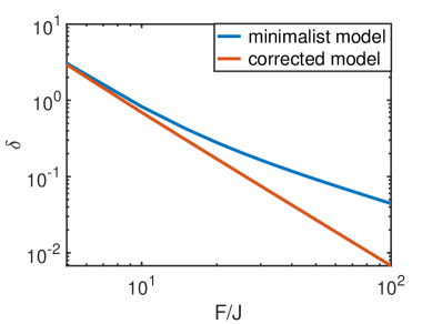
Figure 8: Relative deviation Eq. (46) of eigenstate energies evaluated within the minimalist and corrected models from exact eigenenergies.

Then we compare these energies with eigenenergies of the effective Hamiltonians of the minimalist and improved models. To compare eigenenergies we evaluated the relative deviation $\delta$ of two ordered sets of eigenenergies, which is defined as

$$\delta=\frac{1}{Z}\sum_{i=1}^{Z}\frac{(E_{i,1}-E_{i,2})^{2}}{\delta E^{2}},$$ (46)

where $Z$ is the total number of eigenstates, $E_{i,1}$, $E_{i,2}$ are eigenenergies of the state $i$ obtained using methods $1$ and $2$ and $\delta E$ is the average energy splitting between adjacent energy levels, which was calculated using the most accurate approximation.

Calculations of relative deviations at different field gradients $F$ show that the deviations of the minimalist and improved models from the exact results scale with $F$ as $1/F$ and $1/F^{2}$, respectively, as illustrated in Fig. 8 for the states of $N=12$ spins with a zero total spin projection to the $z$ axis and zero dipole moment, $P=0$ (mod $N$). Calculations for other states show a similar behavior. Consequently, the suggested expansion of the effective Hamiltonian converges at large field gradients $F$, which proves its relevance.

A.0.3 Relevance of the main approximation.

The Hamiltonian of the minimalist model considered in the main text represents the first non-vanishing term in the effective Hamiltonian expansion in $JF^{-1}$ Eq. (28). This approximation should be valid at sufficiently large field gradient $F>F_{c}$. Here we estimate the minimum gradient $F_{c}$ where this approximation is still applicable by comparing energy levels Eq. (46) and imbalances (Eq. (39) in the main text) calculated within this approximation (minimalist model of Eq. (1)) and with the fourth order correction of Eq. (44) added (improved model).

Eigenenergies obtained using two different approaches are compared using Eq. (46) for even numbers of spins $10\leq N\leq 18$ and field gradients $5<F<100$. The results for states with zero spin projection to the $z$ axis and minimum absolute value of the dipole moment ($P=0$ for $N=12$, $16$ and $P=0.5$ for $N=10$, $14$, $18$) are reported in Fig. 9.

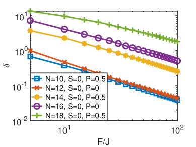
Figure 9: Relative deviation of eigenenergies Eq. (46), evaluated within the minimalist and corrected models, from each other.

We set the formal criterion for the validity of the minimalist model to be $\delta=1$ in Eq. (46). According to this criterion one can estimate $F_{c}/J\approx 5$ for $N=10$ and $12$, $F_{c}/J\approx 30$ for $N=14$, $F_{c}/J\approx 60$ for $N=16$ and $F_{c}/J>100$ for $N=18$. The observed trend for largest numbers of spins is approximately consistent with the conservative estimate of the crossover field gradient obtained in the main text. One can approximately describe that crossover as

$$F_{c1}(N)\approx 0.25\cdot 2^{N/2}J,$$ (47)

where the factor $0.25$ is chosen to satisfy the condition $\delta\approx 1$ in Fig. 9 for $N=16$.

The minimalist model Eq. (1) can have a wider applicability domain since it can leave average properties (e. g. imbalances) unchangeable in spite of large shifts of energy levels. To partially address this concern we consider the difference of imbalances evaluated in the Minimalist Model and in the original time periodic model (Eq. (12) in the main text). Both imbalances are evaluated within the infinite time limit. In both cases we use the most straightforward definition of imbalance (see Eq. (39) in the main text) defining the spin projection expectation values to be equal to average spin projection to the $z$ axis since our goal here is to examine the relevance of the perturbation theory.

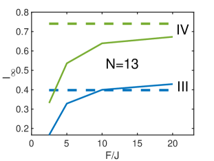
(a)

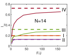
(b)

Figure 10: Group averaged imbalance dependence on the field gradient for $N=13$ (a) and $N=14$ (b). Group is indicated by the Roman number at the right side of the graph. Dashed lines show imbalances evaluated within the minimalist model.

In Fig. 10 the comparison of imbalances evaluated within two models is reported for $N=13$ and $N=14$. Dashed lines show the results for the MM model Eq. (1), which are independent of the field gradient, while solid lines show the results for the original time-periodic model Eq. (12).

Obviously, the minimalist model is not applicable at $F\sim J$ where imbalances are approximately group independent. As it is shown in Fig. 10 the remarkable difference between imbalances evaluated for different groups is already seen at $F=2.5J$. The field gradient dependence of imbalances for groups I and II for $N=14$ and all groups for $N=13$ saturates at around $F\sim 5J$. This is consistent with the liberal criterion $F_{c}\sim J$.

The average imbalances for groups III and IV and $N=14$ reach the minimalist model limit at larger fields $F\sim 40J$ that is consistent with the conservative estimate Eq. (47). Yet for the group IV imbalance exceeds other group imbalances and shows the localization trend already for $F\geq 5J$, while the states of group III can be delocalized for $F<40J$. The similar difference between even and odd size behaviors is seen for larger numbers of spins $N=15$ and $16$ as well.

Appendix B Calculation of numbers of states in different groups.

Here we report the analytical calculations of the numbers of states belonging to the groups II (Sec. B.1) and III (Sec. B.3) using generating function method, while the number of states belonging to the group I ($2\cdot 2^{N/2}$) is given in the main text and the number of states belonging to the group IV approaches the total number of states $2^{N}$. These results are summarized in Fig. 1 in the main text. Also the numbers of states with all frozen spins as a function of the total number of spins is evaluated in Sec. B.2 (this number is also quoted in the main text).

B.1 Counting group II states.

According to the main text the states of group II can be represented by states having even numbers of sequences with either all odd or all even-numbered sequences containing even numbers of spins. Each state must have at least one odd sequence to be distinguished from group I states having all even sequences. Also completely frozen states having either all odd or all even-numbered sequences containing only one spin should be excluded.

States of periodic system belonging to the group II can be distinguished by states of the first and last ($N^{th}$) spins as shown below

$$({\rm\mathbf{A}})~{}\uparrow\uparrow\downarrow\uparrow\uparrow\uparrow\uparrow\downarrow\downarrow\downarrow,~{}~{}~{}({\rm\mathbf{B}})~{}\uparrow\downarrow\uparrow\uparrow\uparrow\uparrow\downarrow\downarrow\downarrow\uparrow.$$ (48)

The states of the type $A$ has first and last spins different, while they are identical for the states of the type $B$ representing the circular shifted state $A$. It is more convenient to calculate first the number of states of the type $A$ and then calculate the number of states of the type $B$ representing them in terms of the states of the type $A$ of the smaller size ($8$ spins in the three internal sequences within the state $B$ in Eq. (48)) with the remaining sequence being added to both sides.

We begin with the calculation of the number of states of the type $A$ having even number of sequences (because the first and last spins are opposite to each other) and having even numbers of spins either in all odd or even-numbered sequences. This definition includes all states of the group I containing only even sequences and fully frozen states belonging to the group IV having a single spin in all sequences in odd or even-numbered positions. They will be excluded from the final answer.

Let $W_{N}^{oo}$ and $W_{N}^{eo}$ be the numbers of states of $N$ spins containing odd or even numbers of sequences, respectively, and having all odd-numbered sequences containing even numbers of spins (e. g. states with $N=9$ represented as $(2,5,2)$ or $(2,3,2,2)$ treated as with the open boundary conditions, i. e. distinguishing the first and the last sequences). Similarly, $W_{N}^{oe}$ and $W_{N}^{ee}$ are the numbers of states of $N$ spins containing odd or even numbers of sequences, respectively, having all even-numbered sequences containing even numbers of spins. Then the state of $N>0$ spins can be obtained from the smaller state by means of adding the sequence of identical spins to the right with their projections opposite to those in the last sequence. We assume no sequences with negative numbers of spins and one sequence with $0$ spins.

The states with $N$ spins, having odd numbers of sequences and all odd-numbered sequences possessing even numbers of spins can be generated from the states having even numbers of sequences and even numbers of spins in odd-numbered sequences by means of adding one more sequence (to the right), having even numbers of spins $2k$ ($k=1,2,3,...$). If $N$ is even this state can be also obtained as one of two states of all spins oriented upwards or downwards added to the zero spin state. Formally this condition can be written as

$$W_{N}^{oo}=\sum_{k=1}^{\infty}W_{N-2k}^{eo}(1+\delta_{N-2k,0}),$$ (49)

where $\delta_{ab}$ is the Kronecker symbol.

The states of $N$ spins, having even numbers of sequences and all odd-numbered sequences possessing even numbers of spins can be generated from the states having odd number of sequences and even number of spins in odd-numbered sequences by means of adding one more sequence, having any numbers of spins $k>0$. Consequently, we get

$$W_{N}^{eo}=\sum_{k=1}^{\infty}W_{N-k}^{oo}+\delta_{N0}.$$ (50)

The last term $\delta_{N0}$ in the right hand side of Eq. (50) reflects the fact that there is one state with even number zero of sequences for $N=0$.

Using similar arguments one can obtain equations for state numbers $W_{N}^{oe}$, $W_{N}^{ee}$ having odd or even numbers of sequences with even sequences in even-numbered positions in the form

$$W_{N}^{oe}=\sum_{k=1}^{\infty}W_{N-k}^{ee}(1+\delta_{N-k,0}),~{}W_{N}^{ee}=\sum_{k=1}^{\infty}W_{N-2k}^{oe}+\delta_{N0}.$$ (51)

The number of states $W_{A}(N)$ for $N$ spins in sequences of the type $A$ in Eq. (48) is the sum of two out of four above defined numbers for total even number of sequences , i. e. $W_{A}(N)=W_{N}^{eo}+W_{N}^{ee}$.

The solution of all equations can be found using generating functions defined as

$$w_{ab}(x)=\sum_{k=0}^{\infty}W_{N}^{ab}x^{N}.$$ (52)

Eqs. (49), (50), (51) can be rewritten for these generating functions as

$$w_{oo}=\frac{x^{2}}{1-x^{2}}w_{eo}+\frac{x^{2}}{1-x^{2}},~{}w_{eo}=\frac{x}{1-x}w_{oo}+1,$$

$$w_{oe}=\frac{x}{1-x}w_{ee}+\frac{x}{1-x},~{}w_{ee}=\frac{x^{2}}{1-x^{2}}w_{oe}+1.$$ (53)

The numbers of interest ($W_{A}(N)$) are defined by the coefficients of the power series expansion

$$w_{A}(x)=\sum_{N=0}^{\infty}W_{A}(N)x^{N}=w_{eo}(x)+w_{ee}(x)-w_{e}(x),$$ (54)

where $w_{e}(x)$ is the generating function for the number of states of $N$ spins composed by an even number of sequences all having even numbers of spins $w_{e}(x)=\sum_{N}W^{e}_{N}x^{N}$. It has to be subtracted because these states are included twice both into numbers $W_{N}^{eo}$ and $W_{N}^{ee}$.

The functions $W^{e}_{N}$, $W^{o}_{N}$ representing the numbers of states composed by even or odd numbers of sequences containing even numbers of spins can be evaluated also using generating function method. Their generating functions are given by

$$w_{o}(x)=\frac{2x^{2}(1-x^{2})}{1-2x^{2}},~{}~{}w_{e}(x)=\frac{2x^{4}}{1-2x^{2}}.$$ (55)

The sum $w_{o}(x)+w_{e}(x)$ yields $1/(1-2x^{2})$ which is the generating function for the number of spin pair states $2^{N/2}$.

Solving Eqs. (53) we get

$$w_{A}(x)=2+\frac{4x^{3}}{1-x+x^{2}}-\frac{2x^{4}}{1-2x^{2}};$$ (56)

Using the power serious expansion (it is straightforward after the partial fraction expansion of the answer) we got the numbers of states of the type $A$ for $N>0$ in the form $(N\geq 2)$

$$W_{A}(N)=8\frac{\sqrt{5}}{5}\left[\frac{\sqrt{5}-2}{\sqrt{5}-1}\left(\frac{\sqrt{5}+1}{2}\right)^{N}-(-1)^{N}\frac{\sqrt{5}+2}{\sqrt{5}+1}\left(\frac{\sqrt{5}-1}{2}\right)^{N}\right]-2^{N/2}/2+\delta_{N,2}.$$ (57)

Consequently, in a limit of a large number of spins one can use the exponential asymptotic behavior $W_{A}(N)\propto\lambda_{min}^{-N}$, where $\lambda_{min}=(\sqrt{5}-1)/2\approx 0.618$ is the root of the denominators in Eq. (56) possessing the minimum absolute value. This exponential asymptotic is valid for the whole number of states in group II since it should not depend on boundaries as we will see below. Subtraction of group I states will not affect this behavior because their number increases with $N$ slower (as $2^{N/2}\approx 1.41^{N}$).

To evaluate the number of states of the type $B$ one can represent each of them as the state of the type $A$ of the smaller size $N-z$ and consider all $z-1$ ways of appending the additional sequence ($(2k-1)(W_{N-2k}^{oo}+W_{N-2k}^{oe}-W_{N-2k}^{o})$ for even length $z=2k$ of the additional sequence or $2kW_{N-2k-1}^{oo}$ for its odd length $z=2k+1$) for all possible numbers $z$. The number of states with odd number of sequences all containing even numbers of spins is subtracted from the definition to avoid including it twice.

Then one can express the number of states of the type $B$ as

$$W_{B}(N)=\sum_{k=1}^{\infty}\left[(2k-1)(W_{N-2k}^{oo}+W_{N-2k}^{oe}-W_{N-k}^{o})+2kW_{N-2k-1}^{oo}\right].$$ (58)

The associated generating function $w_{B}(x)$ can be expressed as

$$w_{B}(x)=(w_{oo}(x)+w_{oe}(x)-w_{o}(x))\frac{x^{2}+x^{4}}{(1-x^{2})^{2}}+w_{oo}(x)\frac{2x^{3}}{(1-2x^{2})}.$$ (59)

To find the total number of states belonging to the group II we need to add both contributions $w_{A}(x)$ and $w_{B}(x)$ found above and subtract all states of the group I having the number $2\cdot 2^{N/2}-4$ in accordance with the main text and fully frozen states $W_{N}^{II,im}$ evaluated below in Eqs. (68) and (69). Then the generating function for the total number of states within the group II takes the form

$$w_{II}(x)=w_{A}(x)+w_{B}(x)-\frac{2}{1-2x^{2}}+\frac{4}{1-x^{2}}-w_{II,im}=\frac{2(4x^{5}+12x^{4}-12x^{2}+3)}{2x^{5}+4x^{4}-x^{3}-4x^{2}+1}-\frac{2x^{3}(2+x)}{1-2x^{2}}.$$ (60)

The expansion of the generating function $w_{II}(x)$ into power series results in the exact answer below for the numbers of states belonging to the group II

$$W_{N}^{II}=2\left[\left(\frac{\sqrt{5}+1}{2}\right)^{N}+(-1)^{N}\left(\frac{\sqrt{5}-1}{2}\right)^{N}-2^{N/2}\left(\frac{5+2\sqrt{2}}{4}+(-1)^{N}\frac{5-2\sqrt{2}}{4}\right)+\delta_{2,N}+2\right].$$ (61)

This answer is applicable only for even numbers of spins $N$.

B.2 Counting completely frozen states.

Completely frozen states are formed by spin sets consisting of all identical spins (trivial case of two states) or they must have each sequence containing more than one spin being surrounded by sequences containing only one spin. To solve this problem for a periodic system we can use the approach of Eq. (48) splitting all states into types $A$ and $B$ based on the first and the last spins. Then the total number of states of interest can be expressed as

$$W_{N}^{im}=W_{N}^{A}+W_{N}^{B},~{}W_{N}^{B}=\sum_{k=2}^{\infty}Y_{N-k}^{o1}(k-1),$$ (62)

where $W_{N}^{A}$ is the number of frozen states of type $A$ with $N$ spins, $W_{N}^{B}$ is the number of $N$ spin frozen states of type $B$ with $N$ spins and $Y_{N}^{o1}$ is the number of frozen states containing an odd number of sequences with first and last sequence containing only one spin. There is no other way to compose the state of type $B$ avoiding mobile spins in the edge sequence. One can reexpress Eq. (62) in terms of the corresponding generating functions as (cf. Eq. (60))

$$w_{im}=w_{A}+\frac{x^{2}}{(1-x)^{2}}y_{o1}.$$ (63)

To find numbers of specific states we introduce the functions $Y_{N}^{o1}$, $Y_{N}^{o}$, $Y_{N}^{e1}$, $Y_{N}^{e}$ and $W_{N}^{o1}$, $W_{N}^{o}$, $W_{N}^{e1}$, $W_{N}^{e}$. The states denoted by the letter $Y$ begins with the sequence containing one spin, while the states denoted by the letter $W$ have the initial sequence of more than one spins. Superscripts $o$ or $e$ mean that the states contain odd or even numbers of sequences, respectively. Superscript $1$ means that the considered states are ended by the sequence containing one spin. With these definitions one has $W_{N}^{A}=W_{N}^{e1}+Y_{N}^{e1}+W_{N}^{e}+Y_{N}^{e}$ and, consequently, $w_{A}=w_{e1}+y_{e1}+w_{e}+y_{e}$. Finding all eight functions resolves the problem of interest.

The functions of interest satisfy the equations describing their evolution with increasing the number of spins $N$ as

$$Y_{N}^{o}=\sum_{k=2}^{\infty}Y_{N-k}^{e1},~{}Y_{N}^{e}=\sum_{k=2}^{\infty}Y_{N-k}^{o1},~{}Y_{N}^{o1}=Y_{N-1}^{e}+Y_{N-1}^{e1}+2\delta_{N1},~{}Y_{N}^{e1}=Y_{N-1}^{o}+Y_{N-1}^{o1},$$

$$W_{N}^{o}=\sum_{k=2}^{\infty}W_{N-k}^{e1}+2(1-\delta_{N,1}),~{}W_{N}^{e}=\sum_{k=2}^{\infty}W_{N-k}^{o1},~{}W_{N}^{o1}=W_{N-1}^{e}+W_{N-1}^{e1},~{}W_{N}^{e1}=W_{N-1}^{o}+W_{N-1}^{o1}.$$ (64)

These equations can be reformulated in the algebraic form for the generating functions

$$y_{o}=\frac{x^{2}}{1-x}y_{e1},~{}y_{e}=\frac{x^{2}}{1-x}y_{o1},~{}y_{o1}=xy_{e}+xy_{e1}+2x,~{}y_{e1}=xy_{o}+xy_{o1},$$

$$w_{o}=\frac{x^{2}}{1-x}w_{e1}+\frac{2x^{2}}{1-x},~{}w_{e}=\frac{x^{2}}{1-x}w_{o1},~{}w_{o1}=xw_{e}+xw_{e1},~{}w_{e1}=xw_{o}+xw_{o1}.$$ (65)

Solving these equations we obtained the generating function in Eq. (63) in the form

$$w_{im}=\frac{2x^{2}(x^{5}-2x^{4}+x^{3}-2x^{2}+1)}{(1-x)(x^{6}+x^{4}-2x+1)}.$$ (66)

The exponential asymptotic $W_{N}\propto\lambda_{min}^{-N}$ is determined by the root $\lambda_{min}$ of the equation $x^{7}+x^{6}+x^{5}+x^{4}-2x^{2}-x+1=0$ possessing a minimum absolute value. Solving this equation we get $\lambda_{min}=0.5698$. Consequently, the asymptotic behavior of interest can be expressed as $W_{N}^{im}=1.134\cdot 1.7549^{N}$. This result is quoted in the main text.

We evaluate the number of all frozen states that should be extracted from the group II in a similar manner. All odd-numbered sequences within these states contain a single spin and all even-numbered sequences contain even numbers of spins or vice versa. Similarly to the previous consideration one can introduce numbers of spin states $Z_{N}^{oo}$, $Z_{N}^{eo}$, $Z_{N}^{oe}$, $Z_{N}^{ee}$ for states consisting of odd or even numbers of sequences (first superscript) and having one spin in odd- or even-numbered sequences (second superscript). One can introduce corresponding generating functions satisfying the equations below

$$z_{oo}=xz_{eo}+2x,~{}z_{eo}=\frac{x^{2}}{1-x^{2}}z_{oo},$$

$$z_{oe}=\frac{x^{2}}{1-x^{2}}z_{ee}+\frac{2x^{2}}{1-x^{2}},~{}z_{ee}=xz_{oe}.$$ (67)

The generating function for the numbers of states of interest can be expressed as (cf. Eq. (60))

$$w_{II,im}=z_{eo}+z_{ee}+z_{oo}\frac{x^{2}+x^{4}}{(1-x^{2})^{2}}=\frac{2x^{3}(2+x)}{1-2x^{2}}.$$ (68)

Consequently, the numbers of states is defined by the series expansion of Eq. (68) as

$$W_{N}^{II,im}=2^{N/2}\left[\frac{1+2\sqrt{2}}{4}+(-1)^{N}\frac{1-2\sqrt{2}}{4}\right]-\delta_{2,N}.$$ (69)

B.3 Counting group III states

Here we evaluate the total number of spin states having no frozen sets with the structure $\{odd,1,odd\}$, $\{odd,1,(even,1)_{k},odd\}$ ($k=1,2,...$, see the main text). We consider the problem for open boundary conditions (OBC). Problem with periodic boundary conditions (PBC) can be also solved using generating function method, but it is overcomplicated so we leave it to readers. The result for OBC gives the right asymptotic exponential dependence on the system size for the number of states in the case of PBC and we estimate the preexponential factor by comparing the analytical asymptotic behavior with the numerical results.

To evaluate the desirable number of states we use iteration procedure similar to that in the previous sections for the numbers $W_{N}^{e}$ and $W_{N}^{o}$ of spin states with the last sequence containing odd or even numbers of spins, respectively, with all mobile spins (except for the very last one in the last odd sequence) and numbers $Y_{N}^{e}$, $Y_{N}^{o}$ for states ended by even or odd spin sequences, respectively, with two or more spins in the end being frozen. Those states must have at the end the sequences $odd,(1,even)_{k}$ ($k=1,2,...$) for $Y_{N}^{e}$ or the sequence $odd,(1,even)_{k},1$ ($k=0,1,2,...$) for $Y_{N}^{o}$ so the sequence in the end must contain one spin only. The first and last sequences in the state containing all mobile spins with OBC must have even numbers of spins because the edge spin in the last odd sequence is always frozen.

Then the iteration equations connecting the numbers of states with $N$ spins with the numbers of states with smaller numbers of spins can be written as (cf. Eq. (51))

$$W_{N}^{e}=\sum_{k=1}^{\infty}(W_{N-2k}^{e}+W_{N-2k}^{o}+Y_{N-2k}^{e}),~{}W_{N}^{o}=\sum_{k=0}^{\infty}W_{N-2k-1}^{e}+\sum_{k=1}^{\infty}(W_{N-2k-1}^{o}+Y_{N-2k-1}^{e}),$$

$$Y_{N}^{e}=\sum_{k=1}^{\infty}Y_{N-2k}^{o}+2\sum_{k=1}^{\infty}\delta_{N,2k},~{}Y_{N}^{o}=Y_{N-1}^{e}+W_{N-1}^{o}.$$ (70)

Our target is the main exponential asymptotic for the total number of mobile spins $W_{m}\propto c\cdot A^{N}$. We wish to determine the factor $A$ analytically, while the prefactor will be estimated numerically.

Similarly to the previous section, Eq. (52), we introduce generating functions using low case letter names with the same subscripts as superscripts in capital letter notations. Eq. (70) can be rewritten in terms of generating functions as

$$\left(1-\frac{x^{2}}{1-x^{2}}\right)w_{e}-\frac{x^{2}}{1-x^{2}}w_{o}-\frac{x^{2}}{1-x^{2}}y_{e}=0,~{}-w_{e}\frac{x}{1-x^{2}}+w_{o}\left(1-\frac{x^{3}}{1-x^{2}}\right)-\frac{x^{3}}{1-x^{2}}y_{e}=0,$$

$$y_{e}-\frac{x^{2}}{1-x^{2}}y_{o}=\frac{2x^{2}}{1-x^{2}},~{}-xw_{o}-xy_{e}+y_{o}=0.$$ (71)

Eq. (71) has the standard form of the linear equation $\widehat{M}\mathbf{x}=\mathbf{v}$ with the matrix $\widehat{M}$ defined as

$$\widehat{M}=\begin{pmatrix}1-\frac{x^{2}}{1-x^{2}}&-\frac{x^{2}}{1-x^{2}}&-\frac{x^{2}}{1-x^{2}}&0\\ -\frac{x}{1-x^{2}}&1-\frac{x^{3}}{1-x^{2}}&-\frac{x^{3}}{1-x^{2}}&0\\ 0&0&1&-\frac{x^{2}}{1-x^{2}}\\ 0&-x&-x&1\end{pmatrix}$$ (72)

The solutions of Eq. (71) are inversely proportional to the determinant of this matrix. They have poles $1/(x-\lambda)$ at zeros $\lambda$ of that determinant. The large $N$ asymptotic of the solution $W_{No,e}$ can be expressed using the root $\lambda_{min}$ having the smallest absolute value in the form $W_{No,e}\propto\lambda^{-N}$. This can be proved using the partial fraction expansion similarly to previous sections.

The determinant of the matrix $\widehat{M}$ can be expressed as

$${\rm det}\widehat{M}=\frac{4x^{5}-2x^{4}-3x^{3}-3x^{2}+1}{(1-x^{2})^{2}}.$$ (73)

We found the solutions of the equation det $\widehat{M}=0$ numerically. The solution with the minimum absolute value is $\lambda_{min}\approx 0.5423$. Consequently, one can expect the number of states without frozen spins to scale as $W_{N}\propto\lambda_{min}^{-N}=1.8442^{N}$. This number increases faster then the numbers of states in groups I and II and, therefore, subtracting their numbers will not affect the main exponential asymptotic.

The solution for the generating function of interest $w_{e}(x)$ representing the states with all mobile spins takes the form

$$w_{e}(x)=\frac{x^{4}}{(4x^{5}+2x^{4}-3x^{3}-3x^{2}+1)}.$$ (74)

Expanding this result into simple fractions one can define the preexponential factor in the dominating exponential asymptotic for the OBC problem that is $W^{e}_{N}=0.0551\cdot 1.8442^{N}$

To derive the exponential asymptotic for the number of group III states in the periodic system we compare analytical results vs. numerical calculations of the numbers of states having no frozen spins as reported in Fig. 11. It turns out that the best exponential fit can be obtained for the total number of states belonging to groups I, II and III and this fit is $W^{e}_{N}=1.0\cdot 1.8442^{N}$. The number of group III states approaches this asymptotic with increasing the number of spins as it supposes to be because the relative weight of states of groups I and II decreases exponentially with increasing the number of spins compared to that of the group III.

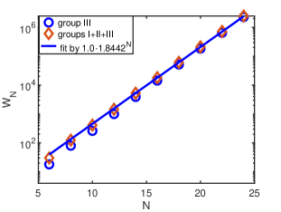
Figure 11: Numbers of states with all mobile spins vs the number of spins compared to the analytical fit $1.0\cdot 1.8442^{N}$

Appendix C Imbalance as a measure of system dynamic properties

Here we consider the definition of an infinite time imbalance in greater detail with special attention to its experimental determination. The imbalance is defined following the conditions of a typical experiment similarly to Ref. [2] (Eq. (39) in the main text). It is determined by the system evolution from some initial product state $|a>$, characterized by fixed projections of spins $\pm 1/2$ to the $z$ axis ($t=0$). The system evolution can be expressed in terms of average spin projections $<S_{k}^{z}(t)>$ at time $t$. The extraction of the infinite time limit for $<S_{k}^{z}(t)>$ is not straightforward using the experimental data available at a finite time only. Yet it can be estimated reasonably well as described below.

According to our observations imbalance converges to its infinite time limit quite fast for the initial state belonging to the groups I or II with delocalized eigenstates. For the family of initial states belonging to the group II, shown in Fig. 12.a, imbalances approach its infinite time limit during the time of order of few inverse spin hopping amplitudes $\Delta^{-1}$ Eq. (1). The convergence gets better with increasing the number of spins as illustrated in Fig. 12.a,.

For the localized state considered in Fig. 12.b, originated from the group III state, shown in the graph, the oscillations of imbalance around its infinite time limit are very strong. However, one can estimate the infinite time limit of imbalance using time averaged imbalance defined as

$$I_{av}(t)=\frac{\int_{0}^{t}I(\tau)d\tau}{t}.$$ (75)

According to Fig. 12.b the time averaged imbalance $I_{av}(t)$ converges to its infinite time limit after the time around few inverse hopping amplitudes $\Delta^{-1}$ similarly to Fig. 12.a. Thus the infinite time limit of imbalance can be determined experimentally and compared with the predictions of theory. One should notice that this definition can be not applicable in marginal situations of very slow dynamics emerging for instance for unlikely realized states of anomalously high or low energy [76].

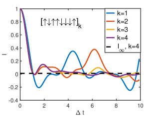
(a)

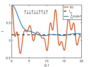
(b)

Figure 12: (a) Convergence of the imbalances for the family of states belonging to the group II to the infinite time limit. (b) Convergence of the time averaged imbalance to its infinite time limit for the localized state belonging to the group III. The initial product states are shown within the graphs in the inverted representation.

Eq. (39) determines the imbalance measured in Ref. [2] and we use it here for a characterization of different groups of states. The Hamming distances reported in Ref. [1] can be expressed as

$$HD(t)=1-\frac{4}{N}\sum_{k=1}^{N}<S_{k}^{z}(t)><S_{k}^{z}(0)>.$$ (76)

In a thermodynamic limit of $N\rightarrow\infty$ one can set $<S^{z}>=0$ in the definition of imbalance (Eq. (39) in the main text). Then two definitions becomes equivalent, since $HD(t)+I(t)=1$. However, we prefer to use Eq. (39) or its generalizations above since they are less sensitive to finite size effects due to the subtraction of the finite size expectation values for average spin projections.

References

- Guo et al. [2020] Qiujiang Guo, Chen Cheng, Hekang Li, Shibo Xu, Pengfei Zhang, Zhen Wang, Chao Song, Wuxin Liu, Wenhui Ren, Hang Dong, Rubem Mondaini, and H. Wang, “Stark many-body localization on a superconducting quantum processor,” (2020), arXiv:2011.13895 [quant-ph] .
- Morong et al. [2021] W. Morong, F. Liu, P. Becker, K. S. Collins, L. Feng, A. Kyprianidis, G. Pagano, T. You, A. V. Gorshkov, and C. Monroe, “Observation of Stark many-body localization without disorder,” (2021), arXiv:2102.07250 [quant-ph] .
- Deutsch [1991] J. M. Deutsch, “Quantum statistical mechanics in a closed system,” Phys. Rev. A 43, 2046–2049 (1991).
- Srednicki [1994] Mark Srednicki, “Chaos and quantum thermalization,” Phys. Rev. E 50, 888–901 (1994).
- Yao et al. [2016] N. Y. Yao, C. R. Laumann, J. I. Cirac, M. D. Lukin, and J. E. Moore, “Quasi-many-body localization in translation-invariant systems,” Phys. Rev. Lett. 117, 240601 (2016).
- Pekker et al. [2014] David Pekker, Gil Refael, Ehud Altman, Eugene Demler, and Vadim Oganesyan, “Hilbert-glass transition: New universality of temperature-tuned many-body dynamical quantum criticality,” Phys. Rev. X 4, 011052 (2014).
- Bahri et al. [2015] Yasaman Bahri, Ronen Vosk, Ehud Altman, and Ashvin Vishwanath, “Localization and topology protected quantum coherence at the edge of hot matter,” Nature Communications 6, 7341 (2015).
- Chandran et al. [2014] Anushya Chandran, Vedika Khemani, C. R. Laumann, and S. L. Sondhi, “Many-body localization and symmetry-protected topological order,” Phys. Rev. B 89, 144201 (2014).
- Gornyi et al. [2005] I. V. Gornyi, A. D. Mirlin, and D. G. Polyakov, “Interacting electrons in disordered wires: Anderson localization and low- transport,” Phys. Rev. Lett. 95, 206603 (2005).
- Basko et al. [2006] D.M. Basko, I.L. Aleiner, and B.L. Altshuler, “Metal-insulator transition in a weakly interacting many-electron system with localized single-particle states,” Annals of Physics 321, 1126 – 1205 (2006).
- Oganesyan and Huse [2007] Vadim Oganesyan and David A. Huse, “Localization of interacting fermions at high temperature,” Phys. Rev. B 75, 155111 (2007).
- Imbrie [2016] John Z. Imbrie, “On many-body localization for quantum spin chains,” Journal of Statistical Physics 163, 998–1048 (2016).
- Anderson [1958] P. W. Anderson, “Absence of diffusion in certain random lattices,” Phys. Rev. 109, 1492–1505 (1958).
- Fleishman and Anderson [1980] L. Fleishman and P. W. Anderson, “Interactions and the anderson transition,” Phys. Rev. B 21, 2366–2377 (1980).
- Kagan and Maksirnov [1984] Yu. Kagan and L. A. Maksirnov, “Localization in a system of interacting particles diffusing in a regular crystal,” Zh. Eksp. Teor. Fiz. 87, 348 (1984), [Sov. Phys. - JETP 60, 201 (1984)].
- Mikheev et al. [1983] V.A. Mikheev, V.A. Maidanov, and N.P. Mikhin, “Localization and quantum diffusion of He3 atoms stimulated by phonons in He4 crystals,” Solid State Communications 48, 361–364 (1983).
- Kagan and Maksirnov [1985] Yu. Kagan and L. A. Maksirnov, “Effect of interparticle interaction on localization in a nonideal crystal with a narrow band,” Zh. Eksp. Teor. Fiz. 88, 992 (1985), [Sov. Phys. - JETP 61, 583 (1985)].
- Burin et al. [1990] A. L. Burin, K. N. Kontor, and L. A. Maksimov, “Localization and delocalization in the paramagnetic phase of the transverse ising model,” Theoretical and Mathematical Physics 85, 1223–1230 (1990).
- Logan and Wolynes [1983] D.E. Logan and P. G. Wolynes, J. Chem. Phys. 78, 3907 (1983).
- Leitner and Wolynes [1997] David M. Leitner and Peter G. Wolynes, “Quantization of the stochastic pump model of arnold diffusion,” Phys. Rev. Lett. 79, 55–58 (1997).
- Georgeot and Shepelyansky [1998] B. Georgeot and D. L. Shepelyansky, “Integrability and quantum chaos in spin glass shards,” Phys. Rev. Lett. 81, 5129–5132 (1998).
- Carleo et al. [2012] Giuseppe Carleo, Federico Becca, Marco Schiró, and Michele Fabrizio, “Localization and glassy dynamics of many-body quantum systems,” Scientific Reports 2, 243 (2012).
- De Roeck and Huveneers [2014] Wojciech De Roeck and Fran çois Huveneers, “Scenario for delocalization in translation-invariant systems,” Phys. Rev. B 90, 165137 (2014).
- Schiulaz et al. [2015] Mauro Schiulaz, Alessandro Silva, and Markus Müller, “Dynamics in many-body localized quantum systems without disorder,” Phys. Rev. B 91, 184202 (2015).
- Papic et al. [2015] Z. Papic, E. Miles Stoudenmire, and Dmitry A. Abanin, “Many-body localization in disorder-free systems: The importance of finite-size constraints,” Annals of Physics 362, 714–725 (2015).
- Michailidis et al. [2018] Alexios A. Michailidis, Marko Žnidarič, Mariya Medvedyeva, Dmitry A. Abanin, Toma ž Prosen, and Z. Papić, “Slow dynamics in translation-invariant quantum lattice models,” Phys. Rev. B 97, 104307 (2018).
- Brenes et al. [2018] Marlon Brenes, Marcello Dalmonte, Markus Heyl, and Antonello Scardicchio, “Many-body localization dynamics from gauge invariance,” Phys. Rev. Lett. 120, 030601 (2018).
- Serbyn et al. [2021] Maksym Serbyn, Dmitry A. Abanin, and Zlatko Papić, “Quantum many-body scars and weak breaking of ergodicity,” Nature Physics 17, 675–685 (2021).
- Smith et al. [2017a] A. Smith, J. Knolle, D. L. Kovrizhin, and R. Moessner, “Disorder-free localization,” Phys. Rev. Lett. 118, 266601 (2017a).
- Smith et al. [2017b] A. Smith, J. Knolle, R. Moessner, and D. L. Kovrizhin, “Absence of ergodicity without quenched disorder: From quantum disentangled liquids to many-body localization,” Phys. Rev. Lett. 119, 176601 (2017b).
- van Nieuwenburg et al. [2019] Evert van Nieuwenburg, Yuval Baum, and Gil Refael, “From bloch oscillations to many-body localization in clean interacting systems,” Proceedings of the National Academy of Sciences 116, 9269–9274 (2019), https://www.pnas.org/content/116/19/9269.full.pdf .
- Schulz et al. [2019] M. Schulz, C. A. Hooley, R. Moessner, and F. Pollmann, “Stark many-body localization,” Phys. Rev. Lett. 122, 040606 (2019).
- Guardado-Sanchez et al. [2020] Elmer Guardado-Sanchez, Alan Morningstar, Benjamin M. Spar, Peter T. Brown, David A. Huse, and Waseem S. Bakr, “Subdiffusion and heat transport in a tilted two-dimensional fermi-hubbard system,” Phys. Rev. X 10, 011042 (2020).
- Smith et al. [2018] Adam Smith, Johannes Knolle, Roderich Moessner, and Dmitry L. Kovrizhin, “Dynamical localization in lattice gauge theories,” Phys. Rev. B 97, 245137 (2018).
- Sala et al. [2020] Pablo Sala, Tibor Rakovszky, Ruben Verresen, Michael Knap, and Frank Pollmann, “Ergodicity breaking arising from Hilbert space fragmentation in dipole-conserving hamiltonians,” Phys. Rev. X 10, 011047 (2020).
- Moudgalya et al. [2020a] Sanjay Moudgalya, B. Andrei Bernevig, and Nicolas Regnault, “Quantum many-body scars in a Landau level on a thin torus,” Phys. Rev. B 102, 195150 (2020a).
- Moudgalya et al. [2020b] Sanjay Moudgalya, Abhinav Prem, Rahul Nandkishore, Nicolas Regnault, and B. Andrei Bernevig, “Thermalization and its absence within Krylov subspaces of a constrained Hamiltonian,” (WORLD SCIENTIFIC, 2020) pp. 147–209, 0.
- Rakovszky et al. [2020] Tibor Rakovszky, Pablo Sala, Ruben Verresen, Michael Knap, and Frank Pollmann, “Statistical localization: From strong fragmentation to strong edge modes,” Phys. Rev. B 101, 125126 (2020).
- Khemani et al. [2020] Vedika Khemani, Michael Hermele, and Rahul Nandkishore, “Localization from Hilbert space shattering: From theory to physical realizations,” Phys. Rev. B 101, 174204 (2020).
- Morningstar et al. [2020] Alan Morningstar, Vedika Khemani, and David A. Huse, “Kinetically constrained freezing transition in a dipole-conserving system,” Phys. Rev. B 101, 214205 (2020).
- Herviou et al. [2021] Loïc Herviou, Jens H. Bardarson, and Nicolas Regnault, “Many-body localization in a fragmented Hilbert space,” Phys. Rev. B 103, 134207 (2021).
- Richter and Pal [2021] Jonas Richter and Arijeet Pal, “Anomalous hydrodynamics in a class of scarred frustration-free hamiltonians,” (2021), arXiv:2107.13612 [cond-mat.stat-mech] .
- Feldmeier et al. [2020] Johannes Feldmeier, Pablo Sala, Giuseppe De Tomasi, Frank Pollmann, and Michael Knap, “Anomalous diffusion in dipole- and higher-moment-conserving systems,” Phys. Rev. Lett. 125, 245303 (2020).
- García-Mata and Shepelyansky [2009] I. García-Mata and D. L. Shepelyansky, “Nonlinear delocalization on disordered stark ladder,” The European Physical Journal B 71, 121–124 (2009).
- Feldmeier and Knap [2021] Johannes Feldmeier and Michael Knap, “Critically slow operator dynamics in constrained many-body systems,” Phys. Rev. Lett. 127, 235301 (2021).
- Doggen et al. [2021] Elmer V. H. Doggen, Igor V. Gornyi, and Dmitry G. Polyakov, “Stark many-body localization: Evidence for Hilbert-space shattering,” Phys. Rev. B 103, L100202 (2021).
- Chanda et al. [2020] Titas Chanda, Ruixiao Yao, and Jakub Zakrzewski, “Coexistence of localized and extended phases: Many-body localization in a harmonic trap,” Phys. Rev. Research 2, 032039(R) (2020).
- Bergholtz and Karlhede [2005] Emil J. Bergholtz and Anders Karlhede, “Half-filled lowest Landau level on a thin torus,” Phys. Rev. Lett. 94, 026802 (2005).
- Seidel et al. [2005] Alexander Seidel, Henry Fu, Dung-Hai Lee, Jon Magne Leinaas, and Joel Moore, “Incompressible quantum liquids and new conservation laws,” Phys. Rev. Lett. 95, 266405 (2005).
- Wang et al. [2012] Zheng-Yuan Wang, Shintaro Takayoshi, and Masaaki Nakamura, “Spin-chain description of fractional quantum Hall states in the jain series,” Phys. Rev. B 86, 155104 (2012).
- Scherg et al. [2021] Sebastian Scherg, Thomas Kohlert, Pablo Sala, Frank Pollmann, Bharath Hebbe Madhusudhana, Immanuel Bloch, and Monika Aidelsburger, “Observing non-ergodicity due to kinetic constraints in tilted Fermi-Hubbard chains,” Nature Communications 12, 4490 (2021).
- Turner et al. [2018] C. J. Turner, A. A. Michailidis, D. A. Abanin, M. Serbyn, and Z. Papić, “Weak ergodicity breaking from quantum many-body scars,” Nature Physics 14, 745–749 (2018).
- Pai et al. [2019] Shriya Pai, Michael Pretko, and Rahul M. Nandkishore, “Localization in fractonic random circuits,” Phys. Rev. X 9, 021003 (2019).
- Schreiber et al. [2015] Michael Schreiber, Sean S. Hodgman, Pranjal Bordia, Henrik P. Lüschen, Mark H. Fischer, Ronen Vosk, Ehud Altman, Ulrich Schneider, and Immanuel Bloch, “Observation of many-body localization of interacting fermions in a quasirandom optical lattice,” Science 349, 842–845 (2015).
- Strichartz [1987] Robert S Strichartz, “The Campbell-Baker-Hausdorff-Dynkin formula and solutions of differential equations,” Journal of Functional Analysis 72, 320–345 (1987).
- Achilles and Bonfiglioli [2012] Rüdiger Achilles and Andrea Bonfiglioli, “The early proofs of the theorem of Campbell, Baker, Hausdorff, and Dynkin,” Archive for History of Exact Sciences 66, 295–358 (2012).
- Burin [2015a] Alexander L. Burin, “Localization in a random xy model with long-range interactions: Intermediate case between single-particle and many-body problems,” Phys. Rev. B 92, 104428 (2015a).
- Maksymov and Burin [2019] Andrii O. Maksymov and Alexander L. Burin, “Many-body localization in spin chains with the long-range transverse interactions: scaling of critical disorder with the system size,” arXiv:1905.02286 (2019).
- Wybo et al. [2021] Elisabeth Wybo, Michael Knap, and Frank Pollmann, “Dynamics of negativity of a Wannier-Stark many-body localized system coupled to a bath,” (2021), arXiv:2110.07384 [quant-ph] .
- Taylor et al. [2020] S. R. Taylor, M. Schulz, F. Pollmann, and R. Moessner, “Experimental probes of stark many-body localization,” Phys. Rev. B 102, 054206 (2020).
- Jordan and Wigner [1928] P. Jordan and E. Wigner, “Uber das Paulische aquivalenzverbot,” Zeitschricht für Physik 47, 42 (1928).
- Schrieffer and Wolff [1966] J. R. Schrieffer and P. A. Wolff, “Relation between the Anderson and Kondo Hamiltonians,” Phys. Rev. 149, 491–492 (1966).
- Biagi et al. [2020] Stefano Biagi, Andrea Bonfiglioli, and Marco Matone, “On the baker-campbell-hausdorff theorem: non-convergence and prolongation issues,” Linear and Multilinear Algebra 68, 1310–1328 (2020), https://doi.org/10.1080/03081087.2018.1540534 .
- Huse et al. [2015] David A. Huse, Rahul Nandkishore, Francesca Pietracaprina, Valentina Ros, and Antonello Scardicchio, “Localized systems coupled to small baths: From anderson to zeno,” Phys. Rev. B 92, 014203 (2015).
- L schen et al. [2016] H. P. L schen, P. Bordia, S. S. Hodgman, M. Schreiber, S. Sarkar, A. J. Daley, M. H. Fischer, E. Altman, I. Bloch, and U. Schneider, “Signatures of many-body localization in a controlled open quantum system,” arXiv:1610.01613 (2016).
- Berezinskii and Gor’kov [1979] V.L. Berezinskii and L.P. Gor’kov, “On the theory of electrons localized in the field of defects,” Zh. Eksp. Teor. Fiz. 77, 2498 (1979), [Sov. Phys. - JETP 50, 1209 (1979)].
- Kudo and Deguchi [2004] Kazue Kudo and Tetsuo Deguchi, “Level statistics of spin chains with a random magnetic field,” Phys. Rev. B 69, 132404 (2004).
- Burin et al. [1998a] Alexander L. Burin, Douglas Natelson, Douglas D. Osheroff, and Yuri Kagan, “Interactions between tunneling defects in amorphous solids,” in Tunneling Systems in Amorphous and Crystalline Solids, edited by Pablo Esquinazi (Springer Berlin Heidelberg, Berlin, Heidelberg, 1998) pp. 223–315.
- Burin et al. [1998b] A. L. Burin, Yu. Kagan, L. A. Maksimov, and I. Ya. Polishchuk, “Dephasing rate in dielectric glasses at ultralow temperatures,” Phys. Rev. Lett. 80, 2945–2948 (1998b).
- Burin [2005] A. L. Burin, “Energy delocalization in strongly disordered systems induced by the long-range many-body interaction,” arXiv:cond-mat/0611387 (2005).
- Serbyn et al. [2014] M. Serbyn, M. Knap, S. Gopalakrishnan, Z. Papic, N. Y. Yao, C. R. Laumann, D. A. Abanin, M. D. Lukin, and E. A. Demler, “Interferometric probes of many-body localization,” Phys. Rev. Lett. 113, 147204 (2014).
- Burin [2015b] Alexander L. Burin, “Many-body delocalization in a strongly disordered system with long-range interactions: Finite-size scaling,” Phys. Rev. B 91, 094202 (2015b).
- Wang et al. [2021] Yong-Yi Wang, Zheng-Hang Sun, and Heng Fan, “Stark many-body localization transitions in superconducting circuits,” Phys. Rev. B 104, 205122 (2021).
- Huveneers [2017] François Huveneers, “Classical and quantum systems: transport due to rare events,” Annalen der Physik 529, 1600384 (2017).
- Lang et al. [2022] Haifeng Lang, Philipp Hauke, Johannes Knolle, Fabian Grusdt, and Jad C. Halimeh, “Disorder-free localization with Stark gauge protection,” arXiv:cond-mat/2203.01338 (2022), 10.48550/ARXIV.2203.01338.
- Maksymov et al. [2017] Andrii O. Maksymov, Noah Rahman, Eliot Kapit, and Alexander L. Burin, “Comment on “many-body localization in ising models with random long-range interactions”,” Physical Review A 96, 057601 (2017).