Keypoint-Based Bimanual Shaping of Deformable Linear Objects under Environmental Constraints using Hierarchical Action Planning

Abstract

This paper addresses the problem of contact-based manipulation of deformable linear objects (DLOs) towards desired shapes with a dual-arm robotic system. To alleviate the burden of high-dimensional continuous state-action spaces, we model the DLO as a kinematic multibody system via our proposed keypoint detection network. This new perception network is trained on a synthetic labeled image dataset and transferred to real manipulation scenarios without conducting any manual annotations. Our goal-conditioned policy can efficiently learn to rearrange the configuration of the DLO based on the detected keypoints. The proposed hierarchical action framework tackles the manipulation problem in a coarse-to-fine manner (with high-level task planning and low-level motion control) by leveraging on two action primitives. The identification of deformation properties is avoided since the algorithm replans its motion after each bimanual execution. The conducted experimental results reveal that our method achieves high performance in state representation of the DLO, and is robust to uncertain environmental constraints.

I INTRODUCTION

Deformable object manipulation has many promising applications in growing fields, such as flexible cable arrangement [1], clothes folding [2], and surgical robots [3]. Among them, manipulation of deformable linear objects (DLOs) attracts much attraction due to its relevance in several manufacturing industries [4], such as wiring harness and knot tying [5].

Although great progress has been recently achieved in deformable object manipulation (e.g. [6, 7, 8]), shaping DLOs with environmental contacts remains an open problem. Compared with rigid objects, this problem is much more challenging due to the complex physical dynamics of infinite degree-of-freedom DLOs. Our strategy is that instead of analytic physical dynamics, the DLO modeling is simplified to a kinematic multibody featured by several keypoints. The assumptions of our strategy are 1) the keypoint representation is sufficient for the contact-based shape matching problem, and 2) the shape error incurred by the modeling simplicity can be compensated for by coarse-to-fine manipulation. This paper aims to develop a complete algorithm (including perception and planning) to tackle the task of contact-based shaping of DLOs with bimanual manipulation.

Many researchers have worked on the representation of DLOs in vision [9]. Angles [10] and curvatures [11] are intuitive hard-coded descriptors for shape feedback, whose generalization is poor. [1, 8] develop Fourier-based descriptor; however, they require high computation cost during online perception. Data-driven based shape analysis has gained popularity in feature extraction [12]. [13] employs the Gaussian Mixture Model for its physics simulation engine, assuming the physical model of the deformable objects is known. [14] proposes an Encode-Manipulate-Decode network for cloth manipulation. However, it needs tremendous data collection and the latent vector is not semantic. Since real data is expensive to collect, learning on synthetic datasets and transferring to physical situations is an alternative solution [15]. [16] simulates 2D fabric smoothing on a mesh grid connected by various springs. [17] forms a braid of rope through twisting cylindrical meshes; this work needs a sphere mesh on one end to break out the symmetry. [18] generates images with a random b-spline curve with six control points; however, it still needs a real dataset for perception finetuning.

Robotic manipulation of deformable objects has been studied with various formulations and assumptions, including model-based and model-free approaches. With the pregrasping hypothesis, [1, 19] consider the deforming task as shape servoing and approximate the local deformation model with a linear Jacobian matrix, while the global convergence is not guaranteed. Formulating the task as a multi-step pick-and-place manipulation problem, [17, 18] conduct the tasks with single-arm policy while real data collection is required for sim-to-real transferring or human visual demonstration. [20] assembles DLOs for specified fixtures with dual robots, yet contacts are not taken into consideration. Task and motion planning (TAMP) is a solution to tackle this multi-step decision-making task [21] through factorizing [22] the planning process into discrete symbolic reasoning and continuous motion generation [23]. However, a majority of TAMP algorithms assume rigid objects, whose predictable dynamics are not available in deformable objects, let alone under contact constraints.

[24] exploits environmental contacts for manipulation of DLOs, which is achieved with some customized mechanical grippers and the assumption of pregrasping. We advance the achievement to manipulating DLOs from arbitrary configurations to the desired goal states under environmental constraints. The shape of the DLO is characterized with a sequence of ordered keypoints, an approach that narrows the state-action search space for bimanual manipulation. To deal with the complex contact configurations, a coarse-to-fine planning framework with two defined action primitives is derived. The original contributions of this work are as follows:

• A novel data-driven perception approach for DLOs whose network is trained on a synthetic dataset.

• A hierarchical action planning framework for shaping DLOs under environmental constraints in a coarse-to-fine manner.

• Experimental results to validate our solution for contact-based DLOs bimanual manipulation in real environments.

The remainder of this paper is organized as follows. Sec. II states the task’s formulation. Sec. III explains the perception. Sec. IV reports the planning framework. Sec. V reports the results and Sec. VI gives the conclusions.

II PROBLEM FORMULATION

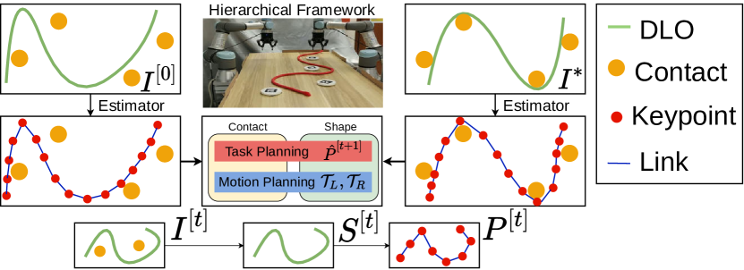
Figure 1: Overview of the keypoint-based bimanual manipulation framework for shaping DLOs with contacts. Given the goal $I^{*}$, the DLO manipulation is formulated as a goal-directed task from the initial configuration $I^{[0]}$. At each time step $t$, the perception detects the sequential keypoints $P^{[t]}$ corresponding to the state of the DLO $S^{[t]}$ extracted from the visual observation $I^{[t]}$. The hierarchical control framework takes the current $P^{[t]}$ and the goal $P^{*}$ keypoints as input and outputs the action plan ($\mathcal{T}_{L},\mathcal{T}_{R}$). The whole algorithm replans based on the new observation after the execution of the robots. The scheme iterates until reaching the desired goal.

The architecture of our vision-based manipulation system is depicted in Fig. 1. Given a goal observation $I^{*}$, our task is to manipulate the DLO with an initial configuration $I^{[0]}$ to match it. Assuming the DLO has an obvious color contrast with the background, we segment the state of the DLO $S^{[t]}$ from a raw image $I^{[t]}$ with a color filter. To simplify the problem, we consider circular contacts with known size $C=\{c_{1},\cdots,c_{k},\cdots,c_{q}\}$ in the observation $I^{[t]}$.

Formulating deformable object manipulation as a multi-step decision-making process, our aim is to obtain an action plan $\mathcal{A}=(A^{[1]},\cdots,A^{[t]},\cdots,A^{[H]})$ within $H$ steps, such that the last state $S^{[H+1]}$ (with the transition function $S^{[H+1]}=A^{[H]}\times S^{[H]}$) reaches the goal state $S^{*}$. To apply TAMP framework for this challenging task, we make some modifications versus perception and planning. The state $S^{[t]}$ of the DLO is depicted as $S^{[t]}=\{s_{1}^{[t]},\cdots,s_{i}^{[t]},\cdots,s_{n}^{[t]}\}$. Based on the kinematic multibody model [25], we describe the DLO $S^{[t]}$ as a list of sequential keypoints $P^{[t]}=\{p_{1}^{[t]},\cdots,p_{j}^{[t]},\cdots,p_{m}^{[t]}\}$ ($m\ll n$) since it allows us to 1) narrow down the search space from high-dimensional state to low-dimensional latent space, and 2) obtain a compact feedback vector for semantic bimanual manipulation. Note that the end of the DLO closer to the left robot is denoted as the first keypoint in the perception. Based on the description, our hierarchical control framework combines high-level task planning and low-level motion control. Taking $P^{[t]}$ and $P^{*}$ as input, the high-level model designs the sub-goals $\hat{P}^{[t+1]}$, while low-level model plans the local motion $A^{[t]}$ to achieve $\hat{P}^{[t+1]}$. Note that $\hat{P}^{[t+1]}$ is the designed sub-goal and is different from the detected keypoints $P^{[t+1]}$ at time step $t+1$. We choose bimanual manipulation in a tabletop environment instead of a single-arm to 1) constraint the unpredictable displacement of the DLO, and 2) enrich the diversity of the action. In this case, each plan $A^{[t]}$ is defined as $A^{[t]}=[\mathcal{T}^{[t]}_{L}\ \mathcal{T}^{[t]}_{R}]$, where $\mathcal{T}^{[t]}_{L}$ and $\mathcal{T}^{[t]}_{R}$ are the actions of the left and right arm, respectively, including motion, grasping, and releasing.

III Perception

Our perception takes the visual binary image $S^{[t]}$ as input and outputs the corresponding keypoints $P^{[t]}$. To avoid time-consuming real-world data collection for training, we render an annotated synthetic image dataset for supervised learning (Sec. III-A) and finetune the output of the network through the geometric constraints (Sec. III-B).

III-A Synthetic Dataset Generation

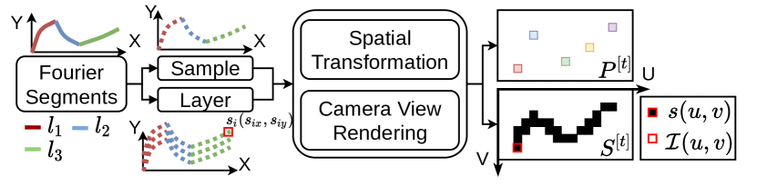
Figure 2: Data generation of labeled synthetic DLOs. Base on the Fourier series, we generate multiple curve segments and concatenate them end-to-end. This raw data undergoes sampling and stacking for keypoint labels and image input, respectively. After the spatial transformation for data augmentation, we simulate image rendering based on the camera acquisition principle.

In this section, we simulate DLOs to facilitate the keypoint detection $P^{[t]}$ from the binary image $S^{[t]}$, as illustrated in Fig. 2. Geometrically, a DLO refers to an object whose length is much larger than the diameter of its cross-section. Thus, we mathematically describe it as a continuous curve. Taking the deformation of DLOs into consideration, our model utilizes several 2D curve segments based on the Fourier series [8] to depict the local shape of DLOs $(l_{1},l_{2},\cdots)$, where each curve segment $l$ is described along the X-axis:

$$y=f(x)=\frac{a_{0}}{2}+\sum_{n=1}^{N}\left[a_{n}\cos(n\omega x)+b_{n}\sin(n\omega x)\right]$$ (1)

where $a_{0}$ is the bias of the Fourier descriptor at zero frequency and $N$ is the number of harmonics under consideration. The coefficients of the n-th harmonic $a_{n},b_{n}$ are defined as $a_{n}=\frac{2}{T}\int_{t_{0}}^{t_{0}+T}f(t)\cos(n\omega t)dt$ and $b_{n}=\frac{2}{T}\int_{t_{0}}^{t_{0}+T}f(t)\sin(n\omega t)dt$, respectively, where $\omega$ denotes the frequency. Note that the discrete points of the curve $l$ are in order along the X-axis with this definition. Each DLO $L$ consists of several end-to-end connected Fourier series-based segments $L=(l_{1},l_{2},\cdots)$ and the point of it is represented as $s_{i}=(s_{ix},s_{iy})$. Next, we simulate the raw input $S^{[t]}$ and our desired keypoints $P^{[t]}$, respectively. We denote $m$ keypoints from $S^{[t]}$ in a coarse-to-fine manner. Initially, $m$ candidates are sampled uniformly according to Euclidean distance. Since the points with high curvature describe the contour of the DLO, we also desire those as keypoints. The curvature of a point $s_{i}$ is defined as:

$$\alpha_{i}=\left<f_{-}^{\prime}(s_{i}),f_{+}^{\prime}(s_{i})\right>$$ (2)

where $f_{-}^{\prime}(s_{i})=\vec{s}_{i}-\vec{s}_{i-1}$ and $f_{+}^{\prime}(s_{i})=\vec{s}_{i+1}-\vec{s}_{i}$. Here, $\left<\vec{a},\vec{b}\right>$ denotes the function about computing the angle between two vectors $(\vec{a},\vec{b})$. According to this definition, we substitute the points whose curvatures are larger than a threshold $\tau_{u}$ for their corresponding nearest uniform candidates, enabling the number of the keypoints keeping a constant $m$. For $S^{[t]}$, we stack the curve $L$ along Y-axis to simulate the cross-section of the DLO. After these steps, both the sampled keypoints and the stacked layers enter into spatial transformation for data augmentation and camera view rendering for image processing. Spatial transformation, including translation and rotation, is significant for balancing the distribution of samples. Camera view rendering consists of resizing the curve into the region of interest and reorder of the points into an image format. Since we adopt a binary image $S^{[t]}$ to represent the DLO, the pixel at $S(u,v)$ is positive if any point locates within its surroundings:

$$S(u,v)=\left\{\begin{aligned} 1,\quad&\exists s_{i}\in\mathcal{I}(u,v)\\ 0,\quad&otherwise\end{aligned}\right.$$ (3)

where $s_{i}\in\mathcal{I}(u,v)\Longleftrightarrow\{w_{u}<s_{ix}<w_{u+1}\}\cap\{h_{v}<s_{iy}<h_{v+1}\}$, $u$ and $v$ are the horizontal and vertical position of the pixel in the image, respectively. For the labeled keypoints, we transform them from Cartesian frame to image frame, represented as $p_{j}(u_{j},v_{j})$ in sequence.

With this generation pipeline, we obtain binary images describing the shape of DLOs and their corresponding annotated sequential keypoints.

III-B Keypoint Detection

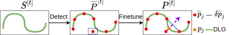
Figure 3: Illustration of the geometric finetuning. The point locating on the background area is revised along the direction vertical to its tangent.

To detect the keypoints from the visual image $S^{[t]}$, we design a network to predict the keypoints of DLOs. More details about the network structure and the training process are discussed in Sec V.

While the network is generalizable across different shapes of DLOs, errors are still unavoidable. As illustrated in Fig. 3, some outputs visually locate on the area of the background, which conflicts with the prior knowledge that the keypoints locate within the DLO. Hence, we consider this geometric constraint finetuning. For an output $\overline{p}_{j}=(\overline{u}_{j},\overline{v}_{j})$ that fails, namely $S^{[t]}(\overline{u}_{j},\overline{v}_{j})=0$, we utilize the adjacent pixels $(\overline{p}_{j-1},\overline{p}_{j+1})$ to correct it, which is divided into two cases: (1) the ends are adjusted to the nearest pixels in the area of DLO and (2) the intermediate keypoints are revised through searching along the direction vertical to its tangent space $\delta\overline{p}_{j}$:

$$find\quad s_{i}(u_{i},v_{i})$$ (4)

$$\begin{array}[]{r@{\quad}r@{}l@{\quad}l}s.t.&S^{[t]}(u_{i},v_{i})=1\\ &\overrightarrow{s_{i}\overline{p}_{j}}\cdot\delta\overline{p}_{j}=0\\ \end{array}$$

where its tangent space $\delta\overline{p}_{j}$ is defined as $\delta\overline{p}_{j}=\vec{\overline{p}}_{j+1}-\vec{\overline{p}}_{j-1}$. Notably, we denote $P^{[t]}$ as the finetuning result of the raw output $\overline{P}^{[t]}$.

IV Hierarchical Action Planning

We propose a hierarchical action planning framework interleaving high-level task planning, where a sub-goal $\hat{P}^{[t+1]}$ is designed given the detected keypoints ($P^{[t]}$,$P^{*}$), and low-level motion control, where a search-based action plan ($\mathcal{T}_{L}$,$\mathcal{T}_{R}$) is derived at each time step $t$. Specifically, the design task $\hat{P}^{[t+1]}$ investigates the interested keypoints specification (selection and placement) of dual arms respectively, whereas ($\mathcal{T}_{L}$,$\mathcal{T}_{R}$) is an action plan to manipulate the DLO to the detailed configuration. Under this framework, we define two multi-step action primitives, the contact primitive and the shape primitive to implement the task in a coarse-to-fine manner. The switch between them depends on the analysis of the contact constraints, as illustrated in Fig. 4. Sharing the same classical pick-and-place manipulation configuration between the primitives, we first detail the contact primitive (Sec. IV-A) and highlight the difference of the shape primitive (Sec. IV-B) afterward.

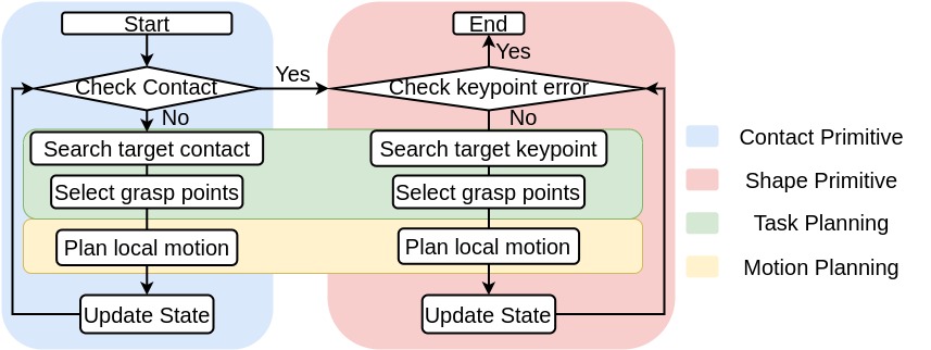
Figure 4: Flow chart depicting the conversion and details of the action primitives.

IV-A Contact Primitive

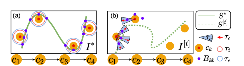
Figure 5: Graphical explanation of the contact primitive. (a) Based on the distance threshold $\tau_{i}$ and $\tau_{e}$, we acquire the benchmark $B_{k}$ in the goal state $S^{*}$ with respect to the contact $c_{k}$. (b) Based on the threshold $\tau_{c}$ and $\tau_{a}$, we search points that meet the conditions with respect to each benchmark $B_{kb}$.

while $c_{k}\neq\varnothing$ do

       $\mathcal{T}_{L},\mathcal{T}_{R}\leftarrow$ GraspPlan ($P^{[t]},C,c_{k},J$)

       if Reachable($c_{k},B^{\prime}_{k}$) then

             $\mathcal{T}_{R}\leftarrow\mathcal{T}_{R}\cup$ Motion($c_{k},\mathcal{B}^{\prime}_{k}$)

            

      else

             $\mathcal{T}_{L}\leftarrow\mathcal{T}_{L}\cup$ Motion($c_{k},\mathcal{B}^{\prime}_{k}$)

            

      $S^{[t+1]}\leftarrow$ System Dynamics $(\mathcal{T}_{L},\mathcal{T}_{R},S^{[t]})$

       $P^{[t+1]}\leftarrow$Update keypoints $(S^{[t+1]})$

       $c_{k}\leftarrow$ ContactSearch($P^{[t]},C,\mathcal{B}$)

      

Algorithm 1 ContactPrimitive($P^{[t]},P^{*},C,\mathcal{J},\mathcal{B},\mathcal{B}^{\prime}$)

Unlike the common robotic manipulation tasks, i.e., grasping, pushing, shape servoing, shaping DLOs under environmental constraints is a discrete-continuous mixed manipulation task, since contacts also provide external force for DLOs besides robots. With the state $S^{*}$ extracted from desired goal observation $I^{*}$, DLOs reach and stay in this goal configuration only if the contacts are constructed correctly. Hence, it is significant to construct the contacts first as coarse matching, denoted as contact primitive. The whole algorithm of this primitive is shown in Alg. 1.

Firstly, we analyze the role of contacts in shaping the DLO as $S^{*}$, as illustrated in Fig. 5(a). Each contact $c_{k}$ supports its adjacent elements of the DLO, constraining its mobility. Hence, our algorithm validates the contact construction according to these elements. Specifically, we denote a set of benchmarks $\mathcal{B}=\{B_{kb}|k=1,\cdots,q,b=1,2,3\}$ for contact evaluation, which three benchmarks $(B_{k1},B_{k2},B_{k3})$ are defined for a contact $c_{k}$. Among them, the benchmarks ($B_{k1},B_{k2}$) are obtained through constrained optimization:

$$B_{k1}=\arg\max_{s_{i}}||s_{i} -c_{k}||_{2},B_{k2}=\arg\max_{s_{i}}||s_{i}-B_{k1}||_{2}$$ (5)

$$s.t. \tau_{i}<||s_{i}-c_{k}||_{2}<\tau_{e}$$

where ($\tau_{i}$,$\tau_{e}$) is distance threshold of the search area. In addition, we also search for the nearest element $s^{*}_{i}$ of the goal shape $S^{*}$ to emphasize the support force from the contact $c_{k}$ to the DLO,

$$B_{k3}=\arg\min_{s_{i}}||s_{i}-c_{k}||_{2}$$ (6)

After the search, we re-order the benchmarks $B_{kb}\in\mathcal{B}$ along the sequential keypoints $P^{*}$. These benchmarks act as baselines to assess the contact construction. A benchmark $B_{kb}$ is satisfied if we find an element $s_{i}$ that fulfills two thresholds $\tau_{c}$ and $\tau_{a}$ (graphical explanation in Fig. 5(b)):

$$\begin{cases}||s_{i}-c_{k}||_{2}&<\tau_{c}\\ \left<\overrightarrow{c_{k}s_{i}},\overrightarrow{c_{k}B_{kb}}\right>&<\tau_{a}\end{cases}$$ (7)

For a contact $c_{k}$, we consider it as qualified only if all the benchmarks $\{B_{kb}|b=1,2,3\}$ are satisfied based on the metrics. According to the benchmark set $\mathcal{B}$, we search the target contact along the sequence of $k=2,\cdots,q,1$, meaning that the first contact on the end is skipped and placed in the last of the queue. This priority distribution avoids breaking out the constructed contacts on the end while manipulating the central part of the DLO. Note that this search paradigm stops once the target contact $c_{k}$ is acquired along the defined sequence.

Our low-level planner takes the target contact $c_{k}$ as input and output the motion of the dual-arm robot $(\mathcal{T}_{L},\mathcal{T}_{R})$ to achieve it. The benchmark set $\mathcal{B}$ also serves as the guidance for contact construction, whereas there exists a gap between the keypoints $P^{[t]}$ and $\mathcal{B}$. To link the benchmark $\mathcal{B}$ and the keypoints $P^{*}$, we pair them up with the nearest Euclidean distance, using a set $\mathcal{J}=\{J_{kb}|k=1,\cdots,q,b=1,2,3\}$ to mark the corresponding index:

$$J_{kb}=\arg\min_{i}||\vec{p}_{i}^{*}-\vec{B}_{kb}||_{2}$$ (8)

With the set $\mathcal{J}$, the search sequence of grasping points selection for individual robots is divided into two cases 1) starting from the ends to the middle for $c_{k}$ on the end and 2) starting from the middle to the ends for $c_{k}$ in the intermediate. This solution enables to limit the impacts caused by the manipulation on unrelated sections of the DLO. This search paradigm undertakes under the constraints of the system, including the operation range and the contact obstacles.

Next, we build on potential field [26] path planning to avoid the collision with the contacts, which provide a repulsion force to the robot. Specifically, we extend the benchmark set $\mathcal{B}$ to $\mathcal{B}^{\prime}$ with a threshold $\tau_{b}$:

$$B_{kb}^{\prime}=\vec{c}_{k}+\tau_{b}\cdot\overrightarrow{c_{k}B_{kb}}/||\vec{B}_{kb}-\vec{c}_{k}||_{2},$$ (9)

For the target contact $c_{k}$, we manipulate the DLO to the corresponding extended benchmark $\{B^{\prime}_{kb}|b=1,2,3\}$. During the action, dual arms are assigned as fixing for freedom constraints and moving for shaping, depending on the reachability analysis of the robot arm concerning $B^{\prime}_{k1}$. After that, the motion path is $B_{k3}$ to $B_{k_{1}}$ for left arm or $B_{k1}$ or $B_{k_{3}}$ for the right arm.

The 4-DOF pose on a table-top environment is defined as $\pi_{j}=\{\vec{\chi}_{j},\vec{\eta}_{j}\}$, where $\vec{\chi}_{j}$ and $\vec{\eta}_{j}$ are position and direction vectors of $3\times 1$. These two entities are defined by:

$$\vec{\chi}_{j}=B^{\prime}_{kb},\ \vec{\eta}_{j}\cdot\overrightarrow{c_{k}B^{\prime}_{kb}}=0$$ (10)

At last, we give a summary about the primitive. With the target contact $c_{k}$, we select the grasping points for dual arms. Next, we assign their roles and execute the motion. At last, the robots release the DLO, waiting for the re-planning.

IV-B Shape Primitive

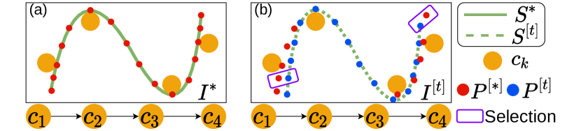
Figure 6: Graphical explanation of the shape primitive. (a) The desired goal guides the framework for shaping. (b) Based on the goal and the current state, we select the points of interest to reshape.

The goal of the shape primitive is to implement the finetuning after the contact construction. As illustrated in Fig. 6, our perception network correspondingly pairs up individual keypoints $p_{j}^{[t]}\in P^{[t]}$ and $p_{j}^{*}\in P^{*}$. Hence, the shape error $\Delta P$ between them is defined as:

$$\Delta P=\frac{1}{m}\sum_{j=1}^{m}||p^{[t]}_{j}-p^{*}_{j}||_{2}$$ (11)

This error serves as a guidance to improve the similarity. Intuitively, we select the keypoints $p_{j}$ whose difference between the current stage $P^{[t]}$ and the goal stage $P^{*}$ is comparatively large. Meanwhile, we also find the one in second-level for bimanual manipulation:

$$g\leftarrow\arg\max_{j}||p^{[t]}_{j}-p^{*}_{j}||_{2},g^{\prime}\leftarrow\arg\max_{j,j\neq g}||p^{[t]}_{j}-p^{*}_{j}||_{2}$$ (12)

We reorder $(g,g^{\prime})$ and reassign it to the dual-arm robot by

$$g_{L},g_{R}\leftarrow\min(g,g^{\prime}),\max(g,g^{\prime})$$ (13)

Similar to the contact primitive, we define the search paradigm under the system constraints as $g_{L}$ to $1$ for left arm and $g_{R}$ to $m$ for the right arm, respectively. Then, we define the target pose with respect to the g-th keypoint $p^{*}_{g}$:

$$\pi_{g}=\{\vec{p}_{g}^{*},\delta p^{*}_{g}\}$$ (14)

where $\delta p^{*}_{g}$ is tangent of $p^{*}_{g}$. This shape primitive iterates until the desired goal is reached.

V RESULTS

V-A Hardware Setup

As illustrated in Fig. 1, our bimanual experimental platform consists of two UR3 robotic manipulators, equipped with 2-fingered Robotiq grippers, respectively. To facilitate the bimanual manipulation, they face each other with an interval of $0.6m$. An Intel Realsense L515 camera is mounted to sense the top-down view of the manipulation space with a resolution of $1280\times 780$. The spatial transformation between the depth camera and dual-arms $(\mathbb{T}^{L},\mathbb{T}^{R})$ is calibrated through the markers. Each contact is a cylinder (radius=4cm,height=1cm), localized via ArUco markers. All contacts are glued on the table, keeping them stable during the whole manipulation process. The contacts are conventionally ordered according to the detected sequential keypoints $P^{*}$ concerning the goal shape of DLO $S^{*}$. Considering the physical limitations, the operation space of individual robots is constrained to a ring-shaped region.

V-B Perception

For perception in real environment, we utilize OpenCV [27] to segment the DLO $S^{[t]}$ from the raw observation $I^{[t]}$ with a morphological operation-based color filter, represented as a binary image. To balance the accuracy and efficiency, we resized $S^{[t]}$ to $128\times 64$ for the following processing.

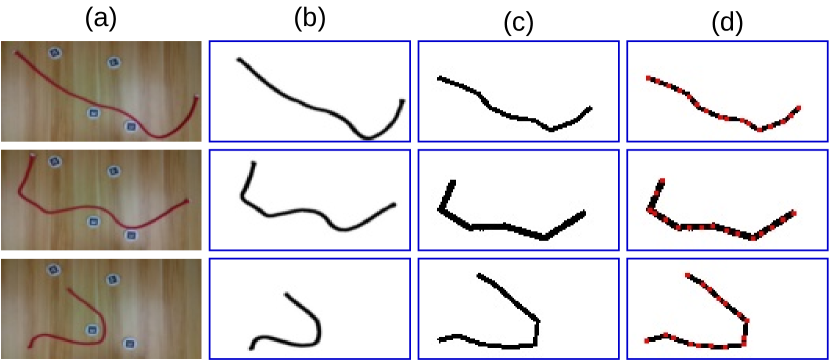
Figure 7: Visualizations of synthetic dataset and the comparison with the real collected data. (a) Visual observation. (b) Extracted state of the DLO by the color filter. (c) Rendered state of the DLO. (d) Rendered keypoints of the DLO.

In this section, we introduce the superiority of our synthetic-based feature extraction without any manual data collection and annotations. To reduce the gap between simulation and reality, the synthetic dataset needs to render the physics. We quantitatively and qualitatively evaluate the robustness and accuracy of the perception model.

Fig. 7 visualizes the synthetic dataset concerning the real data. Note that Fig. 7(a)-(b) is designed manually to act as references to have an intuitive comparison with the simulated Fig. 7(c)-(d). These graphical results validate the visual similarity with the real dataset. Our synthetic dataset includes 7040 labeled images in total, divided into a training dataset and testing dataset with a ratio of 10:1. Each sample is rendered as a binary image, containing a randomly generated curve and $m=16$ corresponding sorted keypoints in image coordinates. To improve the variation of the dataset, the geometry features of the DLO, including radius, length, and the number of segments, are randomly generated over a wide range.

Based on the synthetic dataset, we train our supervised keypoint detection network, whose architecture is shown in Fig. 8(a). As a fully convolution network [28], it only involves convolution layers with a similar structure to VGG [29]. In the last layer, we apply $1\times 1$ convolution to regress the dimension of the output as $2\times 16$, where each column represents the position $\overline{p}_{j}=(\overline{u}_{j},\overline{v}_{j})$ in the image frame. The training is optimized based on the smooth L1 loss function

$$\mathcal{L}_{1}(y,\hat{y})=\begin{cases}\frac{1}{2}(y-\hat{y})^{2}&\text{ for }|y-\hat{y}|\leq 1\\ |y-\hat{y}|-0.5&\text{ otherwise }\end{cases}$$ (15)

where $y$ and $\hat{y}$ denote the ground truth and the output of the training, respectively.

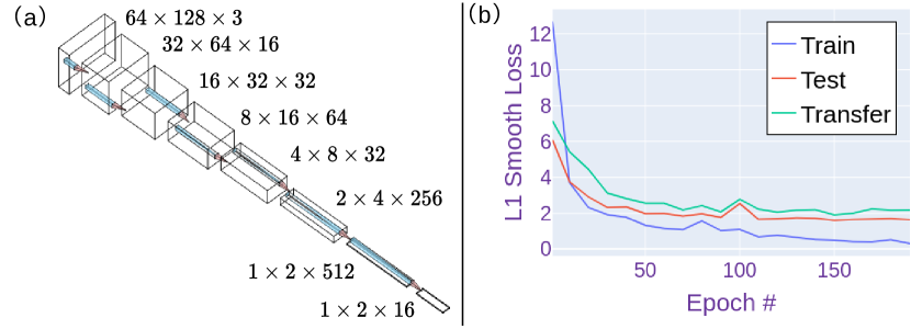
Figure 8: Details about the perception network. (a) Architecture of the FCN network. (b) Loss convergence of training, validation, testing, and transferring.

Fig. 8(b) shows the corresponding loss trend for training, testing, and transferring. Note that both training and testing are implemented with our synthetic dataset for efficient processing. In addition, the transfer loss is evaluated on the real data collection with manual annotation, which includes fifty samples. Note that this manual collection dataset is only for evaluation and is not used to train the network. The promising results reveal the advantages of our perception method: 1) our synthetic dataset holds a high similarity with the real data to avoid manual collection; 2) the keypoint detection network converges to minimize the detection error; (3) the perception model is general to unseen samples in testing (simulation) and transferring (real).

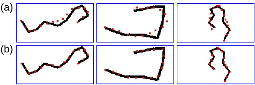
Figure 9: Visualizations of finetuning the predicted keypoints according to the surrounding geometric features. (a) Raw output of the network. (b) Finetuning results.

As discussed above, geometric finetuning is proposed to account for the residual error. Fig. 9(a) illustrates several failure cases, in which some detected keypoints drop out from the positive region of the DLO, mainly on the steep area of the curve. Comparatively, Fig. 9(b) visualizes the keypoints with finetuning, graphically indicating that this method improves the representation level of the sequential keypoints.

TABLE I: COMPARISON OF KEYPOINT DETECTION PERFORMANCE

	Corner Error $E_{C}$		Keypoint Error $E_{P}$
	$\mu_{C}$	$\sigma_{C}^{2}$	$\mu_{P}$	$\sigma_{P}^{2}$
Geo	1.96	29.78	28.21	389.96
Ours	1.71	12.5	3.36	21.44

• Geo: Geometric-based method; Our: Our data-driven algorithm. $\mu_{C},\sigma_{C}^{2}:$ Mean and variance of corner error $E_{C}$. $\mu_{P},\sigma_{P}^{2}:$ Mean and variance of keypointd error $E_{P}$.

Compared with data-driven learning models, manual designed descriptor is an alternative for keypoint detection due to its intuitiveness and interpretability. Here, we provide a comparison between our method and a traditional geometric-based baseline, whose steps include skeletonizing DLOs via [30] from $S^{[t]}$, searching the corners of DLOs according to the mesh grids, sorting and sampling the keypoints based on nearest neighbor search. Our error metrics include the corner $E_{C}$ and the keypoint detection error $E_{P}$, which are defined as $E_{C}=\frac{1}{2}(||\hat{p}_{1}-p_{1}||_{2}+||\hat{p}_{m}-p_{m}||_{2})$ and $E_{P}=\frac{1}{m}\sum_{j=1}^{j=m}||\hat{p}_{j}-p_{j}||_{2}$, respectively. We emphasize the corner error $E_{C}$ here since it is the symbol to order the keypoints. Statistically, we leverage the mean value ($\mu_{C},\mu_{P}$) and the variance ($\sigma_{C}^{2},\sigma_{P}^{2}$) to evaluate their performance comprehensively. Note that $p_{j}$ and $\hat{p}_{j}$ are the ground truth of the dataset and the output of the corresponding algorithm, respectively. The comparison results are shown in Table. I. Due to the huge diversity of the state space of DLOs, it is very difficult to manually develop a sequential keypoint detection method that is robust to various configurations. Conversely, our perception network is robust with its data-driven manner.

A key issue about descriptors is their representation level versus the original data. Since we only predict keypoints of DLOs based on the link-chain model, we reconstruct the original shape through end-to-end connection. For comparisons, we consider various unsupervised auto-encoders [12], whose goal is also to extract a compact latent code about the high-dimensional data. We choose three baselines to adapt to our case 1) fully connected linear regression (LR), 2) convolutional neural network (CNN), and 3) PointNet [31] (PC). Specifically, the training of LR and CNN autoencoders is conducted based on the binary cross entropy (BCE) loss $\mathcal{L}_{BCE}$, while PC autoencoder is optimized through Chamfer distance $d$. They are defined as:

$$\mathcal{L}_{BCE}=-\sum_{i=1}^{n}y_{i}\log\hat{y}_{i}+\left(1-y_{i}\right)\log\left(1-\hat{y}_{i}\right)$$ (16)

$$d\left(\hat{Y},Y\right)=\sum_{\hat{y}\in\hat{Y}}\min_{y\in Y}\|\hat{y}-y\|_{2}^{2}+\sum_{y\in Y}\min_{\hat{y}\in\hat{Y}}\|\hat{y}-y\|_{2}^{2}$$

According to the network structure, LR and CNN take the 2D image format as input while PC utilizes the 3D point cloud with the same size after down-sampling.

TABLE II: COMPARISON OF KEYPOINT DETECTION PERFORMANCE ON SYNTHETIC DATASET

	L1			IoU
Net	Train	Valid	Test	Train	Valid	Test
FCN-L	0.0074	0.0074	0.0073	0.6645	0.665	0.6648
FCN-R	0.0274	0.0276	0.0272	0.0798	0.0783	0.0804
FCN-F	0.0208	0.0212	0.0205	0.2558	0.2493	0.2573
LR	0.0297	0.0299	0.0325	0.0846	0.0852	0.0643
CNN	0.0294	0.0296	0.0291	0.0996	0.0995	0.0991
PC [31]	0.02	0.0201	0.0199	0.0882	0.0878	0.0852

• FCN-L: label of the FCN; FCN-R: raw output of the FCN; FCN-F: finetuning FCN; LR: linear regression; CNN: convolutional neural network; PC [31]: point cloud.

Since our original state $S^{[t]}$ is a binary image, the shape reconstruction issue here is formulated as a classification concerning each pixel $S^{[t]}(u,v)$. Hence, our evaluation metrics are L1 loss $\mathcal{L}_{1}$ and IoU (Intersection over Union) between the reconstructed output and the original information, respectively:

$$\mathcal{L}_{1}=\sum_{i=1}^{n}|y_{i}-\hat{y}_{i}|,IoU=\frac{\hat{y}\cap y}{\hat{y}\cup y}$$ (17)

Table. II shows the comparison results. Note that FCN-L method utilizes the labeled keypoints for reconstruction and acts as ground truth for our data-driven representation. The finetuning output of our perception improves greatly compared with the raw output of the network FCN-R. Compared with LR and CNN autoencoders, our proposed FCN-F performs better both in L1 loss and IoU. The main reason is that autoencoders aim to reconstruct the entire information of the input (even the details) instead of paying attention to the fundamental features. Although [31] achieves well in L1 loss, its performance concerning IoU is poor. This is because it is only able to reconstruct the original data with a fixed size (due to the identical input dimension); thus loses some information inevitably.

V-C Manipulation

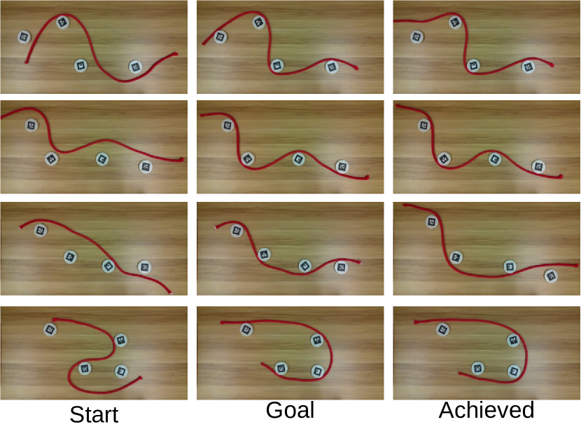
Figure 10: Our designed DLO manipulation with environmental contacts scenarios. From left to right: the start state, the goal state and achieved state with our framework. All the images are taken by our top-down Realsense L515 depth camera.

To validate our hierarchical action planning framework, we evaluate the performance with multiple experiments using various contact configurations and goals. Fig. 10 shows four designed tasks in our experiment. Note that the configuration of the DLO at the beginning $S^{[0]}$ is placed randomly on the table and the desired goal is provided artificially. For each experiment, we assume that the goal shape $S^{*}$ keeps stable with the support of the contacts and the table. The third column in Fig. 10 illustrates our achieved results. Since our hierarchical action planning is iterative, the robot continuously manipulates the DLO until the shape similarity between the goal $S^{*}$ and the achieved one $S^{[H]}$ is sufficient. In this experimental study, the shaping tasks are conducted with multi-step action depending on the feature extraction of the DLOs without learning their physical dynamics.

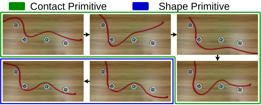
Figure 11: Our designed DLOs manipulation with environmental contacts scenarios. From left to right: the start state, the goal state and achieved state with our framework. All the images are taken by our top-down Realsense L515 depth camera.

As a multi-step decision-making process, we provide a typical example of the manipulation, as shown in Fig. 11. At the beginning, our algorithm computes the prior knowledge for the hierarchical action planning based on the goal image $I^{*}$: 1) segment the DLO $S^{*}$ with the color filter and detect the corresponding sequence ordered keypoints $P^{*}$ through our perception network and 2) localize the contacts $C=\{c_{1},\cdots,c_{k},\cdots,c_{q}\}$ and compute the contact-based benchmarks $(\mathcal{B},\mathcal{B}^{\prime},\mathcal{J})$. Then, our algorithm enters into the action loop. For each planning, we sense the DLO $S^{[t]}$ and detect its keypoints $P^{[t]}$ via our perception network. With this, we check the contact construction based on our search benchmarks $\mathcal{B}$. If it is failed, we utilize the contact primitive to construct the corresponding contact $c_{k}$. Once the action plan ($\mathcal{T}_{L},\mathcal{T}_{R}$) is accomplished, we update the state of the DLO $S^{[t+1]}$. If the contact restrictions are met, we move on to the shape primitive for finetuning. The entire algorithm iterates until reaching the goal state $S^{*}$, which the criteria is defined as the binary IoU between $S^{[t]}$ and $S^{*}$ according to Eq. 17 should be larger than $40\%$. We also provide supplementary material for robotic bimanual manipulation videos.

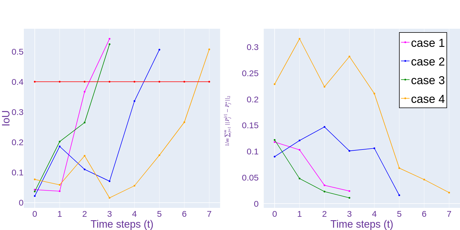
Figure 12: Shape error minimization process. (a) IoU between the goal state $S^{*}$ and the state $S^{[t]}$ in each time step $t$. (b) The keypoints error between $P^{*}$ and $P^{[t]}$.

Based on the goal shape in Fig. 10, we implement four trials under various initial configurations. Fig. 12 depicts the quantitative measurements of the scenarios in Fig. 10. Specifically, the minimization of the magnitude error $\Delta P$ is shown in Fig. 12(b). These results corroborate that the detected sequential keypoints can be used to manipulate the DLO into the desired specification. Fig. 12(a) demonstrates the similarity level of the state at each time step with the goal shape $S^{*}$, which IoU$=40\%$ serves as a baseline. Note that the IoU value decreases compared with the previous time step in some cases since the contact-based manipulation task is not continuous. Hence, a coarse-to-fine manner is necessary for this challenging task, otherwise, we probably get stuck in a local optimum. These results also reveal that our algorithm is superior in feature description and action planning versus this kind of challenging task.

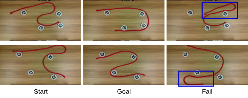
Figure 13: The stuck state of failure cases.

Although our planning framework is capable of dealing with the majority of these challenging tasks, there are some cases that the system fails. Fig. 13 presents two typical failure examples. Although our perception network plays well in most cases, its performance is severely affected by rolling. That is because the convolution is not good at dealing with the details of the pixels and the finetuning regresses the keypoints to the wrong region of the DLO, resulting in a sequence of disordered keypoints. Another case is caused by the lack of physical dynamics. Without any forecasting and feedback, our framework replans the action in an open-loop form. Thus, the system probably enters into a local convergence at the contacts.

VI CONCLUSIONS

In this paper, we demonstrate a keypoint-based bimanual manipulation for DLOs under environmental contact constraints. Training on a synthetic image dataset, our perception extracts sequential keypoints of DLOs as descriptors. The hierarchical action planning framework performs the task with two defined primitives in a coarse-to-fine manner. The whole algorithm is semantic without requiring any manual data collection and annotation. However, our methods exist some limitations. The perception network has poor performance in the knotted cases. As an open-loop method, the stability of the planner is not guaranteed. For future directions, we are interested to explore the synergistic behaviors between dual arms to extend the framework for other deformable objects, such as clothes and bags.

References

- [1] J. Zhu, B. Navarro, P. Fraisse, A. Crosnier, and A. Cherubini, “Dual-arm robotic manipulation of flexible cables,” in 2018 IEEE/RSJ International Conference on Intelligent Robots and Systems (IROS), pp. 479–484, IEEE, 2018.
- [2] I. Garcia-Camacho, M. Lippi, M. C. Welle, H. Yin, R. Antonova, A. Varava, J. Borras, C. Torras, A. Marino, G. Alenya, et al., “Benchmarking bimanual cloth manipulation,” IEEE Robotics and Automation Letters, vol. 5, no. 2, pp. 1111–1118, 2020.
- [3] D. Navarro-Alarcon, H. M. Yip, Z. Wang, Y.-H. Liu, F. Zhong, T. Zhang, and P. Li, “Automatic 3-d manipulation of soft objects by robotic arms with an adaptive deformation model,” IEEE Transactions on Robotics, vol. 32, no. 2, pp. 429–441, 2016.
- [4] K. Galassi and G. Palli, “Robotic wires manipulation for switchgear cabling and wiring harness manufacturing,” in 2021 4th IEEE International Conference on Industrial Cyber-Physical Systems (ICPS), pp. 531–536, IEEE, 2021.
- [5] J. Sanchez, J.-A. Corrales, B.-C. Bouzgarrou, and Y. Mezouar, “Robotic manipulation and sensing of deformable objects in domestic and industrial applications: a survey,” The International Journal of Robotics Research, vol. 37, no. 7, pp. 688–716, 2018.
- [6] D. Navarro-Alarcon, Y.-H. Liu, J. G. Romero, and P. Li, “Model-free visually servoed deformation control of elastic objects by robot manipulators,” IEEE Transactions on Robotics, vol. 29, no. 6, pp. 1457–1468, 2013.
- [7] J. Zhu, D. Navarro-Alarcon, R. Passama, and A. Cherubini, “Vision-based manipulation of deformable and rigid objects using subspace projections of 2d contours,” Robotics and Autonomous Systems, vol. 142, p. 103798, 2021.
- [8] D. Navarro-Alarcon and Y.-H. Liu, “Fourier-based shape servoing: a new feedback method to actively deform soft objects into desired 2-d image contours,” IEEE Transactions on Robotics, vol. 34, no. 1, pp. 272–279, 2017.
- [9] J. Zhu, A. Cherubini, C. Dune, D. Navarro-Alarcon, F. Alambeigi, D. Berenson, F. Ficuciello, K. Harada, X. Li, J. Pan, et al., “Challenges and outlook in robotic manipulation of deformable objects,” arXiv preprint arXiv:2105.01767, 2021.
- [10] Z. Wang, X. Li, D. Navarro-Alarcon, and Y.-h. Liu, “A unified controller for region-reaching and deforming of soft objects,” in 2018 IEEE/RSJ International Conference on Intelligent Robots and Systems (IROS), pp. 472–478, IEEE, 2018.
- [11] D. Navarro-Alarcon, Y.-h. Liu, J. G. Romero, and P. Li, “On the visual deformation servoing of compliant objects: Uncalibrated control methods and experiments,” The International Journal of Robotics Research, vol. 33, no. 11, pp. 1462–1480, 2014.
- [12] P. Zhou, J. Zhu, S. Huo, and D. Navarro-Alarcon, “Lasesom: A latent and semantic representation framework for soft object manipulation,” IEEE Robotics and Automation Letters, 2021.
- [13] T. Tang, C. Wang, and M. Tomizuka, “A framework for manipulating deformable linear objects by coherent point drift,” IEEE Robotics and Automation Letters, vol. 3, no. 4, pp. 3426–3433, 2018.
- [14] D. Tanaka, S. Arnold, and K. Yamazaki, “Emd net: An encode–manipulate–decode network for cloth manipulation,” IEEE Robotics and Automation Letters, vol. 3, no. 3, pp. 1771–1778, 2018.
- [15] E. Johns, S. Leutenegger, and A. J. Davison, “Deep learning a grasp function for grasping under gripper pose uncertainty,” in 2016 IEEE/RSJ International Conference on Intelligent Robots and Systems (IROS), pp. 4461–4468, IEEE, 2016.
- [16] D. Seita, A. Ganapathi, R. Hoque, M. Hwang, E. Cen, A. K. Tanwani, A. Balakrishna, B. Thananjeyan, J. Ichnowski, N. Jamali, et al., “Deep imitation learning of sequential fabric smoothing from an algorithmic supervisor,” in 2020 IEEE/RSJ International Conference on Intelligent Robots and Systems (IROS), pp. 9651–9658, IEEE, 2020.
- [17] P. Sundaresan, J. Grannen, B. Thananjeyan, A. Balakrishna, M. Laskey, K. Stone, J. E. Gonzalez, and K. Goldberg, “Learning rope manipulation policies using dense object descriptors trained on synthetic depth data,” in 2020 IEEE International Conference on Robotics and Automation (ICRA), pp. 9411–9418, IEEE, 2020.
- [18] M. Yan, Y. Zhu, N. Jin, and J. Bohg, “Self-supervised learning of state estimation for manipulating deformable linear objects,” IEEE robotics and automation letters, vol. 5, no. 2, pp. 2372–2379, 2020.
- [19] S. Jin, C. Wang, and M. Tomizuka, “Robust deformation model approximation for robotic cable manipulation,” in 2019 IEEE/RSJ International Conference on Intelligent Robots and Systems (IROS), pp. 6586–6593, IEEE, 2019.
- [20] T. Tang and M. Tomizuka, “Track deformable objects from point clouds with structure preserved registration,” The International Journal of Robotics Research, p. 0278364919841431, 2018.
- [21] H. Yin, A. Varava, and D. Kragic, “Modeling, learning, perception, and control methods for deformable object manipulation,” Science Robotics, vol. 6, no. 54, 2021.
- [22] L. P. Kaelbling and T. Lozano-Pérez, “Hierarchical task and motion planning in the now,” in 2011 IEEE International Conference on Robotics and Automation, pp. 1470–1477, 2011.
- [23] A. M. Wells, N. T. Dantam, A. Shrivastava, and L. E. Kavraki, “Learning feasibility for task and motion planning in tabletop environments,” IEEE robotics and automation letters, vol. 4, no. 2, pp. 1255–1262, 2019.
- [24] J. Zhu, B. Navarro, R. Passama, P. Fraisse, A. Crosnier, and A. Cherubini, “Robotic manipulation planning for shaping deformable linear objects withenvironmental contacts,” IEEE Robotics and Automation Letters, vol. 5, no. 1, pp. 16–23, 2019.
- [25] M. Wnuk, C. Hinze, A. Lechler, and A. Verl, “Kinematic multibody model generation of deformable linear objects from point clouds,” in 2020 IEEE/RSJ International Conference on Intelligent Robots and Systems (IROS), pp. 9545–9552, IEEE, 2020.
- [26] P. Song and V. Kumar, “A potential field based approach to multi-robot manipulation,” in Proceedings 2002 IEEE International Conference on Robotics and Automation (Cat. No. 02CH37292), vol. 2, pp. 1217–1222, IEEE, 2002.
- [27] G. Bradski, “The opencv library,” Dr Dobb’s J. Software Tools, vol. 25, pp. 120–125, 2000.
- [28] J. Long, E. Shelhamer, and T. Darrell, “Fully convolutional networks for semantic segmentation,” in Proceedings of the IEEE conference on computer vision and pattern recognition, pp. 3431–3440, 2015.
- [29] K. Simonyan and A. Zisserman, “Very deep convolutional networks for large-scale image recognition,” arXiv preprint arXiv:1409.1556, 2014.
- [30] T. Y. Zhang and C. Y. Suen, “A fast parallel algorithm for thinning digital patterns,” Communications of the ACM, vol. 27, no. 3, pp. 236–239, 1984.
- [31] P. Achlioptas, O. Diamanti, I. Mitliagkas, and L. Guibas, “Learning representations and generative models for 3d point clouds,” in International conference on machine learning, pp. 40–49, PMLR, 2018.