On the dynamics of the contagious rate under isolation measures

Abstract

The infection dynamics of a population under stationary isolation conditions is modeled. It is underlined that the stationary character of the isolation measures can be expected to imply that an effective SIR model with constant parameters should describe the infection process. Then, a derivation of this property is presented, assuming that the statistical fluctuations in the number of infection and recovered cases are disregarded. This effective SIR model shows a reduced population number and a constant $\beta$ parameter. The effects of also including the retardation between recovery and infection process is also considered. Next, it is shown that any solution of the effective SIR also solves the linear problem to which the SIR equations reduce when the total population is much larger than the number of the infected cases. Then, it is also argued that this equivalence follows for a specific contagious parameter $\beta(t)$ which time dependence is analytically derived here. Then, two equivalent predictive calculational methods for the infection dynamics under stationary isolation measures are proposed. The results represent a solutions for the known and challenging problem of defining the time dependence of the contagion parameter, when the SIR parameter $N$ is assumed to be the whole population number. Finally, the model is applied to describe the known infection curves for countries that already had passed the epidemic process under strict stationary isolation measures. The cases of Iceland, New Zealand, Korea and Cuba were considered. Although, non subject to stationary isolation measures the cases of U.S.A. and Mexico are also examined due to their interest. The results support the argued validity of SIR model including retardation.

I Introduction

As following from its relevance for the human beings, the investigation of the covid-19 epidemic had attracted a lot of attention in the actual research literature 1 ; 2 ; 3 ; 4 ; 5 ; 6 ; 7 ; 8 ; 9 ; 10 ; 11 ; ours ; 12 ; 13 ; DamianNana ; harko ; 14 ; 15 ; 16 ; 17 ; 18 ; 19 . Currently, a large number of information centers publish the epidemic data which are reported daily for almost all the counties in the planet 9 , 11 . This situation furnish to the researchers abundant information about the pandemic.

In a previous work in reference ours we had underlined the interest of considering the dynamics of the contagion parameter $\beta$ of the SIR model under isolation measures over the populations. As it is known, this model is one of the main ones in epidemiology. It has the whole number of habitants $N_{pop}$ as one of its parameters. Therefore, if the population of the country $N_{pop}$ is assumed as the $N$ parameter, and the number of infected cases is very much smaller than $N_{pop},$ the linearity of the equations enforces that the model parameters should change in time as a consequence of the imposed isolation measures, if maxima of the infected cases appear. In that work, we formulated a model in which the initially constant contagion parameter $\beta$ suddenly drops to a smaller value just after the isolation measures are installed. Further, it was assumed that these measures should also continuously reduce the value of the contagion parameter. This was expected to occur because the infected persons will be confined from to be in contact with most of the other persons. Thus, they can infect only close members of the family, and only up to the mean time for which the infected person remains sick. But, considering the unreal limit of all the habitants being isolated one from any other, it is clear that the contagion parameter should become exactly zero after a mean time of occurrence of the affection. Therefore, we fixed the parameter $\beta$ drastically to zero after a mean time of duration of the sickness following the imposition of the confinement rules. This assumption was taken only for countries in which the isolation measures had been rigorously and stationary maintained, as in Germany. The application of this simple model was able to appropriately describe the curve of infection for this country ours .

In the present work, we investigate the infection process as occurring in countries in which strict isolation measures had been taken, showing a stationary in time character. That is, measures that remain applied during a time lapse without serious modifications which could change the contagion dynamics in the Society.

The work firstly presents a proof that, under the above conditions, the epidemic should be described by an effective SIR process, having a reduced population number parameter, as well as a contagion $\beta$ one. The recovering parameter, can not be expected to be altered by the isolation measures, since it only depends of the society structure and the established action of the Health System of each country.

Also, the discussion considers the incorporation of the retardation between the recovery and the infection of the affected persons. The effect was described by a new retardation time parameter $\tau.$ This consideration should be taken into account for describing the epidemic data reported 7 .

In addition it was took into account a characteristic property of the covid-19 epidemic. It is the large number of persons which shows the sickness in a mild form, not allowing them to be detected by the Health Systems. It is then considered that the observed data of infected persons is a definite fraction $k$ of the total number of infected persons 5 . This fraction had been estimated to have a value nearly to $k=0.2$. This effect is used to define the initial conditions of the SIR model equations in terms of the observed data.

A second main aim of this study consists in to discuss the SIR models assuming that the parameter $N$ represents the total population of the country and the number of infected cases is very much smaller than $N$. It can underlined that this class of studies had been widely considered in epidemiology research along the times 14 ; 15 ; 16 ; 17 ; 18 ; 19 . In them, it had been always unclear how to define the required time dependence of the contagion parameter which becomes required if the epidemic evolutions show maxima which are very much smaller than the country population. It should be noted that when the parameter $N$ is the total population and the number of infected persons is still very much smaller than $N$, the SIR equations become linear, and not showing any maxima as time follows if the parameters of the model are strictly constant ours . The present work intends to clarify this situation by identifying the time dependent contagion parameter which should be assumed in order to define the solution of the linear model describing the evolution of the epidemic under stationary isolation conditions.

For the above defined purpose, it is firstly shown that solutions of the effective SIR equations $S_{e}(t),I_{e}(t)$ and $R_{e}(t)$ are also solutions of the linear SIR equations for large populations and small number of infected persons for special definite time dependent contagion parameter $\beta(t)$. Further, this time dependent $\beta(t)$ is exactly evaluated as a function of the parameters $N_{e}$, $\beta_{e}$ and $\gamma$ of the effective SIR. Therefore, the time dependence of the contagion parameter required for defining the epidemic evolution under isolation conditions of the populations is exactly determined, for the situation in which the parameter $N$ of the SIR model is made equal to the population number.

Finally, the model including retardation is applied to the reported infection data for various countries. The epidemic data were mainly collected from reference 9 . The effective SIR equations including retardation were firstly applied to Iceland and New Zealand. These two countries are known by their effective isolation measures that were able to finish the epidemic. After, fixing the initial data for the confirmed, infected and recovered cases, it was possible to determine the four parameters of the model ($\beta$, $N$, $\gamma$ and $\tau$). They were chosen in order to define a solution for the equations which closely resembles the observed data presented in reference 9 for those two countries. The result confirms that the SIR equations are closely satisfied by the infection dynamics under stationary isolation conditions. Further, it was investigated the epidemic infection curve associated to South Korea. Following the same procedure as for Iceland and New Zealand, the solution determined by the reported initial data, also closely approached the data curves for confirmed, infected and recovered cases up to the 4 March 2020. After this time the solutions deviated form the measured data. Then, the information on the isolation measures for South Korea was consulted. With surprise, we found that precisely the 4 March the government of the country had enforced new drastic isolation measures, which had disrupted the stationary property of the before taken rules. Therefore, a clear explanation emerged for the observed deviation of the SIR solution from the data after the 4 March. Next, the case of Cuba was also studied. The stationary character of the applied rules was also checked since the data were also closely matching by a definite solution of the SIR equations including retardation.

It should be underlined that in all the above mentioned countries, non vanishing retardation between the recovery and infection were needed to closely approach the observed data. Also, the recovery rate parameters determined for optimally approaching the observed data were also closely near the value 0.05.

We applied to model to the case of United States and Mexico. The epidemic had taken its strongest form in USA at the time of ending the writing of this work. In Mexico, a large country, the epidemic had taken an irregular evolution. Therefore, we decided to explore the possibility of estimating the infection curves for both countries. However, it can not be assured that U.S.A. and Mexico had established well defined stationary and globally applied isolation measures. Thus, the present exploration should be only considered as a possibly helpful rough estimation of an important information for these two strong epidemics.

The work proceeds as follows. In Section 2, it is presented the argue about that the SIR model with modified parameters should be valid for describing the stationary isolation infection measurements. It is also introduced the retardation of the SIR equations, which should be expected to be relevant in comparing the solutions with the observed data.

Further, initial conditions for the SIR equations appropriately describing the large number of asymptomatic cases in the covid-19 epidemic are defined in Section 3.

Next, the Section 4 shows that the effective SIR solutions also solve the linear SIR equations for small ratio between the number of infected cases and the total population.

The solutions of the equations are considered in various subsections of Section 5, in order to compare the predictions of the SIR model with retardation with the observed infection data in the literature for various countries. The conclusions shortly resume the results of the paper and mention possible extensions.

II Populations under stationary isolation measures

Let us assume that the country population $N$ is grouped in families having a probability distribution of having a specified number of elements in the family. Just after the given time of imposition of the isolation measures, there will be a number of infected persons, that will be localized in a number of families $F_{\inf}$ . They will be called as infected families. The rest of families $F_{hea}=F-F_{\inf}$ will be named as healthy ones. But, since the isolation conditions will be assumed to avoid the contagious between families, the number $F_{hea}$ should expected to be nearly constant in time, as it will be also the number of infect ones $F_{\inf}.$ These nearly conserved numbers can be suspected as defining the new effective population parameter.

Let us separately consider in what follows the evaluations of the rate of infection of the susceptible persons and the rate of recuperation of the cases.

II.1 The recuperation rate

This is the most simple of the quantities to determine, because it is reasonably to consider it as well described by same equation valid for the SIR model

$$R(t)=\gamma\text{ }I(t),$$ (1)

where numerical estimates of the recuperation rate parameter $\gamma$ exist in the literature. This constant in time rate is expected to be valid because the isolation conditions should not change the probability of recuperation of a given infected person as randomly determined in mean by his physiology and the standard treatments of the Health System in his country.

II.2 The infection rate

Let us consider now the infection rate under isolation conditions. For this purpose define the number of infected persons $n_{i}$ in each infected family with the subindex $i$, running over $i=1,2,3,....,F_{\inf}.$ The total number of members of each family will be indicated by $j_{i}$

Consider now a given infected person in his neighborhood of $j_{i}$ familiar persons and define the probability $p$ that he infects another person during a day interval (the unit of time assumed). Consider also that in any family $i$ there are $n_{i}^{R}$ recuperated members in addition to the $n_{i}$ infected ones. In these conditions there will be $(j_{i}-$ $n_{i}-n_{i}^{R})$ remaining susceptible members.

Then, the probability that a given sick person infects within a day a member of his family can estimated by the product of the probability for infecting a person by the number of susceptible persons in the family. Since there are $n_{i}$ infected persons in the family, the probability should be also multiplied by $n_{i}$. Then, it results that the change in the number of susceptible persons $S^{\ast}$ per unit time can be estimated in the form

$$\frac{dS^{\ast}(t)}{dt}=-\sum_{i}n_{i}\text{ }p\text{ }(j_{i}-n_{i}-n_{i}^{R}).$$ (2)

Define now the mean numbers of infected $\overline{n}(t)$ and recovered $\overline{n}^{R}(t)$ persons, and the mean number of elements in the infected families $n$ at a given time $t$ as

$$\overline{n}(t) =\frac{1}{F_{\inf}}\sum_{i}n_{i}(t)=\frac{1}{F_{\inf}}I(t),$$ (3)

$$\overline{n}^{R}(t) =\frac{1}{F_{\inf}}\sum_{i}n_{i}^{R}(t)=\frac{1}{F_{\inf}}R(t),$$ (4)

$$n =\frac{1}{F_{\inf}}\sum_{i}j_{i}.$$ (5)

Then, we can write $\frac{dS^{\ast}(t)}{dt}$ in the form

$$\frac{dS^{\ast}(t)}{dt} =-\sum_{i}n_{i}\text{ }p\text{ }(j_{i}-n_{i}-n_{i}^{R})$$

$$=-F_{\inf}\text{ }n\text{ }p\text{ }\overline{n}(t)+p\sum_{i}(n_{i}^{2}\text{ }+n_{i}n_{i}^{R})$$

$$=-\text{ }n\text{ }p\text{ }I(t)+p\sum_{i}(n_{i}^{2}\text{ }+n_{i}n_{i}^{R}).$$ (6)

The first term in the last line of equation (6) is already expressed in terms of the whole number of infected persons $I(t)$ as in the SIR equations. However, the second term is a sum of quadratic terms in the numbers of infects and recuperated persons in the families.

But, it is possible to write for them

$$\sum_{i}n_{i}^{2} =\sum_{i}(n_{i}-\text{ }\overline{n}(t)+\text{ }\overline{n}(t))^{2}$$

$$=\sum_{i}(n_{i}-\text{ }\overline{n}(t))^{2}+\text{ }\overline{n}(t)^{2}+2\text{ }\overline{n}(t)(n_{i}-\text{ }\overline{n}(t))$$

$$=\text{ }\overline{n}(t)^{2}+\sum_{i}(n_{i}-\text{ }\overline{n}(t))^{2},$$ (7)

$$\sum_{i}n_{i}n_{i}^{R} =\sum_{i}(n_{i}(t)-\text{ }\overline{n}(t)+\text{ }\overline{n}(t))(n_{i}^{R}-\text{ }\overline{n}^{R}(t)+\text{ }\overline{n}^{R}(t))$$

$$=\text{ }\overline{n}(t)\overline{n}^{R}(t)+(n_{i}(t)-\text{ }\overline{n}(t))(n_{i}^{R}(t)-\text{ }\overline{n}^{R}(t))+$$

$$(n_{i}(t)-\text{ }\overline{n}(t))\overline{n}^{R}(t)+\overline{n}(t)(n_{i}^{R}(t)-\text{ }\overline{n}^{R}(t))$$

$$=\overline{n}(t)\overline{n}^{R}(t)+(n_{i}(t)-\text{ }\overline{n}(t))(n_{i}^{R}(t)-\text{ }\overline{n}^{R}(t)).$$ (8)

We will consider that the number of infected $n_{i}$ and recovered $n_{i}^{R}$ persons in the number of infected families show small deviations from the respective mean numbers $\overline{n}(t)$ and $\overline{n}^{R}(t)$. That is, the following relations are obeyed

$$|n_{i}(t)-\text{ }\overline{n}(t)|\text{ } \ll\text{ }\overline{n}(t),$$

$$|n_{i}^{R}(t)-\text{ }\overline{n}^{R}(t)|\text{ } \ll\text{ }\overline{n}^{R}(t).$$

Therefore, the statistical fluctuations in those number may be disregarded.

Under these assumption the expression (6) can be written only in terms of the mean numbers of infected and recovered cases as

$$\frac{dS^{\ast}(t)}{dt} =-n\text{ }p\text{ }I(t)+pF_{\inf}(\overline{n}^{2}\text{ }+\overline{n}\text{ }\overline{n}^{R})$$ (9)

$$=-n\text{ }p\text{ }I(t)+pF_{\inf}((\frac{I(t)}{F_{\inf}})^{2}\text{ }+\frac{I(t)}{F_{\inf}}\frac{R(t)}{F_{\inf}})$$ (10)

$$=-p\text{ }I(t)\text{ }{\Large(}n-\frac{I(t)}{F_{\inf}}-\frac{R(t)}{F_{\inf}}{\large).}$$ (11)

Thus, it is possible to write now the set of equations for the system. After considering the exact relation

$$N=S^{\ast}(t)+I(t)+R(t),$$ (12)

which implies

$$\frac{dI(t)}{dt}=-\frac{dS^{\ast}(t)}{dt}-\frac{dR(t)}{dt},$$ (13)

and employing (3), (4), (5) and (6), the set of equations for modeling the isolation condition of the population can be written as follows

$$\frac{dS^{\ast}(t)}{dt} =-p\text{ }{\Large(}n-\frac{I(t)}{F_{\inf}}-\frac{R(t)}{F_{\inf}}{\large)}\text{ }I(t),$$ (14)

$$\frac{dI(t)}{dt} =p\text{ }{\Large(}n-\frac{I(t)}{F_{\inf}}-\frac{R(t)}{F_{\inf}}{\large)}\text{ }I(t)-\gamma I(t),$$ (15)

$$\frac{dR(t)}{dt} =\gamma I(t).$$ (16)

But, we can define the new quantities

$$\ N =n\text{ }F_{\inf}<N_{pop},$$ (17)

$$\beta =\frac{p}{F_{\inf}},$$ (18)

where the total population of the country had been called $N_{pop}$ . It is larger than the number of persons $n$ $F_{\inf}$ living in the $F_{\inf}$ infected families. In terms of these constants the set of equations (14,15,16) can be finally rewritten in the typical SIR form

$$\frac{dS^{\ast}(t)}{dt} =-\beta\text{ }{\Large(}N-I(t)-R(t){\large)}\text{ }I(t),$$ (19)

$$\frac{dI(t)}{dt} =\beta\text{ }{\Large(}N-I(t)-R(t){\large)}\text{ }I(t)-\gamma I(t),$$ (20)

$$\frac{dR(t)}{dt} =\gamma I(t).$$ (21)

Therefore, it was argued that a system under stationary isolation condition should also satisfy the SIR equations when the statistical fluctuations on the number of infected and recovered cases can be disregarded. This assumption can be expected to be obeyed for large populations. This result implies that the infection of countries under stationary isolation measures can be exactly described by a SIR model with modified parameters, such that the $N$ parameter is lower than the total number of habitants in the country.

II.3 Retardation effects

Before adopting the final form of the equations for the model, we estimate that it should be also taken into account that there is a time interval that should pass after the infection day, in order that a given person recovers the healthy state. Clearly, this time is an stochastic quantity which can not be precisely defined. However, we will attempt to describe this effect by assuming a definite mean time interval for recovery. It also becomes clear that for epidemics which appear and disappear within a short time period, this effect can have a more important influence on the dynamics of the process. In order to consider this element, we will introduce in the proposed a model a retardation effect. It will be approximately considered that the rate of recovering at a given time $t$ is proportional not to the number of infected persons at this same time, but at a past time $t-\tau.$ The parameter $\tau$ is assumed to be fixed in order to simplify the discussion of the stochastic nature of the retardation effects.

Finally, the system of equation including these effects will be considered in the form

$$\frac{\partial S^{\ast}(t)}{\partial t} =-\beta\text{ }S^{\ast}(t)\text{ }I(t),$$ (22)

$$\frac{\partial I}{\partial t} =\beta\ \ S^{\ast}(t)\text{ }I(t)-\gamma\text{ }I(t-\tau),$$ (23)

$$\frac{\partial R}{\partial t} =\gamma\text{ }I(t-\tau),$$ (24)

which retains valid the general conservation relation

$$N=S^{\ast}(t)+I(t)+R(t).$$ (25)

It will be helpful to also write the equation in terms of the so called logistic equation by defining the quantity

$$S(t)=I(t)+R(t).$$

Then, the final equations to be further employed take the expression

$$\frac{dS(t)}{dt} =\beta(N-S(t))I(t),$$ (26)

$$\frac{dI}{dt} =\beta\ (N-S(t))I(t)-\gamma I(t-\tau),$$ (27)

$$\frac{dR}{dt} =\gamma I(t-\tau).$$ (28)

III Initial conditions and the symptomatic to total cases ratio.

We will write a set of initial conditions being appropriate to the situation at any initial moment being after the specific day at which isolation period is established. Let us call $t_{o}$ a date at which the initial conditions are imposed. After that, the isolation measures are assumed to be maintained in a stationary form for the whole population. Assuming numbers of susceptible $S$, infected $I$ and recovered $R$ persons as functions of time, we can write for the initial conditions of the set of retarded equations (26,27,28) for the model

$$I(t) =I(t)\text{ \ \ for all \ \ }t\leq t_{o},$$ (29)

$$R(t_{o}^{+}) =R(t_{o}^{-}),$$ (30)

$$S(t_{o}^{+}) =S(t_{o}^{-}).$$ (31)

Since the only retarded quantity is the active infected number, the already measured values of the quantity $I(t)$ at all times $t\leq t_{o}$ are assumed as initial conditions for the set of equations.

One important point should be also considered: the ratio $k$ between the observed number of infected persons and the total number of them is being a number smaller than unit. We will use for defining it, the evaluation given in the literature that nearly the 80 % of the infected persons are asymptomatic 5 . That is, they show the sickness in a mild form which is not detected by the Health Systems. Then, we will assume the value

$$k=0.2,$$ (32)

for the ratio between the number of detected symptomatic cases and the total number of cases.

Since the quantities entering the equations (26,27,28) will be considered defining the total number of confirmed $S$, active $I$ and recovered $R$ cases, the initial conditions will be defined in the form

$$S(t_{o}) =\frac{S_{obs}(t_{o})}{k},$$ (33)

$$I(t) =\frac{I_{obs}(t)}{k}\text{ \ \ for all \ \ }t\leq t_{o},$$ (34)

$$R(t_{o}) =\frac{R_{obs}(t)}{k},$$ (35)

where $S_{obs}(t)$, $I_{obs}(t)$ and $R_{obs}(t)$ are the observed numbers of confirmed, active infected and recovered cases, respectively. These numbers after divided by $k$ give the corresponding numbers of total cases which are the quantities for which the SIR with retardation equations were derived.

In order to define a smaller range of values for the free parameter $N$ we will also employ in place of it, the quantity

$$n_{m}=\frac{N}{\frac{I_{obs}(t_{o})}{k}},$$ (36)

which is the mean number of infected family members as defined in (5), after assuming that at the initial time $t_{o}$ any infected family have at most only one infected person. That is, $F_{inf}=\frac{I_{obs}(t_{o})}{k}$ . This interpretation seems reasonable at an initial time where the number of infected persons is very much smaller than the whole population.

In the final section we will solve the set of equations (26,27,28) in order to check the applicability of the model in reproducing the  infection data already measured for various countries. Most of the countries considered will be ones in which well defined isolation measures were adopted which were maintained stationary in time.

IV Small number of cases solutions: link with the linear model at large populations

In this section we will clarify the links between the effective SIR solutions for epidemics in which the total number of infected persons is very much smaller than the total population of the country and the solutions for SIR for the total population number. When the number of infected persons is very much smaller than the population, the SIR for the total population reduces to a linear system of differential equations ours . But, if the parameters are constant, the solutions become exponentials which decrease, increase or remain constant all the time. Thus, the only way of describing maxima of the infection curves is by assuming a time dependence of the parameters. However, as it was mentioned before, the recovery rate $\gamma$ is naturally expected to remain constant, because it should only depend on the standard medical treatments of the Health System of the population, in a given country. Thus, the maxima of the infection curves for many countries in which the number of cases is very much lower than the population, must be necessarily attained by assuming a time dependent contagion rate $\beta(t).$

Below, it will shown that for each solution of the effective SIR equations with constant parameters, the time dependent numbers of susceptible, infected and recovered cases, also exactly satisfy the SIR for the total population, but for a time dependent contagion rate $\beta(t)$. The explicit analytic formula of $\beta(t)$ is derived here.

Consider the effective SIR equations with time dependent contagion rate $\beta(t)$, for the whole population number (27)

$$\frac{dI}{dt}=\beta(t)(N-S(t))I(t)-\gamma I(t-\tau),$$ (37)

in which the parameter $N$ is the population number of a country, and assume that the total number of infected cases $S(t)=I(t)+R(t)$ up to a given time $t$, satisfies

$$I(t)+R(t)\ll N.$$

Then, the SIR equations reduce to the linear differential equation

$$\frac{dI}{dt}=\beta(t)\text{ }N\text{ }I(t)-\gamma I(t-\tau).$$ (38)

IV.1 The effective SIR equations

Let us now consider a solution of the effective SIR equations with constant parameters $(N_{e},\beta_{e})$ written in the form

$$\frac{dS_{e}(t)}{dt} =\beta_{e}(N_{e}-S_{e}(t))I_{e}(t),$$ (39)

$$\frac{dI_{e}(t)}{dt} =\beta_{e}\ (N_{e}-S_{e}(t))I_{e}(t)-\gamma I_{e}(t-\tau),$$ (40)

$$\frac{dR_{e}(t)}{dt} =\gamma I_{e}(t-\tau),$$ (41)

in which the recovery rate $\gamma$ is common with the one in (38).

Then, if the following relation is exactly satisfied

$$\beta(t)\text{ }N=\beta_{e}\ (N_{e}-S_{e}(t)),$$

the solution ($S_{e}(t)),I_{e}(t),R_{e}(t))$ of the effective SIR equations is also a solution of linear SIR equations for the total population. But, employing (40) the analytic time dependence of the contagion parameter takes the form

$$\beta(t)\text{ }=\frac{1}{N}(\frac{1}{I_{e}(t)}\frac{dI_{e}(t)}{dt}+\gamma).$$ (42)

This time dependence is furnished by the known parametric explicit solution of the SIR equations with constant parameters (See reference harko ), which we reproduce below for completeness. The number of susceptible $S_{e}$, infected $I_{e}$ and $R_{e}$ cases infected and the time $t$, are defined as functions of the parametric function $s_{\eta}(t)$ by the relations harko

$$t = \int_{\exp(-\frac{\beta}{\gamma}n_{3})}^{s_{\eta}(t)}\frac{ds}{s(-\beta_{e}\text{ }N_{e}-\gamma\ln(s)+\chi_{0}\beta_{e}\text{ }s)},$$ (43)

$$S_{e}(t) = \chi_{0}\text{ }s_{\eta}(t),$$ (44)

$$I_{e}(t) = \frac{\gamma}{\beta_{e}}\ln(s_{\eta}(t))-\chi_{0}\text{ }s_{\eta}(t)+N_{e},$$ (45)

$$R_{e}(t) = -\frac{\gamma}{\beta_{e}}\ln(s_{\eta}(t)),$$ (46)

in which $\eta=(\beta,\gamma,N_{e},n_{1},n_{2}.n_{3})$ is the set of free parameters of the solution, and the initial conditions had been fixed as

$$S_{e}(0) = n_{1},$$ (47)

$$I_{e}(0) = n_{2},$$ (48)

$$R_{e}(0) = n_{3},$$ (49)

$$N_{e} = n_{1}+n_{2}+n_{3}.$$ (50)

In the above relations the constants $\chi_{0}$ is defined by the relation

$$\chi_{0}=n_{1}\exp(\frac{\beta}{\gamma}n_{3}).$$

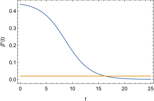
Figure 1: The curve gives the time dependence of the contagion parameter $\beta(t)$. This function after substituted in the linear equations for the SIR for total population, allows that the solutions of the effective SIR equations for the same parameter values also satisfy them. The function depends on the parameters and initial conditions of the effective SIR equations. These values can be varied in order to find the specific time dependence which closely fits the data for the susceptible, infected and recovered cases at the beginning of the infection. Then, for future times, the solution can be compared with the data to be taken.

Making use of these definitions, the expression for the time dependent contagion parameter (42) and the function $R_{0}(t)$ may be written as

$$N\beta(t) =\beta^{\ast}(t)=\beta_{e}n_{1}\exp(\frac{\beta_{e}}{\gamma}n_{3})\text{ }s_{\eta}(t),$$ (51)

$$R_{0}(t) =\frac{\beta^{\ast}(t)}{\gamma}=\frac{1}{\gamma}\frac{1}{I_{e}(t)}\frac{dI_{e}(t)}{dt}+1$$

$$=\frac{1}{\gamma}\beta_{e}n_{1}\exp(\frac{\beta_{e}}{\gamma}n_{3})\text{ }s_{\eta}(t).$$ (52)

The figure 1 shows the time dependent $\beta(t)$ for which the effective SIR solutions associated to the specific parameter values

$$\eta = (\beta,\gamma,N_{e},n_{1},n_{2}.n_{3})$$ (53)

$$= (0.01,0.02,45,44,1,0).$$

The horizontal line plots the constant value of $\gamma$ and the intersection point defines the maximum of the curve of active infected cases.

IV.2 Proposals for predictive time dependence methods for epidemics

The results of this section can be used for attempting to predict the epidemics in the cases that rigorous stationary isolation measures had been imposed in the Society. The method only will be sketched here, but it will be investigated in more detail elsewhere. Under the stationary assumption, we had argued in the first Section that a SIR model should define the time evolution of the infection. The method can be easily described by examining figure 2. It plots the SIR model solution (47,48,49) for the particular set of parameters and initial conditions

$$\eta =(\beta,\gamma,N_{e},n_{1},n_{2}.n_{3})$$

$$=(0.01,0.02,45,44,1,0).$$ (54)

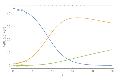
Figure 2: The solution for susceptible $S_{e}(t)$, infected $I_{e}(t)$ and recovered $R_{e}(t)$ cases for the effective SIR model. They are associated to the parameters chosen in (53) for evaluating the $\beta^{*}(t)$. The point plots near the initial time $t=0$ are only auxiliary illustrations representing the observed data for each of the three quantities $S_{e}(t)$, $I_{e}(t)$ and $R_{e}(t)$.

The figure shows the susceptible $S_{e}(t)$, infected $I_{e},$ and recovered $R_{e}$ number of particles solving the effective SIR equations.

Let us assume now that the Health systems had observed the three types of numbers during a given time interval at the beginning of the epidemics. These measured numbers are symbolized by the irregularly distributed points being close to the three continuous solutions of the model. Then, the discussion in this paper allows shows that for describing the epidemics under stationary isolation measures, it is possible two use two methods. Let us describe them below.

IV.2.1 a) Solve the effective SIR equations by matching the data near $t=0$

1) Firstly, fix the there initial conditions $(n_{1},n_{2},n_{3})$ as approximately defined by the values observed by the Health System at the origin of time $t=0.$

2) Next, evaluate the solutions (43)-(46) by varying the values of the resting parameters $(\beta,\gamma,N_{e})$ in order to make the best possible fitting of the data in the neighborhood of the initial time $t=0$. If the system is really stationary, the data should be followed ahead in the time by the solution. If not, a deviation caused by the non stationary isolation measures can appear.

It should be remarked, that the assumption about that a SIR model with an adjustable population parameter should describe the infection evolutions had been employed in the literature. See by example the recent reference DamianNana . Therefore, the mean value of the argue in Section 1 is a theoretical checking that a SIR model with adjustable population number, and contagion and recovering parameters should describe the evolution of the susceptible, infection and recovering numbers in the epidemics. That is, to establish that the solution of the effective SIR model should be expected to describe the evolution of the infection assumed that the isolation measures are really stationary.

IV.2.2 b) Solve the linear SIR equation for the whole population under a time varying effective contagion parameter

1) In this case, the first step is to consider the linear SIR equations in which $N$ is the whole population and the number of infected persons is very much small than $N$:

$$\frac{dI}{dt} =(\beta^{\ast}(t)-\gamma)I(t),$$ (55)

$$I+R \ll N,$$ (56)

we have considered zero retardation $\tau=0$ for simplicity, but retardation can be included. This equation is equivalent to the effective SIR ones, if the contagion parameter $\beta^{\ast}(t)$ is defined in terms of the solutions of the effective SIR (43,44,45,46) as

$$\beta^{\ast}(t)=\beta_{e}n_{1}\exp(\frac{\beta_{e}}{\gamma}n_{3})s_{\eta}(t).$$

2) Therefore, again varying the parameters $\eta=(\beta_{e},\gamma,N_{e},n_{1},n_{2}.n_{3})$ to attain the best fit with observed infection data near the beginning of the infection, the solution should give the same effective SIR solutions for any further time, if the isolation measures are stationary.

It should be remarked that the discussion done here clarifies the links between the solutions sought by assuming the SIR for the whole population and the ones obtained by optimizing an effective SIR as a function of the parameter. It is clear that after assuming the whole population, a time dependence of the contagion parameter should exist in order to reproduce contagion evolutions showing maxima in the evolution. Such maxima can not exist under a simple exponential time dependence.

V Application to epidemic data in various countries

In this section, we will present the result of the solutions of the model in describing the infection data associated to the following countries Iceland, New Zealand, South Korea, Cuba, United States and Mexico. The first four are examples of counties in which isolation measures restraining the contact between persons in the population were imposed in a stationary form, and were maintained during large time intervals. They were selected precisely by these properties of the mentioned confinement rules, which are appropriate for checking the validity of modified SIR equations. Finally, the cases of United States and Mexico were also studied, for which it can not be considered that stationary confinement measures had been imposed. However, these countries show radical development of the sickness at present (9 June 2020). Therefore, it becomes of interest to estimate rough predictions of the model for the occurrence of the peak and the maximal number of active cases.

Below, a subsection will be devoted to apply the model to each of these countries.

V.1 Iceland

The data for the daily number of confirmed, active infected and recovered cases for all the countries considered in this work were obtained from reference 9 . The number of the days in the time axes of the figures appearing below are defining the time lapse passed from the 22 January 2020 at which reference 9 started to publish the data. For Iceland the time for the initial condition was chosen as

$$t_{o}=60.$$ (57)

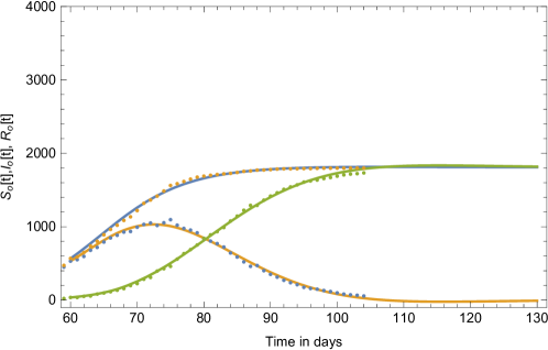
Figure 3: The plots show the comparison between the solutions of the SIR  equations (continuous plots) and the infection data (point like plots)  for Iceland. The blue curve shows the confirmed cases, the red one gives the active ones and the green line define the recovered patients. Note that a solution of the SIR model with retardation closely approaches the observed data, for the properly chosen values of the four parameters $N,\beta,\gamma$ and $\tau.$ The non vanishing value of $\tau$ indicates that retardation plays a role in the description of the time evolution. process.

The general initial conditions defined in (33,34,35) were specified in the form

$$S(t_{o}) =\frac{S_{obs}(t_{o})}{k}=2840,$$ (58)

$$I(t) =\frac{I_{obs}(t)}{k}\text{ =}13.9888\exp(0.1731(t-39))\ \text{\ for all \ \ }t\leq t_{o},$$ (59)

$$R(t_{o}) =\frac{R_{obs}(t)}{k}=180,$$ (60)

where $S_{obs}(t_{o}),I_{obs}(t)$ and $R_{obs}(t_{o})$ are the data for the confirmed, active infected and recovered cases for Iceland in reference 9 at the day $t_{o}$ and before. The function defining the values of the infection curve at all the times before $t_{o}$, is obtained by fitting an exponential behavior to the data for $I_{obs}(t)$ in reference 9 , for the considered country. In this region of small number of infections, the exponential solutions are exact and gives an accurate fitting of the initial data.

After fixing the initial conditions, it remains the four free parameters $\ (n,\beta,\gamma,\tau)$ to be determined for defining the solution which better can match the data for all the future times $t\geq t_{o}.$ Then, for the already defined initial conditions we solved the set of equations (26,27,28) by attempting to approach the observed data for Iceland in the best way possible. The figure 3 shows the result of this process. The continuous curves represent the best exact solutions of the equations attained for three relevant quantities. The blue curve is the number of the observed confirmed, the red line shows the observed active cases and lastly, the green plot shows the observed recovered cases. The plotted quantities are the predictions for the ”observed” quantities are defined as

$$S_{o}(t) =k\text{ }S(t),$$ (61)

$$I_{o}(t) =k\text{ }I(t),$$ (62)

$$R_{o}(t) =k\text{ }R(t),$$ (63)

that is, the total numbers $S(t),$ $I(t)$ and $R$ after multiplied by $\ k=0.2.$ The curves of points show the corresponding data $S_{obs}(t),I_{obs}(t)$ and $R_{obs}(t)$ for Iceland obtained from reference 9 . The resulting optimal parameter values determining the shown approach of the solution to the data were:

$$N =9797,$$ (64)

$$\beta =172.5\times 10^{-7},$$ (65)

$$\gamma =0.063,$$ (66)

$$\tau =8.$$ (67)

The figure 3 clearly indicates that a solution of a SIR model exists which reproduces in a satisfactory form the observed epidemic data curves for Iceland. It should be noted that it was attempted to match the observed and solved time evolution by avoiding to introduce retardation effects, that is fixing $\tau=0.$ However, it turned out to be impossible for us to attain a similar likelihood as the one shown in figure 3. Only after choosing a non vanishing retardation value $\tau$, it became possible to match the two behaviors as in the figure 3.

V.2 New Zealand

The behavior of the epidemics for New Zealand was very similar to the one of Iceland. After equally getting the initial data from reference 9 and choosing the time for the initial condition to be

$$t_{o}=64,$$ (68)

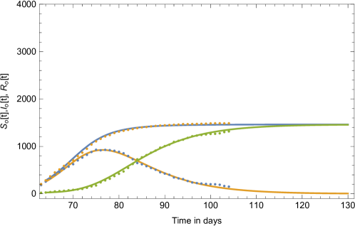
Figure 4: The figure presents the confirmed, active and recovered cases as continuous blue, red and green plots, respectively. It can be noted that in this case of New Zealand the infection data (point like plots) the solution of the SIR model with retardation, also well resembles the observed data, when proper values of the four parameters $N,\beta,\gamma$ and $\tau$ are chosen. Observe that retardation is also important in describing the time evolution.

the initial conditions (33,34,35) were written for this country as follows

$$S(t_{o}) =\frac{S_{obs}(t_{o})}{k}=1415,$$ (69)

$$I(t) =\frac{I_{obs}(t)}{k}\text{ =}0.0885\exp(0.3187(t-39))\ \text{\ for all \ \ }t\leq t_{o},$$ (70)

$$R(t_{o}) =\frac{R_{obs}(t)}{k}=135,$$ (71)

where $S_{obs}(t_{o}),I_{obs}(t_{o})$ and $R_{obs}(t_{o})$ are again the data for the confirmed, active infected and recovered cases for New Zealand found in reference 9 for the time $t_{o}$ and before. As for the previous case the function defining the values of the infection curve at all times before $t_{o}$, is evaluated after fitting an exponential behavior to the data for $I_{obs}(t)$ in reference 9 .

Then, in a closely form as in the previous subsection we solved the set of equations (26,27,28) successively in order to approach the observed data in this case for New Zealand. The figure 4 shows the outcome. As before, the continuous curves represent the best exact solutions of the equations attained for the three relevant quantities. The blue curve again is the number of the observed confirmed, the red one depicts the observed active cases and the green curve illustrates the observed recovered cases: defined as before by

$$S_{o}(t) =k\text{ }S(t),$$ (72)

$$I_{o}(t) =k\text{ }I(t),$$ (73)

$$R_{o}(t) =k\text{ }R(t).$$ (74)

The curves of points again show the corresponding data $S_{obs}(t),I_{obs}(t)$ and $R_{obs}(t)$ in this case for New Zealand, also obtained from reference 9 . The resulting parameter values for which maximal likelihood was attained took the values

$$N =7424,$$ (75)

$$\beta =360.5\times 10^{-7},$$ (76)

$$\gamma =0.063,$$ (77)

$$\tau =5.5.$$ (78)

The figure 4 again evidence that a solutions of a SIR model appropriately reproduce the form the data curves also in this case for New Zealand.

It also was attempted to match the observed and evaluated time evolution without considering retardation ($\tau=0$). As before, it was not possible to fit the data as closely as in figure 4. A retardation value $\tau=5.5$ days was required to adjust the curves.

V.3 South Korea

The initial conditions for the study of the South Korea epidemic data were fixed at

$$t_{o}=39,$$ (79)

and the chosen starting and retarded values for the total $S,$ $I$ and $R$ defined as follows

$$S(t_{o}) =\frac{S_{obs}(t_{o})}{k}=53825,$$ (80)

$$I(t) =\frac{15.1135\exp(0.2803(t-20))\text{\ }}{k}\text{for all \ \ }t\leq t_{o},$$ (81)

$$R(t_{o}) =\frac{R_{obs}(t)}{k}=46530.$$ (82)

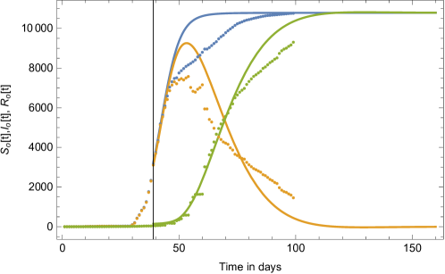
Figure 5: The figure expose the results for the infection data corresponding to South Korea. As before, the blue, red and green continuous curves show the solutions for the number of the observed confirmed $S_{o}$, active $I_{o}$ and recovered $R_{o}$ cases, respectively. Up to the day 43 (near 4 March 2020) the solutions again well match the observed data. After this time the continuous curves deviate from the observations. However, precisely the March 4, South Korea appreciably increased the isolation measures, breaking in this way the stationary character of the imposed isolation rules. Thus, the figure, also confirm the conclusion about that a modified SIR models describe the infections under stationary isolation rules.

After following exactly the same steps as in the discussion in the previous two subsections, the values of the four free parameters in order to approach the data as shown in figure 5, were found in the form

$$N =398305,$$ (83)

$$\beta =47.1645\times 10^{-7},$$ (84)

$$\gamma =0.035,$$ (85)

$$\tau =12.$$ (86)

The analysis brought an additional new element to the former discussions in previous subsections. As shown in figure 5 the three solutions of the equations, are shown by continuous curves. The blue one is the observed number of confirmed cases, the red one corresponds to the observed number of active cases and lastly, the green one presents the number of recovered cases.

However, near the day 43 (4 March 2020) it can be noted that the curve for the solution of the SIR model starts deviating from the observed data. This observation led us to search in the literature information about how were implemented the isolation measures in South Korea. Surprisingly, it was found that precisely the 4 March, the country had defined a drastic increase in the rigor of such measures. Therefore, the mentioned deviation of the solutions from the observed data, can be interpreted as produced by the breaking of the stationary character of the confinement rules, which were established up to such a moment. Thus, the example of South Korea can be also supporting the main conclusions of the present work.

V.4 Cuba

In the case of Cuba, in which tight isolation measures were also taken, they were established nearly the date 03.24.20, that is, at the time measured in days from the 01.22.20

$$t_{o}=63.$$ (87)

The initial conditions chosen for the equations (26,27,28) at that moment were

$$S(t_{o}) =\frac{S_{obs}(t_{o})}{k}=240,$$ (88)

$$I(t) =\frac{I_{obs}(t)}{k}\text{ =}\frac{0.0303054\exp(0.305211(t-39))}{k}\text{\ for all \ \ }t\leq t_{o},$$ (89)

$$R(t_{o}) =\frac{R_{obs}(t)}{k}=5\text{ }.$$ (90)

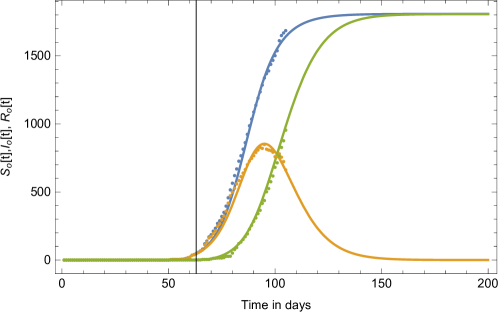
Figure 6: The blue, red and green continuous curves present the Cuba’s solutions for the observed confirmed $S_{o}$, active $I_{o}$ and recovered $R_{o}$ cases, respectively. The stationary character of the isolation measures sustained in the country, is consistent with appreciable degree of matching between the solution and the observations shown by the figure.

As in the previous subsections, the function $I_{obs}(t)$ defines the number of observed infections for all times before$\ t_{o}$, information which is needed to determine the solution of the retarded equations. In the present case it was evaluated in a continuous way by interpolating the observed discrete values of the infection curve before the day $63$. Reiterating the process of determining the best parameters for which the solution of the SIR equations with retardation shows a close likelihood with the data, the attained parameter values resulted in

$$N =9775,$$ (91)

$$\beta =170.9\times 10^{-7},$$ (92)

$$\gamma =0.06,$$ (93)

$$\tau =6.5\text{ }.$$ (94)

The figure 6 illustrates the observed confirmed cases $S_{o}$ $(t)=k$ $S(t)$ with the blue curve, the active ones $I_{o}(t)=k$ $I(t)$  with the red one and the recovered cases $R_{o}(t)=k$ $R(t)$ are shown in the green curve. The results further support that the solutions of a modified SIR model well describe the dynamics of the covid-19 epidemics under stationary isolation measures.

V.5 United States

We also have considered the case of United States. This country can not be considered as one in which rigorous and stationary in time isolation conditions had been implemented to stop the epidemic.

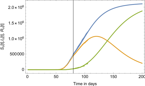
Figure 7: The figure shows the solutions of the SIR model with retardation for the case of United States. Again the continuous curves present the confirmed $S_{o}$, active $I_{o}$ and recovered $R_{o}$ cases respectively. For US the stationary character of the isolation measures can not be assured. However, due to the strong character of the infection in this country the SIR solutions were compared with the observed data, in order to estimate important quantities as the date and amount of infected cases in the peak of the infection curve. The figure shows a reasonable degree of matching of a SIR solution with the observed data. The resulting estimation for the date of the peak is May 20, 2020 with a maximum of nearly $1.064$ $\times 10^{6}$ observed active cases.

However, we consider the application of the model by two main reasons: the country’s data show a somewhat regular evolution which seemingly could be approximately approached by a solution of the SIR equations. In second place, due to the strong behavior of the epidemic in the country, it looks helpful to explore the predictions of the model in order to estimate the date for the occurrence and number of infected cases of the maximum of the infected curve.

The initial time for searching a solution of the equations (26,27,28) was

$$t_{o}=80,$$ (95)

and the initial (for $S$ and $R$ ) and retarded data (for $I$) in this case were

$$S(t_{o}) =\frac{S_{obs}(t_{o})}{k}=2.48268\times 10^{6},$$ (96)

$$I(t) =\frac{f_{int}(t)}{k}\text{ for all \ }t\leq t_{o},$$ (97)

$$R(t_{o}) =\frac{R_{obs}(t_{o})}{k}=143950,$$ (98)

in which $\frac{S_{obs}(t_{o})}{k}$ and $\frac{R_{obs}(t_{o})}{k}$ are the number of observed infected and recovered cases at the day $t_{o}=80$ after divided by $k,$ in order to define the total number of cases at this time. The function $f_{int}(t)$ defines the retarded data for the number of active cases as a continuous interpolation function of the set of discrete data points $I_{obs}$ for the observed active cases. The number of observed three types of cases were taken from reference 9 . As in all the previous cases, the search for solutions closely representing the data furnished the following set of parameters

$$N =1.1358\times 10^{7},$$ (99)

$$\beta =0.056\text{ }\times\text{\ }10^{-7},$$ (100)

$$\gamma =0.022,$$ (101)

$$\tau =16.$$ (102)

The figure 7 shows the solution (continuous lines) in comparison with the data (point like curves). As always, the plots correspond to the observed number of confirmed (in blue line), infected (red line) and recovered (green line) cases $S_{o}(t),$ $I_{o}(t)$ and $R_{o}(t)$, which as before, are the total numbers (which the solution furnishes) after multiplied by $k$, that is

$$S_{o}(t) =k\text{ }S(t),$$ (103)

$$I_{o}(t) =k\text{ }I(t),$$ (104)

$$R_{o}(t) =k\text{ }R(t).$$ (105)

The figure 7 shows that a definite solution of a modified SIR model reasonably match the observed data for the three quantities. Only the resulting value for the recovery parameter $\gamma$ took a slightly small value nearly a half of the values for the previously discussed countries. In addition, the probably lack of stationary character of the isolation measures, makes clear that assuming that they are stationary along the country is a very strong assumption. Thus, the maximum of the active cases and the date at which it appears can be only taken as a estimate of those quantities. The predicted values are

$$t_{\max}(US) =120\equiv\text{ May 20,}$$

$$I_{\max} =1.064\text{ \ }10^{6}.$$

V.6 Mexico

Finally, we discuss the case of Mexico. In similar way as USA, in Mexico rigorous and stationary in time isolation conditions had not been imposed.

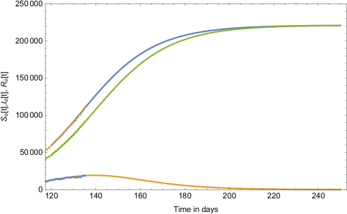
Figure 8: The figure shows the solutions of the SIR model with retardation for the case of Mexico. As before, the continuous curves present the confirmed $S_{o}$, active $I_{o}$ and recovered $R_{o}$ cases respectively. For Mexico, also, the stationary character of the isolation measures can not be assured. However, due to the large population of the country and the irregularities in the evolution of the infection the SIR solutions were compared with the observed data, seeking to estimate important quantities as the date and amount of infected cases in the peak of the infection curve. In spite of the above remarks, the figure shows a reasonable degree of matching of a SIR solution with the observed data. The resulting estimation for the date of the peak is June 10, 2020 with a maximum of nearly $20,000$ observed active cases.

As for the case of USA we consider the application of the model because the country is a large one and the infection data had showed an irregular evolution.

The initial time for searching a solution of the equations (26,27,28) was

$$t_{o}=120,$$ (106)

and the initial (for $S$ and $R$ ) and retarded data (for $I$) in this case were

$$S(t_{o}) =\frac{S_{obs}(t_{o})}{k}=297835,$$ (107)

$$I(t) =\frac{f_{int}(t)}{k}\text{ for all \ }t\leq t_{o},$$ (108)

$$R(t_{o}) =\frac{R_{obs}(t_{o})}{k}=233310,$$ (109)

in which as in the previous subsections $\frac{S_{obs}(t_{o})}{k}$ and $\frac{R_{obs}(t_{o})}{k}$ are the number of observed infected and recovered cases at the day $t_{o}=80$ after divided by $k,$ in order to define the total number of cases at this time. The function $f_{int}(t)$ defines the retarded data for the number of active cases as a continuous interpolation function of the set of discrete data points $I_{obs}$ for the observed active cases. Again, the number of observed three types of cases were taken from reference 9 . For Mexico the search for solutions closely representing the data gave the following results

$$N =220,000,$$ (110)

$$\beta =1.20\times\text{\ }10^{-7},$$ (111)

$$\gamma =0.18,$$ (112)

$$\tau =0.$$ (113)

Figure 8 exhibits the solution (continuous lines) in comparison with the data (point like curves). The plots correspond to the observed number of confirmed (in blue line), infected (red line) and recovered (green line) cases $S_{o}(t),$ $I_{o}(t)$ and $R_{o}(t)$. These quantities, as before, are the total numbers (which the solution furnishes) after multiplied by $k$, that is

$$S_{o}(t) =k\text{ }S(t),$$ (114)

$$I_{o}(t) =k\text{ }I(t),$$ (115)

$$R_{o}(t) =k\text{ }R(t).$$ (116)

The figure 8 indicates that a solution of a modified SIR model reasonably match the observed data for the three quantities. It is of interest to note that the recovery parameter $\gamma$ has a slightly high value, being larger than the ones for the all previously discussed countries. It is curious that the number of recovered cases in Mexico is from the start of the epidemic, larger that the number of active cases. This property is seemingly compatible with the observed high value of the recovery parameter.

Like for U.S.A., the probably lack of stationary character of the isolation measures, suggests doubts about the validity of a SIR model with constant parameters, as the one applied. Thus, the maximum of the active cases and the date at which it appears can be only taken as a rough estimate of those quantities. The resulting values were

$$t_{\max}(Mexico) =140\equiv\text{ June 10,}$$

$$I_{\max} =19,300.$$

Conclusions

It is argued that under stationary in time isolation measures, the SIR equations should be valid for the description of the epidemics, after disregarding statistical fluctuations. The resulting modified SIR equations have a reduced population parameter $N$ and a constant contagion rate $\beta$. The relevance of the retardation for properly describing the observed infection curves is also identified. A modified SIR model including retardation is introduced and applied to describe the infection data for various countries. The results properly confirm the idea about that when the isolation measures are stationary in time, the SIR equations solutions properly describe the observed confirmed, infection and recovering cases daily data.

The results also show that the solutions of the effective SIR with adjustable parameters (including the population number) when the total number of infected cases is very much smaller than the population, also exactly solve the SIR equations for the whole population. This conclusion allows to solve an existing challenging problem about how to define the required time dependence of the contagion parameter when the SIR model is decided to be applied to the whole population 14 ; 15 ; 16 ; 17 ; 18 ; 19 . The time dependence to be imposed for describing population under stationary isolation regimes is here exactly determined thanks to the also known exact solution of the SIR model harko .

The discussion also allows to propose here two procedures for predicting the infection curves, after observing the data, up to a time $T$ before the arrival to a maximum number of infected cases. A first possible method, is to minimize the square deviation between the solution and the observed data for all times before the moment $T$. The expectation is that this minimization process could be able to define the four relevant parameters of the SIR model with sufficiently small error, to efficiently predict the future evolution of the infection, after the chosen time $T$. Another way is to solve the linear equations for the SIR for the whole population employing the derived formula for the time dependent contagion parameter $\beta(t).$ In this case, an analogous to the above described method of minimizing the square deviation can be also employed.

Finally, the effective SIR model is applied to various countries in which proper isolation measures had been taken in combating the epidemic. The results for them appropriately match the observations after properly accounting for the delay between recovery and infection processes. There are also discussed two countries in which isolation measures can not be assured that had been constantly in time adopted: USA and Mexico. However, the results for the observations for a not too large time interval can be also reasonably reproduced.

References

- (1) The SARS-CoV-2 in Mexico: analysis of plausible scenarios of behavioral change and outbreak containment, M. A. Acuña-Zegarra et al. https://www.medrxiv.org, 2020.
- (2) An updated estimation of the risk of transmision of the novelcoronavirus (2019-nCov), B. Tang, N. L. Bragazzi, Q. Li, S. Tang, Y Xiao and J. Wu. Infectious Diseases Modelling 5, 248-255, 2020.
- (3) Modelo de infectados para el Edo. de Guanajuato COVID-19 , J. Barranco y A. Bernal, unpublished.
-
(4)
Como usé las matemáticas para predecir
COVID-19 en el estado de Guanajuato, México, Lisa Shiller.
https://www.lisashiller.com/blog-1/cmo-us-las-matemticas-para- predecir-covid-19-en-el-estado-de-guanajuato-mxico. - (5) Substantial undocumented infection facilitates the rapid dissemination of novel coronavirus (SARS-CoV2), R. Li, S. Pei, B. Chen, Y. Song,T. Zhang, W. Yang and J. Shaman, Science 368, 489-493, 2020.
-
(6)
Public Health responses to COVID-19 outbreaks on cruise ships
euro Worldwide, February href euro, March 2020, Moriarty et al.
https://www.cdc.gov/mmwr/volumes/69/wr/mm6912e3.htm - (7) A SIR epidemic model with time delay and general nonlinear incidence rate, M. Li and X. Liu, Hindawi Publishing Corporation, Abstract and Applied Analysis Vol. 2014, Article ID 131257.
- (8) Infectious disease models with time-varying parameters and general nonlinear incidence rate, X. Liu and P. Stechlinski, Applied Mathematical Modelling 36, 1974-1994, 2012.
- (9) Website: https://data.humdata.org/dataset/novel-coronavirus-2019-ncov-cases
-
(10)
Website:
https://medium.com/data-for-science/epidemic-modeling-101-or-
why-your-covid19-exponential-fits-are-wrong-97aa50c55f8 - (11) Website: https://www.worldometer.info.
- (12) Modelos SIR modificados para la evolucion del COVID19, N. G. Cabo-Bizet and A. Cabo Montes de Oca. Submitted and accepted to be published in Revista Cubana de Matematicas in 2020. arXiv:2004.11352v1 [q-bio.PE] 23 April 2020.
- (13) Estimating the number of infections and the impact of non- pharmaceutical interventions on COVID-19 in 11 European countries, S. Flaxman, S. Mishra and A. Gandy and S- Bhatt, Nature doi.org./10.1038/s41586-020-24025-7, 2020.
- (14) Das mysterium um die ansteckungsrate, Katherine Rydlink, Spiegel Online, 17 April 2020, https://www.spiegel.de
- (15) Time-dependent and time-independent SIR models applied to the COVID-19 outbreak in Argentina, Brazil, Colombia, Mexico and South Africa, N. G. Cabo-Bizet and D. Mayorga Pena, arXiv:2006.12479v1 [q-bio.PE], 2020.
- (16) Exact analytical solutions of the Susceptible-Infected-Recovered (SIR) epidemic model and of the SIR model with equal death and birth rates, T. Harko, F. S. N. Lobo and M. K. Mak, Applied Mathematics and Computation 236, 184-194, 2014.
- (17) Modeling the Transmission of Middle East Respiratory Syndrome CoronaVirus in the Republic of KoreaZ-Q Xia, J. Zhang, Y-K. Xue, G-Q. Sun, Z. Jin, PLoSONE 10,(12): e0144778, 2015.
- (18) Predicting the evolution of SARS-COVID-2 in Portugal using an adapted SIR model previously used in South Korea for MERS outbreak, P. Teles, arXiv:2003.10047v2 [q-bio.PE] 9 Apr 2020.
- (19) Estimation of timevarying reproduction numbers underlying epidemiological processes: A new statistical tool for the COVID-19 pandemic, H. G. Hong and Y. Li, PLoS ONE 15,(7): e0236464, 2020.
- (20) A Time-dependent SIR model for COVID-19 with Undetectable Infected Persons, Yi-Cheng Chen, Ping-En Luy, Cheng-Shang Changz and Tzu-Hsuan Liux, arXiv:2003.00122v6 [q-bio.PE] 28 Apr 2020.
- (21) SIR model with time dependent infectivity parameter: approximating the epidemic attractor and the importance of the initial phase, S. Boatto, C. Bonnet, B. Cazelles and F. Mazenc, hal-01677886, 2018.
- (22) An epidemiological forecast model and software assessing interventions on COVID-19 epidemic in China, L. Wang, Y. Zhou, J. He, B. Zhu, F. Wang, L. Tang, M. Eisenberg and P. X. K. Song, medRxiv preprint doi: https://doi.org/10.1101/2020.02.29.20029421, posted March 3, 2020.