On the Effect of Selfie Beautification Filters on Face Detection and Recognition

Abstract

Beautification and augmented reality filters are very popular in applications that use selfie images. However, they can distort or modify biometric features, severely affecting the capability of recognizing individuals’ identity or even detecting the face. Accordingly, we address the effect of such filters on the accuracy of automated face detection and recognition. The social media image filters studied either modify the image contrast or illumination or occlude parts of the face. We observe that the effect of some of these filters is harmful both to face detection and identity recognition, specially if they obfuscate the eye or (to a lesser extent) the nose. To counteract such effect, we develop a method to reverse the applied manipulation with a modified version of the U-NET segmentation network. This is observed to contribute to a better face detection and recognition accuracy. From a recognition perspective, we employ distance measures and trained machine learning algorithms applied to features extracted using several CNN backbones. We also evaluate if incorporating filtered images to the training set of machine learning approaches are beneficial. Our results show good recognition when filters do not occlude important landmarks, specially the eyes. The combined effect of the proposed approaches also allow to mitigate the impact produced by filters that occlude parts of the face.

Pattern Recognition Letters

Authorship Confirmation

Please save a copy of this file, complete and upload as the “Confirmation of Authorship” file.

As corresponding author I, Fernando Alonso-Fernandez, hereby confirm on behalf of all authors that:

1. This manuscript, or a large part of it, has not been published, was not, and is not being submitted to any other journal.

2. If presented at or submitted to or published at a conference(s), the conference(s) is (are) identified and substantial justification for re-publication is presented below. A copy of conference paper(s) is(are) uploaded with the manuscript.

3. If the manuscript appears as a preprint anywhere on the web, e.g. arXiv, etc., it is identified below. The preprint should include a statement that the paper is under consideration at Pattern Recognition Letters.

4. All text and graphics, except for those marked with sources, are original works of the authors, and all necessary permissions for publication were secured prior to submission of the manuscript.

5. All authors each made a significant contribution to the research reported and have read and approved the submitted manuscript.

Signature                                                             Date                                   

 

List any pre-prints:

 

Relevant Conference publication(s) (submitted, accepted, or published):

Justification for re-publication:

Graphical Abstract (Optional)

To create your abstract, please type over the instructions in the template box below. Fonts or abstract dimensions should not be changed or altered.

On the Effect of Selfie Beautification Filters on Face Detection and Recognition Pontus Hedman, Vasilios Skepetzis, Kevin Hernandez-Diaz, Josef Bigun, Fernando Alonso-Fernandez This is the dummy text for graphical abstract.

Research Highlights (Required)

To create your highlights, please type the highlights against each \item command.

It should be short collection of bullet points that convey the core findings of the article. It should include 3 to 5 bullet points (maximum 85 characters, including spaces, per bullet point.)
1. We summarise works in image digital manipulation with the purpose of facial beautification 2. We study the impact of enhancement and Augmented Reality filters on face detection and recognition 3. We develop a method to reverse the applied manipulations that entail eye obfuscation 4. We study if training the recognition system with manipulated images helps to increase accuracy

1 Introduction

Selfie images captured with smartphones enjoy huge popularity and acceptability, and social media platforms centered around sharing such images offer several filters to ”beautify” them before uploading. Filtered images are more likely to be viewed and commented, achieving a higher engagement (Bakhshi et al., 2021). Selfies are also increasingly used in security applications since mobiles have become data hubs used for all type of transactions (Rattani et al., 2019). Even video conference applications, which have boomed during the pandemic, include beautification or augmented reality filters too.

A challenge posed by such filters is that facial features may be distorted or concealed. Given their low cost and instant availability, they are a commodity used daily by many, not necessarily with the aim of compromising face recognition systems. However, the capability of recognizing individuals may be affected, and even the possibility of detecting the face itself before any recognition can take place. This is crucial for example in crime investigation on social media (Powell and Haynes, 2020), where automatic pre-analysis is necessary given the magnitude of information posted or stored in confiscated devices (Hassan, 2019). There are multiple examples of crimes captured on mobiles (Berman and Hawkins, 2017; Pagones, 2021), with the most striking lately being the use of posted videos of the US Capitol to identify rioters (Morrison, 2021).

There is, therefore, interest to study the consequences of different levels of image manipulation and concealment of facial parts due to these ”beautification” filters. It would be also of interest to evaluate methods that remove the filter’s effect to avoid a decrease in face detection and recognition performance. The purpose and contributions of this work are therefore multi-fold. We first summarize related works in image digital manipulation, in particular with the purpose of facial beautification. Then, we study the impact of image enhancement and Augmented Reality (AR) filters both on the detection of filtered faces and on the recognition of individuals. To counteract the effect of such filters, we develop a method to reverse some of the applied manipulations. We focus on reversing modifications to the eye region, since these are observed to have the biggest impact on face detection or recognition. Another strategy that we propose is the use of manipulated images to train the identity recognition system, which is also observed to increase accuracy when such manipulations are present in test images as well.

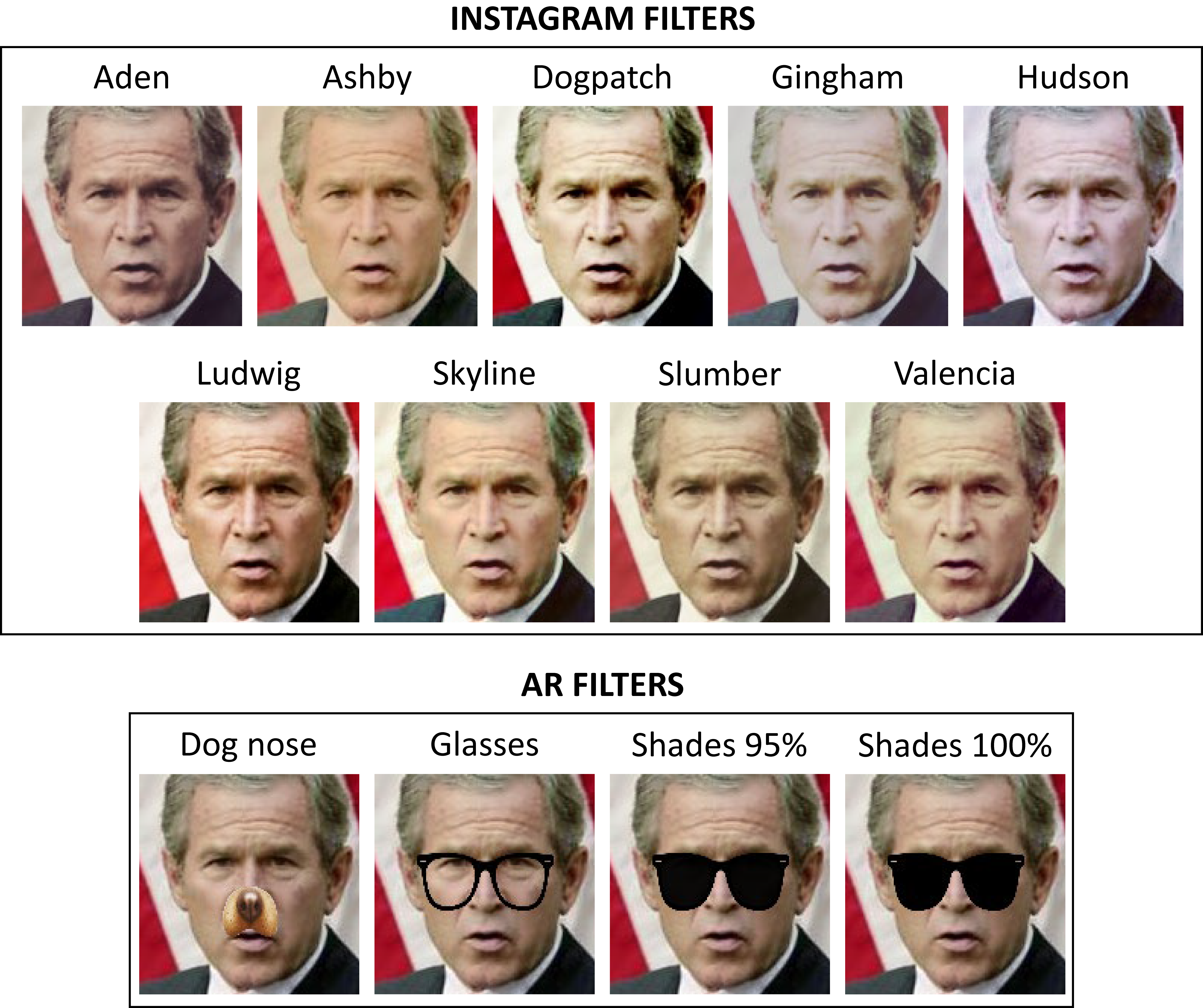
Fig. 1: Examples of the filters applied.

2 Related Works

Facial manipulation can be done in the physical or digital domain. Physical manipulation can be achieved for example via make-up or surgery, while digital manipulation or retouching is via software (Rathgeb et al., 2019). Physical manipulation can be permanent (surgery) or non-permanent (make-up). Make-up can be quickly induced, so the same person may appear different even after a short period. Also, given the wide acceptance of cosmetics, it may also appear in enrolment data. Digital retouching allows similar modifications than surgery or cosmetics, but in the digital domain, as well as other changes such as re-positioning or resizing facial landmarks. A common aim of these modifications is to improve attractiveness (beautification). Of course, it is also possible that someone pretends to look like somebody else to gain illegitimate access, or to hide the own identity to avoid recognition (Ramachandra and Busch, 2017; Scherhag et al., 2019). Another manipulation is the use of facial masks, either surgical due to the current pandemic (Damer et al., 2020), or artificial as used in Presentation Attacks (Ramachandra and Busch, 2017). However, this is out of the scope of this paper, since they are not oriented towards beautification.

Some works focus on detecting retouched images. The methods proposed include Supervised Restricted Boltzmann Machine (SRBM) (Bharati et al., 2016), semi-supervised autoencoders (Bharati et al., 2017), or Convolutional Neural Networks (CNN) (Jain et al., 2018). They also present new databases such as the ND-IIITD Retouched Faces Database (Bharati et al., 2016) or the MDRF Multi-Demographic Retouched Faces (Bharati et al., 2017), generated with paid and free applications that provide for example skin smoothing, face slimming, eye/lip color change, eye/teeth brightening, etc. Authors of the MDRF database also analyze the impact of gender or ethnicity, showing that detection accuracy can vary greatly with the demographics. The work (Jain et al., 2018) also analyzes the detection of GAN-altered images. All these approaches consider the use of a single image (the retouched one). In contrast, Rathgeb et al. (2020) proposes a differential approach where the unaltered image is also available, something which, according to the authors, is plausible in some scenarios (e.g. border control). They use texture and deep features with images of the FERET and FRGCv2 datasets. Retouching is done with free applications from the Google PlayStore, arguing that free applications are more likely to be used by consumers.

Another set of works analyze the impact of manipulated images on the recognition performance. In (Dantcheva et al., 2012), they gather two databases of Caucasian females with makeup. One is from before/after YouTube tutorials mostly affecting the ocular area, and the other is by modification of FRGC images with lipstick, eye makeup or full makeup. The study employs Gabor features, LBP and a commercial system, showing an increase in error when testing against makeup pictures. They also found that applying LBP to Gabor filtered images (as opposed to the original image) partly compensates the effect. In (Ferrara et al., 2013), alterations such as barrel distortion or aspect ratio change are studied. They also simulate surgery digitally, such as injectables, wrinkle removal, lip augmentation, etc. They employ the AR face database, with two commercial and a SIFT algorithm, concluding that the systems can overcome limited alterations, but they stumble on heavy manipulations. Digital retouching is studied in (Bharati et al., 2016) with the ND-IIITD database. They use a commercial system and OpenBR, an open source face engine, finding that the performance is considerably degraded when testing against retouched images. Image retouching is also examined by Rathgeb et al. (2020) with a commercial system and the open-source ArcFace, showing its negative impact as well.

3 Materials and Methods

3.1 Beautification Filters

We focus on two manipulations: image enhancement and Augmented Reality (AR). AR filters in particular have not been addressed in the literature. For enhancement, we use the 9 most popular selfie Instagram filters (Canva, 2020), which mostly change contrast and lighting (Figure 1, top). The ranking is based on the images with each filter and the hashtag “#selfie”. Since the Instagram API does not allow to process a large amount of data, the filters are recreated with a four-layer neural network (Hoppe, 2021). Regarding AR filters, they obfuscate face parts that can be critical for recognition (Figure 1, bottom). Such filters are very popular in social media (e.g. Snapchat) and even in video conference platforms. We apply: Dog nose, Transparent glasses, Sunglasses-slight transparency, and Sunglasses-no transparency. These are merged with the face by using the landmarks (Figure 2(b)) given by (Geitgey, 2018).

(a) Original

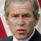
(b) Landmarks

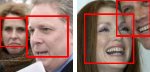
(c) Multiple faces

Fig. 2: Example of: (a), (b) detected landmarks, (c) multiple faces detected.

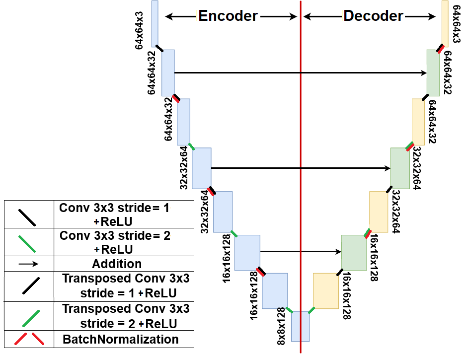
Fig. 3: U-NET model employed. The blue rectangles are convolutions (compression), the yellow are transpose convolutions (expansion), and the green symbolizes the addition of blue and yellow through the add operation.

3.2 Image Reconstruction with U-NET

We use a modified version of the U-NET network. Originally presented for image segmentation (Ronneberger et al., 2015), it outperformed more complex networks in accuracy and speed while requiring less training data. It has a compression or encoding path with convolutions and max-pooling, followed by decompression or decoding path with up-convolutions. This gives the network a U-shape (Figure 3). Residual links connect maps of the encoding and decoding paths, with channels concatenated, allowing the model to focus on the parts of the image that change. The original network has been modified, since the task is different. Inspired by Springenberg et al. (2015), max-pooling and up-convolutions are changed to strided convolutions/transposed convolutions. Also, map concatenation in residual links is changed by addition to halve the number of channels. With this, we expect to still retain changes of image patches while counteracting over-fitting.

3.3 Databases

We use the version aligned by funneling (Huang et al., 2012) of Labeled Faces in the Wild (LFW) (Huang et al., 2007). It has 13,233 images of 5,749 celebrities from the web with large variations in pose, light, expression, etc. To ensure a sufficient amount of images per person, we remove people with less than 10 images, resulting in 158 individuals and 4,324 images. Five datasets are then created by applying the Instagram and AR filters of Section 3.1. The Instagram dataset is created by applying one filter randomly to each unfiltered image. Additionally, images with sunglasses are processed with the U-NET method of Section 3.2, giving two more datasets of reconstructed images. This results in 8 different datasets, listed in Table 1.

U-NET is trained to reconstruct the filters shades_leak and shades_no_leak (Figure 1, bottom right) with the CelebA dataset ($202,599$ pictures of $10,177$ people) (Liu et al., 2015). We use a batch size of 64, with Adam as optimizer and the MSE between the output and the target (unfiltered) images as loss. CelebA is not used for biometric recognition experiments, allowing to test the generalization ability of the U-NET model on unseen data.

3.4 Face Detection and Feature Extraction Algorithms

The 8 datasets are further encoded into a feature vector that will be used for biometric authentication. First, faces are detected with the face_location function of (Geitgey, 2018), which is based on the dlib Python library. The detector used is the more accurate CNN, rather than the default HOG model. The CNN detector is trained with 7213 face images gathered from publicly available datasets including ImageNet, AFLW, Pascal VOC, VGG, WIDER, and face scrub. If more than one face or no face is found, the image is discarded (e.g. Figure 2(c)), and it is no further considered for feature extraction or recognition experiments. Our baseline feature extractor is a ResNet34 model of 29 convolutional layers with the filters per layer reduced by half (King, 2017), pre-trained from scratch for face recognition using $\sim$3M faces of 7485 identities from the VGG dataset, the face scrub dataset, and other web-scraped images. It uses as input images of 64$\times$64, and produces a 128-dimensional vector (taken from the next-to-last layer). We also use two other available models, one based on the light SqueezeNet architecture (18 layers, 113$\times$113 input, 1000-dimensional vector) (Alonso-Fernandez et al., 2020) and a ResNet50 model (50 layers, 224$\times$224 input, 2048-dimensional vector) (Cao et al., 2018), both pre-trained for face recognition using $\sim$8.41M faces of $>$100K identities from the very large VGGFace2 and MS-Celeb-1M datasets. The latter two models are selected for comparison purposes with ResNet34 in order to assess the use of a light network suitable for mobile operation (SqueezeNet) and a much deeper ResNet50 network.

3.5 Face Identification and Verification Protocol

For identification, we carry out both closed- and open-set experiments. To find the closest subject of the database, we use both distance measures (Euclidean, Manhattan, and Cosine) and trained approaches (Support Vector Machines, SVMs (Cortes and Vapnik, 1995) and Extreme Gradient Boosting, XGBoost (Chen and Guestrin, 2016)). Since SVM is a binary classifier, we adopt a one-vs-all approach with multiple SVMs, taking the decision of the model that is the most confident. XGBoost is multi-class, using softmax with cross-entropy loss as objective. SVM is a widely employed classifier with good results in biometric authentication (Fierrez et al., 2018), and XGBoost has wide adoption in the industry, having obtained top rankings in recent machine learning challenges (DMLC, 2021). Before the experiments, feature vectors are scaled with min-max normalization, so each element is in the $[0,1]$ range.

To measure closed-set identification accuracy, we compute the False Negative Identification Rate (FNIR) (Tabassi et al., 2014), which is the fraction of mated searches (i.e. where there is an enrolled template for the search image) where the enrolled mate is not the closest subject of the database. As accuracy metric, we report the Genuine Accept Rate (GAR), computed as GAR=1-FNIR, which measures the fraction of mated searches where the enrolled template is in the top rank. Open-set identification accuracy is quantified by reporting the False Positive Identification rate (FPIR) and the False Negative Identification Rate (FNIR) (Tabassi et al., 2014). FPIR (also called False Accept Rate, FAR) is the fraction of non-mated searches (i.e. there is no enrolled template for the search image) where one or more enrolled identities are returned at or above an specified score threshold. To compute FNIR in open-set, one must consider if the mated search is not in the top rank or if its comparison score is below the threshold. FPIR and FNIR in open-set are obtained at different thresholds, after which we report the Detection Error Trade-off (DET), showing FPIR (FAR) against GAR.

For verification experiments, we use the same distance measures than before (Euclidean, Manhattan, Cosine). Accuracy is measured via False Rejection Rate (FRR) and False Acceptance Rate (FAR) at different distance thresholds (Wayman, 2009). Then, the DET curve is given, plotting FAR against FRR. As a single measure of accuracy, we also report the Equal Error Rate (EER), which is the error at the threshold where FAR=FRR.

Table 1: Summary description of the 8 datasets employed in the study. The numbers in brackets indicate the percentage of images of each dataset for which the face is correctly detected (see Section 3.4).

Name	Manipulation	Images
benchmark	Original images	4,276 (98.9%)
dog	Dog nose	4,229 (97.8%)
glasses	Transparent glasses	3,666 (84.8%)
instagram	Instagram filters	4,277 (98.9%)
shades_leak	Shades (95% opacity)	3,851 (89.1%)
shades_recon_leak	Reconstructed (95% op)	4,288 (99.2%)
shades_no_leak	Shades (100% opacity)	3,825 (88.5%)
shades_recon_no_leak	Reconstructed (100% op)	4,271 (98.8%)

Fig. 4: Example of images with AR glasses where the individual wears real glasses as well. In all these examples, the face detector fails.

(a) shades 95%

(b) shades 100%

Fig. 5: Examples of the reconstruction on the shades dataset. The left part of each sub-figure shows the first 10 pixel values of the images with shades (re-scaled to 0-255), while the right part shows the reconstructed image. Shades at 95% preserve some information, so a good reconstruction is still possible. Shades at 100%, on the other hand, destroys the pixels behind the shades.

Fig. 6: Class separation for the various datasets shown via t-SNE scatter plots after feature extraction with ResNet34 (perplexity=30).

Table 2: ResNet34: Identification Accuracy (closed set). The higher the value, the better.

	Distance measures			SVM			XGBoost
				Train=	Train=	Train=	Train=	Train=	Train=
Test Dataset	Eucl	Manh	Cosine	Bench.	Filter	All	Bench.	Filter	All
benchmark	0.930	0.921	0.925	0.993	N/A	0.999 (+0.006)	0.993	N/A	1.000 (+0.007)
dog	0.562	0.543	0.539	0.921	0.966 (+0.045)	0.982 (+0.061)	0.917	0.974 (+0.057)	0.986 (+0.069)
glasses	0.479	0.455	0.498	0.879	0.922 (+0.043)	0.967 (+0.088)	0.892	0.925 (+0.033)	0.967 (+0.075)
instagram	0.923	0.916	0.921	0.992	0.991 (-0.001)	0.998 (+0.006)	0.993	0.993 (+0.000)	1.000 (+0.007)
shades_leak	0.435	0.407	0.423	0.708	0.866 (+0.158)	0.964 (+0.256)	0.722	0.030 (-0.692)	0.964 (+0.242)
shades_recon_leak	0.663	0.639	0.655	0.885	0.946 (+0.061)	0.949 (+0.064)	0.881	0.932 (+0.051)	0.937 (+0.056)
shades_no_leak	0.386	0.365	0.379	0.672	0.854 (+0.182)	0.941 (+0.269)	0.663	0.009 (-0.654)	0.948 (+0.285)
shades_recon_no_leak	0.368	0.357	0.350	0.594	0.849 (+0.255)	0.827 (+0.233)	0.619	0.124 (-0.495)	0.825 (+0.206)
average	0.593	0.575	0.586	0.831	0.913 (+0,082)	0.953 (+0,122)	0.835	0.570 (-0,265)	0.953 (+0,118)

Table 3: ResNet34: Identification Accuracy (closed set), cross-filter experiments. The higher the value, the better. A graphical representation is given in Figure 7.

	SVM								XGBoost
	Test Dataset								Test Dataset
Train Dataset	bench- mark	dog	gla- sses	insta- gram	shades-				bench- mark	dog	gla- sses	insta- gram	shades-
					leak	recon- leak	no- leak	recon- no- leak					leak	recon- leak	no- leak	recon- no- leak
benchmark	0.993	0.921	0.879	0.992	0.708	0.885	0.672	0.594	0.993	0.917	0.892	0.993	0.722	0.881	0.663	0.619
dog	0.973	0.966	0.762	0.979	0.523	0.798	0.472	0.482	0.973	0.974	0.76	0.975	0.498	0.791	0.444	0.463
glasses	0.978	0.775	0.922	0.97	0.837	0.929	0.775	0.745	0.974	0.764	0.925	0.972	0.813	0.91	0.783	0.719
instagram	0.993	0.918	0.888	0.991	0.716	0.879	0.661	0.613	0.994	0.889	0.871	0.993	0.699	0.88	0.655	0.618
shades_leak	0.893	0.564	0.896	0.877	0.866	0.831	0.944	0.802	0.008	0.008	0.01	0.008	0.03	0.008	0.008	0.008
*_recon_leak	0.977	0.804	0.916	0.97	0.772	0.946	0.73	0.767	0.967	0.787	0.907	0.961	0.77	0.932	0.699	0.758
*_no_leak	0.863	0.512	0.858	0.855	0.957	0.802	0.854	0.805	0.008	0.008	0.01	0.008	0.009	0.008	0.009	0.008
*_recon_no_leak	0.838	0.53	0.79	0.82	0.839	0.857	0.817	0.849	0.006	0.006	0.005	0.006	0.005	0.006	0.004	0.124

4 Results and Discussion

Table 1 provides the number of images of each dataset for which a face is detected. Note that the detection accuracy varies across datasets, suggesting that the applied manipulations have different impact. The benchmark (unfiltered) dataset has a detection rate of $\sim$99%. The face is also detected successfully in case of Instagram filters, which can be expected since they mainly enhance contrast or lighting. Faces with a dog nose are also well detected, but occlusions in the eye region has a high impact. Indeed transparent glasses have the worst detection accuracy, even worse than shades. Only six failed images with transparent glasses contain more than one face, the rest being due to undetected face. One plausible reason after examination of the images is that several users wear real glasses as well (Figure 4). This very likely creates a disturbance to the detector that is not present in images with shades, where the real glasses of the user are obfuscated with 95% or 100% opacity. The synthetic nature of the glasses can also be a source of unpredictability for the detector, which has not “seen” this type of images beforehand. Such AR filters do not have a smooth blending with the source image. In the case of glasses, frame pixels are set directly to zero, and it may be that the transparent glasses constitute a higher source of perturbation than the shades (consider the transition to zero both at the outer and inner sides of the frame, which is completely unnatural and unexpected in a real face image). This is amplified even more if the user is wearing real glasses as well. In any case, face occlusion is a difficulty known to make detection systems to struggle (Zeng et al., 2021), with our results indicating that eye occlusion is more critical than nose occlusion. When the reconstruction network of Section 3.2 is applied to images with shades, detection accuracy is recovered to a higher extent ($\sim$99%), highlighting the benefits of the employed reconstruction. Figure 5 depicts the reconstruction of the two images with shades of Figure 1, showing a clear reconstruction of the majority of the eye area in the case of shades with 95% opacity. In the case of 100% opacity, the reconstruction is less successful, although sufficient to obtain a good detection accuracy.

Figure 6 details the class separation by t-SNE (van der Maaten and Hinton, 2008) of the features extracted with ResNet34. Only the five most frequent classes are colored due to colors’ limitation. For the benchmark (unmodified) and Instagram datasets, the clusters appear well separated, which suggests that class (identity) separation is possible. Clusters of the dog nose dataset are still separated, although closer and with higher intra-class variability. In the datasets with glasses, and specially with shades, the clusters appear much closer. It can be seen a parallelism between the t-SNE plots and the detection results of Table 1, in the sense that faces where the nose or eye appear obfuscated are more difficult to detect and to recognize.

We now report closed-set identification experiments in Table 2. With distance measures, the first original (unfiltered) image is used for enrolment, and identification attempts are done with filtered images. Comparatively, the Euclidean distance performs best, although just 1-2% better than the other metrics. The performance on the non-filtered benchmark and Instagram datasets are the highest, with minuscule differences between them ($\approx$92-93% for all distance measures). The dog dataset follows at $\approx$56%, and transparent glasses at $\approx$50%. The performance of shades_leak and shades_no_leak is poor, specially the latter one. After reconstruction, the shades_recon_leak dataset shows some performance recovery (66.3%). On the other hand, reconstruction with the non-leaking shades (100% opacity) does not contribute to any performance improvement.

To carry out closed-set identification experiments with trained methods, the datasets are split into 80% (training) and 20% (test). Training is done either with benchmark unfiltered images (“Train=Benchmark”), with filtered images of the corresponding test dataset (“Train=Filter”), or with images of all datasets together (“Train=All”). Identification tests are always done with filtered images. The splits between different datasets are the same to ensure comparability, achieved by use of scikit-learn function train$\_$test$\_$split (the hyper-parameter random$\_$state is initialized with the same value for each split). A first observation is that both trained methods behave similarly on the different datasets, at least in those that do not involve shades. With shades, SVM is comparatively better than XGBoost, at least when “Train=Filter” is applied. Also, both trained methods are widely benefited by “Train=Filter”, and specially by “Train=All”, which provides the best results overall. When training is done with all images, the performance of datasets not involving eye obfuscation reaches 98-100%, and even those involving shades or glasses are recovered to 94-97% in most cases. Indeed, shades_leak and shades_no_leak are boosted to the point of not needing reconstruction of the image before recognition. Combining the datasets have a beneficial effect, since the classifier is ’seeing´ images of the same individual with different perturbations, acting as a way of data augmentation. It should be considered though that the option “Train=All” has eight times more training data than the other options due to dataset pooling.

We also report in Table 3 cross-dataset experiments when the classifier is trained with one dataset (“Train=Filter”) and tested with another one. For better viewing, Figure 7 depicts the accuracy values (black=0%, white=100%), including the case “Train=All” in the first row for comparative purposes. It can be seen that when training does not include eye obfuscation (rows 2-5), testing with shades decreases performance significantly. Some performance recovery is achieved when testing with shades_recon_leak, since this reconstruction is observed to recover the eye region to a certain extent (Figure 5). Another phenomenon is the poor performance of XGBoost when training involves shades (black squares). Again, the only exception is shades_recon_leak, but in the other three cases, this classifier is unusable. Another interesting effect is that training with the dog dataset and testing with any glasses or shades dataset (or the opposite) produces the worst performance, apart from the XGBoost issue just mentioned (see the dark squares in row 3/column 2 of Figure 3). Dog and glasses/shades images are the most different images, in the sense that they have obfuscated different regions, so a significant portion of the face is different between training and test images. This makes that cross-filter classification struggles in identifying individuals. In such situation, it would be problematic if the wrong classifier is used. One way to cope with this effect, as we have seen above, is to train the classifiers with images from all datasets.

Next, we report open-set identification experiments in Figure 8. To do these experiments, we have set aside 58 random individuals as unseen people, and trained an SVM classifier with the remaining 100 individuals. The comparison score is the confidence measure given by the SVM. As before, the 100 individuals are split into 80% (training) and 20% (test). Training is done with images of all datasets together (“Train=All”), since it is the best performing option in the closed-set setting. The amount of mated searches where the enrolled mate is in the first position of the rank is 96.2% with ResNet34 (black curve, corresponding to the right side of the x-axis of Figure 8 where the threshold is sufficiently high to allow all mated searches to exceed it; other CNN backbones will be commented later). As we move left in the x-axis, the GAR reduces at the same time that the FAR reduces too. At FAR=10/1%, the obtained GAR is approximately 92/75% with ResNet34.

Finally, we report verification experiments (Table 4 and Figure 9) with the different distance measures. The first original (unfiltered) image is used for enrolment, and the remaining filtered images of the different datasets for verification attempts, both genuine (mated) and impostor (non-mated). As can be observed, the Euclidean distance performs best, although the other distances are less than 1% behind. The best EER is for benchmark and Instagram sets at $\approx$ 2%, with the rest (in descending order) at 7% (dog), 8.2% (glasses), 12.5% (shades_leak), and 14% (shades_no_leak). The EER for reconstructed shades_leak surpasses the dog results at 6%. Also, as before, reconstruction with the non-leaking shades (shades_recon_no_leak) does not show any improvement. The DET curves show a similar behaviour over the entire range of FAR and FRR values, with the relative performance of the systems becoming somehow closer to each other for low FAR values.

To conclude, we report the comparison of different CNN backbones under identification and verification (Figure 8 and Table 5). Experiments are carried out with the best options identified previously (identification: SVM classifier, “Train=All”; verification: cosine distance). One immediate observation is that the much deeper ResNet50 model surpasses the results obtained previously, being the best performing backbone. The closed-set identification accuracy is pushed towards higher values, including cases involving shades, which surpass 97% even without reconstruction (although both reconstructed and non-reconstructed images are present in the training set). The same can be said about verification, where the EER without any eye obfuscation is 1.6% (dog) or 0.7% (benchmark, instagram), and less than 3% with transparent glasses. Shades reconstruction also provides good results, with EER=2.2% (leak) and 5.3% (no_leak). The average EER of 2.9% with ResNet50 contrasts with the 8.4% obtained with ResNet34. As a side note, ResNet50 and SqueezeNet backbones are trained using much larger face datasets (recall Section 3.4), which may also contribute to a better face recognition performance. This can be appreciated by the fact that SqueezeNet in Table 5 has an identification accuracy that is just behind ResNet34, despite being a much lighter model. Indeed, the verification accuracy of SqueezeNet is better than ResNet34 in several cases, including those that entail eye obfuscation. In open set idenfication (Figure 8), we can again see the very good performance of ResNet50 (GAR 97/91% at FAR=10/1%), with SqueezeNet situated behind ResNet34.

Fig. 7: ResNet34: Identification Accuracy (closed set), cross-filter experiments. The higher the value, the better. The exact values are given in Table 7.

Fig. 8: Identification Accuracy (open set).

Table 4: ResNet34: Verification EER. The lower the value, the better.

Test Dataset	Eucl	Manh	Cosine
benchmark	0.019	0.020	0.020
dog	0.071	0.070	0.073
glasses	0.082	0.085	0.082
instagram	0.022	0.023	0.023
shades_leak	0.125	0.132	0.125
shades_recon_leak	0.062	0.067	0.060
shades_no_leak	0.140	0.147	0.144
shades_recon_no_leak	0.144	0.152	0.144
average	0.083	0.087	0.083

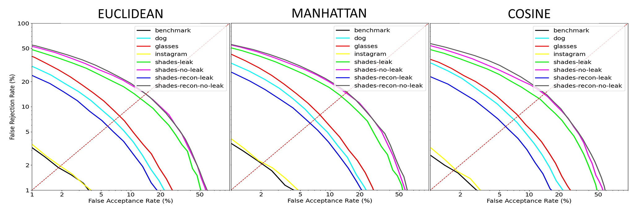
Fig. 9: ResNet34: Verification results (DET curves) using Euclidean, Manhattan and Cosine distance

Table 5: Comparison between different CNN backbones (R34=ResNet34, SQ=SqueezeNet, R50=ResNet50). Left: Identification Accuracy, closed set (the higher, the better). Right: Verification EER (the lower, the better).

	Closed set Identification (SVM, Train=All)			Verification (Cosine)
Test Dataset	R34	SQ	R50	R34	SQ	R50
benchmark	0.999	0.986	0.999	0.020	0.020	0.007
dog	0.982	0.966	0.992	0.073	0.035	0.016
glasses	0.967	0.917	0.985	0.082	0.085	0.028
instagram	0.998	0.985	0.999	0.023	0.020	0.007
shades_leak	0.964	0.911	0.977	0.125	0.098	0.048
*_recon_leak	0.949	0.953	0.990	0.060	0.054	0.022
*_no_leak	0.941	0.902	0.972	0.144	0.100	0.050
*_recon_no_leak	0.827	0.905	0.971	0.144	0.100	0.053
average	0.953	0.941	0.986	0.084	0.064	0.029

5 Conclusions

Social media platforms offer many different filters to beautify selfie images or to modify them by adding items like noses or glasses. We are thus interested in studying the effect of such filters on the accuracy of both face detection and recognition. The effect of some of the employed filters have been observed to be detrimental to both tasks, specially if the eye region is obfuscated. Thus, we explore methods to reverse the applied manipulations. Another strategy has been the use of filtered images for enrolment. In overall terms, by combining these two solutions, we manage to counteract the effect of the majority of the studied image modifications. The use of a deeper CNN backbone or a larger face dataset to pre-train the recognition backbones have been also seen as contributing factors. The latter becomes relevant for example under hardware limitations, since one of employed backbones (Alonso-Fernandez et al., 2020) is comparatively much shallower, but its performance is just behind deeper counterparts.

As future work, we are exploring to improve the reconstruction performance further and achieve more realistic results, for example using image translation methods based on adversarial training (Isola et al., 2017; Zhu et al., 2017). The performance of face detection itself under AR eye occlusion is another source of study, especially with transparent glasses. Another direction not addressed is the detection of applied manipulations. This is necessary to use algorithms trained on such modification specifically. Here, we predict that detecting alterations at the patch level will be a fruitful avenue (Jain et al., 2018). The latter can be be combined with the use of face detection or recognition methods based on local analysis, so if one particular region is occluded or altered, it is set to not contributing to the task. This is similar to, for example, using detectors of the periocular region that do not rely on the full-face being available (Alonso-Fernandez and Bigun, 2016).

References

- Alonso-Fernandez et al. (2020) Alonso-Fernandez, F., Barrachina, J., Diaz, K.H., Bigun, J., 2020. Squeezefaceposenet: Lightweight face verification across different poses for mobile platforms, in: Proc. IAPR TC4 Workshop on Mobile and Wearable Biometrics, WMWB, in conjunction with Intl Conf on Pattern Recognition, ICPR.
- Alonso-Fernandez and Bigun (2016) Alonso-Fernandez, F., Bigun, J., 2016. A survey on periocular biometrics research. Pattern Recognition Letters 82, 92–105.
- Bakhshi et al. (2021) Bakhshi, S., Shamma, D., Kennedy, L., Gilbert, E., 2021. Why we filter our photos and how it impacts engagement. Proceedings of the International AAAI Conference on Web and Social Media 9, 12–21.
- Berman and Hawkins (2017) Berman, M., Hawkins, D., 2017. Hate crime charges filed after ‘reprehensible’ video shows attack on mentally ill man in Chicago. Washington Post URL: https://www.washingtonpost.com/news/morning-mix/wp/2017/01/05/4-in-custody-after-group-beats-disabled-man-on-facebook-live-while-shouting-anti-trump-profanities-chicago-police-say/.
- Bharati et al. (2016) Bharati, A., Singh, R., Vatsa, M., Bowyer, K.W., 2016. Detecting Facial Retouching Using Supervised Deep Learning. IEEE Transactions on Information Forensics and Security 11, 1903–1913.
- Bharati et al. (2017) Bharati, A., Vatsa, M., Singh, R., Bowyer, K.W., Tong, X., 2017. Demography-based facial retouching detection using subclass supervised sparse autoencoder, in: IEEE International Joint Conference on Biometrics, IJCB, pp. 474–482.
- Canva (2020) Canva, 2020. Most popular Instagram filters from around the world. URL: https://www.canva.com/learn/popular-instagram-filters/.
- Cao et al. (2018) Cao, Q., Shen, L., Xie, W., Parkhi, O.M., Zisserman, A., 2018. Vggface2: A dataset for recognising faces across pose and age, in: 13th IEEE International Conference on Automatic Face and Gesture Recognition (FG 2018), pp. 67–74.
- Chen and Guestrin (2016) Chen, T., Guestrin, C., 2016. XGBoost: A Scalable Tree Boosting System. Proceedings of the 22nd ACM SIGKDD International Conference on Knowledge Discovery and Data Mining , 785–794.
- Cortes and Vapnik (1995) Cortes, C., Vapnik, V., 1995. Support-vector networks. Machine Learning 20, 273–297.
- Damer et al. (2020) Damer, N., Grebe, J.H., Chen, C., Boutros, F., Kirchbuchner, F., Kuijper, A., 2020. The effect of wearing a mask on face recognition performance: an exploratory study, in: International Conference of the Biometrics Special Interest Group, BIOSIG, pp. 1–6.
- Dantcheva et al. (2012) Dantcheva, A., Chen, C., Ross, A., 2012. Can facial cosmetics affect the matching accuracy of face recognition systems?, in: IEEE International Conference on Biometrics: Theory, Applications and Systems, BTAS, pp. 391–398.
- DMLC (2021) DMLC, 2021. Distributed (Deep) Machine Learning Community. Awesome XGBoost. URL: https://github.com/dmlc/xgboost/blob/master/demo/README.md#machine-learning-challenge-winning-solutions.
- Ferrara et al. (2013) Ferrara, M., Franco, A., Maltoni, D., Sun, Y., 2013. On the Impact of Alterations on Face Photo Recognition Accuracy, in: International Conference on Image Analysis and Processing, ICIAP, pp. 743–751.
- Fierrez et al. (2018) Fierrez, J., Morales, A., Vera-Rodriguez, R., Camacho, D., 2018. Multiple classifiers in biometrics. part 1: Fundamentals and review. Information Fusion 44, 57–64.
- Geitgey (2018) Geitgey, A., 2018. face-recognition: Recognize faces from Python or from the command line. URL: https://github.com/ageitgey/face_recognition.
- Hassan (2019) Hassan, N.A., 2019. Gathering Evidence from OSINT Sources, in: Hassan, N.A. (Ed.), Digital Forensics Basics: A Practical Guide Using Windows OS. Apress, Berkeley, CA, pp. 311–322.
- Hoppe (2021) Hoppe, T., 2021. thoppe/instafilter. URL: https://github.com/thoppe/instafilter. original-date: 2020-08-29T13:49:40Z.
- Huang et al. (2012) Huang, G.B., Mattar, M., Lee, H., Learned-Miller, E., 2012. Learning to align from scratch, in: Advances in Neural Information Processing Systems, NIPS.
- Huang et al. (2007) Huang, G.B., Ramesh, M., Berg, T., Learned-Miller, E., 2007. Labeled Faces in the Wild: A Database for Studying Face Recognition in Unconstrained Environments. Technical Report 07-49. University of Massachusetts, Amherst.
- Isola et al. (2017) Isola, P., Zhu, J.Y., Zhou, T., Efros, A.A., 2017. Image-to-image translation with conditional adversarial networks, in: IEEE Conference on Computer Vision and Pattern Recognition (CVPR), pp. 5967–5976.
- Jain et al. (2018) Jain, A., Singh, R., Vatsa, M., 2018. On detecting GANs and retouching based synthetic alterations, in: IEEE International Conference on Biometrics Theory, Applications and Systems (BTAS), pp. 1–7.
- King (2017) King, D., 2017. High Quality Face Recognition with Deep Metric Learning. URL: http://blog.dlib.net/2017/02/high-quality-face-recognition-with-deep.html.
- Liu et al. (2015) Liu, Z., Luo, P., Wang, X., Tang, X., 2015. Deep learning face attributes in the wild, in: International Conference on Computer Vision, ICCV.
- van der Maaten and Hinton (2008) van der Maaten, L., Hinton, G., 2008. Visualizing data using t-sne. Journal of Machine Learning Research 9, 2579–2605. URL: http://jmlr.org/papers/v9/vandermaaten08a.html.
- Morrison (2021) Morrison, S., 2021. The Capitol rioters put themselves all over social media. Now they’re getting arrested. URL: https://www.vox.com/recode/22218963/capitol-photos-legal-charges-fbi-police-facebook-twitter.
- Pagones (2021) Pagones, S., 2021. Live-streamed California double-murder victims include girl, 15, and fiancée of suspect, reports say. URL: https://www.foxnews.com/us/live-streamed-california-double-murder-victims. last Modified: 2021-02-02T12:21:55-05:00 Publisher: Fox News.
- Powell and Haynes (2020) Powell, A., Haynes, C., 2020. Social Media Data in Digital Forensics Investigations. Springer International Publishing, Cham. pp. 281–303.
- Ramachandra and Busch (2017) Ramachandra, R., Busch, C., 2017. Presentation attack detection methods for face recognition systems: A comprehensive survey. ACM Comput. Surv. 50.
- Rathgeb et al. (2019) Rathgeb, C., Dantcheva, A., Busch, C., 2019. Impact and Detection of Facial Beautification in Face Recognition: An Overview. IEEE Access 7, 152667–152678.
- Rathgeb et al. (2020) Rathgeb, C., Satnoianu, C.I., Haryanto, N.E., Bernardo, K., Busch, C., 2020. Differential Detection of Facial Retouching: A Multi-Biometric Approach. IEEE Access 8, 106373–106385.
- Rattani et al. (2019) Rattani, A., Derakhshani, R., Ross, A., 2019. Introduction to Selfie Biometrics. Springer International Publishing, Cham. pp. 1–18.
- Ronneberger et al. (2015) Ronneberger, O., Fischer, P., Brox, T., 2015. U-net: Convolutional networks for biomedical image segmentation, in: Navab, N., Hornegger, J., Wells, W.M., Frangi, A.F. (Eds.), Medical Image Computing and Computer-Assisted Intervention – MICCAI 2015, Springer International Publishing, Cham. pp. 234–241.
- Scherhag et al. (2019) Scherhag, U., Rathgeb, C., Merkle, J., Breithaupt, R., Busch, C., 2019. Face recognition systems under morphing attacks: A survey. IEEE Access 7, 23012–23026.
- Springenberg et al. (2015) Springenberg, J.T., Dosovitskiy, A., Brox, T., Riedmiller, M.A., 2015. Striving for simplicity: The all convolutional net, in: Bengio, Y., LeCun, Y. (Eds.), 3rd International Conference on Learning Representations, ICLR, San Diego, CA, USA, May 7-9, 2015, Workshop Track Proceedings.
- Tabassi et al. (2014) Tabassi, E., Watson, C., Fiumara, G., Salamon, W., Flanagan, P., Cheng, S.L., 2014. Performance evaluation of fingerprint open-set identification algorithms, in: IEEE International Joint Conference on Biometrics, pp. 1–8.
- Wayman (2009) Wayman, J.L., 2009. Biometric Verification/ Identification/ Authentication/ Recognition: The Terminology. Springer US, Boston, MA. pp. 153–157.
- Zeng et al. (2021) Zeng, D., Veldhuis, R., Spreeuwers, L., 2021. A survey of face recognition techniques under occlusion. IET Biometrics 10, 581–606.
- Zhu et al. (2017) Zhu, J., Park, T., Isola, P., Efros, A.A., 2017. Unpaired image-to-image translation using cycle-consistent adversarial networks, in: IEEE International Conference on Computer Vision, ICCV, pp. 2242–2251.