Molecular Auger Decay Rates from Complex-Variable Coupled-Cluster Theory

Abstract

The emission of an Auger electron is the predominant relaxation mechanism of core-vacant states in molecules composed of light nuclei. In this non-radiative decay process, one valence electron fills the core vacancy while a second valence electron is emitted into the ionization continuum. Because of this coupling to the continuum, core-vacant states represent electronic resonances that can be tackled with standard quantum-chemical methods only if they are approximated as bound states, meaning that Auger decay is neglected.

Here, we present an approach to compute Auger decay rates of core-vacant states from coupled-cluster and equation-of-motion coupled-cluster wave functions combined with complex scaling of the Hamiltonian or, alternatively, complex-scaled basis functions. Through energy decomposition analysis, we illustrate how complex-scaled methods are capable of describing the coupling to the ionization continuum without the need to model the wave function of the Auger electron explicitly. In addition, we introduce in this work several approaches for the determination of partial decay widths and Auger branching ratios from complex-scaled coupled-cluster wave functions.

We demonstrate the capabilities of our new approach by computations on core-ionized states of neon, water, dinitrogen, and benzene. Coupled-cluster and equation-of-motion coupled-cluster theory in the singles and doubles approximation both deliver excellent results for total decay widths, whereas we find partial widths more straightforward to evaluate with the former method. We also observe that the requirements towards the basis set are less arduous for Auger decay than for other types of resonances so that extensions to larger molecules are readily possible.

I Introduction

X-ray spectroscopy is a valuable tool for the analysis of structure and reactivity throughout chemistry.Agarwal (2013) Not only does the complexity and accuracy of experiments advance every year, but this has also entailed growing interest in theoretical modeling of the interaction of atoms and molecules with X-ray radiation and the resulting core-vacant states.Norman and Dreuw (2018); Zimmermann et al. (2020) Experiment and theory strongly rely on each other for the examination of systems with core vacancy; in many cases, the explanation and interpretation of experimental results requires input from theoretical modeling. At the same time, the unique electronic structure of core-vacant states poses a challenge for theory. The variety of recent investigations illustrates the efforts to achieve a quantitatively correct and at the same time computationally affordable description of core-vacant states; overviews are available from Refs. 2; 3.

X-ray irradiation of a neutral species can create both core-excited and core-ionized states. An important mechanism by which these highly excited states can relax is the Auger-Meitner effect,Meitner (1922); Auger (1923) a non-radiative decay process involving two valence electrons: One of them is emitted while the other one fills the core vacancy. Auger decay exists in several variants and can occur as a result of both core-ionization and core-excitation. As shown in Fig. 1, decay of a core-ionized state A^+∗ produces the dication A²⁺ in different electronic states, which are referred to as decay channels. The corresponding decay process of a neutral core-excited state is called resonant Auger decay.Brown et al. (1980); Armen et al. (2000) Further variants are processes where cations with charges higher than 2 are produced through simultaneous emission of multiple electrons, this has been demonstrated experimentally for double Auger decay Carlson and Krause (1965) and triple Auger decay Müller et al. (2015). An exotic phenomenon is three-electron Auger decay, in which two electrons simultaneously fill a double vacancy. Lee et al. (1993); Feifel et al. (2016) It is also common that the target states of Auger decay are subject to further decay resulting in so-called Auger cascades.Agarwal (2013) Moreover, there are non-local decay processes such as interatomic and intermolecular Coulombic decayCederbaum, Zobeley, and Tarantelli (1997); Jahnke et al. (2020) (ICD) and electron-transfer mediated decay. Zobeley, Santra, and Cederbaum (2001)

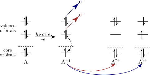
Figure 1: Generation of a core-ionized state (left) and its Auger decay into different channels (right).

The main subject of the present work is the description of Auger decay of core-ionized states, but many of our conclusions hold for resonant Auger decay and more involved processes as well. A particular topic that we will deal with is the determination of partial decay widths, that is, the relative probability of decay into a particular channel. In Auger electron spectroscopy,Agarwal (2013) partial decay widths are determined from the kinetic energies of the emitted Auger electrons. The intensity of the Auger electrons is measured as a function of their energy and, typically, each signal can be assigned to a specific decay channel. While the total number of open decay channels can be anticipated by the application of selection rules based on molecular symmetry, the determination of partial decay widths poses a challenge to experiment and theory alike. Agarwal (2013); Manne and Ågren (1985); Zähringer, Meyer, and Cederbaum (1992a, b); Tarantelli, Sgamellotti, and Cederbaum (1994); Yarzhemsky and Sgamellotti (2002); Kolorenc and Averbukh (2011); Inhester et al. (2012, 2014); Skomorowski and Krylov (2021a, b) In a rigorous scattering approach, they may potentially be evaluated by constructing true continuum functions for each channel at the respective energies. However, we consider it desirable to evaluate partial widths from $L^{2}$ integrable wave functions in analogy to molecular properties of bound states, even though this necessarily constitutes an approximation.

A fundamental aspect of core-vacant states is that they are not bound states but metastable electronic resonances.Moiseyev (2011); Jagau, Bravaya, and Krylov (2017) Since they can undergo Auger decay, these states are coupled to the continuum and their lifetime is finite. This is beyond the reach of quantum-chemical methods geared towards bound states. Many existing computational approaches for core-vacant states neglect their metastable character entirely, meaning the decay width is modeled to be zero. An elegant way to impose this restriction in a controlled manner consists in the core-valence separation (CVS).Cederbaum, Domcke, and Schirmer (1980) There is ample evidence Coriani and Koch (2015); Vidal et al. (2019); Fransson et al. (2021) that CVS-based descriptions are highly accurate for many types of core-vacant states as long as one is only interested in energies and molecular properties determined as energy derivatives. However, methods that consider core-vacant states to be bound are obviously unsuited for modeling Auger decay.

There are several theoretical approaches for electronic resonances.Jagau, Bravaya, and Krylov (2017); Moiseyev (2011) Besides approaches based on R-matrix theory,García et al. (2009); Gorczyca (2000) Fano’s theory Fano (1961); Feshbach (1962) is of particular importance for Auger decay. Here, the resonance wave function is modeled as a bound state superimposed by the electronic continuum. An important aspect of methods based on Fano’s theory is that the electronic continuum cannot be properly represented by the $L^{2}$ integrable functions used in bound-state electronic-structure theory. This can be circumvented by modeling the wave function of the emitted Auger electron in an implicit fashion, for example, using Stieltjes imaging.Langhoff and Corcoran (1974); Carravetta and Ågren (1987) Although the problem of a somewhat arbitrary partition of the Hilbert space into a bound and a continuum part persists, this approach is well capable of modeling Auger decay as the popular “Fano-ADC” approachAverbukh and Cederbaum (2005); Kolorenč and Averbukh (2020) illustrates. Here, algebraic diagrammatic constructionSchirmer (1982) (ADC) is used as electronic-structure backend. As an alternative to Stieltjes imaging, more explicit treatments of the Auger electron are possible where one solves an effective one-electron Schrödinger equation with scattering boundary conditions.Zähringer, Meyer, and Cederbaum (1992a, b) Recently, an approach was suggested, where the decaying resonance state is represented as a product of a continuum orbital and a correlated many-body wave function.Skomorowski and Krylov (2021a) This approach has been shown to reproduce the most important signals in Auger spectra reliably, but the functional form of the wave function of the Auger electron has to be assumed a priori, for example, as plane wave or Coulomb wave.

In this work, we seek to put forward an alternative method for the computation of molecular Auger decay widths based on an $L^{2}$ representation of the resonance wave function. This relies on analytic continuation of the Hamiltonian to the complex plane by means of complex scalingAguilar and Combes (1971); Balslev and Combes (1971); Moiseyev (2011) and its extension to molecules based on complex basis functions.McCurdy and Rescigno (1978); Moiseyev and Corcoran (1979) In these methods, the decaying character of the resonance states is implicitly considered in $L^{2}$ integrable wave functions that are eigenstates of a non-Hermitian Hamiltonian and have complex energies. In this way, complex-variable electronic-structure methods offer a unified treatment of bound states and different types of resonances. Their integration into existing implementations of quantum-chemical methodsJagau, Bravaya, and Krylov (2017); Bravaya et al. (2013); Jagau et al. (2014); Zuev et al. (2014); White, Head-Gordon, and McCurdy (2015); White, McCurdy, and Head-Gordon (2015); White et al. (2017) requires extension of the arithmetic to complex numbers and a different normalization of the wave functionMoiseyev, Certain, and Weinhold (1978) but the working equations of a particular quantum-chemical method stay the same and no a priori assumption about the wave function of the emitted electron needs to be made.

Complex scaling has already been applied to atomic Auger decay,Zhang and Yeager (2012a, b); Peng et al. (2016) but no similar applications to molecules have been reported. At the same time, several applications of complex basis functions to other types of resonances such as temporary anionsWhite, Head-Gordon, and McCurdy (2015); White, McCurdy, and Head-Gordon (2015); White et al. (2017) and molecules in static electric fields have been reported recently.Jagau (2018); Thompson, Ochsenfeld, and Jagau (2019); Hernández Vera and Jagau (2019, 2020) We also mention treatments of Auger decay rates and ICD rates based on complex absorbing potentials.Ghosh, Pal, and Vaval (2013, 2015); Ghosh, Vaval, and Pal (2017) This technique affords a treatment of electronic resonances in terms of $L^{2}$ wave functions as well and can be related to complex scaling.Moiseyev (1998); Riss and Meyer (1993, 1998)

Here, we extend the method of complex basis functions to molecular Auger decay. Through energy decomposition analysis of the complex-scaled wave function, we identify key differences between core-ionized states and other types of resonances that involve only valence electrons. These differences give rise to markedly different basis requirements and an overall more robust performance of complex-scaled methods for core-ionized states as compared to other types of resonances. Our work is based on coupled-clusterČížek (1966, 1969); Shavitt and Bartlett (2009) (CC) and equation-of-motion (EOM)-CCEmrich (1981); Sekino and Bartlett (1984); Stanton and Bartlett (1993); Nooijen and Snijders (1993); Stanton and Gauss (1994); Shavitt and Bartlett (2009) wave functions within the singles and doubles approximation (CCSD and EOM-CCSD). These methods provide a parameter-free single-reference description of the many-electron wave function. Several applications to X-ray spectroscopiesCoriani and Koch (2015); Vidal et al. (2019); Skomorowski and Krylov (2021a, b); Zheng and Cheng (2019); Park, Perera, and Bartlett (2019); Frati et al. (2019); Liu et al. (2019); Nanda et al. (2020); Vidal et al. (2020); Vidal, Krylov, and Coriani (2020); Matthews (2020) have illustrated that they are able to provide an excellent description of core-vacant states. However, we anticipate that the analysis of complex-scaled CCSD and EOM-CCSD wave functions presented here will be relevant to other state-of-the-art electronic-structure methods for core-vacant states as well. These include, for example, time-dependent density functional theory (TD-DFT) Besley and Asmuruf (2010) and $\Delta$DFT approaches,Besley, Gilbert, and Gill (2009) ADC methods of second and third orderWenzel, Wormit, and Dreuw (2014a, b); Wenzel et al. (2015); Averbukh and Cederbaum (2005); Kolorenč and Averbukh (2020), and higher-order CC methods.Zheng and Cheng (2019); Liu et al. (2019); Matthews (2020)

The remainder of this article is structured as follows: In Sec. II, we discuss the theory of complex scaling and complex basis functions, some aspects of complex-scaled CC and EOM-CC theory relevant to our work, and the theoretical background of our energy decomposition analysis. In Sec. III we analyze the complex-scaled wave function of Ne⁺ ($1\text{s}^{-1}$) and discuss the implications for the treatment of molecular Auger decay in terms of complex basis functions. On the basis of these results, we present in Sec. IV a computational protocol for the treatment of molecules together with some applications to core-ionized states of H₂O, N₂, and C₆H₆. Our general conclusions and an outlook on possible extensions of the new method are given in Sec. V.

II Theoretical considerations

II.1 Treatment of the continuum by means of complex scaling

In complex scaling (CS) Aguilar and Combes (1971); Balslev and Combes (1971); Moiseyev (2011), the Hamiltonian is subject to an unbounded similarity transformation

$$\hat{H}_{\text{CS}}=\hat{S}\hat{H}\hat{S}^{-1}\text{ with }\hat{S}=\text{e}^{\text{i}\theta r\,\text{d}/\text{d}r}~{},\quad 0<\theta<\uppi/4~{}.$$ (1)

This is equivalent to rotating the electronic coordinates in $\hat{H}(r)$ so that the Hamiltonian becomes $\hat{H}(r\text{e}^{\text{i}\theta})$. The resonances, which are peaks in the density of continuum states in Hermitian quantum mechanics, now attain discrete complex eigenvalues

$$E_{\text{res}}=E_{\text{R}}-\text{i}\Gamma/2,$$ (2)

which are directly related to the resonance position $E_{\text{R}}$ and the resonance width $\Gamma$, the inverse of the state’s lifetime. At the same time, the continua are rotated by an angle of $2\theta$ into the lower-half complex plane.

If the Hamiltonian is represented exactly, only the energies of the continua and the resonances embedded therein are affected by CS, while bound states have Im($E$) = 0 even though their wave functions change. Also, the complex eigenvalues of the resonances are independent of $\theta$ if it is larger than the critical valueBalslev and Combes (1971)

$$\theta_{\text{c}}=1/2\,\text{arctan}[\Gamma/2\,(E_{\text{R}}-E_{\text{t}})]$$ (3)

with $E_{\text{t}}$ as threshold energy. Above the same critical angle, the resonance wave functions are $L^{2}$ integrable and thus amenable to a treatment with bound-state methods. In the context of Auger decay, Eq. (3) implies that very small scaling angles are sufficient to uncover the resonances and make their wave functions $L^{2}$ integrable. If we consider for a back-of-the-envelope estimate the core-ionized state of neon ($\Gamma\approx 0.25$ eV, $E_{\text{R}}-E_{\text{t}}\approx 800$ eV), a scaling angle of less than 0.01^∘ should be sufficient. This is in contrast to, for example, the temporary anion $\text{N}_{2}^{-}$ ($\Gamma\approx 0.4$ eV, $E_{\text{R}}-E_{\text{t}}\approx 2.3$ eV) Jagau, Bravaya, and Krylov (2017) where the critical angle is ca. 5^∘. Core-ionized wave functions are thus on the verge of $L^{2}$ integrability, which distinguishes them from other types of resonances. In actual calculations with a finite basis, $E_{\text{res}}$ does depend on $\theta$; the optimal value is usually found through minimizing $|\text{d}E/\text{d}\theta|$.Moiseyev, Certain, and Weinhold (1978); Jagau, Bravaya, and Krylov (2017) For this purpose, trajectories $E(\theta)$ need to be calculated, which is the main reason that complex-scaled methods are more computationally expensive than their real-valued counterparts.

CS has the major disadvantage that it cannot be applied to molecules because the complex-scaled electron-nuclear attraction is not dilation analytic within the Born-Oppenheimer approximation.Moiseyev (2011) A possible solution is exterior scaling,Simon (1979) where the area close to the nuclei is not scaled. In the context of Gaussian basis sets, this can be realized by the method of complex basis functions (CBFs),McCurdy and Rescigno (1978); Moiseyev and Corcoran (1979) which relies on the identity

$$\frac{\langle\Psi(r)|\hat{H}(r\text{e}^{\text{i}\theta})|\Psi(r)\rangle}{\langle\Psi(r)|\Psi(r)\rangle}=\frac{\langle\Psi(r\text{e}^{-\text{i}\theta})|\hat{H}(r)|\Psi(r\text{e}^{-\text{i}\theta})\rangle}{\langle\Psi(r\text{e}^{-\text{i}\theta})|\Psi(r\text{e}^{-\text{i}\theta})\rangle}$$ (4)

and the fact that scaling the coordinates of the basis functions according to the right-hand side of Eq. (4) is equivalent to scaling their exponents in the same way. Since it is possible to scale only selected basis functions —in the computational practice hitherto the most diffuse shellsWhite, Head-Gordon, and McCurdy (2015)— dilation analyticity is preserved and CBF methods are applicable to molecules.

A further advantage of CBF methods over CS is that changes in the bound-state and resonance wave functions stemming from Eq. (1) are smaller. As a result, Im($E)$ of bound states, which is zero in the full basis-set limit, is smaller by orders of magnitude in CBF calculations than in CS calculations.

We add here that the scaling angle can be chosen to be complex-valued in CBF and CS methods, that is, $\text{e}^{-\text{i}\theta}=\alpha\cdot\text{e}^{-\text{i}\theta_{\text{R}}}$; $\alpha,\theta_{\text{R}}\in\mathbb{R}$. Moiseyev and Corcoran (1979); Moiseyev (2011) The factor $\alpha$ represents an optimization of the exponents of the basis functions and is related to the stabilization method where resonances are identified from changes in the energy upon scaling the exponents.Hazi and Taylor (1970); Taylor and Hazi (1976)

CBF methods offer access to different types of molecular electronic resonances as illustrated by many recent applications.White, Head-Gordon, and McCurdy (2015); White, McCurdy, and Head-Gordon (2015); White et al. (2017); Jagau (2018); Hernández Vera and Jagau (2019, 2020) However, no work on molecular Auger decay has been reported. As we will show in Sec. III, a straightforward application of computational protocols developed for other resonances results in zero decay widths, that is, such CBF calculations are blind to Auger decay. Several changes are necessary to uncover the decaying character of core-ionized states.

II.2 Complex-variable coupled-cluster methods

In CC theory, the wave function is obtained from the Hartree-Fock (HF) state $|\Psi_{0}\rangle$ by the action of the cluster operator $\hat{T}$ according to

$$|\Psi_{\text{CC}}\rangle=\text{e}^{\hat{T}}|\Psi_{0}\rangle=(1+\hat{T}+\hat{T}^{2}/2!+\hat{T}^{3}/3!+\dots)|\Psi_{0}\rangle~{}.$$ (5)

In CBF-CC methods, $|\Psi_{0}\rangle$ is always complex-valued while different approaches are possible for CS-CC methods.Bravaya et al. (2013); Jagau, Bravaya, and Krylov (2017) In this work, all CS calculations are based on a CS-HF reference.

Inclusion of different excitation levels in $\hat{T}$ gives rise to a hierarchy of methods that converges smoothly to the exact solution. Here, we use CCSD where $\hat{T}=\hat{T}_{1}+\hat{T}_{2}$. The exponential parametrization in Eq. (5) ensures size-extensivity and inclusion of the most relevant higher excitations through products of $T_{1}$ and $T_{2}$. Shavitt and Bartlett (2009)

Inserting Eq. (5) into the Schrödinger equation, one obtains

$$\hat{H}\text{e}^{\hat{T}}|\Psi_{0}\rangle=E\text{e}^{\hat{T}}|\Psi_{0}\rangle\quad\Leftrightarrow\quad\text{e}^{-\hat{T}}\hat{H}\text{e}^{\hat{T}}|\Psi_{0}\rangle=E|\Psi_{0}\rangle,$$ (6)

where $\text{e}^{-\hat{T}}\hat{H}\text{e}^{\hat{T}}=\bar{H}$ is the similarity-transformed Hamiltonian. Projection of Eq. (6) onto the HF determinant and the singly and doubly excited determinants determines the CCSD energy and amplitudes, respectively.

To describe core-ionized states subject to Auger decay within CC theory, we employ two computational strategies as illustrated in Fig. 2: In the $\Delta$CCSD approach, one performs two separate CCSD calculations based on HF determinants for the neutral state and the core-ionized state. In this work, the latter state is always described in a spin-unrestricted manner. We determine the optimal scaling angle from the difference of the two CCSD energies; in accordance with previous reportsWhite et al. (2017) we find that this approach usually leads to much smaller values for $|\text{d}E/\text{d}\theta|$ than determining $\theta$ from the total energy. If not specified otherwise, we recomputed all energies in the 0–45^∘ range in steps of 1^∘. The total decay width $\Gamma$ is then evaluated from the difference of the two imaginary energies. We reiterate that Im($E$) of the neutral state would be zero in exact theory, but has a significant value especially in CS-based calculations (see Sec. II.1).

The other method we use is EOMIP-CCSD.Nooijen and Snijders (1993); Stanton and Gauss (1994) Based on a CCSD wave function for a neutral molecule, biorthogonal right and left wave functions for a core-ionized state are constructed in EOMIP-CCSD as

$$|\Psi_{\text{EOMCC}}\rangle =\hat{R}\text{e}^{\hat{T}}|\Psi_{0}\rangle~{},$$ (7)

$$\langle\Psi_{\text{EOMCC}}| =\langle\Psi_{0}|\hat{L}^{\dagger}\text{e}^{-\hat{T}}~{}.$$ (8)

Here, the excitation operators $\hat{R}$ and $\hat{L}$ are truncated at the same level as $\hat{T}$, meaning that they include 1-hole ($1\text{h}$) and 2-hole-1-particle ($2\text{h}1\text{p}$) excitations in EOMIP-CCSD. Insertion of Eq. (7) into the Schrödinger equation and projection onto the $1\text{h}$ and $2\text{h}1\text{p}$ excitation manifolds results in an eigenvalue equation for $\bar{H}$. The total decay width $\Gamma$ is directly obtained from the imaginary part of the eigenvalues according to Eq. (2). The optimal scaling angle is also determined from these eigenvalues of the EOMIP-CCSD equations.

The computational cost of both approaches scales as $N^{6}$ with system size. However, while $\Delta$CCSD involves two separate CCSD calculations with $N_{\text{occ}}^{2}N_{\text{virt}}^{4}$ cost, one needs to carry out only one such calculation for the reference state in the EOMIP-CCSD approach; the EOMIP step itself scales as $N_{\text{occ}}^{2}N_{\text{virt}}^{3}$. As a consequence, the EOMIP-CCSD approach typically entails lower computational cost.

All calculations presented in this article were carried out with the complex-variable CCSD and EOM-CCSD codes Bravaya et al. (2013); Zuev et al. (2014) implemented in the Q-Chem software.Epifanovsky et al. (2021)

II.3 Structure of the core-ionized wave function

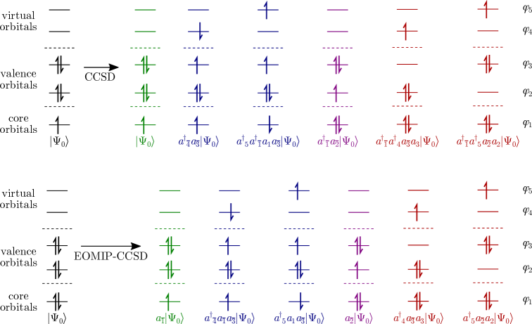
Figure 2: Determinants included in CCSD (upper part) and EOMIP-CCSD (lower part) wave functions for a core-ionized state in a Hilbert space spanned by 5 orbitals. See text for further explanation.

Fig. 2 displays the structures of the complex-scaled CCSD and EOMIP-CCSD wave functions of a core-ionized state, which shows that both methods are capable of describing Auger decay: this is primarily achieved by means of the doubly-excited determinants marked in red, where the core hole has been filled with an electron, while a second valence electron has been excited into the virtual space.

Our numerical results (see Sec. III) confirm that the red configurations in Fig. 2 are almost exclusively responsible for the decay width in the $\Delta$CCSD approach as one would expect. This is, however, not the case in EOMIP-CCSD as we will discuss also in Sec. III. In both approaches, the red determinants are of very minor relevance for the real part of the energy and their amplitudes are typically orders of magnitude smaller than those of the blue configurations. This corroborates the validity of CVS methods since the CVS projector precisely removes the red determinants from the wave function.Cederbaum, Domcke, and Schirmer (1980)

The green determinants represent zeroth-order descriptions of the core-vacant state and, while they carry by far the largest weight in the wave functions, are not relevant to our further analysis. The blue determinants comprise single and double excitations and represent orbital relaxation as well electron correlation effects. They play different roles in $\Delta$CCSD and EOMIP-CCSD: In the latter approach, the HF wave function $|\Psi_{0}\rangle$ is optimized for the neutral ground state and electron correlation is subsequently treated for this state as well. The blue determinants are thus indispensable in EOMIP-CCSD to model the substantial relaxation in the charge distribution due to the core hole as well as differential electron correlation. In the former approach, i. e. $\Delta$CCSD, relaxation effects are already contained in $|\Psi_{0}\rangle$ through changed orbital shapes and energies. The doubly-excited blue determinants thus describe primarily electron correlation and their singly-excited counterparts secondary relaxation effects resulting therefrom.

II.4 Energy decomposition analysis and partial decay widths

To substantiate the qualitative discussion from the preceding section, we use energy decomposition analysis. This allows us to identify contributions from individual excitations to the imaginary energy, that is, the total decay width. In addition, we get access to partial widths corresponding to decay into particular channels.

For $\Delta$CCSD, we use two approaches. We either decompose directly the CCSD energy

$$E=E_{\text{HF}}+\sum_{ijab}\Big{(}\frac{1}{4}t_{ij}^{ab}+\frac{1}{2}t_{i}^{a}t_{j}^{b}\Big{)}\;\langle ij||ab\rangle$$ (9)

or, alternatively, use an expression in terms of the reduced one-electron and two-electron CCSD density matrices $\mathbf{D}^{\text{CCSD}}$ and $\bm{\Gamma}^{\text{CCSD}}$. The latter reads

$$E =\langle\Psi_{0}\,|\,(1+\hat{\Lambda})\,\text{e}^{-\hat{T}}\hat{H}\text{e}^{\hat{T}}\,|\,\Psi_{0}\rangle$$

$$=E_{\text{HF}}+\sum_{pq}\,f_{pq}\,\langle\Psi_{0}|(1+\hat{\Lambda})\text{e}^{-\hat{T}}\{p^{\dagger}q\}\text{e}^{\hat{T}}|\Psi_{0}\rangle$$

$$\quad+\frac{1}{4}\sum_{pqrs}\langle pq||rs\rangle\,\langle\Psi_{0}|(1+\hat{\Lambda})\text{e}^{-\hat{T}}\{p^{\dagger}q^{\dagger}sr\}\text{e}^{\hat{T}}|\Psi_{0}\rangle$$

$$=\,E_{\text{HF}}\,+\,\sum_{pq}D^{\text{CCSD}}_{pq}\,f_{pq}\,+\,\frac{1}{4}\,\sum_{pqrs}\,\Gamma^{\text{CCSD}}_{pqrs}\,\langle pq||rs\rangle$$ (10)

with $\hat{\Lambda}$ as the well-known deexcitation operator from CC gradient theory Shavitt and Bartlett (2009) and $f_{pq}$ and $\langle pq||rs\rangle$ as elements of the Fock matrix and antisymmetrized two-electron integrals, respectively.

For EOMIP-CCSD, the corresponding expression reads

$$E =\langle\Psi_{0}\,|\,\hat{L}^{\dagger}\,\text{e}^{-\hat{T}}\hat{H}\text{e}^{\hat{T}}\,\hat{R}\,|\,\Psi_{0}\rangle$$

$$=E_{\text{HF}}+\sum_{pq}\,f_{pq}\,\langle\Psi_{0}|\hat{L}^{\dagger}\,\text{e}^{-\hat{T}}\{p^{\dagger}q\}\text{e}^{\hat{T}}\,\hat{R}|\Psi_{0}\rangle$$

$$\quad+\frac{1}{4}\sum_{pqrs}\langle pq||rs\rangle\,\langle\Psi_{0}|\hat{L}^{\dagger}\,\text{e}^{-\hat{T}}\{p^{\dagger}q^{\dagger}sr\}\text{e}^{\hat{T}}\,\hat{R}|\Psi_{0}\rangle$$

$$=\,E_{\text{HF}}\,+\,\sum_{pq}D^{\text{EOMIP}}_{pq}\,f_{pq}\,+\,\frac{1}{4}\,\sum_{pqrs}\,\Gamma^{\text{EOMIP}}_{pqrs}\,\langle pq||rs\rangle$$ (11)

and differs from Eq. (II.4) thus only in the definition of the density matrices $\mathbf{D}^{\text{EOMIP}}$ and $\bm{\Gamma}^{\text{EOMIP}}$.

To compute partial widths from Eq. (9), we use a modified $\hat{T}_{2}$ operator, where amplitudes corresponding to a particular decay channel have been set to zero. For the corresponding decomposition based on Eqs. (II.4) and (II.4), we use modified density matrices: After convergence of the CCSD or EOMIP-CCSD equations, we set to zero the amplitudes in $\hat{T}$ and $\hat{\Lambda}$ or $\hat{R}$ and $\hat{L}$ that correspond to a particular decay channel. For EOMIP-CCSD, this is done such that spin-completeness is preserved. We note that decay into a particular channel is usually represented by multiple excitations that differ in the energy of the virtual orbital (see Fig. 2). Using these approaches, we can disable Auger decay channel by channel until we arrive at versions of $\hat{T}$, $\hat{\Lambda}$, $\hat{R}$, and $\hat{L}$ that are used in CVS-CCSD and CVS-EOMIP-CCSD. When evaluated from these CVS-like operators, Eqs. (9)–(II.4) yield zero decay widths.

III Numerical Analysis of Auger Decay of $\text{Ne}^{+}$ ($1\text{s}^{-1}$)

As alluded to in Sec. II.1, the application of computational protocols developed for other types of resonances works well for CS but not for CBF methods. To analyze this further, we use the 1s^-1 state of the neon atom as a test case. This system is a simple and frequently studied example of Auger decay.Skomorowski and Krylov (2021b); Howat et al. (1977); Albiez et al. (1990); Coreno et al. (1999); Müller et al. (2017) There are five main decay channels leading to the ¹D ($2\text{p}^{-2}$), ¹S ($2\text{p}^{-2}$), ³P ($2\text{s}^{-1}2\text{p}^{-1}$), ¹P ($2\text{s}^{-1}2\text{p}^{-1}$), and ¹S ($2\text{s}^{-2}$) states of Ne²⁺.

III.1 Total Auger decay width from complex scaling

Table 1: Energies and half-widths of Ne⁺ (1$\text{s}^{-1}$) computed with CS-EOMIP-CCSD and CS-$\Delta$CCSD using different basis sets. The basis-set suffix +3s3p refers to the addition of 3 diffuse s and p shells with an even-tempered exponent spacing of 2. Energies in eV. Half-widths in meV. Results for additional basis sets can be found in the SI.

Method	Basis set	$\theta_{\text{opt}}/^{\circ}$	$\text{Re}(E)$	$\text{Im}(E)$
EOMIP-CCSD	aug-cc-pCVTZ+6s6p6d	No minimum in $|\text{d}E/\text{d}\theta|$
EOMIP-CCSD	cc-pCVQZ	No minimum in $|\text{d}E/\text{d}\theta|$
EOMIP-CCSD	aug-cc-pCVQZ	10	871.26	$-73$
EOMIP-CCSD	cc-pCV5Z	11	871.22	$-113$
EOMIP-CCSD	aug-cc-pCV5Z	13	871.20	$-114$
EOMIP-CCSD	aug-cc-pCV5Z+3s3p	14	871.20	$-109$
EOMIP-CCSD	cc-pCV6Z	12	871.22	$-97$
$\Delta$CCSD	aug-cc-pCV5Z	12	869.53	$-104$
$\Delta$CCSD	aug-cc-pCV5Z+3s3p	13	869.53	$-101$
Fano			870.12${}^{\text{a}}$	$-109^{\text{b}}$
Experiment	—	—	870.17${}^{\text{a}}$	$-129^{\text{c}}$

Tab. 1 shows core-ionization energies and Auger decay widths of Ne⁺ computed with CS-EOMIP-CCSD and CS-$\Delta$CCSD. This confirms the conclusion from Sec. II.3 that both methods are able to describe Auger decay. $\Delta$CCSD yields a somewhat more accurate result for the ionization energy as compared to EOMIP-CCSD, which is in line with previous findings using real-valued CC methods.Zheng and Cheng (2019); Matthews (2020) The decay widths differ by less than 10 % and are well in line with earlier theoretical results.Skomorowski and Krylov (2021b) The underestimation of the decay width by 10-20 % as compared to the experimental valueMüller et al. (2015) can be related to the fact that double Auger decay and other processes involving more than two electrons are not described within the CCSD approximation. The corresponding decay channels are not present in our calculations.

Tab. 1 also illustrates that extra diffuse shells are not needed to describe Auger decay of Ne⁺. This is unlike to low-lying temporary anions and Stark resonances formed in static electric fields, where these extra shells are vital to obtain accurate decay widths with CS methods.White, Head-Gordon, and McCurdy (2015); White et al. (2017); Hernández Vera and Jagau (2020) On the other hand, requirements towards the valence part of the basis set are as high as in CS calculations of other types of resonances. It appears that aug-cc-pCVQZ is the smallest basis set that is able to capture the decaying character of the wave function and even this basis set recovers only 2/3 of the decay width computed with aug-cc-pCV5Z.

III.2 Partial Auger decay widths from complex scaling

To compute partial decay widths, we decomposed the total CS-CCSD decay width of Ne⁺ ($1\text{s}^{-1}$) on the basis of Eqs. (9) and (II.4) by setting to zero amplitudes in $\hat{T}_{2}$ and $\hat{\Lambda}_{2}$ that create the “red” determinants in Fig. 2. Our results are compiled in Tab. 2 and compared with results obtained using a combination of Fano’s approach with EOM-CC theorySkomorowski and Krylov (2021b) as well as with experimental values.Müller et al. (2017); Albiez et al. (1990) As branching ratios and total decay widths are usually determined by separate experiments, we derived the experimental values for the partial widths in Tab. 2 by multiplying branching ratios from Ref. 90 with the result of a recent measurement of the total decay width.Müller et al. (2017)

Table 2: Partial decay half-widths for the 5 decay channels of Ne⁺ ($1\text{s}^{-1}$). All values in meV.

Decay channel	CS/$\Delta^{\text{a}}$	CS/$\Delta^{\text{b}}$	CS/EOM${}^{\text{c}}$	Fano${}^{\text{d}}$	Experiment${}^{\text{e}}$
all	122.3	133.7	210.9	109.1	128.5(30)
1D (2p-2)	74.7	81.5	133.4	58.8	78.2(21)
1P (2s-12p-1)	27.7	29.3	21.6	19.6	22.1(7)
3P (2s-12p-1)	6.6	6.6	43.2	11.9	8.1(3)
1S (2s-2)	9.3	8.8	1.0	13.6	7.9(3)
1S (2p-2)	7.0	7.6	12.8	5.3	12.2(4)

Tab. 2 illustrates overall excellent agreement between our CS-CCSD partial widths and those from experiment; the experimental values are reproduced with a root mean square deviation of 4 meV. However, there are several issues that deserve a discussion:

First, the half-widths computed with Eqs. (9) and (II.4) are not identical. This is due to the structure of the CCSD density matrices in Eq. (II.4): A term such as $\hat{\Lambda}_{\text{d-decay}}\cdot\hat{T}_{\text{s-decay}}$ is set to zero when computing the partial widths for either decay channel and thus counted twice. This also causes that the sum of the partial half-widths of the 5 channels (125 meV) is not identical to the total half-width in Tab. 2 (122 meV). On the other hand, no double counting occurs in Eq. (9) and the corresponding partial widths are strictly additive.

A second observation is that neither Eq. (9) nor Eq. (II.4) yield half-widths that sum up to the total CS-CCSD half-width reported in Tab. 1. When removing all determinants marked in red in Fig. 2, we obtain values of 134 and 122 meV from Eqs. (9) and (II.4), respectively, whereas the value from Tab. 1 is 104 meV.

This discrepancy stems from three origins: First, $\Gamma/2$ in Tab. 1 is evaluated from the energy difference between the core-ionized and the neutral ground state, whereas Eqs. (9) and (II.4) are applied only to the core-ionized state. Second, the “red” determinants in Fig. 2 contribute to $\Gamma/2$ not only through $\hat{T}_{2}$ but also through $\hat{T}_{1}\cdot\hat{T}_{1}$. Third, the determinants marked in blue and purple in Fig. 2 deliver a non-negligible contribution to $\Gamma/2$, but their assignment to a particular decay channel is not straightforward. We neglected these contributions in the values reported in Tab. 2 but we note that the “blue” determinants are related to shake-up and shake-off processes, which are well known in the context of interchannel coupling in Auger decay.Howat et al. (1977); Colle and Simonucci (1990)

An equivalent decomposition of the EOMIP-CCSD decay width was performed on the basis of Eq. (II.4) by setting to zero elements of $\hat{R}_{2}$ and $\hat{L}_{2}$. These results are also contained in Tab. 2. It is apparent that the EOMIP-CCSD partial widths are very unreliable: By removing all excitations into the “red” determinants from $\hat{R}_{2}$ and $\hat{L}_{2}$, we obtain for $\Gamma/2$ a value of 211 meV from Eq. (II.4), whereas the imaginary part of the eigenvalue of the EOMIP-CCSD equations is 114 meV (see Tab. 1).

The reasons for this failure are similar in origin to the much smaller discrepancies between the CCSD values discussed before. First, Eq. (II.4) is an expression for $E-E_{\text{HF}}$, while the EOMIP-CCSD equations yield $E-E_{\text{CCSD}}$ as eigenvalue. Albeit zero in exact theory, the imaginary energy of the neutral CCSD reference state amounts to $\sim 1.3\cdot 10^{-3}$ a.u. or 35 meV in our calculations. Second, the “blue” and “purple” determinants from Fig. 2 are again neglected. Third, the “red” determinants in Fig. 2 cannot only be created by $\hat{R}_{2}$ but also by combinations of $\hat{R}_{1}$ and $\hat{T}_{2}$ as well as $\hat{R}_{1}$ and $\hat{T}_{1}$. These contributions to $\Gamma/2$ are substantial and their neglect is the reason that we observe much larger discrepancies between Tabs. 1 and 2 for EOMIP-CCSD than for $\Delta$CCSD.

III.3 Analysis of the orbital basis

To understand the basis-set dependence documented in Tab. 1, we decomposed the CS-CCSD partial decay width of the ¹D(2p^-2) channel further into contributions from different excitations. The 8 d shells in the aug-cc-pCV5Z basis for Ne give rise to 8 sets of virtual orbitals with d-symmetry. We computed their contributions to $\Gamma/2$ by setting to zero in Eq. (II.4) those amplitudes $t_{ij}^{ab}$ and $\lambda_{ab}^{ij}$ where $i=j=2\text{p}$ and $a=1\text{s}$, $b=n\text{d}$ or $a=n\text{d}$, $b=1\text{s}$. The results are presented in Tab. 3 together with the corresponding orbital energies.

Table 3: Contributions $\Delta$Im($E$) of different d orbitals ($n=3-10$) in meV to the CS-CCSD partial half width of the ¹D(2p^-2) channel of Ne⁺($1\text{s}^{-1}$) computed with the aug-pCV5Z basis set at $\theta_{\text{opt}}=12^{\circ}$. All orbital energies $\varepsilon$ in a.u. and the three-particle overlaps $O$ (in ų Bohr^-4.5) of the d orbitals with the 2p orbitals are also given. See text for further details.

$n$	$\Delta$Im($E$)	Re($O$)	Im($O$)	Re($\varepsilon$)	Im($\varepsilon$)
3	$-$0.1	$-0.9$	2.8 $\cdot 10^{-8}$	0.60	$-$0.27
4	$-$1.6	3.5	$-$7.3 $\cdot 10^{-8}$	1.88	$-$0.79
5	$-$6.5	7.4	1.4 $\cdot 10^{-7}$	4.79	$-$2.12
6	$-$18.0	8.8	5.8 $\cdot 10^{-7}$	12.11	$-$5.74
7	$-$46.7	5.8	7.2 $\cdot 10^{-7}$	31.61	$-$15.81
8	$-$2.6	$-$1.9	$-$4.5 $\cdot 10^{-7}$	88.28	$-$45.27
9	$-$0.1	0.4	9.6 $\cdot 10^{-8}$	259.60	$-$132.53
10	$-$0.0	0.1	1.5 $\cdot 10^{-8}$	791.25	$-$399.75

Tab. 3 illustrates that the ¹D partial decay width arises almost exclusively from excitations into determinants in which the 5d, 6d, and 7d orbitals are occupied, while excitations into the remaining d orbitals contribute only 6 %. We note that for the 7d orbital, which delivers the largest contribution to $\Gamma/2$, Re($\varepsilon$) $\approx$ 860 eV, which is close to the kinetic energy of the emitted Auger electron (804 eV).Albiez et al. (1990) This observation offers an explanation why scaling of diffuse basis functions is necessary for the description of low-lying temporary anions, where the outgoing electron has just a few eV, while functions with larger exponent need to be scaled to describe Auger decay. This is the reason why calculations in which only diffuse functions are scaled are blind to Auger decay.

To analyze this further, we computed the values of the d${}_{xy}^{\upalpha}$ orbitals along the $xy$ diagonal at $z=0$ and compared them to those of the 2p${}_{x}^{\upalpha}$ and 2p${}_{x}^{\upbeta}$ orbitals. Along this line, the aforementioned orbitals have no nodal plane due to the angular part that would complicate the analysis. Plots of the real and imaginary parts of the 2p${}_{x}^{\upbeta}$ orbitals and a few selected d${}_{xy}^{\upalpha}$ orbitals are presented in Fig. 3. As shown in the SI, the differences between the 2p${}_{x}^{\upalpha}$ and 2p${}_{x}^{\upbeta}$ orbitals are small and not relevant for the further discussion.

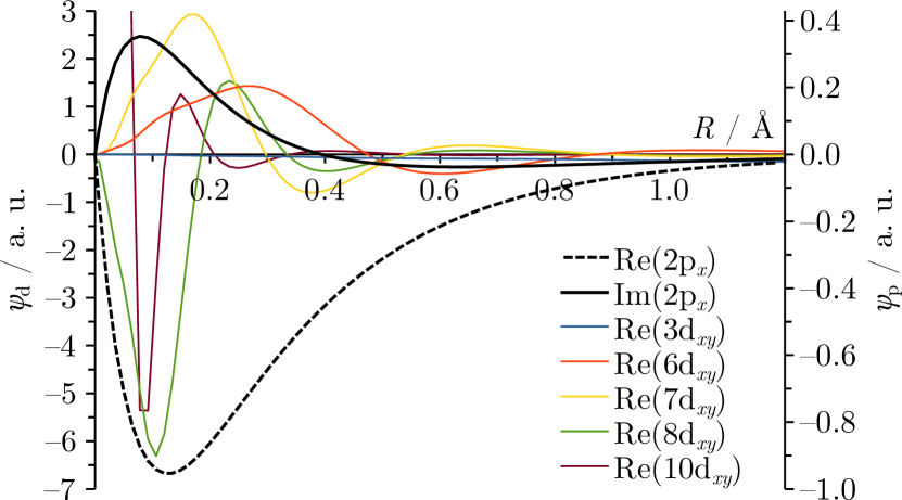
Figure 3: Plots of the 2p${}_{x}^{\upbeta}$ and selected d${}_{xy}^{\upalpha}$ orbitals along the $xy$ diagonal obtained from a CS-UHF calculation for Ne⁺($1\text{s}_{\upalpha}^{-1}$) using the aug-cc-pCV5Z basis set.

The d orbital with the lowest energies (e. g. 3d_xy) are very diffuse and reach their maximum amplitude at a distance of 1.3 Å from the nucleus, where the amplitude of the 2p_x orbital is negligible. On the other hand, the d orbitals with high energies (e. g. 10d_xy) have strong oscillations close to the nucleus. Only the d orbitals in between (e. g. 6d_xy, 7d_xy), which together yield more than 90 % of the decay width, have large amplitudes close to the nucleus and at the same time no node less than 0.3 Å away from it so that their overlap with the 2p_x orbital is large.

We quantify this overlap by integrating over the radial coordinate of the product of three orbitals as follows:

$$O=\int_{0}^{\infty}\text{d}r\;4\uppi r^{2}\;\varphi_{\text{2p},x}^{\upalpha}(r)\;\varphi_{\text{2p},y}^{\upbeta}(r)\;\varphi_{n\text{d},xy}^{\upalpha}(r)~{}.$$ (12)

Eq. (12) is formulated for decay into the ¹D state of Ne²⁺ but can be easily generalized to other systems. We note that, because p orbitals are ungerade and d orbitals are gerade, only the three-orbital overlap defined according to Eq. (12) is nonzero, whereas the integral over a simple product of 2p_x and $n$d_xy along the $xy$ diagonal would vanish.

The values for $O$ calculated from Eq. (12) are listed in Tab. 3. This shows that Re($O$) and Im($O$) are indicators of the contribution of a particular d orbital to the decay width; the d orbitals with the largest overlaps with 2p_x also contribute most to $\Gamma/2$. The description of Auger decay in the CS-CCSD wave function thus relies on the overlap between the valence orbitals which are emptied during the decay process and the virtual orbitals, in which the outgoing electron is quenched. The quantity $O$ from Eq. (12) is presumably useful as well for analyzing the description of other states that decay by a two-electron process, i. e., Feshbach resonances in general.

Our calculations show that the largest contribution to Im($O$) stems from $[\text{Im}(\varphi_{2\text{p},x})\cdot\text{Re}(\varphi_{2\text{p},y})+\text{Re}(\varphi_{2\text{p},x})\cdot\text{Im}(\varphi_{2\text{p},y})]\cdot\text{Re}(\varphi_{n\text{d},xy})$. For the values in Tab. 3, this term is more than 10 times larger than those involving $\text{Im}(\varphi_{n\text{d},xy})$, in line with the nodal structures of the orbitals shown in Fig. 3.

As a further step, we analyzed the molecular orbital coefficients of the d orbitals that deliver the largest contributions to the ¹D decay width (5d, 6d, 7d). The results are compiled in Tab. 4; it is evident that basis functions with intermediate exponents between 1 and 10 are responsible for the largest share of the decay width.

This explains again the basis-set dependence documented in Tab. 1: Diffuse basis functions produce low-lying virtual orbitals that do not overlap with the occupied valence orbitals, while steep basis functions lead to virtual orbitals with high energy, whose overlap with the occupied orbitals cancels out due to oscillations. Only the intermediate virtual orbitals with an energy in the range of that of the emitted Auger electron overlap substantially with the valence orbitals and thus contribute to the Auger decay width.

Table 4: Real parts of molecular orbital coefficients of selected d^α orbitals obtained from a CS-UHF calculation for Ne⁺ (1$\text{s}_{\upalpha}^{-1}$) using the aug-cc-pCV5Z basis set.${}^{\text{a}}$

Exponent	Contribution to MO
of bf	5d	6d	7d
212	$-0.0009$	$0.003$	$-0.01$
75.8	$0.005$	$-0.01$	$0.06$
27.0	$-0.02$	$0.07$	$-0.2$
9.84	$0.1$	$-0.2$	1.7
3.84	$-0.2$	1.7	–1.7
1.50	1.6	–1.7	$1.0$
0.587	–1.4	$0.8$	$-0.4$
0.213	$0.5$	$-0.3$	$0.1$

III.4 Total and partial Auger decay widths from complex basis functions

Having identified the most important basis functions for the description of Auger decay in in CS-CC calculations, we are now in a position to conduct CBF-CCSD and CBF-EOMIP-CCSD calculations; the results are shown in Tab. 5. We started by scaling all functions in the aug-cc-pCV5Z basis set and then proceeded by scaling fewer and fewer functions as illustrated in Tab. 5. For technical reasons, the unscaled STO-2G basis had to be added to some calculations. Some additional results computed with other choices of scaled basis functions are available from the SI.

Table 5: Energies and half-widths of Ne⁺ (1$\text{s}^{-1}$) computed with CBF-EOMIP-CCSD and CBF-$\Delta$CCSD by scaling different parts of the basis set. Energies in eV. Half-widths in meV.

Method	Scaled bfs${}^{\text{a}}$	$\theta_{\text{opt}}/^{\circ}$	$\text{Re}(E)$	$\text{Im}(E)$
Basis set: STO-2G + aug-cc-pCV5Z
$\Delta$CCSD	aug-cc-pCV5Z	10	869.53	$-109$
EOMIP-CCSD	aug-cc-pCV5Z	11	871.20	$-116$
EOMIP-CCSD	4D, 2D, 0.6D, 0.2D,	13	871.18	$-118$
	1P, 2S, 3F, 1F
Basis set: aug-cc-pCV5Z
$\Delta$CCSD	4D	17	869.49	$-100$
EOMIP-CCSD	10D, 4D, 2D	18	871.21	$-71$
EOMIP-CCSD	4D	21	871.18	$-89$
EOMIP-CCSD	4S	24	871.04	$-20$
EOMIP-CCSD	4D, 2D, 0.6D, 0.2D,	6	871.08	$-124$
	1P, 2S, 3F, 1F
Reference values
CS-$\Delta$CCSD / aug-cc-pCV5Z		12	869.53	$-104$
CS-EOMIP-CCSD / aug-cc-pCV5Z		13	871.20	$-114$
Fano			870.12 Coreno et al. (1999)	$-109$ Skomorowski and Krylov (2021b)
Experiment			870.17 Coreno et al. (1999)	$-129$ Müller et al. (2017)

The results in Tab. 5 demonstrate that CBF-$\Delta$CCSD and CBF-EOMIP-CCSD both reproduce the CS reference values from Tab. 1 to an excellent degree when all basis functions are scaled. When we instead scale only the three d shells with the largest contribution to $\Gamma/2$ (see Tab. 4), we still reproduce 95 % of the ¹D partial decay width from Tab. 2. However, our results indicate that the scaled part of the basis set can be reduced further: With a single scaled d shell (exponent = 3.844), we obtain 120 % of the CS-CCSD value for the ¹D partial width. The same procedure is also successful for the two ¹S decay channels: Scaling one s function (exponent = 4.327) results in 120 % of the CS-CCSD partial widths for these channels. Furthermore, by scaling a total of 8 s, p, d, and f shells, we recover the total decay width up to a few percent.

It thus appears that one can compute partial decay widths with CBF methods by scaling only basis functions of the respective angular momentum. However, for decay into the ¹P and ³P channels, we encountered convergence problems or obtained qualitatively incorrect results in calculations with a single scaled p shell. This problem presumably arises because decay into the ¹P and ³P channels involves the occupied 2p orbital and additionally some virtual p orbitals. Complex scaling a p shell thus affects the description of the occupied 2p orbital, whereas for the ¹D (2p^-2) and ¹S (2p^-2) channels the involved occupied orbitals (2p) are of a different angular momentum than the relevant virtual orbitals (d or s, respectively). As documented in the SI, a solution to this problem is to add complex-scaled functions to a basis set instead of scaling functions that are already contained in the basis set. In this way, the consistency of the predefined basis is preserved.

A further detail in Tab. 5 worth mentioning are the differences in $\theta_{\text{opt}}$ between the decay channels. Using Eqs. (9) and (II.4), the CS-CCSD partial widths are evaluated at the same $\theta$ and thus not at the respective $\theta_{\text{opt}}$ but this does not seem to affect the quality of the partial widths obtained with this approach as Tab. 2 illustrates.

III.5 Truncation of the complex-scaled basis set

At this point, two questions still need to be answered to compute Auger decay rates in a black-box fashion with CBF methods: First, how to choose the complex-scaled functions that are added to a predefined basis set and, second, how to truncate the aug-cc-pCV5Z basis set that we used so far without compromising accuracy.

To investigate the requirements on the complex-scaled exponents, we performed series of CBF-EOMIP-CCSD calculations where we added one additional s, p, or d shell with varying exponent to the aug-cc-pCV5Z basis set. For each value of the exponent, a trajectory $E(\theta)$ was computed. This procedure is equivalent to optimizing the exponent of the extra shell in the complex number plane.Moiseyev (2011) The resulting decay half-widths are presented in Fig. 4 together with the value of $|\text{d}E$/d$\theta|$ at the respective $\theta_{\text{opt}}$.

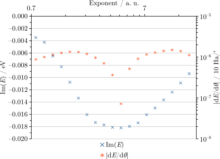
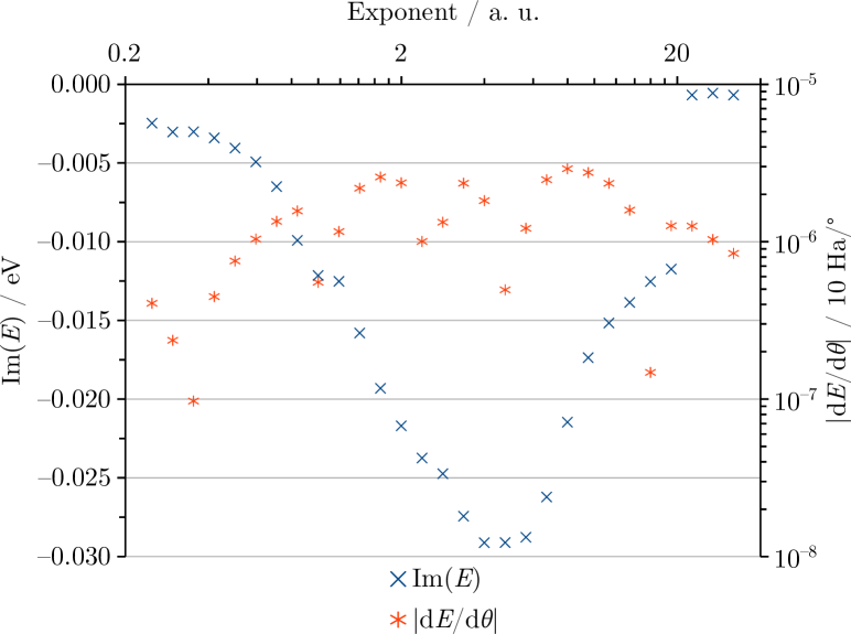
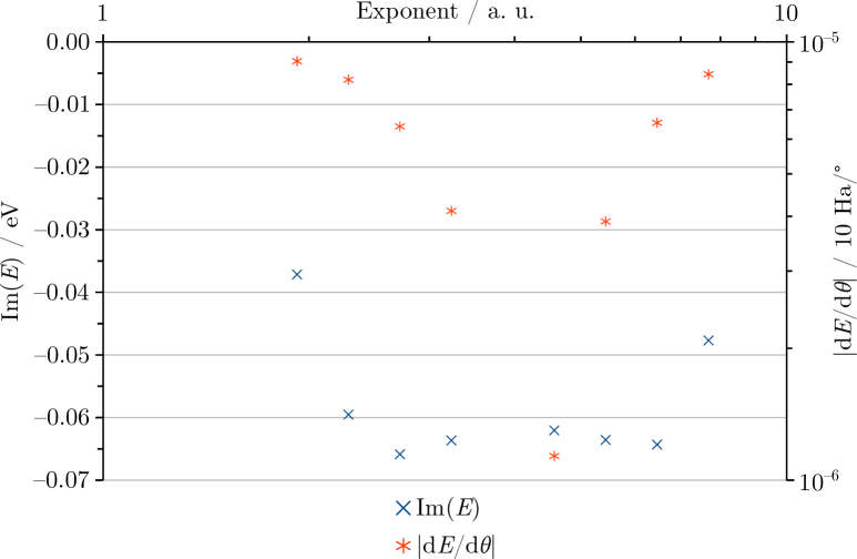
Figure 4: Decay half-widths $-\text{Im}(E)$ and stabilizations $|\text{d}E/\text{d}\theta|$ of Ne⁺ (1s^-1) computed with CBF-EOMIP-CCSD/aug-cc-pCV5Z as a function of the exponent of the single complex-scaled shell that was added to the basis set. $\theta$ was optimized for each exponent. The complex-scaled shell is an s, p, d shell in the upper, middle, and lower panel, respectively.

All three panels of Fig. 4 have in common that the decay width is only captured when the exponent of the complex-scaled shell falls in a specific range spanning ca. one order of magnitude. Outside these ranges, Im($E$) quickly approaches zero. The extrema in Im($E$) observed in Fig. 4 at 18 meV (scaled s function, exponent 4.33), at 29 meV (scaled p shell, exponent 4.00), and at 66 meV (scaled d shell, exponent 2.72) are very well in line with the partial widths obtained through decomposition of the CS-CCSD energy and also accurate estimates of the experimental values (see Tab. 2). In the SI, we demonstrate through decomposition of the CBF-CCSD energy according to Eq. (II.4) that decay widths obtained as in Fig. 4 indeed stem from only those channels that correspond to the angular momentum of the complex-scaled shell.

Table 6: Partial decay half widths of Ne⁺ (1$\text{s}^{-1}$) computed with CBF-EOMIP-CCSD and various basis sets. All values in meV.

	# of	Complex	$-\,\text{Im}(E)$
Basis set	b.f.s	shells${}^{\text{a}}$	D	P	S	allb
aug-cc-pCV5Z	181	opt.	64	31	19	114
aug-cc-pCVQZ	109	opt.	67	51	15	132
aug-cc-pCVQZ	109	from 5Z	67	19	20	106
aug-cc-pCVTZ	59	opt.	90	4	36	130
aug-cc-pCVTZ	59	from 5Z	77	3	13	93
aug-cc-pCVTZ (unc.)c	71	opt.	89	101	18	208
aug-cc-pCVTZ (unc.)c	71	from 5Z	80	42	18	140
6-311+G(3df) (unc.)c	52	opt.	118	59	60	237
6-311+G(3df) (unc.)c	52	from 5Z	82	20	29	131
aug-cc-pCVTZ (5sp)d	75	opt.	91	31	18	139
aug-cc-pCVTZ (5sp)d	75	from 5Z	80	34	18	131
CS-$\Delta$CCSD / aug-cc-pCV5Z, from Tab. 2			75	35	17	126
Fano / EOM-CCSD, from Ref. 24			59	32	19	109
Experiment, from Refs. 92; 90			79	30	20	129

To determine to what degree the unscaled basis can be truncated, we performed CBF-EOMIP-CCSD calculations with different Dunning and Pople basis sets supplemented by two complex scaled shells. The results are summarized in Tab. 6 and in the SI. The exponents of the extra shells are chosen such that they minimize $|\text{d}E$/d$\theta|$ in the aug-cc-pCV5Z basis or, alternatively, in the basis set used in the respective calculation; all exponents are available in the SI.

Tab. 6 illustrates that the results quickly deteriorate when the basis set is truncated in a straightforward way. The total decay width is somewhat insensitive, but the branching ratios are qualitatively wrong already with aug-cc-pCVQZ independent of reoptimizing the exponents of the two complex-scaled shells. Somewhat better results are obtained with the uncontracted aug-cc-pCVTZ basis set, but uncontraction does not seem to give reliable results universally: With the uncontracted 6-311+G(3df) basis set, which was recently identified as a good compromise between accuracy and computational cost for core-ionization energies,Sarangi et al. (2020) the total decay width is acceptable but the branching ratios are still distorted.

However, there is another way to truncate the basis set: aug-cc-pCV5Z includes a lot of shells with $L>2$ that neither contribute to the occupied orbitals nor are they involved in Auger decay. Since we thus need primarily s- and p shells to improve the description, we opted to replace the s- and p- shells of aug-cc-pCVTZ with those from aug-cc-pCV5Z. The resulting basis is denoted “aug-cc-pCVTZ (5sp)” and capable of producing accurate branching ratios and total widths as Tab. 6 demonstrates.

Notably, reoptimization of the exponents of the complex-scaled shells does not help but impairs the results. This shows again that the exponents of these extra functions bear a meaning independent of the unscaled basis set; specifically, they are related to the energy of the Auger electron. This conclusion is analogous to the analysis of the CS-CCSD wave function in Tab. 3.

IV Molecular Auger Decay

IV.1 General considerations

Several aspects deserve attention when applying CBF-CC methods to Auger decay in molecules instead of atoms: Since for molecules $[\hat{H},\hat{L}^{2}]\neq 0$, partial widths cannot be determined through scaling only shells of a particular angular momentum. A priori, it is unclear if this mixing of different angular momenta raises or lowers the requirements towards the basis set. In addition, we need a procedure to determine the exponents of the complex-scaled shells for different atoms without the costly optimization that we carried out for Ne in Fig. 4. A related question is whether it is sufficient to add complex-scaled shells only to the basis set of the atom with the core vacancy or if these extra shells are needed at the other atoms as well.

In the following, we investigate these aspects by the examples of core-ionized H₂O, N₂, and C₆H₆. We find that choosing the exponents of the complex-scaled shells is most critical. As established in Sec. III, the virtual orbitals constructed from these basis functions need to overlap with the occupied orbitals that are emptied during the decay process in order to describe the quenching of the outgoing electron. Since the diffuseness of the virtual orbitals strongly depends on the nuclear charge, the exponents of the complex-scaled shells need to be chosen carefully.

In this work, we use the geometric mean $\bar{\zeta}=(\prod_{i}^{N}\zeta_{i})^{1/N}$ of the exponents in a basis set as a measure of diffuseness. For basis functions contracted from $M$ primitive Gaussians with exponents $\eta_{j}$, we assign to them a $\zeta_{i}$ calculated as $\zeta_{i}=(\prod_{j}^{M}\eta_{j})^{1/M}$. We then use the ratio between the $\bar{\zeta}$ values of different atoms as a scaling factor to adjust the exponents of the complex-scaled shells starting from the values for Ne established in Sec. III.5. For the aug-cc-pCV5Z basis, the values of $\bar{\zeta}$ are 0.64, 2.55, 3.52, 4.48, and 6.99 for H, C, N, O, and Ne, respectively, but differences between basis sets are small. All exponents used in our calculations on H₂O, N₂, and C₆H₆ as well as the molecular structures can be found in the SI.

IV.2 Water

As a first example, we consider the core-ionized state of water, which has the electronic configuration 1a${}_{1}^{1}$2a${}_{1}^{2}$1b${}_{2}^{2}$3a${}_{1}^{2}$1b${}_{1}^{2}$. There are 16 main decay channels that can be distinguished by the spin and spatial symmetry of the dicationic target state. We performed CBF-$\Delta$CCSD and CBF-EOMIP-CCSD calculations with the basis sets aug-cc-pCVTZ (5sp) and 6-311+G(3df) (unc.) introduced in Sec. III.5. Both basis sets were augmented by 2 complex-scaled s, p, and d shells.

Table 7: Energies and half-widths of H₂O⁺ (1s^-1) computed with CBF-EOMIP-CCSD and CBF-$\Delta$CCSD. Energies in eV. Half-widths in meV.

Unscaled	Complex-	$\theta_{\text{opt}}/^{\circ}$	$\text{Re}(E)$	$\text{Im}(E)$
basis set	scaled shells	EOMIP-CCSD
6-311+G(3df) (unc.)	2$\times$(spd) on O, H	13	541.4	$-$85
6-311+G(3df) (unc.)	2$\times$(spd) on O	14	541.3	$-$82
aug-cc-pCVTZ (5sp)	2$\times$(spd) on O, H	26	541.4	$-$75
aug-cc-pCVTZ (5sp)	2$\times$(spd) on O	29	541.4	$-$78
		$\Delta$CCSD
6-311+G(3df) (unc.)	2$\times$(spd) on O, H	14	539.6	$-$90
aug-cc-pCVTZ (5sp)	2$\times$(spd) on O, H	41	539.7	$-$78
		Reference values
EOM-CCSD + Fano Skomorowski and Krylov (2021b)			—	$-$61
MRCI + Fano Sankari et al. (2003); Inhester et al. (2012, 2014)			539.6	$-$73
Experiment Sankari et al. (2003)			539.8	$-$80(2)

The results can be found in Tab. 7. For energies, EOMIP-CCSD yields values that are ca. 2 eV higher as compared to $\Delta$CCSD, which is similar to neon (see Tab. 1) and has been discussed elsewhere in detail.Zheng and Cheng (2019); Matthews (2020) The decay widths obtained with the two basis sets differ by ca. 10 % but the stabilization is much better with aug-cc-pCVTZ (5sp) ($|\text{d}E$/d$\theta|$ = $7.5\cdot 10^{-6}/^{\circ}$) than with 6-311+G(3df) (unc.) ($|\text{d}E$/d$\theta|$ = $1.3\cdot 10^{-4}/^{\circ}$). Removal of the complex-scaled shells at the hydrogen atoms makes only a marginal impact in both bases.

To compute the partial widths of the 16 decay channels, we applied Eq. (II.4) to the CBF-CCSD wave function of H₂O⁺ (1s^-1). Tab. 8 shows results obtained with the aug-cc-pCVTZ (5sp) basis set, which delivers accurate branching ratios for the neon atom (see Table 6), and with the 6-311+G(3df) (unc.) basis set used in Ref. 24. In both cases, CBFs were placed on all atoms. Our results obtained in the two different basis sets agree well with each other and also with those from the Fano-EOM-CCSD and Fano-MRCI treatments from Refs. 24 and 21, respectively. Interestingly, the results obtained with the 6-311+G(3df) (unc.) basis set are very close to those calculated with the Fano-EOM-CCSD method within the same basis setSkomorowski and Krylov (2021b) while those calculated with aug-cc-pCVTZ (5sp) are closer to the Fano-MRCI results Inhester et al. (2012, 2014) where the cc-pVTZ basis set was used.

All approaches find that decay into singlet states is much more probable than into triplet states, the latter account for a mere 5-10 % of the total decay width. There is also good agreement about individual channels with one conspicuous exception: Our computations and Ref. 24 assign to the 2a₁2a₁ channel the largest partial width, whereas this channel is of minor importance in the Fano-MRCI treatment. This may be due to the mixing of this state with multiple shake-up states,Ågren and Siegbahn (1980) which can be described better by MRCI than by EOM-CCSD or $\Delta$CCSD.

Table 8: Partial decay widths of H₂O⁺ (1s^-1) computed with different methods. All values in meV.

Decay	CBF-	CBF-	Fano	Fano
channel	$\Delta$CCSD${}^{\text{a}}$	$\Delta$CCSD${}^{\text{b}}$	MRCI${}^{\text{c}}$	EOM-CCSD${}^{\text{d}}$
$3\text{a}_{1}1\text{b}_{1}$ (triplet)	0.3	0.2	0.4	0.5
$1\text{b}_{1}1\text{b}_{1}$	12.2	18.0	19.0	13.3
$3\text{a}_{1}1\text{b}_{1}$ (singlet)	14.8	19.6	18.0	12.7
$1\text{b}_{1}1\text{b}_{2}$ (triplet)	0	0	0	0
$3\text{a}_{1}3\text{a}_{1}$	10.0	12.2	13.1	8.9
$1\text{b}_{1}1\text{b}_{2}$ (singlet)	12.1	15.7	15.2	10.7
$3\text{a}_{1}1\text{b}_{2}$ (triplet)	0.2	0.2	0.3	0.4
$3\text{a}_{1}1\text{b}_{2}$ (singlet)	10.1	13.4	13.2	9.5
$1\text{b}_{2}1\text{b}_{2}$	7.0	8.7	9.8	7.1
$2\text{a}_{1}1\text{b}_{1}$ (triplet)	3.6	2.8	3.0	4.1
$2\text{a}_{1}3\text{a}_{1}$ (triplet)	3.3	2.5	2.6	3.8
$2\text{a}_{1}1\text{b}_{2}$ (triplet)	2.6	2.2	1.6	2.9
$2\text{a}_{1}1\text{b}_{1}$ (singlet)	13.9	9.6	10.0	9.5
$2\text{a}_{1}3\text{a}_{1}$ (singlet)	15.1	12.7	11.0	13.6
$2\text{a}_{1}1\text{b}_{2}$ (singlet)	2.6	6.8	6.6	6.3
$2\text{a}_{1}2\text{a}_{1}$	19.0	21.6	4.1	15.3
All	129.9	142.5	145.6	121.7

It should be noted that the CBF-$\Delta$CCSD partial widths in Tab. 8 add up to a value of 146.2 meV, i. e., not the value reported there as “all” (142.5 meV), which was obtained by removing all Auger-like transitions at once from $T$ and $\Lambda$ before evaluating Eq. (II.4). Moreover, this value is different from the total width of H₂O⁺ (1s^-1) in Tab. 7 (180 meV). The reasons are the same that we discussed in detail for neon in Sec. III.2. We point out that the second discrepancy is not entirely spurious; the total width from Tab. 7 contains contributions related to satellite states and interchannel coupling (see Sec. III.2). Remarkably, the partial widths from Refs. 24 and 21 computed using Fano’s theory also do not add up to the respective total widths, presumably because of contributions from satellite states as well.

As a further analysis step, we decomposed the decay width of the $2\text{a}_{1}2\text{a}_{1}$ channel into contributions from individual virtual orbitals. The result is shown in Fig. 5. Similar to neon (see Tab. 3) a few orbitals account for the largest share of $\Gamma$. The most important orbital 59$a_{1}$, which contributes 3.3 meV, has an energy of 475 eV; a value that represents a good approximation to the energy of the emitted Auger electron (456 eV).Moddeman et al. (1971)

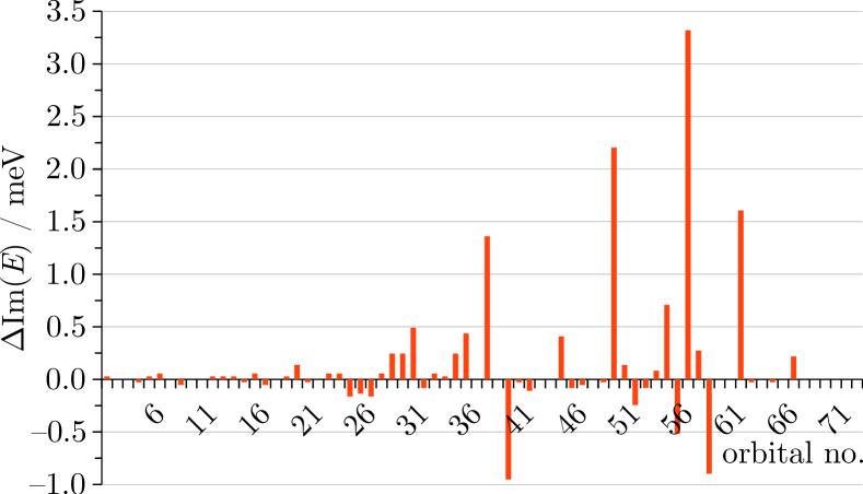
Figure 5: Contributions of virtual orbitals of a₁ symmetry to the CBF-CCSD decay width of the $2\text{a}_{1}2\text{a}_{1}$ channel of H₂O⁺ (1s^-1). The analysis was done with the aug-cc-pCVTZ (5sp) basis and 2 complex-scaled s, p, and d shells on all atoms.

IV.3 Dinitrogen

As a second example, we examined the core-ionized states of the nitrogen molecule. The neutral ground state has the electronic configuration $1\upsigma_{g}^{2}1\upsigma_{u}^{2}2\upsigma_{g}^{2}2\upsigma_{u}^{2}1\uppi_{g}^{4}3\upsigma_{g}^{2}$. Two core-ionized states ${}^{2}\Sigma_{g}^{+}$ and ${}^{2}\Sigma_{u}^{+}$ can be distinguished depending on whether an electron is removed from the 1$\upsigma_{g}$ or the 1$\upsigma_{u}$ orbital. The energy splitting between these two orbitals is very small (ca. 80 meV in an RHF calculation) so that one expects the two core-ionized states to overlap in terms of their widths. This aspect has been discussed elsewhere before.Lindle et al. (1984); Hergenhahn et al. (2001); Semenov et al. (2005); Sorensen et al. (2008)

Table 9: Energies and half-widths of the ${}^{2}\Sigma_{g}^{+}$ and ${}^{2}\Sigma_{u}^{+}$ core-ionized states of N${}_{2}^{+}$ computed with CBF-EOMIP-CCSD. Energies in eV. Half-widths in meV.

Unscaled	Complex-
basis set	scaled shells${}^{\text{a}}$	$\theta_{\text{opt}}/^{\circ}$	$\text{Re}(E)$	$\text{Im}(E)$
${}^{2}\Sigma_{g}^{+}$ state
aug-cc-pCV5Z	3$\times$(spd)	18	411.28	$-$55
aug-cc-pCVQZ	3$\times$(spd)	12	411.29	$-$50
aug-cc-pCVTZ	3$\times$(spd)	8	411.24	$-$58
aug-cc-pCVTZ (5sp)	3$\times$(spd)	22	411.24	$-$63
Experiment			409.96${}^{\text{b}}$	$-$58c
${}^{2}\Sigma_{u}^{+}$ state
aug-cc-pCV5Z	3$\times$(spd)	25	411.19	$-$55
aug-cc-pCVQZ	3$\times$(spd)	12	411.19	$-$53
aug-cc-pCVTZ	3$\times$(spd)	8	411.14	$-$54
aug-cc-pCVTZ (5sp)	3$\times$(spd)	19	411.14	$-$63
Experiment			409.88${}^{\text{b}}$	$-$62${}^{\text{c}}$

Our CBF-EOMIP-CCSD results in Tab. 9 confirm that the two resonances overlap indeed. The widths of both states are computed to be ca. 120 meV in good agreement with experimental values,Semenov et al. (2005) whereas the energy gap is 100 meV. The experimental value for the energy gap is 80 meVSorensen et al. (2008) meaning the overlap is somewhat more pronounced. The ionization energies themselves are again systematically overestimated similar to what we found for neon and water.

We found that it is necessary to scale three s, p, and d shells in order to obtain converged results for the decay widths. When doing so, a standard basis set such as aug-cc-pCVTZ is already able to capture most of the total decay width. In contrast, when scaling only two shells, which works well for water, the decay widths deviate by more than 20% from the experimental values and no basis set convergence is observed when going from aug-cc-pCVTZ to aug-cc-pCV5Z. This is documented in the Supporting Information. One may speculate that the need to scale a third shell is related to the presence of two heavy nuclei in N₂. The target states of Auger decay are presumably not well described when only two shells are complex scaled.

A further aspect of the core-ionized states of N₂ is vibrational progression resulting from the dependence of the energy and decay width on the bond length.Lindle et al. (1984); Hergenhahn et al. (2001); Semenov et al. (2005); Sorensen et al. (2008) The experimental values for $\Gamma/2$ in Tab. 9 are vibrationally unresolved while our theoretical results in the same table are computed at $R$(NN)= 1.1 Å and do not account for any vibrational effects.

To get an estimate of the dependence of $E$ and $\Gamma$ on the bond length, we recomputed these quantities in the range $R$(NN) = 1.00–1.20 Å. The results in Fig. 6 illustrate that the widths of both resonances depend only weakly on $R$(NN), only a slight increase is observed at shorter bond lengths. This finding is consistent with the core orbitals not participating in the bond between the two nitrogen atoms and can be contrasted with valence resonances such as the ${}^{2}\Pi_{g}$ state of N${}_{2}^{-}$ where $\Gamma$ depends strongly on the molecular structure.Jagau, Bravaya, and Krylov (2017) In contrast to the decay width, the ionization energies change by ca. 1 eV in the range of $R$(NN) that we investigated. Also, the energy gap between the two states decreases at stretched bond lengths.

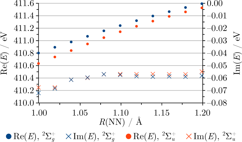
Figure 6: Dependence of energies and decay widths of the ${}^{2}\Sigma_{g}^{+}$ and ${}^{2}\Sigma_{u}^{+}$ core-ionized states of N${}_{2}^{+}$ on the NN bond distance computed with CBF-EOMIP-CCSD/aug-cc-pCVTZ (5sp) and three complex-scaled s, p, and d shells on each atom.

IV.4 Benzene

To demonstrate the applicability of our approach to larger molecules, we investigated the lowest core-ionized state of benzene using CBF-EOMIP-CCSD and the 6-311+G(3df) (unc.), aug-cc-pCVTZ, and aug-cc-pCVTZ (5sp) basis sets. We placed 2 or 3 complex-scaled s, p, and d shells at all carbon atoms. The resulting numbers of basis functions and compute times as well as results of all computations can be found in Tab. 10.

Table 10: Energies and half-widths of the ${}^{2}\text{A}_{1g}$ core-ionized state of C₆H${}_{6}^{+}$ computed with CBF-EOMIP-CCSD.

Unscaled	6-311+G(3df)	aug-cc-	aug-cc-
basis set	(unc.)	pCVTZ	pCVTZ (5sp)
Complex-	2$\times$(spd)	3$\times$(spd)
scaled shells	at all C atoms	at all C atoms
Basis functions	450	654	798
Compute time${}^{\text{a}}$/h	4.6	16.4	45.8
$\theta_{\text{opt}}$ / ∘	18	8	13
$\text{d}E/\text{d}\theta$/Hartree/∘	$3.4\cdot 10^{-5}$	$1.5\cdot 10^{-4}$	$2.0\cdot 10^{-6}$
Re($E$)/eV	291.88	291.98	291.99
Im($E$)/meV	$-$58.5	$-$37.8	$-$41.6

The results exhibit a similar trend as those for N₂: aug-cc-pCVTZ and aug-cc-pCVTZ (5sp) yield almost identical ionization energies, again somewhat higher than the experimental value of 290.42 eVRennie et al. (2000). The decay widths differ by about 10 % from each other, which is also reminiscent of N₂, whereas the 6-311+G(3df) (unc.) basis produces a 50% larger width. Given that aug-cc-pCVTZ (5sp) yields the smallest value for $\text{d}E/\text{d}\theta$ and also led to the best agreement with reference values for the other examples discussed in the previous sections, we conclude that our final result for the Auger decay width of benzene is 83 meV. This value is in good agreement with the decay width of core-ionized methane;Skomorowski and Krylov (2021b) a rigorous assessment is, however, difficult because no experimental or theoretical values are available for the decay width of benzene although the Auger spectrum has been studied theoretically before.Tarantelli et al. (1987)

We note that it takes almost two days on a state-of-the-art 16-core machine to compute one complex EOMIP-CCSD energy in the aug-cc-pCVTZ (5sp) basis set (798 basis functions). Since 10 to 20 computations are necessary to determine the optimal scaling angle, this illustrates the size of the calculations that are possible with our current hardware.

V Conclusions and Outlook

We have shown how to compute total and partial Auger decay widths in the framework of complex-variable coupled-cluster theory. We discussed the evaluation of these quantities based on CCSD and EOMIP-CCSD wave functions using complex scaling of the Hamiltonian or, alternatively, of parts of the basis set. The latter approach extends the formalism of complex scaling to molecular resonances and, in addition, is superior in terms of numerical performance. This manifests itself in smaller decay widths of bound states, whose lifetime is infinite in the complete basis-set limit, and faster convergence of the HF and CCSD equations.

In complex-variable methods, the total decay width is obtained as imaginary part of the eigenvalue of a non-Hermitian Hamiltonian without the need to make any assumption about the wave function of the emitted electron. Our applications of complex-scaled basis functions to core-ionized states of Ne, H₂O, and N₂ demonstrated excellent agreement for total Auger decay widths with experimental and previous theoretical investigations with errors of only a few percent. We also reported the first value for the Auger decay width of core-ionized C₆H₆; the result is in good agreement with the Auger decay width of CH₄. A caveat regarding the accuracy of our results is that the basis-set requirements of complex-scaled calculations on core-vacant states are not yet fully explored. While two complex-scaled s, p, and d shells appear to be sufficient for describing Auger decay of Ne and H₂O, three sets are required for N₂.

We gained access to partial decay widths and branching ratios by decomposing the imaginary part of the CCSD or EOM-CCSD energy, respectively, in terms of individual amplitudes. This analysis illustrated that –as one would expect– the largest share of the decay width is delivered by those excitations, which are removed from the wave function in CVS methods. However, other excitations yield non-negligible contributions in EOMIP-CCSD, which complicates the analysis. In addition, there is a nonadditivity of the partial widths in our approach. Overall, we found that partial widths computed with $\Delta$CCSD are more reliable than those computed with EOMIP-CCSD.

The analysis of the imaginary part of the energy also gave insight into the requirements towards the basis set that the treatment of Auger decay poses. We found that it is sufficient to add 1–3 complex-scaled s, p, and d shells to an unscaled basis set that is suitable for the treatment of core-vacant states. The exponents of these extra shells need to be chosen carefully to capture the decaying character of a core-ionized state, but their values can be estimated from the energy of the emitted Auger electron. This means in effect that the complex-scaled shells have exponents in the range 1–10, which is in contrast to resonances that decay by emission of slow electrons, where extra diffuse shells are pivotal.

We consider our work a critical extension of CC theory for core-vacant states. In our view, the prospects for applying complex-variable methods to core-vacant states are rather bright. A particular strength of complex-variable methods is that they offer a unified treatment of different types of resonances and are equally applicable to Feshbach and shape resonances. The latter are relevant for low-energy electron attachment and tunnel ionization but also of interest in the context of X-ray spectroscopy.Sorensen et al. (2008) Alternative approaches for decaying states based on Fano’s theory work well for Feshbach resonances but face problems when applied to shape resonances. Their main advantage is lower computational cost; all relevant states are modeled as bound states and the decay is treated separately afterwards. One may speculate that methods based on Fano’s theory will emerge as superior for cases where the partition of the Hilbert space into a bound and a continuum part poses no problems. The main advantage of complex-scaled calculations, in contrast, is that they can be used in a black-box fashion because no explicit treatment of the continuum is necessary. The need for the optimization of the scaling angle, however, increases the computational cost. In this work, we usually found 10 calculations to be sufficient to determine it to sufficient accuracy. The largest calculation that we carried out comprised 798 basis functions.

In order to treat larger systems with complex-scaled methods, two strategies appear worthwhile to pursue: On the one hand, our approach can be easily adapted to related electronic-structure methods such as the second-order CC modelChristiansen, Koch, and Jørgensen (1995) or algebraic diagrammatic construction (ADC) schemesSchirmer (1982) which entail lower computational cost. On the other hand, complex-variable CCSD and EOMIP-CCSD can be combined with quantum embedding.Parravicini and Jagau (2021)

We add that our approach to extract partial widths from complex-variable calculations is not specific to Auger decay. In complex systems, not only Auger decay is of interest but also related non-local phenomena such as intermolecular Coulombic decay and electron-transfer mediated decay. We anticipate that our approach can be applied to these processes as well. Finally, we mention that nuclear motion will need to be taken into account in order to model the vibrational progression observed in experimental Auger electron spectra.

Supplementary Material

See supplementary material for molecular structures, details about the basis sets used in our calculations as well as further results.

Data Availability Statement

The data that support the findings of this study are available within the article and its supplementary material.

Author Declarations

The authors have no conflicts to disclose.

References

- Agarwal (2013) B. K. Agarwal, X-ray spectroscopy: an introduction (Springer, 2013).
- Norman and Dreuw (2018) P. Norman and A. Dreuw, “Simulating X-ray spectroscopies and calculating core-excited states of molecules,” Chem. Rev. 118, 7208–7248 (2018).
- Zimmermann et al. (2020) P. Zimmermann, S. Peredkov, P. M. Abdala, S. DeBeer, M. Tromp, C. Müller, and J. A. van Bokhoven, “Modern X-ray spectroscopy: XAS and XES in the laboratory,” Coord. Chem. Rev. 423, 213466 (2020).
- Meitner (1922) L. Meitner, “Über die -Strahl-Spektra und ihren Zusammenhang mit der -Strahlung,” Z. Phys. 11, 35 (1922).
- Auger (1923) P. Auger, “Sur les rayons secondaires produits dans un gaz par des rayons X.” CR Acad. Sci. (F) 177, 169 (1923).
- Brown et al. (1980) G. S. Brown, M. H. Chen, B. Crasemann, and G. E. Ice, “Observation of the Auger resonant Raman effect,” Phys. Rev. Lett. 45, 1937–1940 (1980).
- Armen et al. (2000) G. B. Armen, H. Aksela, T. Åberg, and S. Aksela, “The resonant Auger effect,” J. Phys. B-At. Mol. Opt. 33, R49–R92 (2000).
- Carlson and Krause (1965) T. A. Carlson and M. O. Krause, “Experimental evidence for double electron emission in an Auger process,” Phys. Rev. Lett. 14, 390–392 (1965).
- Müller et al. (2015) A. Müller, A. Borovik, T. Buhr, J. Hellhund, K. Holste, A. L. D. Kilcoyne, S. Klumpp, M. Martins, S. Ricz, J. Viefhaus, and S. Schippers, “Observation of a four-electron auger process in near--edge photoionization of singly charged carbon ions,” Phys. Rev. Lett. 114, 013002 (2015).
- Lee et al. (1993) I. Lee, R. Wehlitz, U. Becker, and M. Ya Amusia, “Evidence for a new class of many-electron auger transitions in atoms,” J. Phys. B-At. Mol. Opt. 26, L41–L45 (1993).
- Feifel et al. (2016) R. Feifel, J. H. D. Eland, R. J. Squibb, M. Mucke, S. Zagorodskikh, P. Linusson, F. Tarantelli, P. Kolorenč, and V. Averbukh, “Ultrafast molecular three-electron auger decay,” Phys. Rev. Lett. 116, 073001 (2016).
- Cederbaum, Zobeley, and Tarantelli (1997) L. S. Cederbaum, J. Zobeley, and F. Tarantelli, “Giant intermolecular decay and fragmentation of clusters,” Phys. Rev. Lett. 79, 4778–4781 (1997).
- Jahnke et al. (2020) T. Jahnke, U. Hergenhahn, B. Winter, R. Dörner, U. Frühling, P. V. Demekhin, K. Gokhberg, L. S. Cederbaum, A. Ehresmann, A. Knie, and A. Dreuw, “Interatomic and intermolecular Coulombic decay,” Chem. Rev. 120, 11295–11369 (2020).
- Zobeley, Santra, and Cederbaum (2001) J. Zobeley, R. Santra, and L. S. Cederbaum, “Electronic decay in weakly bound heteroclusters: Energy transfer versus electron transfer,” J. Chem. Phys. 115, 5076–5088 (2001).
- Manne and Ågren (1985) R. Manne and H. Ågren, “Auger transition amplitudes from general many-electron wavefunctions,” Chem. Phys. 93, 201–208 (1985).
- Zähringer, Meyer, and Cederbaum (1992a) K. Zähringer, H.-D. Meyer, and L. S. Cederbaum, “Molecular scattering wave functions for Auger decay rates: The Auger spectrum of hydrogen fluoride,” Phys. Rev. A 45, 318–328 (1992a).
- Zähringer, Meyer, and Cederbaum (1992b) K. Zähringer, H.-D. Meyer, and L. S. Cederbaum, “Angularly resolved Auger rates of LiF and HF,” Phys. Rev. A 46, 5643–5652 (1992b).
- Tarantelli, Sgamellotti, and Cederbaum (1994) F. Tarantelli, A. Sgamellotti, and L. S. Cederbaum, “The calculation of molecular Auger spectra,” J. Electron Spectrosc. 68, 297–312 (1994).
- Yarzhemsky and Sgamellotti (2002) V. G. Yarzhemsky and A. Sgamellotti, “Auger rates of second-row atoms calculated by many-body perturbation theory,” J. Electron Spectrosc. Relat. Phenom. 125, 13–24 (2002).
- Kolorenc and Averbukh (2011) P. Kolorenc and V. Averbukh, “K-shell Auger lifetime variation in doubly ionized Ne and first row hydrides,” J. Chem. Phys. 135, 134314 (2011).
- Inhester et al. (2012) L. Inhester, C. F. Burmeister, G. Groenhof, and H. Grubmüller, “Auger spectrum of a water molecule after single and double core ionization,” J. Chem. Phys. 136, 144304 (2012).
- Inhester et al. (2014) L. Inhester, C. F. Burmeister, G. Groenhof, and H. Grubmüller, “Erratum: “Auger spectrum of a water molecule after single and double core ionization” [J. Chem. Phys. 136, 144304 (2012)],” J. Chem. Phys. 141, 069904 (2014).
- Skomorowski and Krylov (2021a) W. Skomorowski and A. I. Krylov, “Feshbach–Fano approach for calculation of Auger decay rates using equation-of-motion coupled-cluster wave functions. I. Theory and implementation,” J. Chem. Phys. 154, 084124 (2021a).
- Skomorowski and Krylov (2021b) W. Skomorowski and A. I. Krylov, “Feshbach–Fano approach for calculation of Auger decay rates using equation-of-motion coupled-cluster wave functions. II. Numerical examples and benchmarks,” J. Chem. Phys. 154, 084125 (2021b).
- Moiseyev (2011) N. Moiseyev, Non-Hermitian Quantum Mechanics (Cambridge University Press, 2011).
- Jagau, Bravaya, and Krylov (2017) T.-C. Jagau, K. B. Bravaya, and A. I. Krylov, “Extending quantum chemistry of bound states to electronic resonances,” Annu. Rev. Phys. Chem. 68, 525–553 (2017).
- Cederbaum, Domcke, and Schirmer (1980) L. S. Cederbaum, W. Domcke, and J. Schirmer, “Many-body theory of core holes,” Phys. Rev. A 22, 206–222 (1980).
- Coriani and Koch (2015) S. Coriani and H. Koch, “Communication: X-ray absorption spectra and core-ionization potentials within a core-valence separated coupled cluster framework,” J. Chem. Phys. 143, 181103 (2015).
- Vidal et al. (2019) M. L. Vidal, X. Feng, E. Epifanovsky, A. I. Krylov, and S. Coriani, “New and efficient equation-of-motion coupled-cluster framework for core-excited and core-ionized states,” J. Chem. Theory Comput. 15, 3117–3133 (2019).
- Fransson et al. (2021) T. Fransson, I. E. Brumboiu, M. L. Vidal, P. Norman, S. Coriani, and A. Dreuw, “XABOOM: an X-ray absorption benchmark of organic molecules based on carbon, nitrogen, and oxygen 1s → * transitions,” J. Chem. Theory Comput. 17, 1618–1637 (2021).
- García et al. (2009) J. García, T. R. Kallman, M. Witthoeft, E. Behar, C. Mendoza, P. Palmeri, P. Quinet, M. A. Bautista, and M. Klapisch, “Nitrogen K-shell photoabsorption,” Astrophys. J. Suppl. S. 185, 477–485 (2009).
- Gorczyca (2000) T. W. Gorczyca, “Auger decay of the photoexcited Rydberg series in neon,” Phys. Rev. A 61, 024702 (2000).
- Fano (1961) U. Fano, “Effects of configuration interaction on intensities and phase shifts,” Phys. Rev. 124, 1866–1878 (1961).
- Feshbach (1962) H. Feshbach, “A unified theory of nuclear reactions. II,” Ann. Phys. (N.Y.) 19, 287–313 (1962).
- Langhoff and Corcoran (1974) P. W. Langhoff and C. T. Corcoran, “Stieltjes imaging of photoabsorption and dispersion profiles,” J. Chem. Phys. 61, 146–159 (1974).
- Carravetta and Ågren (1987) V. Carravetta and H. Ågren, “Stieltjes imaging method for molecular Auger transition rates: Application to the Auger spectrum of water,” Phys. Rev. A 35, 1022–1032 (1987).
- Averbukh and Cederbaum (2005) V. Averbukh and L. S. Cederbaum, “Ab initio calculation of interatomic decay rates by a combination of the Fano ansatz, Green’s-function methods, and the Stieltjes imaging technique,” J. Chem. Phys. 123, 204107 (2005).
- Kolorenč and Averbukh (2020) P. Kolorenč and V. Averbukh, “Fano-ADC(2,2) method for electronic decay rates,” J. Chem. Phys. 152, 214107 (2020).
- Schirmer (1982) J. Schirmer, “Beyond the random-phase approximation: A new approximation scheme for the polarization propagator,” Phys. Rev. A 26, 2395–2416 (1982).
- Aguilar and Combes (1971) J. Aguilar and J.-M. Combes, “A class of analytic perturbations for one-body Schrödinger Hamiltonians,” Commun. Math. Phys. 22, 269–279 (1971).
- Balslev and Combes (1971) E. Balslev and J.-M. Combes, “Spectral properties of many-body Schrödinger operators with dilatation-analytic interactions,” Commun. Math. Phys. 22, 280–294 (1971).
- McCurdy and Rescigno (1978) C. W. McCurdy and T. N. Rescigno, “Extension of the method of complex basis functions to molecular resonances,” Phys. Rev. Lett. 41, 1364–1368 (1978).
- Moiseyev and Corcoran (1979) N. Moiseyev and C. Corcoran, “Autoionizing states of and using the complex-scaling method,” Phys. Rev. A 20, 814–817 (1979).
- Bravaya et al. (2013) K. B. Bravaya, D. Zuev, E. Epifanovsky, and A. I. Krylov, “Complex-scaled equation-of-motion coupled-cluster method with single and double substitutions for autoionizing excited states: Theory, implementation, and examples,” J. Chem. Phys. 138, 124106 (2013).
- Jagau et al. (2014) T.-C. Jagau, D. Zuev, K. B. Bravaya, E. Epifanovsky, and A. I. Krylov, “A fresh look at resonances and complex absorbing potentials: Density matrix-based approach,” J. Phys. Chem. Lett. 5, 310–315 (2014).
- Zuev et al. (2014) D. Zuev, T.-C. Jagau, K. B. Bravaya, E. Epifanovsky, Y. Shao, E. Sundstrom, M. Head-Gordon, and A. I. Krylov, “Complex absorbing potentials within EOM-CC family of methods: Theory, implementation, and benchmarks,” J. Chem. Phys. 141, 024102 (2014).
- White, Head-Gordon, and McCurdy (2015) A. F. White, M. Head-Gordon, and C. W. McCurdy, “Complex basis functions revisited: Implementation with applications to carbon tetrafluoride and aromatic N-containing heterocycles within the static-exchange approximation,” J. Chem. Phys. 142, 054103 (2015).
- White, McCurdy, and Head-Gordon (2015) A. F. White, C. W. McCurdy, and M. Head-Gordon, “Restricted and unrestricted non-Hermitian Hartree-Fock: Theory, practical considerations, and applications to metastable molecular anions,” J. Chem. Phys. 143, 074103 (2015).
- White et al. (2017) A. F. White, E. Epifanovsky, C. W. McCurdy, and M. Head-Gordon, “Second order Møller-Plesset and coupled cluster singles and doubles methods with complex basis functions for resonances in electron-molecule scattering,” J. Chem. Phys. 146, 234107 (2017).
- Moiseyev, Certain, and Weinhold (1978) N. Moiseyev, P. R. Certain, and F. Weinhold, “Resonance properties of complex-rotated Hamiltonians,” Mol. Phys. 36, 1613–1630 (1978).
- Zhang and Yeager (2012a) S. B. Zhang and D. L. Yeager, “A complex scaled multi-reference configuration interaction method to study Li and Li-like cations (Be, B, C, N, O) Auger resonances and ,” J. Mol. Struct. 1023, 96–100 (2012a).
- Zhang and Yeager (2012b) S. B. Zhang and D. L. Yeager, “Complex-scaled multireference configuration-interaction method to study Be and Be-like cations’ (B, C, N, O, Mg) Auger resonances ,” Phys. Rev. A 85, 032515 (2012b).
- Peng et al. (2016) Y.-G. Peng, Y. Wu, L.-F. Zhu, S. B. Zhang, J.-G. Wang, H.-P. Liebermann, and R. J. Buenker, “Complex multireference configuration interaction calculations for the K-vacancy Auger states of (q = 2-5) ions,” J. Chem. Phys. 144, 054306 (2016).
- Jagau (2018) T.-C. Jagau, “Coupled-cluster treatment of molecular strong-field ionization,” J. Chem. Phys. 148, 204102 (2018).
- Thompson, Ochsenfeld, and Jagau (2019) T. H. Thompson, C. Ochsenfeld, and T.-C. Jagau, “A Schwarz inequality for complex basis function methods in non-Hermitian quantum chemistry,” J. Chem. Phys. 151, 184104 (2019).
- Hernández Vera and Jagau (2019) M. Hernández Vera and T.-C. Jagau, “Resolution-of-the-identity approximation for complex-scaled basis functions,” J. Chem. Phys. 151, 111101 (2019).
- Hernández Vera and Jagau (2020) M. Hernández Vera and T.-C. Jagau, “Resolution-of-the-identity second-order Møller–Plesset perturbation theory with complex basis functions: Benchmark calculations and applications to strong-field ionization of polyacenes,” J. Chem. Phys. 152, 174103 (2020).
- Ghosh, Pal, and Vaval (2013) A. Ghosh, S. Pal, and N. Vaval, “Study of interatomic Coulombic decay of Ne(H2O)n ( = 1,3) clusters using equation-of-motion coupled-cluster method,” J. Chem. Phys. 139, 064112 (2013).
- Ghosh, Pal, and Vaval (2015) A. Ghosh, S. Pal, and N. Vaval, “Lifetime of inner-shell hole states of Ar (2p) and Kr (3d) using equation-of-motion coupled cluster method,” J. Chem. Phys. 143, 024305 (2015).
- Ghosh, Vaval, and Pal (2017) A. Ghosh, N. Vaval, and S. Pal, “Auger decay rates of core hole states using equation of motion coupled cluster method,” Chem. Phys. 482, 160–164 (2017).
- Moiseyev (1998) N. Moiseyev, “Derivations of universal exact complex absorption potentials by the generalized complex coordinate method,” J. Phys. B-At. Mol. Opt. 31, 1431–1441 (1998).
- Riss and Meyer (1993) U. V. Riss and H. D. Meyer, “Calculation of resonance energies and widths using the complex absorbing potential method,” J. Phys. B-At. Mol. Opt. 26, 4503–4536 (1993).
- Riss and Meyer (1998) U. V. Riss and H.-D. Meyer, “The transformative complex absorbing potential method: a bridge between complex absorbing potentials and smooth exterior scaling,” J. Phys. B-At. Mol. Opt. 31, 2279–2304 (1998).
- Čížek (1966) J. Čížek, “On the correlation problem in atomic and molecular systems. calculation of wavefunction components in Ursell-type expansion using quantum-field theoretical methods,” J. Chem. Phys. 45, 4256–4266 (1966).
- Čížek (1969) J. Čížek, “On the use of the cluster expansion and the technique of diagrams in calculations of correlation effects in atoms and molecules,” Adv. Chem. Phys. 14, 35–89 (1969).
- Shavitt and Bartlett (2009) I. Shavitt and R. J. Bartlett, Many-Body Methods in Chemistry and Physics: MBPT and Coupled-Cluster Theory (Cambridge University Press, 2009).
- Emrich (1981) K. Emrich, “An extension of the coupled cluster formalism to excited states (I),” Nucl. Phys. A 351, 379–396 (1981).
- Sekino and Bartlett (1984) H. Sekino and R. J. Bartlett, “A linear response, coupled-cluster theory for excitation energy,” Int. J. Quantum Chem. 26, 255–265 (1984).
- Stanton and Bartlett (1993) J. F. Stanton and R. J. Bartlett, “The equation of motion coupled-cluster method. A systematic biorthogonal approach to molecular excitation energies, transition probabilities, and excited state properties,” J. Chem. Phys. 98, 7029–7039 (1993).
- Nooijen and Snijders (1993) M. Nooijen and J. G. Snijders, “Coupled cluster Green’s function method: Working equations and applications,” Int. J. Quantum Chem. 48, 15–48 (1993).
- Stanton and Gauss (1994) J. F. Stanton and J. Gauss, “Analytic energy derivatives for ionized states described by the equation-of-motion coupled cluster method,” J. Chem. Phys. 101, 8938–8944 (1994).
- Zheng and Cheng (2019) X. Zheng and L. Cheng, “Performance of delta-coupled-cluster methods for calculations of core-ionization energies of first-row elements,” J. Chem. Theory Comput. 15, 4945–4955 (2019).
- Park, Perera, and Bartlett (2019) Y. C. Park, A. Perera, and R. J. Bartlett, “Equation of motion coupled-cluster for core excitation spectra: Two complementary approaches,” J. Chem. Phys. 151, 164117 (2019).
- Frati et al. (2019) F. Frati, F. de Groot, J. Cerezo, F. Santoro, L. Cheng, R. Faber, and S. Coriani, “Coupled cluster study of the x-ray absorption spectra of formaldehyde derivatives at the oxygen, carbon, and fluorine K-edges,” J. Chem. Phys. 151, 064107 (2019).
- Liu et al. (2019) J. Liu, D. Matthews, S. Coriani, and L. Cheng, “Benchmark calculations of K-edge ionization energies for first-row elements using scalar-relativistic core–valence-separated equation-of-motion coupled-cluster methods,” J. Chem. Theory Comput. 15, 1642–1651 (2019).
- Nanda et al. (2020) K. D. Nanda, M. L. Vidal, R. Faber, S. Coriani, and A. I. Krylov, “How to stay out of trouble in RIXS calculations within equation-of-motion coupled-cluster damped response theory? Safe hitchhiking in the excitation manifold by means of core–valence separation,” Phys. Chem. Chem. Phys. 22, 2629–2641 (2020).
- Vidal et al. (2020) M. L. Vidal, P. Pokhilko, A. I. Krylov, and S. Coriani, “Equation-of-motion coupled-cluster theory to model L-edge X-ray absorption and photoelectron spectra,” J. Phys. Chem. Lett. 11, 8314–8321 (2020).
- Vidal, Krylov, and Coriani (2020) M. L. Vidal, A. I. Krylov, and S. Coriani, “Dyson orbitals within the fc-CVS-EOM-CCSD framework: theory and application to X-ray photoelectron spectroscopy of ground and excited states,” Phys. Chem. Chem. Phys. 22, 2693–2703 (2020).
- Matthews (2020) D. A. Matthews, “EOM-CC methods with approximate triple excitations applied to core excitation and ionisation energies,” Mol. Phys. 118, e1771448 (2020).
- Besley and Asmuruf (2010) N. A. Besley and F. A. Asmuruf, “Time-dependent density functional theory calculations of the spectroscopy of core electrons,” Phys. Chem. Chem. Phys. 12, 12024–12039 (2010).
- Besley, Gilbert, and Gill (2009) N. A. Besley, A. T. B. Gilbert, and P. M. W. Gill, “Self-consistent-field calculations of core excited states,” J. Chem. Phys. 130, 124308 (2009).
- Wenzel, Wormit, and Dreuw (2014a) J. Wenzel, M. Wormit, and A. Dreuw, “Calculating core-level excitations and X-ray absorption spectra of medium-sized closed-shell molecules with the algebraic-diagrammatic construction scheme for the polarization propagator,” J. Comput. Chem. 35, 1900 (2014a).
- Wenzel, Wormit, and Dreuw (2014b) J. Wenzel, M. Wormit, and A. Dreuw, “Calculating X-ray absorption spectra of open-shell molecules with the unrestricted algebraic-diagrammatic construction scheme for the polarization propagator,” J. Chem. Theory Comput. 10, 4583 (2014b).
- Wenzel et al. (2015) J. Wenzel, A. Holzer, M. Wormit, and A. Dreuw, “Analysis and comparison of cvs-adc approaches up to third order for the calculation of core-excited states,” J. Chem. Phys. 142, 214104 (2015).
- Simon (1979) B. Simon, “The definition of molecular resonance curves by the method of exterior complex scaling,” Physics Letters A 71, 211 (1979).
- Hazi and Taylor (1970) A. U. Hazi and H. S. Taylor, “Stabilization method of calculating resonance energies: Model problem,” Phys. Rev. A 1, 1109–1120 (1970).
- Taylor and Hazi (1976) H. S. Taylor and A. U. Hazi, “Comment on the stabilization method: Variational calculation of the resonance width,” Phys. Rev. A 14, 2071–2074 (1976).
- Epifanovsky et al. (2021) E. Epifanovsky, A. T. B. Gilbert, X. Feng, J. Lee, Y. Mao, N. Mardirossian, P. Pokhilko, A. F. White, M. P. Coons, A. L. Dempwolff, Z. Gan, D. Hait, P. R. Horn, L. D. Jacobson, I. Kaliman, J. Kussmann, A. W. Lange, K. U. Lao, D. S. Levine, J. Liu, S. C. McKenzie, A. F. Morrison, K. D. Nanda, F. Plasser, D. R. Rehn, M. L. Vidal, Z.-Q. You, Y. Zhu, B. Alam, B. J. Albrecht, A. Aldossary, E. Alguire, J. H. Andersen, V. Athavale, D. Barton, K. Begam, A. Behn, N. Bellonzi, Y. A. Bernard, E. J. Berquist, H. G. A. Burton, A. Carreras, K. Carter-Fenk, R. Chakraborty, A. D. Chien, K. D. Closser, V. Cofer-Shabica, S. Dasgupta, M. de Wergifosse, J. Deng, M. Diedenhofen, H. Do, S. Ehlert, P.-T. Fang, S. Fatehi, Q. Feng, T. Friedhoff, J. Gayvert, Q. Ge, G. Gidofalvi, M. Goldey, J. Gomes, C. E. González-Espinoza, S. Gulania, A. O. Gunina, M. W. D. Hanson-Heine, P. H. P. Harbach, A. Hauser, M. F. Herbst, M. H. Vera, M. Hodecker, Z. C. Holden, S. Houck, X. Huang, K. Hui, B. C. Huynh, M. Ivanov, Ádám Jász, H. Ji, H. Jiang, B. Kaduk, S. Kähler, K. Khistyaev, J. Kim, G. Kis, P. Klunzinger, Z. Koczor-Benda, J. H. Koh, D. Kosenkov, L. Koulias, T. Kowalczyk, C. M. Krauter, K. Kue, A. Kunitsa, T. Kus, I. Ladjánszki, A. Landau, K. V. Lawler, D. Lefrancois, S. Lehtola, R. R. Li, Y.-P. Li, J. Liang, M. Liebenthal, H.-H. Lin, Y.-S. Lin, F. Liu, K.-Y. Liu, M. Loipersberger, A. Luenser, A. Manjanath, P. Manohar, E. Mansoor, S. F. Manzer, S.-P. Mao, A. V. Marenich, T. Markovich, S. Mason, S. A. Maurer, P. F. McLaughlin, M. F. S. J. Menger, J.-M. Mewes, S. A. Mewes, P. Morgante, J. W. Mullinax, K. J. Oosterbaan, G. Paran, A. C. Paul, S. K. Paul, F. Pavošević, Z. Pei, S. Prager, E. I. Proynov, Ádám Rák, E. Ramos-Cordoba, B. Rana, A. E. Rask, A. Rettig, R. M. Richard, F. Rob, E. Rossomme, T. Scheele, M. Scheurer, M. Schneider, N. Sergueev, S. M. Sharada, W. Skomorowski, D. W. Small, C. J. Stein, Y.-C. Su, E. J. Sundstrom, Z. Tao, J. Thirman, G. J. Tornai, T. Tsuchimochi, N. M. Tubman, S. P. Veccham, O. Vydrov, J. Wenzel, J. Witte, A. Yamada, K. Yao, S. Yeganeh, S. R. Yost, A. Zech, I. Y. Zhang, X. Zhang, Y. Zhang, D. Zuev, A. Aspuru-Guzik, A. T. Bell, N. A. Besley, K. B. Bravaya, B. R. Brooks, D. Casanova, J.-D. Chai, S. Coriani, C. J. Cramer, G. Cserey, A. E. DePrince, R. A. DiStasio, A. Dreuw, B. D. Dunietz, T. R. Furlani, W. A. Goddard, S. Hammes-Schiffer, T. Head-Gordon, W. J. Hehre, C.-P. Hsu, T.-C. Jagau, Y. Jung, A. Klamt, J. Kong, D. S. Lambrecht, W. Liang, N. J. Mayhall, C. W. McCurdy, J. B. Neaton, C. Ochsenfeld, J. A. Parkhill, R. Peverati, V. A. Rassolov, Y. Shao, L. V. Slipchenko, T. Stauch, R. P. Steele, J. E. Subotnik, A. J. W. Thom, A. Tkatchenko, D. G. Truhlar, T. V. Voorhis, T. A. Wesolowski, K. B. Whaley, H. L. Woodcock, P. M. Zimmerman, S. Faraji, P. M. W. Gill, M. Head-Gordon, J. M. Herbert, and A. I. Krylov, “Software for the frontiers of quantum chemistry: An overview of developments in the Q-Chem 5 package,” J. Chem. Phys. 155, 084801 (2021).
- Howat et al. (1977) G. Howat, T. Åberg, O. Goscinski, S. C. Soong, C. P. Bhalla, and M. Ahmed, “Effect of interchannel interaction on the neon KLL auger transition rates,” Phys. Lett. A 60, 404–406 (1977).
- Albiez et al. (1990) A. Albiez, M. Thoma, W. Weber, and W. Mehlhorn, “ ionization in neon by electron impact in the range 1.5–50 keV: cross sections and alignment,” Z. Phys. D 16, 97–106 (1990).
- Coreno et al. (1999) M. Coreno, L. Avaldi, R. Camilloni, K. C. Prince, M. de Simone, J. Karvonen, R. Colle, and S. Simonucci, “Measurement and ab initio calculation of the Ne photoabsorption spectrum in the region of the K edge,” Phys. Rev. A 59, 2494–2497 (1999).
- Müller et al. (2017) A. Müller, D. Bernhardt, A. B. Jr., T. Buhr, J. Hellhund, K. Holste, A. L. D. Kilcoyne, S. Klumpp, M. Martins, S. Ricz, et al., “Photoionization of Ne atoms and Ne+ ions near the K edge: Precision spectroscopy and absolute cross-sections,” Astrophys. J. 836, 166 (2017).
- Colle and Simonucci (1993) R. Colle and S. Simonucci, “Multichannel resonance processes: Theory and application to the Auger spectra of the CO molecule,” Phys. Rev. A 48, 392–403 (1993).
- Colle and Simonucci (1990) R. Colle and S. Simonucci, “Interchannel coupling in Auger decay processes: Characterization of normal and satellite lines in the Auger electron spectrum of the LiF molecule,” Phys. Rev. A 42, 3913–3925 (1990).
- Sarangi et al. (2020) R. Sarangi, M. L. Vidal, S. Coriani, and A. I. Krylov, “On the basis set selection for calculations of core-level states: different strategies to balance cost and accuracy,” Mol. Phys. 118, e1769872 (2020).
- Sankari et al. (2003) R. Sankari, M. Ehara, H. Nakatsuji, Y. Senba, K. Hosokawa, H. Yoshida, A. De Fanis, Y. Tamenori, S. Aksela, and K. Ueda, “Vibrationally resolved O 1s photoelectron spectrum of water,” Chem. Phys. Lett. 380, 647–653 (2003).
- Ågren and Siegbahn (1980) H. Ågren and H. Siegbahn, “Semi-internal correlation in the Auger electron spectrum of H2O,” Chemical Physics Letters 69, 424–429 (1980).
- Moddeman et al. (1971) W. E. Moddeman, T. A. Carlson, M. O. Krause, B. P. Pullen, W. E. Bull, and G. K. Schweitzer, “Determination of the K—LL auger spectra of N2, O2, CO, NO, H2O, and CO2,” J. Chem. Phys. 55, 2317–2336 (1971).
- Lindle et al. (1984) D. W. Lindle, C. M. Truesdale, P. H. Kobrin, T. A. Ferrett, P. A. Heimann, U. Becker, H. G. Kerkhoff, and D. A. Shirley, “Nitrogen K-shell photoemission and Auger emission from N2 and NO,” J. Chem. Phys. 81, 5375–5378 (1984).
- Hergenhahn et al. (2001) U. Hergenhahn, O. Kugeler, A. Rüdel, E. E. Rennie, and A. M. Bradshaw, “Symmetry-selective observation of the N 1s shape resonance in N2,” J. Phys. Chem. A 105, 5704–5708 (2001).
- Semenov et al. (2005) S. K. Semenov, N. A. Cherepkov, M. Matsumoto, K. Fujiwara, K. Ueda, E. Kukk, F. Tahara, T. Sunami, H. Yoshida, T. Tanaka, et al., “Vibrationally resolved photoionization of the 1 and 1 shells of N2 molecule,” J. Phys. B–At. Mol. Opt. 39, 375–386 (2005).
- Sorensen et al. (2008) S. L. Sorensen, C. Miron, R. Feifel, M.-N. Piancastelli, O. Björneholm, and S. Svensson, “The influence of the resonance on the Auger decay of core-ionized molecular nitrogen,” Chem. Phys. Lett. 456, 1–6 (2008).
- Rennie et al. (2000) E. E. Rennie, B. Kempgens, H. M. Köppe, U. Hergenhahn, J. Feldhaus, B. S. Itchkawitz, A. L. D. Kilcoyne, A. Kivimäki, K. Maier, M. N. Piancastelli, M. Polcik, A. Rüdel, and A. M. Bradshaw, “A comprehensive photoabsorption, photoionization, and shake-up excitation study of the C 1s cross section of benzene,” J. Chem. Phys. 113, 7362–7375 (2000).
- Tarantelli et al. (1987) F. Tarantelli, A. Sgamellotti, L. S. Cederbaum, and J. Schirmer, “Theoretical investigation of many dicationic states and the Auger spectrum of benzene,” J. Chem. Phys. 86, 2201–2206 (1987).
- Christiansen, Koch, and Jørgensen (1995) O. Christiansen, H. Koch, and P. Jørgensen, “The second-order approximate coupled cluster singles and doubles model CC2,” Chem. Phys. Lett. 243, 409–418 (1995).
- Parravicini and Jagau (2021) V. Parravicini and T.-C. Jagau, “Embedded equation-of-motion coupled-cluster theory for electronic excitation, ionisation, electron attachment, and electronic resonances,” Mol. Phys. , e1943029 (2021).