Low-Precision Quantization for
Efficient Nearest Neighbor Search

Abstract.

Fast $k$-Nearest Neighbor search over real-valued vector spaces (Knn) is an important algorithmic task for information retrieval and recommendation systems. We present a method for using reduced precision to represent vectors through quantized integer values, enabling both a reduction in the memory overhead of indexing these vectors and faster distance computations at query time. While most traditional quantization techniques focus on minimizing the reconstruction error between a point and its uncompressed counterpart, we focus instead on preserving the behavior of the underlying distance metric. Furthermore, our quantization approach is applied at the implementation level and can be combined with existing Knn algorithms. Our experiments on both open source and proprietary datasets across multiple popular Knn frameworks validate that quantized distance metrics can reduce memory by $60\%$ and improve query throughput by $30\%$, while incurring only a $2\%$ reduction in recall.

1. Introduction

Knn search has become increasingly prevalent in machine learning applications and large-scale data systems for information retrieval (Huang et al., 2013) and recommendation systems targeting images (Amato and Falchi, 2010), audio (Kim et al., 2017), video (Wang et al., 2013), and textual data (Suchal and Návrat, 2010). The classical form of the problem is the following: given a query vector $\mathfrak{q}\in\mathbb{R}^{d}$, a distance metric $\phi$, and a set of vectors $\mathcal{I},$ where each $x\in\mathcal{I}$ is also in $\mathbb{R}^{d},$ find the set of $k$ vectors in $\mathcal{I}$ with the smallest distance to $\mathfrak{q}$.

Most methods for improving the performance of Knn focus on pruning the search space through the use of efficient data structures (Teflioudi and Gemulla, 2016; Li et al., 2017; Johnson et al., 2019; Garcia et al., 2008). Some methods also use compressed vector representations that trade a minimal loss of accuracy for orders of magnitude of compression (Han et al., 2015). This property allows these applications to scale to datasets which might not otherwise fit in physical memory. Common to all of these approaches, however, is that the computation of distances involves full-precision floating-point operations, often to the detriment of performance and memory overhead.

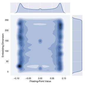
Figure 1. Distribution of values in a dataset of 100 million product embeddings derived from a large e-commerce catalog. We observe that the values comprising these embeddings cluster in a very narrow band.

In practice, we observe that Knn corpora found in both industry (Li et al., 2017) and open source datasets (Aumüller et al., 2020) are dramatically over-provisioned in terms of the range and precision that they can represent. For example, Figure 1 plots the distribution of feature values from a product embedding dataset used by a large e-commerce search engine. The data is highly-structured, with values observed exclusively in the range $(-.125,.125)$. The distribution is consistent across dimensions, with the majority of values (50%) observed in the narrow band $\pm(.125,.08)$.

This observation suggests a novel vector quantization method which focuses on feature-wise quantization. Given a corpus of vectors, we perform a data-driven analysis to determine the range of values that appear in practice and then quantize both the corpus and the distance function we intend to use into the lowest-precision integer domain that can capture the relative positions of the points in that set. As long as the quantization is distance preserving in the quantized space, the loss in recall is minimized. As a simple example, consider the following one-dimensional vectors (i.e. points) $\{1.23,2.34,3.09,1.4e7\}$. We can safely map these points into a smaller integer space of $\{1,2,3,4\}$ without considerable loss of recall in nearest-neighbors. The third point remains the nearest neighbor of the fourth, even after its value is altered by seven orders of magnitude.

This approach has two major consequences. First, by using a compact representation (say, int8), it is possible to reduce memory overhead and scale to larger datasets. This has direct implications on storage-specific design decisions and, hence, efficiency since an algorithm that stores vectors on disk will present significantly different performance properties than one which stores them in physical memory. Secondly, primitive computations involving integer data types can be more efficient than their floating-point counterparts. This implies that our approach can be combined with existing indexing-based KNN frameworks (Malkov and Yashunin, 2018; Johnson et al., 2019) as a mechanism for replacing full-precision vectors with compact integer alternatives, and obtaining reductions in runtime overhead.

2. Related Work

A large body of work in the Knn literature focuses on non-quantization-based approximate methods for performing inner product and nearest neighbor search. Locality sensitive hashing (Andoni et al., 2015; Shrivastava and Li, 2014), tree-based methods (Muja and Lowe, 2014; Dasgupta and Freund, 2008), and graph-based methods (Harwood and Drummond, 2016; Malkov and Yashunin, 2018) focus on achieving non-exhaustive search by partitioning the search space. Other work (He et al., 2013) focuses on learning short binary codes which can be searched using Hamming distances.

The seminal work which describes the application of quantization to Knn is product quantization (Jegou et al., 2010). In product quantization, the original vector space is decomposed into a Cartesian product of lower dimensional subspaces, and vector quantization is performed in each subspace independently. Vector quantization approximates a vector $x\in\mathbb{R}^{d}$ by finding the closest quantizer in a codebook $\mathbf{C}$

$$\phi_{VQ}(x;\mathbf{C})=\underset{c\in\left\{\mathbf{C}_{j}\right\}}{\operatorname{argmin}}\|x-c\|_{2}$$

where $\mathbf{C}\in\mathbb{R}^{d\times m}$ is a vector quantization codebook with $m$ codewords, and the $j$-th column $\mathbf{C}_{j}$ represents the $j$-th quantizer. This approach can be extended to $K$ subspaces. Numerous improvements have been proposed to this approach with the aim of reducing subspace dependencies (Ge et al., 2013; Norouzi and Fleet, 2013), including additive quantization (Babenko and Lempitsky, 2014), composite quantization  (Zhang et al., 2014, 2015) and stacked quantization (Martinez et al., 2014). Our approach is complementary to these approaches in the sense that one can either replace the original dataset with low-precision quantized vectors or use it after the codebook mapping step for calculating the distance computations at query time.

A closely related recent work is that of Guo et al. (2020), who proposed an anisotropic vector quantization scheme called ScaNN which, using an insight similar to ours, modifies the product quantization objective function to minimize the relative distance between vectors as opposed to the reconstruction distance. We note that our work and ScaNN are complementary. We make the same observations, but pursue them differently. ScaNN reformulates existing quantization approaches in terms of a new, relative distance-preserving optimization criteria. In this work, we do not make modifications to the underlying algorithms; instead, we modify them at the implementation level by utilizing efficient integer computations.

3. Low Precision Vector Quantization

3.1. Problem Formulation

We propose a quantization family $(\mathcal{Q},\phi)$ which is a combination of quantization function $\mathcal{Q}:\mathbb{R}^{d}\rightarrow\mathbb{Z}^{d}$ and distance function $\phi:\mathbb{Z}^{d}\times\mathbb{Z}^{d}\rightarrow\mathbb{Z}$. Following the notation in (Bachrach et al., 2014) we first introduce the notion of a search problem.

Definition 0.

A search problem $S(\mathcal{I},\mathcal{Q},d)$ consists of a set of $n$ items $\mathcal{I}=\left\{x_{1},x_{2},\ldots,x_{n}\right\},$ a set of queries $\mathcal{Q}$ and a search function $d:\mathcal{I}\times\mathcal{Q}\rightarrow\{1,2,\ldots,n\}$ such that the search function $d$ retrieves the index of an item in $\mathcal{I}$ for a given query $\mathfrak{q}\in\mathcal{Q}$.

In this work, we focus on the maximum inner product (MIP) search problem, namely the task of retrieving the items having the largest inner product with a query vector $q\in\mathbb{R}^{d}$. With this definition in hand, we can formalize the concept of a quantization between search problems, which is a preprocessing step designed to improve search efficiency.

Definition 0.

$S_{2}\left(\mathcal{I}^{\prime},\mathfrak{q}^{\prime},d_{2}\right)$ is a quantization of an original search problem $S_{1}\left(\mathcal{I},\mathfrak{q},d_{1}\right)$ if there exist functions $g:\mathcal{I}\rightarrow\mathcal{I}^{\prime}$ and $h:\mathfrak{q}\rightarrow\mathfrak{q}^{\prime}$ such that $S_{2}$ is partial distance preserving meaning.

$$\text{if }d_{1}(a,\mathfrak{q})<d_{1}(b,\mathfrak{q})\text{ then }d_{2}(g(a),h(\mathfrak{q}))\leq d_{2}(g(b),h(\mathfrak{q}))$$

Distance preservation implies that if the triangle inequality holds in the original distance space, it still holds in the quantized space. Thus, metrics which satisfy this property remain valid for quantized vectors. Using the standard definition of recall (the fraction of nearest neighbors retained by the quantized computation) we note that the loss of recall for these metrics arises solely from the equality relaxation. We discuss the practical consequences of this property further in our experimental evaluations.

3.2. Methodology

For MIP, we propose a simple quantization function which ensures that relative distances for nearest neighbors are preserved and accepts some errors for instances which are further apart. For a given bit-width $B$, we use a clamped linear function with constants to quantize the $i$-th dimension of a vector $x$ as described below

(1) $$\mathcal{Q}(x^{i})=\begin{cases}\left\lfloor 2^{B}\cdot\frac{x^{i}-k^{i}}{S_{e}^{i}-S_{b}^{i}}\right\rfloor&\text{ if }x^{i}\in[S_{b}^{i},S_{e}^{i}]\\ -2^{B-1}&\text{ if }x^{i}<S_{b}^{i}\\ 2^{B-1}&\text{ if }x^{i}>S_{e}^{i}\\ \end{cases}$$

where $k^{i}$, $S_{e}^{i}$, $S_{b}^{i}$ are non-negative normalizing constants set per dimension. This non-negativity property ensures that distances are partially preserved as described in Definition 2. Our goal is to learn $\mathcal{Q}(x^{i})$. Towards this end, we assume that the elements of a vector are independent of one another, and vectors are conditionally independent given an element. These are strong assumptions, but as we show in Section 1, are borne out in practice. This leads to the following expression for the likelihood of the data set $I$.

$${\theta}=\underset{{\theta}}{\arg\max}\prod_{x\in I}\prod_{i}\mathbb{P}(x^{i};\theta)$$

Parameterizing $\mathbb{P}$ as $\mathcal{N}(\mu,\sigma)$ we estimate $\theta^{i}$ for each dimension in $I$. The values of $(\mu^{i},\sigma^{i})$ can then be used to set the constants in Equation 1. Given a budget of $2^{B}$ where $B$ is the number of bits per dimension, we set $S_{b}^{i}=\mu^{i}-\sigma^{i}$, $S_{e}^{i}=\mu^{i}+\sigma^{i}$, and $k^{i}=\mu^{i}$. Extending this approach to datasets with high interdimensional variance or a significant numbers of outliers, would be straightforward if tedious, and require additional normalization constants for both scale and offset.

4. Implementation

This section describes our simplifying assumptions based on the highly structured nature of the datasets we consider. As noted in Section 1, these properties are commonplace in both the literature and industry.

4.1. Interdimensional Uniformity

As suggested by Figure 1, interdimensional variance tends to decrease for datasets with a large number of dimensions. Furthermore, many datasets are normalized to the unit ball during preprocessing. Thus, for these low-variance datasets, we assume a constant mean $\mu$ and standard deviation $\sigma$ across all dimensions.

4.2. Intradimensional Uniformity

For datasets with significantly low intradimensional variance, we relax the definition of $S_{b}^{i}$ and $S_{e}^{i}$ to allow for higher precision. Specifically, for low-variance dimensions, even modestly sized values of $B$ are sufficient for covering the range of values which we observe in practice. Thus rather than clamp $\mathcal{Q}(x^{i})$ to a single standard deviation, we use the absolute maximum value observed in a given dimension and rely on standard techniques to discard outliers.

5. Evaluation

5.1. Algorithms and Datasets

Config (EFC, M)	Build Time		Memory (GB)
	fp32	int8	fp32	int8
300, 32	1h 22 min	44 min	83.45	37.36
300, 48	1h 20 min	50 min	91.11	45.03
400, 32	1h 38 min	59 min	83.45	37.36
400, 48	1h 51 min	1h 6 min	91.11	45.03B
600, 32	2h 32 min	1h 20 min	83.45	37.36
600, 48	2h 55 min	1h 40 min	91.11	45.03
700, 32	3h 0 min	1h 42 min	83.45	37.36
700, 48	3h 22 min	1h 58 min	91.11	45.03

Table 1. Build time and memory for HNSWlib indices with different parameters, applied to a 60MM dataset. Quantization reduces memory overhead and improves build time.

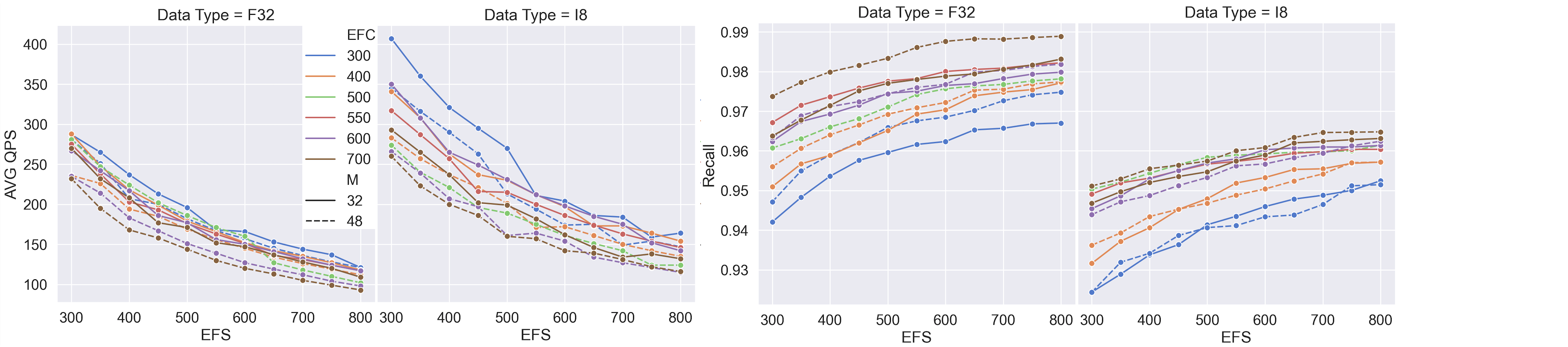
Figure 2. QPS and Recall versus EFS. Quantization results in higher overall QPS at only a slight decrease in recall.

We focus our evaluation on the Hierarchical Navigable Small World (HNSW) algorithm (Malkov and Yashunin, 2018), which has consistently measured as one of the top-performing methods on public benchmarks and remains a popular choice for industry applications. HNSW is a graph traversal algorithm that involves constructing a layered graph from the set of vector embeddings. To measure the scalability of our proposed techniques on a real-world dataset, we focus our evaluation on a collection of 60 million vector representations of products sampled from the catalog of a large e-commerce search engine, using the approach described in (Nigam et al., 2019) to learn the embeddings. We refer to this benchmark as PRODUCT60M. This benchmark also provides 1000 search queries represented by embeddings in the same semantic search space, which we used for recall measurements. In addition, to provide evidence of the generality of our approach, we also consider two additional popular Knn algorithms, namely FAISS  (Johnson et al., 2017) and NGT (Iwasaki and Miyazaki, 2018), and two public benchmark datasets from  Aumüller et al. (2018). In all of our experiments, we fix $k$, the number of nearest neighbors to retrieve, to 100. We analyzed each of these algorithms with and without compressing the embedding vectors and report results relating to (1) memory footprint, (2) indexing time, (3) throughput, and (4) recall. All experiments were run on a single AWS r5n.24xlarge instance with Xeon(R) Platinum CPU 2.50GHz. For measuring indexing time, we used all available CPU cores. For measuring throughput, we used a single thread.

5.2. Experimental Design

We used an open source implementation of HNSW known as HNSWLib. HNSWlib supports only float32 for both indexing and the computation of inner product distance. In order to use int8 for this analysis, we extended the implementation to support both indexing and similarity search on dense embedding vectors represented by int8 arrays. HNSW uses three hyper parameters referred to as EFC, M, and EFS. These parameters have an effect on memory, build time, recall, and throughput. The EFC parameter sets the number of closest elements to the query that are stored within each layer of the HNSW graph during construction time, implying that a higher EFC leads to a more accurate search index but at the cost of a longer build time; the M parameter determines the maximum number of outgoing edges in the graph and heavily influences the memory footprint of the search index; finally, the EFS parameter is analogous to EFC except that it controls the number of neighbors dynamically stored at search time. In this study, we considered a range of values for each hyper parameter when we measured performance. We used two M values, 32 and 48, values from 300 to 700 in increments of 100 for EFC, and 300 to 800 in increments of 50 for EFS.

5.3. Evaluation Metrics

We divide our metrics into two distinct categories: search performance and search quality. For performance, we focused on throughput, the number of queries the algorithm can process per unit of time, and index build time. We measure throughput by evaluating a test query, recording its execution time with no other processes running, and then returning the reciprocal value as a measure of queries per second (QPS). Following the standard in the literature, our primary metric for measuring search quality is recall, defined as $\frac{|S_{E}\cap S_{A}|}{|S_{E}|}$ where $S_{E}$ is the set of results returned by an exact Knn search and $S_{A}$ is the items retrieved by our approximation algorithm.

5.4. Build time and Memory

We built two groups of HNSW indexes for each of the hyper parameter combinations reported above. The first group was built using the original floating point embedding vectors. The second group was built by compressing those vectors using the method described in Section 4. Table 1 summarizes our observations on build time and memory footprint for the two groups, and shows a noticeable improvement for the compressed indexes. Specifically, the int8 indices required approximately half the memory and build time of the float32 indices. We note that the transition from float32 to int8 did not produce a linear decrease in memory. This is due to the overhead of HNSW’s indexing graph data structure which consists entirely of native pointers.

5.5. Throughput

Figure 2 plots QPS as a function of the HNSW search parameter, EFS. The results were computed for several parameter settings which have a non-trivial effect on throughput. The int8 indexes produce higher throughput than the float32 indices. This phenomenon is likely due to the reduced overhead of native int8 operations versus native float32 operations. We observed that there is a negative non-linear association between the search parameter EFS and QPS. This is expected, as higher EFS values correspond to longer search times.

5.6. Recall

As noted in Section 3, the primary source of recall loss for distance metrics which obey the triangle inequality is equality relaxation. Figure 2 reports the relationship between HNSW parameters and recall. The original float32 indices achieve a higher overall recall than the compressed int8 indices, but only by around 2%. Furthermore, as the value of the search parameter EFS increases, so too does recall. This observation suggests that our quantization scheme achieves its goal of preserving relative distances for nearest neighbors at the cost of accepting some aliasing errors for points which are further apart. We also see similar small losses in recall when we evaluated on additional algorithms and datasets, as shown in Tables 2 and 3.

5.7. Extended Evaluation

Our primary evaluation used HNSWlib along with the PRODUCT60M dataset due to the observation that HNSW offered the best recall-QPS tradeoff. However, to provide some evidence for the generality of our approach and its expected performance on other domains and algorithms, we consider two other KNN algorithms and public datasets, specifically the FAISS  (Johnson et al., 2017) exact search implementation and Neighborhood Graph and Tree (NGT) (Iwasaki and Miyazaki, 2018).

Dataset	Distance type	Recall@100
		fp32	int8
SIFT	L2	0.999	0.974
Glove100	Angular	1.0	0.943
PRODUCT60M	IP	1.0	0.983

Table 2. (float32) versus compressed (int8) datasets using FAISS exhaustive nearest neighbor search.

Dataset	Distance type	Recall@100
		fp32	int8
SIFT	L2	0.999	0.974
Glove100	Angular	0.991	0.943
PRODUCT60M	IP	0.972	0.949

Table 3. (float32) versus compressed (int8) data sets using Neighborhood Graph and Tree (NGT).

In addition to the search dataset described in Section 4 we used two public data sets from the KNN benchmark  (Aumüller et al., 2018). The SIFT and Glove100 datasets have dimensions of 128 and 100 respectively, and consist of approximately 1 million vectors each. Each data set has its own 1000 vector test set along with 100 true neighbors for each test vector. Table 2 reports the performance of FAISS both before and after quantization. Table  3 reports the same for NGT. In both cases we were able to achieve comparable improvements in runtime and memory consumption at a slightly larger, though still modest, decrease in recall of $2-6\%$.

6. Future Work and Conclusion

We propose a low precision quantization technique based on the observation that most real-world vector datasets are concentrated in a narrow range that does not require full float32 precision. We applied this technique to the HNSW Knn algorithm and obtained a $60\%$ reduction in memory overhead and a $30\%$ increase in throughput at only a $2\%$ reduction in recall. We also provided evidence of the generality of our method by obtaining similar performance improvements on the FAISS exact search and NGT frameworks. For future work, we hope to further demonstrate the generality of our technique by evaluating on additional Knn algorithms and real-world benchmark datasets and extend our evaluation to additional distance metrics.

References

- (1)
- Amato and Falchi (2010) Giuseppe Amato and Fabrizio Falchi. 2010. KNN Based Image Classification Relying on Local Feature Similarity. In Proceedings of the Third International Conference on SImilarity Search and APplications (Istanbul, Turkey) (SISAP ’10). Association for Computing Machinery, New York, NY, USA, 101–108. https://doi.org/10.1145/1862344.1862360
- Andoni et al. (2015) Alexandr Andoni, Piotr Indyk, Thijs Laarhoven, Ilya Razenshteyn, and Ludwig Schmidt. 2015. Practical and optimal LSH for angular distance. In Advances in neural information processing systems. 1225–1233.
- Aumüller et al. (2018) Martin Aumüller, Erik Bernhardsson, and Alexander John Faithfull. 2018. ANN-Benchmarks: A Benchmarking Tool for Approximate Nearest Neighbor Algorithms. CoRR abs/1807.05614 (2018). arXiv:1807.05614 http://arxiv.org/abs/1807.05614
- Aumüller et al. (2020) Martin Aumüller, Erik Bernhardsson, and Alexander John Faithfull. 2020. ANN-Benchmarks: A benchmarking tool for approximate nearest neighbor algorithms. Inf. Syst. 87 (2020). https://doi.org/10.1016/j.is.2019.02.006
- Babenko and Lempitsky (2014) Artem Babenko and Victor Lempitsky. 2014. Additive quantization for extreme vector compression. In Proceedings of the IEEE Conference on Computer Vision and Pattern Recognition. 931–938.
- Bachrach et al. (2014) Yoram Bachrach, Yehuda Finkelstein, Ran Gilad-Bachrach, Liran Katzir, Noam Koenigstein, Nir Nice, and Ulrich Paquet. 2014. Speeding up the xbox recommender system using a euclidean transformation for inner-product spaces. In Proceedings of the 8th ACM Conference on Recommender systems. 257–264.
- Dasgupta and Freund (2008) Sanjoy Dasgupta and Yoav Freund. 2008. Random projection trees and low dimensional manifolds. In Proceedings of the fortieth annual ACM symposium on Theory of computing. 537–546.
- Garcia et al. (2008) Vincent Garcia, Eric Debreuve, and Michel Barlaud. 2008. Fast k nearest neighbor search using GPU. In 2008 IEEE Computer Society Conference on Computer Vision and Pattern Recognition Workshops. IEEE, 1–6.
- Ge et al. (2013) Tiezheng Ge, Kaiming He, Qifa Ke, and Jian Sun. 2013. Optimized product quantization for approximate nearest neighbor search. In Proceedings of the IEEE Conference on Computer Vision and Pattern Recognition. 2946–2953.
- Guo et al. (2020) Ruiqi Guo, Philip Sun, Erik Lindgren, Quan Geng, David Simcha, Felix Chern, and Sanjiv Kumar. 2020. Accelerating large-scale inference with anisotropic vector quantization. In International Conference on Machine Learning. PMLR, 3887–3896.
- Han et al. (2015) Song Han, Huizi Mao, and William J Dally. 2015. Deep compression: Compressing deep neural networks with pruning, trained quantization and huffman coding. arXiv preprint arXiv:1510.00149 (2015).
- Harwood and Drummond (2016) Ben Harwood and Tom Drummond. 2016. Fanng: Fast approximate nearest neighbour graphs. In Proceedings of the IEEE Conference on Computer Vision and Pattern Recognition. 5713–5722.
- He et al. (2013) Kaiming He, Fang Wen, and Jian Sun. 2013. K-means hashing: An affinity-preserving quantization method for learning binary compact codes. In Proceedings of the IEEE conference on computer vision and pattern recognition. 2938–2945.
- Huang et al. (2013) Po-Sen Huang, Xiaodong He, Jianfeng Gao, Li Deng, Alex Acero, and Larry Heck. 2013. Learning Deep Structured Semantic Models for Web Search using Clickthrough Data. ACM International Conference on Information and Knowledge Management (CIKM). https://www.microsoft.com/en-us/research/publication/learning-deep-structured-semantic-models-for-web-search-using-clickthrough-data/
- Iwasaki and Miyazaki (2018) Masajiro Iwasaki and Daisuke Miyazaki. 2018. Optimization of Indexing Based on k-Nearest Neighbor Graph for Proximity Search in High-dimensional Data. CoRR abs/1810.07355 (2018). arXiv:1810.07355 http://arxiv.org/abs/1810.07355
- Jegou et al. (2010) Herve Jegou, Matthijs Douze, and Cordelia Schmid. 2010. Product quantization for nearest neighbor search. IEEE transactions on pattern analysis and machine intelligence 33, 1 (2010), 117–128.
- Johnson et al. (2017) Jeff Johnson, Matthijs Douze, and Hervé Jégou. 2017. Billion-scale similarity search with GPUs. arXiv preprint arXiv:1702.08734 (2017).
- Johnson et al. (2019) Jeff Johnson, Matthijs Douze, and Hervé Jégou. 2019. Billion-scale similarity search with GPUs. IEEE Transactions on Big Data (2019).
- Kim et al. (2017) J. Kim, C. Park, J. Ahn, Y. Ko, J. Park, and J. C. Gallagher. 2017. Real-time UAV sound detection and analysis system. In 2017 IEEE Sensors Applications Symposium (SAS). 1–5.
- Li et al. (2017) Hui Li, Tsz Nam Chan, Man Lung Yiu, and Nikos Mamoulis. 2017. FEXIPRO: fast and exact inner product retrieval in recommender systems. In Proceedings of the 2017 ACM International Conference on Management of Data. 835–850.
- Malkov and Yashunin (2018) Yury A Malkov and Dmitry A Yashunin. 2018. Efficient and robust approximate nearest neighbor search using hierarchical navigable small world graphs. IEEE transactions on pattern analysis and machine intelligence (2018).
- Martinez et al. (2014) Julieta Martinez, Holger H Hoos, and James J Little. 2014. Stacked quantizers for compositional vector compression. arXiv preprint arXiv:1411.2173 (2014).
- Muja and Lowe (2014) Marius Muja and David G Lowe. 2014. Scalable nearest neighbor algorithms for high dimensional data. IEEE transactions on pattern analysis and machine intelligence 36, 11 (2014), 2227–2240.
- Nigam et al. (2019) Priyanka Nigam, Yiwei Song, Vijai Mohan, Vihan Lakshman, Weitian Ding, Ankit Shingavi, Choon Hui Teo, Hao Gu, and Bing Yin. 2019. Semantic product search. In Proceedings of the 25th ACM SIGKDD International Conference on Knowledge Discovery & Data Mining. 2876–2885.
- Norouzi and Fleet (2013) Mohammad Norouzi and David J Fleet. 2013. Cartesian k-means. In Proceedings of the IEEE Conference on computer Vision and Pattern Recognition. 3017–3024.
- Shrivastava and Li (2014) Anshumali Shrivastava and Ping Li. 2014. Asymmetric LSH (ALSH) for sublinear time maximum inner product search (MIPS). In Advances in Neural Information Processing Systems. 2321–2329.
- Suchal and Návrat (2010) Ján Suchal and Pavol Návrat. 2010. Full Text Search Engine as Scalable k-Nearest Neighbor Recommendation System. In Artificial Intelligence in Theory and Practice III, Max Bramer (Ed.). Springer Berlin Heidelberg, Berlin, Heidelberg, 165–173.
- Teflioudi and Gemulla (2016) Christina Teflioudi and Rainer Gemulla. 2016. Exact and approximate maximum inner product search with lemp. ACM Transactions on Database Systems (TODS) 42, 1 (2016), 1–49.
- Wang et al. (2013) B. Wang, Q. Liao, and C. Zhang. 2013. Weight Based KNN Recommender System. In 2013 5th International Conference on Intelligent Human-Machine Systems and Cybernetics, Vol. 2. 449–452.
- Zhang et al. (2014) Ting Zhang, Chao Du, and Jingdong Wang. 2014. Composite Quantization for Approximate Nearest Neighbor Search.. In ICML, Vol. 2. 3.
- Zhang et al. (2015) Ting Zhang, Guo-Jun Qi, Jinhui Tang, and Jingdong Wang. 2015. Sparse composite quantization. In Proceedings of the IEEE Conference on Computer Vision and Pattern Recognition. 4548–4556.