Variance Reduction based Experience Replay for Policy Optimization

Abstract

For reinforcement learning on complex stochastic systems where many factors dynamically impact the output trajectories, it is desirable to effectively leverage the information from historical samples collected in previous iterations to accelerate policy optimization. Classical experience replay allows agents to remember by reusing historical observations. However, the uniform reuse strategy that treats all observations equally overlooks the relative importance of different samples. To overcome this limitation, we propose a general variance reduction based experience replay (VRER) framework that can selectively reuse the most relevant samples to improve policy gradient estimation. This selective mechanism can adaptively put more weight on past samples that are more likely to be generated by the current target distribution. Our theoretical and empirical studies show that the proposed VRER can accelerate the learning of optimal policy and enhance the performance of state-of-the-art policy optimization approaches.

Keywords Reinforcement Learning  $\cdot$ Policy Optimization  $\cdot$ Multiple Important Sampling  $\cdot$ Variance Reduction  $\cdot$ Experience Replay  $\cdot$ Markov Decision Process

1 Introduction

In recent years, various policy optimization approaches are developed to solve challenging control problems in healthcare (Yu et al., 2021; Zheng et al., 2021), continuous control tasks (Lillicrap et al., 2016; Schulman et al., 2015a, 2017), and biomanufacturing (Zheng et al., 2022). These approaches often consider parametric policies and search for optimal solution through policy gradient approach (Sutton and Barto, 2018), whose performance and convergence crucially depends on the accuracy of gradient estimation. Reusing historical observations is one way to improve gradient estimation, especially when historical data is scarce. In this paper, we address an important question in policy optimization methods: How to intelligently select and reuse historical samples to accelerate the learning of the optimal policy for complex stochastic systems?

According to the different basic unit of historical samples to reuse, policy gradient (PG) algorithms can be classified into episode-based and step-based approaches (Metelli et al., 2020). Episode-based approaches can reuse historical trajectories through importance sampling (IS) strategy accounting for the distributional difference induced by the target and behavioral policies. In this case, the importance sampling weight is built on the product of likelihood ratios (LR) of state-action transitions occurring within each process trajectory. As a result, the likelihood-ratio-weighted observations can have large or even infinite variance, especially for problems with long planning horizons (Schlegel et al., 2019). On the other hand, the step-based approaches take individual state-action transitions as the basic reuse units. This overcomes the limitation of episode-based approaches, provide a more flexible reuse strategy, and support process online control. In this paper, we will develop a general experience replay framework applicable to both episode- and step-based approaches.

For complex stochastic systems such as healthcare (Hall et al., 2012) and biopharmaceutical manufacturing (Zheng et al., 2022), each real or simulation experiment can be financially or computationally expensive. Therefore, it is important to fully utilize all available information when we solve reinforcement learning (RL) optimization problems to guide real-time decision making. On-policy methods only utilize newly generated samples to estimate the policy gradient for each policy update. Ignoring the relevant information carried with historical samples can lead to high uncertainty in policy gradient estimation. Fortunately, this information loss can be reduced through a combination of experience replay (ER) (Lin, 1992; Mnih et al., 2015; Wang et al., 2017) and off-policy optimization methods, which can store and “replay" past relevant experiences to accelerate the search for optimal policy. It often uses importance sampling (IS) mechanism to account for the likelihood mismatch induced by each target policy that we want to assess and the behavioral policy under which past samples were collected (Hesterberg, 1988).

Motivated by the multiple importance sampling (MIS) study presented in Dong et al. (2018), we create a mixture likelihood ratio metamodel that can improve the policy gradient estimation through reusing historical samples. It can compensate the mismatch between target and behavioral distributions so that each historical sample can be used to provide a unbiased prediction of the mean response across the input policy space. However, the reuse of historical samples from behavioral or proposal distributions that are far from the target distribution can lead to the inflated variance on policy gradient estimation.

To avoid this issue, we propose a general variance reduction based experience replay (VRER) framework that can selectively reuse historical samples to reduce the estimation variance of policy gradient and speed up the search for optimal policy. As policy optimization proceeds, this approach can automatically select and reuse the most relevant historical samples generated under visited behavioral policies. The computations required in the proposed selection procedure increase with the number of iterations and the size of historical samples. To circumvent this challenge, we further introduce an approximate selection strategy that dramatically reduces the computational cost. As such, our proposal is computationally efficient and it can support real-time decision making for complex stochastic systems.

Here, we summarize the key contributions and benefits of the proposed framework.

• We propose a general VRER framework for policy gradient optimization. It can accelerate the learning of optimal policy for both step-based and episode-based policy optimization algorithms. This framework is mainly inspired by mixture likelihood ratio (MLR), stochastic gradient variance reduction, and experience replay

• Since each experiment can be very expensive for complex stochastic systems, the proposed VRER can intelligently select and reuse the most relevant historical samples to improve sample efficiency and estimation accuracy of policy gradient.

• Practically, the proposed VRER can be easily applied to most policy gradient optimization methods without structural change. It mainly requires adding the proposed selection procedure before the training step.

• Comprehensive theoretical and empirical studies demonstrate that the proposed VRER framework can efficiently utilize past samples and accelerate the learning of optimal policy for complex stochastic systems.

The organization of this paper is as follows. We review the most related literature studies in Section 2, and present the problem description of general policy gradient optimization for both finite and infinite horizon Markov decision processes (MDPs) in Section 3. We propose the (multiple) importance sampling based policy gradient estimators for both step- and episode-based algorithms in Section 4. Then, we develop the computationally efficient selection rules and propose generic VRER based policy gradient optimization in Section 5. At the end of Section 5, we also provide a finite-time convergence analysis of VRER based policy optimization and show the asymptotic properties. We conclude this paper with the comprehensive empirical study on the proposed framework in Section 6. The implementation of VRER can be found at https://github.com/zhenghuazx/vrer_policy_gradient.

2 Literature Review

The goal of RL is to learn the optimal policy through dynamic interactions with the systems of interest to achieve the best reward (Sutton and Barto, 2018). Stochastic gradient descent or ascent approaches are often used to solve RL problems (Sutton et al., 1999a). The study of policy optimization can be traced back to REINFORCE, also known as vanilla policy gradient (VPG) (Williams, 1992). Later on, Konda and Tsitsiklis (1999); Sutton et al. (1999b) introduced a functional approximation of value function to policy gradient optimization, which is also referred as actor-critic method. Many approaches have been proposed to improve its performance in terms of better sample efficiency, scalability, and rate of convergence in the recent years. For example, Soft Actor-Critic (SAC) incorporates the entropy measure of policy into the reward objective to encourage exploration (Haarnoja et al., 2018). To improve training or prediction reliability, the trust region policy optimization (TRPO) enforces a KL divergence constraint on the size of policy update at each iteration to avoid too much policy parameter change in one update (Schulman et al., 2015a).

For both on-policy and off-policy RL, effective policy optimization algorithms should account for the variance of policy gradient estimation (Metelli et al., 2020). An early attempt from Williams (1992) subtracts a baseline (some value does not depend on the action) from the gradient estimator to reduce its variance without introducing bias. Recent modern policy optimization methods typically use the value function as baseline to reduce the variance of the critic estimator; see for example (Bhatnagar et al., 2009).

Important sampling (IS) has been widely applied to improve policy optimization. Traditionally, it was often used for off-policy value evaluation and policy correction through likelihood ratio between the target policy and the behavior policy (Jiang and Li, 2016; Precup, 2000; Degris et al., 2012). However, IS estimators can suffer from large variance, which motivates the development of variance reduction techniques (Mahmood and Sutton, 2015; Wu et al., 2018; Lyu et al., 2020). For example, Espeholt et al. (2018) presents an IS weighted actor-critic architecture that adopts “retrace" (Munos et al., 2016), a method truncating IS weight with a upper bound to resolve the high variance issue. Metelli et al. (2020) propose the Policy Optimization via Importance Sampling (POIS) approach which optimizes a surrogate objective function accounting for the trade–off between the estimated performance improvement and variance inflation induced by IS. IS is also studied in the simulation literature; for example Feng and Staum (2017); Dong et al. (2018) propose green simulation approach that reuses outputs from past experiments to create an metamodel predicting system mean response and support experiment design.

Experience replay and its extension, such as prioritized experience replay (Schaul et al., 2016), are often used in the policy gradient and RL algorithms to reduce data correlation and improve sample efficiency. Wang et al. (2017) propose actor-critic with experience replay (ACER) that applies experience replay method to an off-policy actor-critic algorithm. This study uses the IS weight to account for the discrepancy between the proposal and target policy distributions and truncates the importance weight to avoid inflated variance.

An important perspective of policy gradient methods is to prevent dramatic updates in policy parametric space. Driven by this principle, trust region policy optimization (TRPO) (Schulman et al., 2015a) considers a surrogate objective function subject to the trust region constraint which enforces the distance between old and new candidate policies measured by KL-divergence to be small enough. Following the similar idea, proximal policy optimization (PPO) (Schulman et al., 2017) truncates the importance weights to discourage the excessively large policy update. As Metelli et al. (2020) pointed out, although TRPO and PPO represent the state–of–the–art policy optimization approaches in RL that successfully control the updates in the policy parameter space, they fail to account for the uncertainty induced by the IS procedure. Unlike these existing approaches, our proposed reuse selection rule can address both issues via comparing the difference between policy gradient estimation variance between new (target) and old (behavioral) policies. First, the variance based selection rule can avoid large variance induced by reusing out-dated samples. Second, such selection also controls the parameter update with a constraint on the distance between old and new policies, because the large mismatch between two policies leads to large likelihood ratio, which in turn causes large gradient estimation variance.

3 Problem Description

In this section, we first review both finite- and infinite-horizon Markov decision process (MDPs) in Section 3.1. Each experiment on complex stochastic systems can be computationally burdensome and financially expensive. Thus, given a tight budget, it is important to leverage on all relevant information from current and historical experimental samples to accelerate the optimization search, especially for systems with high uncertainty. The proposed variance reduction based experience replay is applicable to general policy gradient approaches as reviewed in Section 3.2. Then, we summarize the regularity assumptions and conditions for policy gradient optimizations to support the asymptotic study of the proposed framework in Section 3.3.

3.1 Markov Decision Process

We formulate the RL problems of interest as a MDP specified by $(\mathcal{S},\mathcal{A},H,r,\mathbb{P},\boldsymbol{s}_{1})$, where $\mathcal{S}$, $\mathcal{A}$, and $H$ are the state space, the action space, and the planning horizon, respectively. For the infinite-horizon problems, we let $H=\infty$, and $H$ is a constant otherwise. At each time $t\in[H]$, the agent observes the state $\boldsymbol{s}_{t}\in\mathcal{S}$, takes an action $\boldsymbol{a}_{t}\in\mathcal{A}$, and receives a reward $r_{t}(\boldsymbol{s}_{t},\boldsymbol{a}_{t})\in\mathbb{R}$. Here $[\cdot]$ represents the sequence of integers from $1$ to $H$. In this study, we consider stochastic policy $\pi_{\boldsymbol{\theta}}:\mathcal{S}\mapsto\mathcal{A}$, defined as a mapping from state space to the action and parameterized by $\boldsymbol{\theta}\in\mathbb{R}^{d}$, i.e., $\boldsymbol{a}_{t}\sim\pi_{\boldsymbol{\theta}}(\boldsymbol{a}|\boldsymbol{s}_{t})$. The probability model $\mathbb{P}$ of the stochastic decision process (SDP) of interest is specified by the state transition probabilities $p(\boldsymbol{s}_{t+1}|\boldsymbol{s}_{t},\boldsymbol{a}_{t})$ for all $t$, as well as the probability $p(\boldsymbol{s}_{1})$ for the initial state, i.e., $\boldsymbol{s}_{1}\sim p(\boldsymbol{s}_{1})$.

At any time $t$, the agent observes the state $\boldsymbol{s}_{t}\in\mathcal{S}$, takes an action $\boldsymbol{a}_{t}\in\mathcal{A}$ by following a parametric policy distribution, $\pi(\boldsymbol{a}_{t}|\boldsymbol{s}_{t};\boldsymbol{\theta})$, and receives a reward $r_{t}(\boldsymbol{s}_{t},\boldsymbol{a}_{t})\in\mathbb{R}$. The performance of the candidate policy is evaluated in terms of the expected return, i.e., the expected discounted sum of the rewards collected along the trajectory $R(\boldsymbol{\tau})\equiv\sum^{H+1}_{t=1}\gamma^{t}r(\boldsymbol{s}_{t},\boldsymbol{a}_{t})$, where $\gamma\in(0,1)$ denotes the discount factor. Let $R_{t}^{\gamma}(H)=\sum^{H+1}_{t^{\prime}=t}\gamma^{t^{\prime}-t}r(\boldsymbol{s}_{t^{\prime}},\boldsymbol{a}_{t^{\prime}})$ denote the total discounted reward from time-step $t$ onwards.

(1) Finite Horizon MDPs. In this case, we can have a finite-length process trajectory, denoted by $\boldsymbol{\tau}\equiv(\boldsymbol{s}_{1},\boldsymbol{a}_{1},\boldsymbol{s}_{2},\boldsymbol{a}_{2},\ldots,\boldsymbol{s}_{H},\boldsymbol{a}_{H},\boldsymbol{s}_{H+1})$, with probability density function

$$D\left(\boldsymbol{\tau};\boldsymbol{\theta}\right)\equiv p(\boldsymbol{s}_{1})\prod^{H}_{t=1}\pi_{\boldsymbol{\theta}}(\boldsymbol{a}_{t}|\boldsymbol{s}_{t})p(\boldsymbol{s}_{t+1}|\boldsymbol{s}_{t},\boldsymbol{a}_{t}).$$ (1)

For the policy $\pi_{\boldsymbol{\theta}}$ specified by $\boldsymbol{\theta}$, we have the state-value and action-value functions

$$V^{\pi_{\boldsymbol{\theta}}}(\boldsymbol{s}_{t})={\mathbb{E}}\left[\left.R^{\gamma}_{t}(H)\right|\boldsymbol{s}_{t};{\pi_{\boldsymbol{\theta}}}\right]~{}~{}\text{ and }~{}~{}Q^{\pi_{\boldsymbol{\theta}}}(\boldsymbol{s}_{t},\boldsymbol{a}_{t})={\mathbb{E}}\left[\left.R^{\gamma}_{t}(H)\right|\boldsymbol{s}_{t},\boldsymbol{a}_{t};{\pi_{\boldsymbol{\theta}}}\right]$$

of the expected total discounted reward-to-go. Our goal is to find the optimal policy, denoted by $\pi_{\boldsymbol{\theta}^{*}}$, that maximizes the expected return,

$$\boldsymbol{\theta}^{\star}=\operatorname*{argmax}_{\boldsymbol{\theta}\in\Theta}\mu(\boldsymbol{\theta})={\mathbb{E}}_{\boldsymbol{\tau}}\left[\left.R(\boldsymbol{\tau})\right|\boldsymbol{\theta}\right]$$ (2)

where $\Theta$ represents the policy parameter space.

(2) Infinite Horizon MDPs. For infinite horizon case, we can further write the objective for the infinite-horizon discounted MDP as

$$\max_{\boldsymbol{\theta}\in\Theta}~{}\mu(\boldsymbol{\theta}) ={\mathbb{E}}\left[\left.\sum_{t=1}^{\infty}\gamma^{t-1}r(\boldsymbol{s}_{t},\boldsymbol{a}_{t})\right|\pi_{\boldsymbol{\theta}}\right]$$

$$=\int d^{\pi_{\boldsymbol{\theta}}}(\boldsymbol{s})\int\pi_{\boldsymbol{\theta}}(\boldsymbol{a}|\boldsymbol{s})r(\boldsymbol{s},\boldsymbol{a})d\boldsymbol{s}d\boldsymbol{a}$$

$$={\mathbb{E}}_{\boldsymbol{s}\sim d^{\pi_{\boldsymbol{\theta}}}(\boldsymbol{s}),\boldsymbol{a}\sim\pi_{\boldsymbol{\theta}}(\boldsymbol{a}|\boldsymbol{s})}[r(\boldsymbol{s},\boldsymbol{a})],$$ (3)

where $d^{{\pi_{\boldsymbol{\theta}}}}(\boldsymbol{s})$ is the discounted state distribution induced by the policy ${\pi_{\boldsymbol{\theta}}}$, defined as

$$d^{\pi_{\boldsymbol{\theta}}}(\boldsymbol{s})=(1-\gamma)\int_{\mathcal{S}}\sum_{t=1}^{\infty}\gamma^{t-1}p(\boldsymbol{s}_{1})p(\boldsymbol{s}_{t}=\boldsymbol{s}|\boldsymbol{s}_{1};{\pi_{\boldsymbol{\theta}}})d\boldsymbol{s}_{1}.$$

We denote the state–occupancy measure of state-action pair by $d^{\pi_{\boldsymbol{\theta}}}(\boldsymbol{s},\boldsymbol{a})=\pi_{\boldsymbol{\theta}}(\boldsymbol{a}|\boldsymbol{s})d^{\pi_{\boldsymbol{\theta}}}(\boldsymbol{s})$. Similarly, we define the state-value and action-value functions

$$V^{\pi_{\boldsymbol{\theta}}}(\boldsymbol{s}) =\lim_{H\rightarrow\infty}{\mathbb{E}}\left[\left.R^{\gamma}_{1}(H)\right|\boldsymbol{s}_{1}=\boldsymbol{s};{\pi_{\boldsymbol{\theta}}}\right]={\mathbb{E}}\left[\left.\sum_{t=1}^{\infty}\gamma^{t-1}r(\boldsymbol{s}_{t},\boldsymbol{a}_{t})\right|\boldsymbol{s}_{1}=\boldsymbol{s};{\pi_{\boldsymbol{\theta}}}\right]$$

$$Q^{\pi_{\boldsymbol{\theta}}}(\boldsymbol{s},\boldsymbol{a}) =\lim_{H\rightarrow\infty}{\mathbb{E}}\left[\left.R^{\gamma}_{1}(H)\right|\boldsymbol{s}_{1}=\boldsymbol{s},\boldsymbol{a}_{1}=\boldsymbol{a};{\pi_{\boldsymbol{\theta}}}\right]={\mathbb{E}}\left[\left.\sum_{t=1}^{\infty}\gamma^{t-1}r(\boldsymbol{s}_{t},\boldsymbol{a}_{t})\right|\boldsymbol{s}_{1}=\boldsymbol{s},\boldsymbol{a}_{1}=\boldsymbol{a};\pi_{\boldsymbol{\theta}}\right].$$

3.2 Generic Policy Gradient

Stochastic policy gradient ascent is a popular method to solve the RL optimization problem (2). At each $k$-th iteration, we can iteratively update the policy parameters by

$$\boldsymbol{\theta}_{k+1}\leftarrow\boldsymbol{\theta}_{k}+\eta_{k}\widehat{\nabla\mu}(\boldsymbol{\theta}_{k}),$$ (4)

where $\eta_{k}$ is learning rate or step size and $\widehat{\nabla\mu}(\boldsymbol{\theta}_{k})$ is an estimator of policy gradient $\nabla\mu(\boldsymbol{\theta}_{k})$. For convenience, $\nabla$ denotes the gradient with respect to $\boldsymbol{\theta}$ unless specified otherwise.

To unify both infinite- and finite-horizon MDPs, we define the basic unit of samples for reuse as a trajectory $\boldsymbol{x}=\boldsymbol{\tau}$ for finite horizon MDP or a state-action pair $\boldsymbol{x}=(\boldsymbol{s},\boldsymbol{a})$ for infinite horizon MDP. We let the sampling distribution of each trajectory observation $\rho_{\boldsymbol{\theta}}(\boldsymbol{x})=D(\boldsymbol{\tau};\boldsymbol{\theta})$ for finite-horizon case and each state-action transition observation $\rho_{\boldsymbol{\theta}}(\boldsymbol{x})=d^{\pi_{\boldsymbol{\theta}}}(\boldsymbol{s},\boldsymbol{a})$ for infinite-horizon case. The unified notations will allow us to develop a generic VRER framework for both step- and episode-based algorithms in the following sections.

Under some regular conditions (Sutton et al., 1999b; Baxter and Bartlett, 2001; Williams, 1992), the generic policy gradient is shown as

$$\nabla\mu(\boldsymbol{\theta})\equiv{\mathbb{E}}_{\boldsymbol{x}\sim\rho_{\boldsymbol{\theta}}(\boldsymbol{x}|\boldsymbol{\theta})}[g(\boldsymbol{x})|\boldsymbol{\theta}]=\begin{cases}{\mathbb{E}}_{\boldsymbol{\tau}\sim D(\boldsymbol{\tau};\boldsymbol{\theta})}\left[R(\boldsymbol{\tau})\sum^{H}_{t=1}\nabla\log\pi_{\boldsymbol{\theta}}(\boldsymbol{a}_{t}|\boldsymbol{s}_{t})\right],&\text{finite horizon}\\ {\mathbb{E}}_{(\boldsymbol{s},\boldsymbol{a})\sim d^{\pi_{\boldsymbol{\theta}}}}\left[A^{\pi_{\boldsymbol{\theta}}}(\boldsymbol{s},\boldsymbol{a})\nabla\log\pi_{\boldsymbol{\theta}}(\boldsymbol{a}|\boldsymbol{s})\right],&\text{infinite horizon}\end{cases}$$ (5)

where $A^{\pi_{\boldsymbol{\theta}}}(\boldsymbol{s},\boldsymbol{a})\equiv Q^{\pi_{\boldsymbol{\theta}}}(\boldsymbol{s},\boldsymbol{a})-V^{\pi_{\boldsymbol{\theta}}}(\boldsymbol{s})$ is called advantage and it intuitively measures the extra reward that an agent can obtain by taking a particular action $\boldsymbol{a}$. This leads to the scenario-based policy gradient estimate,

$$g_{k}\left(\boldsymbol{x}\right)\equiv g\left(\boldsymbol{x}|\boldsymbol{\theta}_{k}\right)=\begin{cases}R(\boldsymbol{\tau})\sum^{H}_{t=1}\nabla\log\pi_{\boldsymbol{\theta}}(\boldsymbol{a}_{t}|\boldsymbol{s}_{t}),&\text{finite horizon}\\ A^{\pi_{\boldsymbol{\theta}}}(\boldsymbol{s},\boldsymbol{a})\nabla\log\pi_{\boldsymbol{\theta}}(\boldsymbol{a}|\boldsymbol{s}),&\text{infinite horizon}.\end{cases}$$ (6)

The baseline classical policy gradient (PG) estimator in the $k$-th iteration is given by

$$\widehat{\nabla\mu}^{PG}_{k}\equiv\widehat{\nabla\mu}^{PG}(\boldsymbol{\theta}_{k})=\frac{1}{n}\sum_{j=1}^{n}g_{k}\left(\boldsymbol{x}^{(k,j)}\right).$$ (7)

This is estimated by using $n$ new generated samples in the $k$-th iteration. It can be challenging to precisely estimate the policy gradient $\nabla\mu(\boldsymbol{\theta})$ in (5), especially when process stochasticity is high and each experiment is expensive. The on-policy policy optimization algorithms only use new samples generated in the $k$-th iteration; while all historical observations are discarded. As the samples from previous iterations often have relevant information for estimating the policy gradient in the current iteration, inspired by the importance sampling design paradigm (Feng and Staum, 2017; Metelli et al., 2020), we propose reusing historical samples to improve the estimation accuracy on policy gradient with the likelihood ratio accounting for the difference between the proposal and target distributions.

3.3 Regularity Conditions for Generic Policy Gradient Estimation

We summarize the standard assumptions and conditions for the regularity of generic policy gradient and MDPs, which will be used throughout this paper.

1. (Bounded variance) There exists a constant $\sigma>0$ that bounds the mean square error of classical PG estimator, i.e., ${\mathbb{E}}[\|\widehat{\nabla\mu}^{PG}(\boldsymbol{\theta})-\nabla\mu(\boldsymbol{\theta})\|^{2}]^{1/2}\leq\sigma$ for any $\boldsymbol{\theta}\in\mathbb{R}^{d}$.

2. Suppose the reward function and the policy $\pi_{\boldsymbol{\theta}}$ satisfy the following conditions:

   1. The absolute value of the reward $r(\boldsymbol{s},\boldsymbol{a})$ is bounded uniformly, i.e., there exists a constant, say $U_{r}>0$ such that $|r(\boldsymbol{s},\boldsymbol{a})|\leq U_{r}$ for any $(\boldsymbol{s},\boldsymbol{a})\in\mathcal{S}\times\mathcal{A}$.

   2. The policy $\pi_{\boldsymbol{\theta}}$ is differentiable with respect to $\boldsymbol{\theta}$, and the score function is Lipschitz continuous and has bounded norm, i.e., for any $(\boldsymbol{s},\boldsymbol{a})\in\mathcal{S}\times\mathcal{A}$, there exist positive constant bounds, denoted by $L_{\Theta},U_{\Theta}$, and $U_{\pi}$, such that

      $$\|\nabla\log\pi_{\boldsymbol{\theta}_{1}}(\boldsymbol{a}|\boldsymbol{s})-\nabla\log\pi_{\boldsymbol{\theta}_{2}}(\boldsymbol{a}|\boldsymbol{s})\|\leq L_{\Theta}\|\boldsymbol{\theta}_{1}-\boldsymbol{\theta}_{2}\|\text{ for any $\boldsymbol{\theta}_{1}$ and $\boldsymbol{\theta}_{2}$};$$ (8)

      $$\|\nabla\log\pi_{\boldsymbol{\theta}}(\boldsymbol{a}|\boldsymbol{s})\|\leq U_{\Theta}\text{ for any $\boldsymbol{\theta}$};$$ (9)

      $$\|\pi_{\boldsymbol{\theta}_{1}}(\cdot|\boldsymbol{s})-\pi_{\boldsymbol{\theta}_{2}}(\cdot|\boldsymbol{s})\|_{TV}\leq U_{\pi}\|\boldsymbol{\theta}_{1}-\boldsymbol{\theta}_{2}\|\text{ for any $\boldsymbol{\theta}_{1}$ and $\boldsymbol{\theta}_{2}$}.$$ (10)

      where $d_{TV}(P,Q)$ is the total variation norm between two probability measure $P$ and $Q$, which is defined as $d_{TV}(P,Q)=1/2\int_{\mathcal{X}}|P(dx)-Q(dx)|$.

3. (Independence) For infinite-horizon MDP, the random tuples $(\boldsymbol{s}_{t},\boldsymbol{a}_{t},\boldsymbol{s}_{t+1})$ with $t=1,2,\ldots,$ are drawn from the stationary distribution of the Markov decision process independently across time (Kumar et al., 2019).

Assumption A.1 is a standard assumption that is often used in stochastic approximation analysis. A.1 was originally introduced by Robbins and Monro (1951) and it is defined based on the bound of the $L_{2}$ norm inducing a metric $d(X,Y)=\|X-Y\|_{2}$. It states that the classical PG estimator, denoted by $\widehat{\nabla\mu}^{PG}(\boldsymbol{\theta})$, is unbiased and has bounded variance. The first two items in A.2 are standard assumptions on the regularity of the MDP problem and the parameterized policy, which are the same conditions used in many recent studies (Wu et al., 2020; Zhang et al., 2020; Kumar et al., 2019). The third item is adopted from Xu et al. (2020) which holds for any smooth policy with bounded action space or Gaussian policy; see Lemma 1 in Xu et al. (2020). The independence assumption A.3 does not hold in practice, but it is a standard used to deal with convergence bounds for infinite-horizon MDP problems (Kumar et al., 2019; Wang et al., 2020; Qiu et al., 2021).

The uniform boundedness of the reward function $r(\boldsymbol{s},\boldsymbol{a})$ in Assumption A.2(i) also implies that the absolute value of the Q-function is upper bounded by $\frac{U_{r}}{1-\gamma}$, since by definition

$$|Q^{\pi_{\boldsymbol{\theta}}}(\boldsymbol{s},\boldsymbol{a})|\leq\sum^{\infty}_{t=1}\gamma^{t-1}U_{r}=\frac{U_{r}}{1-\gamma},\text{ for any $(\boldsymbol{s},\boldsymbol{a})\in\mathcal{S}\times\mathcal{A}$}.$$ (11)

The same bound also applies for $V^{\pi_{\boldsymbol{\theta}}}(\boldsymbol{s})$ for any $\boldsymbol{\theta}$ and $\boldsymbol{s}\in\mathcal{S}$

$$|V^{\pi_{\boldsymbol{\theta}}}(\boldsymbol{s})|\leq|{\mathbb{E}}\left[Q^{\pi_{\boldsymbol{\theta}}}(\boldsymbol{s},\boldsymbol{a})\right]|\leq{\mathbb{E}}\left[|Q^{\pi_{\boldsymbol{\theta}}}(\boldsymbol{s},\boldsymbol{a})|\right]\leq\sum^{\infty}_{t=1}\gamma^{t-1}U_{r}=\frac{U_{r}}{1-\gamma}.$$ (12)

This applies to the objective $\mu(\boldsymbol{\theta})$ because $|\mu(\boldsymbol{\theta})|=|{\mathbb{E}}[V^{\pi_{\boldsymbol{\theta}}}(\boldsymbol{s})]|\leq\frac{U_{r}}{1-\gamma}$. In the similar way, we can show for a finite-horizon MDP, the objective is bounded by $|\mu(\boldsymbol{\theta})|\leq HU_{r}$. Thus, we have the bound of the objective as $U_{\mu}=\frac{U_{r}}{1-\gamma}$ for infinite horizon MDP and $U_{\mu}=HU_{r}$ for finite horizon MDP.

Under Assumption A.2, we can establish the Lipschitz continuity of the policy gradient $\nabla\mu(\boldsymbol{\theta})$ as shown Lemma 1. The proof is deferred to Lemma 3.2 in Zhang et al. (2020). Lemma 1 is another essential condition to ensure the convergence of many gradient decent based algorithms; see for example Niu et al. (2011); Reddi et al. (2016); Nemirovski et al. (2009); Li and Orabona (2019). It implies that the gradient cannot change abruptly, i.e., $|\mu(\boldsymbol{\theta}_{2})-\mu(\boldsymbol{\theta}_{1})-\langle\nabla\mu(\boldsymbol{\theta}_{1}),\boldsymbol{\theta}_{2}-\boldsymbol{\theta}_{1}\rangle|\leq L\lVert\boldsymbol{\theta}_{2}-\boldsymbol{\theta}_{1}\rVert^{2}$ (Nesterov (2003), Lemma 1.2.3).

Lemma 1 (Zhang et al. (2020), Lemma 3.2).

Under Assumption A.2, the policy gradient $\nabla\mu(\boldsymbol{\theta})$ is Lipschitz continuous with some constant $L>0$, i.e., for any $\boldsymbol{\theta}_{1},\boldsymbol{\theta}_{2}\in\mathbb{R}^{d}$,

$$\|\nabla\mu(\boldsymbol{\theta}_{1})-\nabla\mu(\boldsymbol{\theta}_{2})\|\leq L\lVert\boldsymbol{\theta}_{1}-\boldsymbol{\theta}_{2}\rVert.$$

At the end of this section, we present Lemma 2 that establishes the boundedness of policy gradient and its stochastic estimate. There exists a constant $M>0$ such that the $L_{2}$ norm of the scenario-based policy gradient estimate is bounded, i.e., $\|g(\boldsymbol{x})\|\leq M$.

Lemma 2 (Properties of Stochastic Policy Gradients).

For any $\boldsymbol{\theta}$, the norm of the policy gradient $\nabla\mu(\boldsymbol{\theta})$ and its scenario-based stochastic estimate $g(\boldsymbol{x}|\boldsymbol{\theta})$ are bounded, i.e.,

$$g\left(\boldsymbol{x}|\boldsymbol{\theta}\right)\leq M\text{ and }\nabla\mu(\boldsymbol{\theta})\leq M$$

where $M=H^{2}U_{r}U_{\Theta}$ for finite-horizon MDP and $M=\frac{2U_{r}U_{\Theta}}{1-\gamma}$ for infinite-horizon MDP.

Proof.

From Equation (6), we have the scenario-based stochastic gradient estimate

$$\|g\left(\boldsymbol{x}|\boldsymbol{\theta}\right)\| \leq\begin{cases}|\sum^{H}_{t=1}r_{t}|\sum^{H}_{t=1}\|\nabla\log\pi_{\boldsymbol{\theta}}(\boldsymbol{a}_{t}|\boldsymbol{s}_{t})\|,&\text{finite horizon}\\ |Q^{\pi_{\boldsymbol{\theta}}}-V^{\pi_{\boldsymbol{\theta}}}|\|\nabla\log\pi_{\boldsymbol{\theta}}(\boldsymbol{a}|\boldsymbol{s})\|,&\text{infinite horizon}\end{cases}$$

$$\leq\begin{cases}H^{2}U_{r}U_{\Theta},&\text{finite horizon}\\ \frac{2U_{r}U_{\Theta}}{1-\gamma},&\text{infinite horizon}\end{cases}$$ (13)

where step (13) follows Assumption A.2(ii) and the boundness of value functions (Equation (11) and (12)). Let $M=H^{2}U_{r}U_{\Theta}$ for finite-horizon MDP and $M=\frac{2U_{r}U_{\Theta}}{1-\gamma}$ for infinite-horizon MDP. The boundness of policy gradient $\nabla\mu(\boldsymbol{\theta})$ follows the fact that

$$\|\nabla\mu(\boldsymbol{x})\|=\|{\mathbb{E}}_{\rho_{\boldsymbol{\theta}}(\boldsymbol{x})}[g(\boldsymbol{x}|\boldsymbol{\theta})]\|\stackrel{{\scriptstyle(\star)}}{{\leq}}{\mathbb{E}}_{\rho_{\boldsymbol{\theta}}(\boldsymbol{x})}[\|g(\boldsymbol{x}|\boldsymbol{\theta})\|]\stackrel{{\scriptstyle(\star\star)}}{{\leq}}{\mathbb{E}}[M]=M,$$

where step ($\star$) follows by applying Jensen’s inequality and $(\star\star)$ follows by applying (13). ∎

Various policy gradient algorithms are proposed during recent years. The forms of policy gradient estimators may vary from one to another. For example, the total discounted rewards of a trajectory $R(\boldsymbol{\tau})$ can be replaced by the reward-to-go (future total discounted reward after taking action $\boldsymbol{a}_{t}$), i.e., $\sum^{H}_{t^{\prime}=t}\gamma^{t^{\prime}}r_{t^{\prime}}$. The advantage function can be also replaced with action value function or TD residual. Interested readers for other variants are referred to Sutton and Barto (2018) and Schulman et al. (2015b) for the derivations of general policy gradient algorithms. We emphasize that the proposed VRER approach is general and it can be adopted to most policy gradient optimization algorithms. In the empirical study in Section 6, we demonstrate this generality by using three well-known policy optimization algorithms, i.e., VPG, PPO, and TRPO.

4 Mixture Likelihood Ratio Assisted Policy Gradient Estimation

In this section, we describe how to utilize important sampling (IS) and multiple likelihood ratio (MLR) to improve the policy gradient estimation through reusing historical samples. In specific, at each $k$-th iteration, we estimate the performance of the candidate target policy $\pi_{\boldsymbol{\theta}_{k}}$. Let $\rho_{\boldsymbol{\theta}_{k}}(\boldsymbol{x})$ denote the target distribution at the $k$-th iteration and $\rho_{\boldsymbol{\theta}_{i}}(\boldsymbol{x})$ denote the proposal distribution induced by the behavioral policy from the $i$-th iteration. Let $\mathcal{F}_{k}$ denote the set of all behavioral distributions that have been visited by the beginning of the $k$-th iteration. Let $\mathcal{U}_{k}$ be a reuse set with $\mathcal{U}_{k}\subseteq\mathcal{F}_{k}$ including the MDP model candidates whose historical samples are selected and reused for estimating $\nabla\mu(\boldsymbol{\theta}_{k})$. Denote its cardinality as $|\mathcal{U}_{k}|$. For discussions in this section we assume $\mathcal{U}_{k}$ is given. We will present how to design and automatically create the reuse set $\mathcal{U}_{k}$ in Section 5.

4.1 Importance Sampling based Policy Gradient Estimators

Importance sampling is a technique for evaluating the properties of a target distribution $\rho_{\boldsymbol{\theta}_{k}}(\boldsymbol{x})$ of interest by reusing samples generated from a different proposal distribution $\rho_{\boldsymbol{\theta}_{i}}(\boldsymbol{x})$; see Owen (2013). The well-known importance sampling (IS) identity ${\mathbb{E}}_{\boldsymbol{x}\sim\rho_{\boldsymbol{\theta}_{k}}}[g_{k}(\boldsymbol{x})]={\mathbb{E}}_{\boldsymbol{x}\sim\rho_{\boldsymbol{\theta}_{i}}(\boldsymbol{x})}\left[g_{k}(\boldsymbol{x})f_{i,k}(\boldsymbol{x})\right]$ holds provided that $\rho_{\boldsymbol{\theta}_{k}}(\boldsymbol{x})g(\boldsymbol{x})=0$ whenever $\rho_{\boldsymbol{\theta}_{i}}(\boldsymbol{x})=0$, where $f_{i,k}(\boldsymbol{x})={\rho_{\boldsymbol{\theta}_{k}}(\boldsymbol{x})}/{\rho_{\boldsymbol{\theta}_{i}}(\boldsymbol{x})}$ is likelihood ratio (LR). Intuitively, the magnitude of the likelihood ratio is associated with the discrepancy of the probability measures $\rho_{\boldsymbol{\theta}_{k}}$ and $\rho_{\boldsymbol{\theta}_{i}}$. Here we present IS based policy gradient estimators studied in this paper.

(1) Individual Likelihood Ratio (ILR) Policy Gradient Estimator. The policy gradient $\nabla\mu(\boldsymbol{\theta}_{k})$ can be estimated by the individual likelihood estimator (ILR), defined in (14), by using the $n$ historical samples generated by $\rho_{\boldsymbol{\theta}_{i}}(\boldsymbol{x})$,

$$\widehat{\nabla\mu}^{ILR}_{i,k}=\frac{1}{n}\sum^{n}_{j=1}f_{i,k}\left(\boldsymbol{x}^{(i,j)}\right)g_{k}\left(\boldsymbol{x}^{(i,j)}\right)~{}\mbox{with}~{}f_{i,k}(\boldsymbol{x})=\frac{\rho_{\boldsymbol{\theta}_{k}}(\boldsymbol{x})}{\rho_{\boldsymbol{\theta}_{i}}(\boldsymbol{x})}.$$ (14)

The likelihood ratio $f_{i,k}(\boldsymbol{x})$ weights the historical samples appropriately to correct the mismatch between the MDP distributions induced by the behavioral and target policies specified by parameters $\boldsymbol{\theta}_{i}$ and $\boldsymbol{\theta}_{k}$.

One way to reuse all the observations associated with the behavioral distributions included in the reuse set $\mathcal{U}_{k}$ is to average the ILR estimators for all selected proposal distributions, i.e., ${\boldsymbol{\theta}_{i}}\in\mathcal{U}_{k}$, which we call the average ILR policy gradient estimator,

$$\widehat{\nabla\mu}^{ILR}_{k}=\frac{1}{|\mathcal{U}_{k}|}\sum_{{\boldsymbol{\theta}_{i}}\in\mathcal{U}_{k}}\widehat{\nabla\mu}^{ILR}_{i,k}(\boldsymbol{\theta}_{k})=\frac{1}{|\mathcal{U}_{k}|n}\sum_{{\boldsymbol{\theta}_{i}}\in\mathcal{U}_{k}}\sum^{n}_{j=1}\frac{\rho_{\boldsymbol{\theta}_{k}}(\boldsymbol{x}^{(i,j)})}{\rho_{\boldsymbol{\theta}_{i}}(\boldsymbol{x}^{(i,j)})}g_{k}\left(\boldsymbol{x}^{(i,j)}\right).$$ (15)

For simplification, we allocate a constant number of replications (i.e., $n$) for each visit at $\boldsymbol{\theta}$. The estimators in (14) and (15) are unbiased due to the fact

$${\mathbb{E}}_{\rho_{\boldsymbol{\theta}_{i}}}\left[\widehat{\nabla\mu}^{ILR}_{i,k}(\boldsymbol{\theta}_{k})\right]=\int\frac{\rho_{\boldsymbol{\theta}_{k}}(\boldsymbol{x})}{\rho_{\boldsymbol{\theta}_{i}}(\boldsymbol{x})}\rho_{\boldsymbol{\theta}_{i}}(\boldsymbol{x})g_{k}(\boldsymbol{x})\mbox{d}\boldsymbol{x}=\int\rho_{\boldsymbol{\theta}_{k}}\left(\boldsymbol{x}\right)g_{k}\left(\boldsymbol{x}\right)\mbox{d}\boldsymbol{x}=\nabla\mu(\boldsymbol{\theta}_{k}).$$

(2) Mixture Likelihood Ratio (MLR) Policy Gradient Estimator. Though the ILR estimators (14) and (15) are unbiased, their variances could be large or even infinite, as the likelihood ratio $f_{i,k}(\boldsymbol{x})$ can be large or unbounded; see  Veach and Guibas (1995). Thus, the recent studies Feng and Staum (2017); Dong et al. (2018) propose multiple importance sampling or MLR that uses a mixture proposal distribution to overcome this drawback, which can lead to much more stable estimation in different applications.

Instead of viewing the samples from each behavioral proposal distribution $\rho_{\boldsymbol{\theta}_{i}}(\boldsymbol{x})$ in isolation and forming ILR estimators, we can view all the observations associated with $\boldsymbol{\theta}_{i}\in\mathcal{U}_{k}$ collectively as stratified samples from the mixture proposal distribution $\ell_{k}(\boldsymbol{x})=\frac{1}{|\mathcal{U}_{k}|}\sum_{{\boldsymbol{\theta}_{i}}\in\mathcal{U}_{k}}\rho_{\boldsymbol{\theta}_{i}}(\boldsymbol{x})$. This view leads to the mixture likelihood ratio (MLR) policy gradient estimator,

$$\widehat{\nabla\mu}^{MLR}_{k}=\frac{1}{|\mathcal{U}_{k}|n}\sum_{{\boldsymbol{\theta}_{i}}\in\mathcal{U}_{k}}\sum^{n}_{j=1}\left[f_{k}\left(\boldsymbol{x}^{(i,j)}\right)g_{k}\left(\boldsymbol{x}^{(i,j)}\right)\right]~{}\mbox{with}~{}f_{k}(\boldsymbol{x})=\frac{\rho_{\boldsymbol{\theta}_{k}}(\boldsymbol{x})}{\ell_{k}(\boldsymbol{x})}.$$ (16)

The mixture likelihood ratio $f_{k}(\boldsymbol{x})$ reaches its max value when $\rho_{\boldsymbol{\theta}_{i}}(\boldsymbol{x})=0$ for behavioral policies visited in previous iterations. Since we always include the samples generated in the $k$-th iteration, this mixture likelihood ratio is bounded, i.e., $f_{k}(\boldsymbol{x})\leq|\mathcal{U}_{k}|$, which can control the policy gradient estimation variance inflation. In this way, the mixture likelihood ratio puts higher weight on the samples that are more likely to be generated by the target distribution $\rho_{\boldsymbol{\theta}_{k}}$ without assigning extremely large weights on the others.

Lemma 3.

Conditional on $\mathcal{F}_{k}$, the proposed MLR policy gradient estimator is unbiased:

$${\mathbb{E}}\left[\left.\widehat{\nabla\mu}^{MLR}_{k}\right|\mathcal{F}_{k}\right]={\mathbb{E}}\left[\left.g_{k}(\boldsymbol{x})\right|\boldsymbol{\theta}_{k}\right]=\nabla\mu(\boldsymbol{\theta}_{k}).$$

Based on the studies, e.g., Veach and Guibas (1995) and Feng and Staum (2017), we show that the MLR estimator is unbiased in Lemma 3; see the proof in the Appendix (Section B.1). The trace of the covariance matrix $\mbox{Tr}(\mbox{Var}[\widehat{\nabla\mu}(\boldsymbol{\theta})])$ is the total variance of the policy gradient estimator $\widehat{\nabla\mu}(\boldsymbol{\theta})$, which is often considered in many gradient estimation variance reduction studies (Greensmith et al., 2004). This motivates us to use it as the metrics to select historical samples and associated behavioral distributions that can reduce the variance of MLR policy gradient estimators in Section 5. For any $(d\times d)$ matrix $A$, the trace used in the paper is defined as $\mbox{Tr}({A})=\sum_{i=1}^{d}A_{i,i}$. We consider $L_{2}$ norm for any $d$-dimensional vector $\boldsymbol{x}\in\mathbb{R}^{d}$, i.e., $\|\boldsymbol{x}\|\triangleq\|\boldsymbol{x}\|_{2}=\sqrt{\sum_{i=1}^{d}x_{i}^{2}}$. Then, motivated by Martino et al. (2015) Theorem A.2 and Feng and Staum (2017) Proposition 2.5, we can show that conditional on $\mathcal{F}_{k}$, the total variance of the MLR policy gradient estimator is less than that of the average ILR estimator in Proposition 1; see the proof in the Appendix (Section B.2).

Proposition 1.

Conditional on $\mathcal{F}_{k}$, the total variance of the MLR policy gradient estimator (16) is smaller and equal to that of the average ILR policy gradient estimator (15),

$$\mbox{Tr}\left(\mbox{Var}\left[\left.\widehat{\nabla\mu}^{MLR}_{k}\right|\mathcal{F}_{k}\right]\right)\leq\mbox{Tr}\left(\mbox{Var}\left[\left.{\widehat{\nabla\mu}}^{ILR}_{k}\right|\mathcal{F}_{k}\right]\right).$$

(3) Clipped Likelihood Ratio (CLR) Policy Gradient Estimator. Another technique for overcoming the undesirable heavy–tailed behavior is weight clipping (Ionides, 2008). In specific, we can truncate the likelihood ratio $f_{i,k}(\boldsymbol{x})={\rho_{\boldsymbol{\theta}_{k}}(\boldsymbol{x})}/{\rho_{\boldsymbol{\theta}_{i}}(\boldsymbol{x})}$ through applying the operator $\min(f_{i,k}(\boldsymbol{x}),U_{f})$, which sets the max LR to be a pre-specified constant, denoted by $U_{f}$. Formally speaking, the CLR policy gradient estimator can be expressed as

$$\widehat{\nabla\mu}^{CLR}_{k}=\frac{1}{|\mathcal{U}_{k}|}\sum_{{\boldsymbol{\theta}_{i}}\in\mathcal{U}_{k}}\widehat{\nabla\mu}^{CLR}_{i,k}(\boldsymbol{\theta}_{k})=\frac{1}{|\mathcal{U}_{k}|n}\sum_{{\boldsymbol{\theta}_{i}}\in\mathcal{U}_{k}}\sum^{n}_{j=1}\min\left(\frac{\rho_{\boldsymbol{\theta}_{k}}(\boldsymbol{x}^{(i,j)})}{\rho_{\boldsymbol{\theta}_{i}}(\boldsymbol{x}^{(i,j)})},U_{f}\right)g_{k}\left(\boldsymbol{x}^{(i,j)}\right).$$ (17)

Although truncating the likelihood ratios (LRs) introduces a bias, this bias can be bounded as a function of the Rényi divergence and the clipping threshold; see more details in Metelli et al. (2020). Following the similar idea, we derive an upper bound under Assumption A.1, where the bound of bias is expressed as the probability that the LRs are greater than max value $U_{f}$. The proof of Lemma 4 can be found in the Appendix (Section B.4)

Lemma 4.

Suppose that Assumptions A.1, A.2, and A.3 hold. For a clipped likelihood ratio based policy gradient estimator $\widehat{\nabla\mu}^{CLR}_{k}$, with a finite clipping threshold $U_{f}>1$, the bias and the variance of the CLR estimator can be upper bounded as

$$\left\|{\mathbb{E}}\left[\widehat{\nabla\mu}^{CLR}_{k}\right]-\nabla\mu(\boldsymbol{\theta}_{k})\right\|\leq Z(k),$$

$$\mbox{Tr}\left(\mbox{Var}\left[\left.\widehat{\nabla\mu}^{CLR}_{k}\right|\mathcal{F}_{k}\right]\right)\leq\mbox{Tr}\left(\mbox{Var}\left[\left.\widehat{\nabla\mu}^{ILR}_{k}\right|\mathcal{F}_{k}\right]\right)+\frac{1}{n|\mathcal{U}_{k}|}\left\|\nabla\mu(\boldsymbol{\theta}_{k})\right\|^{2},$$

where $Z(k)=\frac{M}{|\mathcal{U}_{k}|}\sum_{{\boldsymbol{\theta}_{i}}\in\mathcal{U}_{k}}{\mathbb{E}}_{k}\left[\mathbbm{1}\left\{{f}_{i,k}(\boldsymbol{x})>U_{f}\right\}\right]$ and $M$ is the bound defined in Lemma 2.

4.2 Policy Gradient Estimation for Finite- and Infinite-Horizon MDPs

(1) Finite-Horizon MDPs. At any $k$-th iteration, importance sampling allows us to compensate the mismatch between the behavioral distribution $\rho_{\boldsymbol{\theta}_{i}}(\boldsymbol{x})$ and the target distribution $\rho_{\boldsymbol{\theta}_{k}}(\boldsymbol{x})$. For policy gradient estimators under finite-horizon MDP, after cancelling the term $p(\boldsymbol{s}_{1})\prod^{H-1}_{t=1}p(\boldsymbol{s}_{t+1}|\boldsymbol{s}_{t},\boldsymbol{a}_{t})$ in the likelihood ratio $f_{i,k}(\boldsymbol{x})={\rho_{\boldsymbol{\theta}_{k}}(\boldsymbol{x})}/{\rho_{\boldsymbol{\theta}_{i}}(\boldsymbol{x})}$, the ILR policy gradient estimators in (15) (similar for CLR estimator (17)) can be simplified to

$$\widehat{\nabla\mu}^{ILR}_{i,k}=\frac{1}{n}\sum^{n}_{j=1}\left[\frac{\prod^{H}_{t=1}\pi_{\boldsymbol{\theta}_{k}}\left(\boldsymbol{a}_{t}^{(i,j)}\left|\boldsymbol{s}_{t}^{(i,j)}\right.\right)}{\prod^{H}_{t=1}\pi_{\boldsymbol{\theta}_{i}}\left(\boldsymbol{a}_{t}^{(i,j)}\left|\boldsymbol{s}_{t}^{(i,j)}\right.\right)}g_{k}\left(\boldsymbol{s}^{(i,j)},\boldsymbol{a}^{(i,j)}\right)\right]\mbox{ and }\widehat{\nabla\mu}^{ILR}_{k}=\frac{1}{|\mathcal{U}_{k}|}\sum_{\boldsymbol{\theta}_{i}\in\mathcal{U}_{k}}\widehat{\nabla\mu}^{ILR}_{i,k},$$

and the MLR policy gradient estimator in (16) can be written as

$$\widehat{\nabla\mu}^{MLR}_{k}=\frac{1}{|\mathcal{U}_{k}|n}\sum_{\boldsymbol{\theta}_{i}\in\mathcal{U}_{k}}\sum^{n}_{j=1}f_{k}\left(\boldsymbol{\tau}^{(i,j)}\right)g_{k}\left(\boldsymbol{\tau}^{(i,j)}\right),~{}\mbox{with}~{}f_{k}\left(\boldsymbol{\tau}\right)=\frac{\prod^{H}_{t=1}\pi_{\boldsymbol{\theta}_{k}}\left(\boldsymbol{a}_{t}\left|\boldsymbol{s}_{t}\right.\right)}{\frac{1}{|\mathcal{U}_{k}|}\sum_{\boldsymbol{\theta}_{i}\in\mathcal{U}_{k}}\prod^{H}_{t=1}\pi_{\boldsymbol{\theta}_{i}}\left(\boldsymbol{a}_{t}\left|\boldsymbol{s}_{t}\right.\right)}.$$

(2) Infinite-Horizon MDPs. For infinite-horizon MDPs, step–based policy gradient algorithms need just a single likelihood ratio per state-action transition sample, i.e.,

$$\nabla\mu(\boldsymbol{\theta}_{k})={\mathbb{E}}_{\rho_{\boldsymbol{\theta}_{i}}}\left[\left.\frac{\rho_{\boldsymbol{\theta}_{k}}(\boldsymbol{s},\boldsymbol{a})}{\rho_{\boldsymbol{\theta}_{i}}(\boldsymbol{s},\boldsymbol{a})}g_{k}(\boldsymbol{x})\right|\boldsymbol{\theta}_{k}\right]={\mathbb{E}}_{\rho_{\boldsymbol{\theta}_{i}}}\left[\left.\frac{\rho_{\boldsymbol{\theta}_{k}}(\boldsymbol{s},\boldsymbol{a})}{\rho_{\boldsymbol{\theta}_{i}}(\boldsymbol{s},\boldsymbol{a})}\nabla\log\pi_{\boldsymbol{\theta}_{k}}(\boldsymbol{a}|\boldsymbol{s})A^{\pi_{\boldsymbol{\theta}_{k}}}(\boldsymbol{s},\boldsymbol{a})\right|\boldsymbol{\theta}_{k}\right].$$ (18)

However, it requires to estimate the stationary distribution $d^{\pi_{\boldsymbol{\theta}}}(\boldsymbol{s})$ in the state–occupancy measure ratios $\rho_{\boldsymbol{\theta}_{k}}(\boldsymbol{s},\boldsymbol{a})=\pi_{\boldsymbol{\theta}_{k}}(\boldsymbol{a}|\boldsymbol{s})d^{\pi_{\boldsymbol{\theta}}}(\boldsymbol{s})$. Unlike finite-horizon MDPs, those ratios cannot be computed in closed form. This problem is also known as distribution corrections (DICE) in RL. Fortunately, a list of approaches has been recently proposed to address this challenge; see Nachum et al. (2019); Yang et al. (2020). The step-based policy gradient estimator (18) can be simplified by introducing bias; for example Degris et al. (2012) proposed an off-policy gradient approximator,

$$\nabla\mu(\boldsymbol{\theta}_{k})\approx{\mathbb{E}}_{\rho_{\boldsymbol{\theta}_{i}}}\left[\left.\frac{\pi_{\boldsymbol{\theta}_{k}}}{\pi_{\boldsymbol{\theta}_{i}}}g_{k}(\boldsymbol{s},\boldsymbol{a})\right|\boldsymbol{\theta}_{k}\right].$$ (19)

It can preserve the set of local optima to which gradient ascent converges. Although biased, this estimator has been widely used in many state-of-the-art off-policy algorithms (Schulman et al., 2015a, 2017; Wang et al., 2017) due to its simplicity and computational efficiency. Following the same idea, the ILR and MLR policy gradient estimators for step-based algorithms can be approximated by replacing $\rho_{\boldsymbol{\theta}}(\boldsymbol{s},\boldsymbol{a})$ with policy $\pi_{\boldsymbol{\theta}}(\boldsymbol{a}|\boldsymbol{s})$. In particular, we could use the approximation $f_{i,k}(\boldsymbol{x})=\frac{\rho_{\boldsymbol{\theta}_{k}}(\boldsymbol{x})}{\rho_{\boldsymbol{\theta}_{i}}(\boldsymbol{x})}\approx\frac{\pi_{\boldsymbol{\theta}_{k}}(\boldsymbol{x})}{\pi_{\boldsymbol{\theta}_{i}}(\boldsymbol{x})}$ in the ILR estimator (14) and the CLR estimator (17), while using $f_{k}(\boldsymbol{x})=\frac{\rho_{\boldsymbol{\theta}_{k}}(\boldsymbol{x})}{\ell_{k}(\boldsymbol{x})}\approx\frac{\pi_{\boldsymbol{\theta}_{k}}(\boldsymbol{a}_{t}|\boldsymbol{s}_{t})}{\sum_{\boldsymbol{\theta}_{i}\in\mathcal{U}_{k}}\pi_{\boldsymbol{\theta}_{k}}(\boldsymbol{a}_{t}|\boldsymbol{s}_{t})}$ in the MLR estimator (16).

We conclude this section by pointing out that we proceed theoretical analysis with the unbiased policy gradient (18) in the following sections. The approximator (19) can be used in the algorithm development and the empirical study to simplify the implementation.

5 Variance Reduction Experience Replay for Policy Optimization

Before one can use the IS based policy gradient estimators developed in Section 4, there is one key remaining question: How to select the behavioral policies, among all historical candidate policies and samples visited up to the $k$-th iteration, to be included in the reuse set $\mathcal{U}_{k}$? Instead of reusing all of them, reusing only the most relevant samples can reduce computational cost, stabilize likelihood ratio calculations, and reduce the gradient estimation variance. In short, a well-designed selection rule can improve sample efficiency and stability of policy gradient estimation and further accelerate the learning of optimal policy.

In Section 5.1, we propose a selection criterion to construct the reuse set $\mathcal{U}_{k}$ so that it can reduce the variance in policy gradient estimation. Since the proposed selection criterion needs to assess all historical samples and associated behavioral policies to determine $\mathcal{U}_{k}$, the likelihood ratio calculations can be computationally expensive as the size of the reuse set increases. Thus, we derive two computationally efficient approximated selection rules in Section 5.2. Based on the proposed selection criteria, we propose the VRER based generic policy gradient optimization algorithm (called PG-VRER) in Section 5.3, and have the convergence analysis in Section 5.4 to show that it can accelerate the policy search. In Section 5.5, we show that the size of the reuse set $|\mathcal{U}_{k}|$ increases to infinity almost surely (a.s.) as the number of iterations increases $k\rightarrow\infty$. The empirical study in Section 6 shows the finite sample performance is consistent with these asymptotic analytical conclusions.

5.1 Reuse Set Selection to Reduce Policy Gradient Estimation Variance

To improve the policy gradient estimation, we want to select the reuse set $\mathcal{U}_{k}$ producing stable likelihood ratios and thus reducing the estimation variance of policy gradient. Even though the target distribution can be high dimensional for complex systems with high uncertainty, the proposed VRER based policy gradient estimators tend to intelligently put more weight on historical observations that are most likely sampled from the target distribution.

Motivated by this insight, we propose a selection criterion in Theorem 1 based on the comparison of variances of the baseline PG estimator (7) and the ILR estimator (14) to dynamically determine the reuse set $\mathcal{U}_{k}$ for each $k$-th iteration. The variance difference between $\widehat{\nabla\mu}^{ILR}_{i,k}$ and $\widehat{\nabla\mu}^{PG}_{k}$ is induced by the discrepancy between the proposal and target distributions, i.e., $\rho_{\boldsymbol{\theta}_{i}}$ and $\rho_{\boldsymbol{\theta}_{k}}$. If $\boldsymbol{\theta}_{i}=\boldsymbol{\theta}_{k}$, the likelihood ratio in (14) equals to 1 so $\widehat{\nabla\mu}^{ILR}_{i,k}=\widehat{\nabla\mu}^{PG}_{k}$, therefore they have the same variance. The proposed selection criterion (20) puts a constant threshold $c$ on the variance inflation of $\widehat{\nabla\mu}^{ILR}_{i,k}$ compared to $\widehat{\nabla\mu}^{PG}_{k}$. It tends to select those behavioral distributions $\rho_{\boldsymbol{\theta}_{i}}(\boldsymbol{x})$ with $\boldsymbol{\theta}_{i}\in\mathcal{F}_{k}$ that are close to the target distribution $\rho_{\boldsymbol{\theta}_{k}}(\boldsymbol{x})$. To ensure that new samples generated in the current $k$-th iteration are always included in the set $\mathcal{U}_{k}$, we consider the constant $c>1$. In addition, Theorem 1 demonstrates that the selection criterion (20) guides an appropriate reuse of historical samples and leads to variance reduction of the ILR and MLR policy gradient estimators compared to the baseline PG estimator by a factor of $c/|\mathcal{U}_{k}|$; see (21). The proof of Theorem 1 can be found in the Appendix (Section B.3).

Theorem 1.

At the $k$-th iteration with the target distribution $\rho_{\boldsymbol{\theta}_{k}}(\boldsymbol{x})$, the reuse set $\mathcal{U}_{k}$ is created to include the behavioral distributions, i.e., $\rho_{\boldsymbol{\theta}_{i}}(\boldsymbol{x})$ with $\boldsymbol{\theta}_{i}\in\mathcal{F}_{k}$, whose the total variance of the ILR policy gradient estimator is no greater than $c$ times that of the classical PG estimator for some constant $c>1$. Mathematically,

$$\text{{Selection Rule 1:}}~{}~{}~{}\mbox{Tr}\left(\mbox{Var}\left[\left.\widehat{\nabla\mu}^{ILR}_{i,k}\right|\mathcal{F}_{k}\right]\right)\leq c\mbox{Tr}\left(\mbox{Var}\left[\left.\widehat{\nabla\mu}^{PG}_{k}\right|\boldsymbol{\theta}_{k}\right]\right)$$ (20)

Then, based on such reuse set $\mathcal{U}_{k}$, the total variance of the MLR/ILR policy gradient estimators (15) and (16) are no greater than $\frac{c}{|\mathcal{U}_{k}|}$ times the total variance of the PG estimator,

$$\mbox{Tr}\left(\mbox{Var}\left[\left.\widehat{\nabla\mu}^{MLR}_{k}\right|\mathcal{F}_{k}\right]\right)\leq\mbox{Tr}\left(\mbox{Var}\left[\left.\widehat{\nabla\mu}^{ILR}_{k}\right|\mathcal{F}_{k}\right]\right)\leq\frac{c}{|\mathcal{U}_{k}|}\mbox{Tr}\left(\mbox{Var}\left[\left.\widehat{\nabla\mu}^{PG}_{k}\right|\boldsymbol{\theta}_{k}\right]\right).$$ (21)

Moreover,

$${\mathbb{E}}\left[\left.\left\|\widehat{\nabla\mu}^{MLR}_{k}\right\|^{2}\right|\mathcal{F}_{k}\right]\leq{\mathbb{E}}\left[\left.\left\|\widehat{\nabla\mu}^{ILR}_{k}\right\|^{2}\right|\mathcal{F}_{k}\right]\leq\frac{c}{|\mathcal{U}_{k}|}{\mathbb{E}}\left[\left.\left\|\widehat{\nabla\mu}^{PG}_{k}\right\|^{2}\right|\boldsymbol{\theta}_{k}\right]+\left(1-\frac{c}{|\mathcal{U}_{k}|}\right)\left\|\nabla\mu(\boldsymbol{\theta}_{k})\right\|^{2}.$$ (22)

With the selection rule (20), Lemma 4 allows us to construct a similar bound on the expected squared norm of CLR policy gradient estimator as the bound (22); see Corollary 1. The proof is provided in the Appendix (Section B.5).

Corollary 1.

At the $k$-th iteration with the target distribution $\rho_{\boldsymbol{\theta}_{k}}(\boldsymbol{x})$, we apply the selection rule from Theorem 1. Then, based on such reuse set $\mathcal{U}_{k}$, we have the following bound

$${\mathbb{E}}\left[\left.\left\|\widehat{\nabla\mu}^{CLR}_{k}\right\|^{2}\right|\mathcal{F}_{k}\right]\leq\frac{c}{|\mathcal{U}_{k}|}{\mathbb{E}}\left[\left.\left\|\widehat{\nabla\mu}^{PG}_{k}\right\|^{2}\right|\boldsymbol{\theta}_{k}\right]+\left(8+\frac{1}{n|\mathcal{U}_{k}|}-\frac{c}{|\mathcal{U}_{k}|}\right)\|\nabla\mu(\boldsymbol{\theta}_{k})\|+8\sigma^{2}.$$ (23)

At the end of this section, we provide the estimators of the conditional variances of the baseline PG estimator (7) and the ILR estimator (14) to support the implementation of the selection rule (20). Particularly, the conditional variance of the PG estimator (7) is estimated by

$$\widehat{\mbox{Var}}\left[\left.\widehat{\nabla\mu}^{PG}_{k}\right|\boldsymbol{\theta}_{k}\right]=\frac{1}{n-1}\sum^{n}_{j=1}\widehat{\sigma}_{j}\widehat{\sigma}_{j}^{\top},~{}\widehat{\sigma}_{j}=g_{k}\left(\boldsymbol{x}^{(k,j)}\right)-\frac{1}{n}\sum_{j=1}^{n}g_{k}\left(\boldsymbol{x}^{(k,j)}\right).$$ (24)

Its trace becomes $\mbox{Tr}\left(\widehat{\mbox{Var}}\left[\left.\widehat{\nabla\mu}^{PG}_{k}\right|\boldsymbol{\theta}_{k}\right]\right)=\frac{1}{n-1}\sum^{n}_{j=1}\left\|\widehat{\sigma}_{j}\right\|^{2}$. The conditional variance estimator of the ILR gradient estimator (14) and its trace are

$$\widehat{\mbox{Var}}\left[\left.\widehat{\nabla\mu}^{ILR}_{i,k}\right|\mathcal{F}_{k}\right]=\frac{1}{n-1}\sum^{n}_{j=1}\widehat{\sigma}_{i,j}\widehat{\sigma}_{i,j}^{\top}\mbox{ and }\mbox{Tr}\left(\widehat{\mbox{Var}}\left[\left.\widehat{\nabla\mu}^{ILR}_{i,k}\right|\mathcal{F}_{k}\right]\right)=\frac{1}{n-1}\sum^{n}_{j=1}\left\|\widehat{\sigma}_{i,j}\right\|^{2},$$ (25)

where $\widehat{\sigma}_{i,j}=\left[\frac{\rho_{\boldsymbol{\theta}_{k}}(\boldsymbol{x}^{(i,j)})}{\rho_{\boldsymbol{\theta}_{i}}(\boldsymbol{x}^{(i,j)})}g_{k}\left(\boldsymbol{x}^{(i,j)}\right)-\widehat{\nabla\mu}^{ILR}_{i,k}\right]$ for $\boldsymbol{\theta}_{i}\in\mathcal{F}_{k}$ and $j=1,2,\ldots,n$.

Proposition 2 shows the variance estimators of PG and ILR policy gradient estimators in (24) and (25) are conditionally unbiased; see the proof in the Appendix (Section B.6).

Proposition 2.

Given $\mathcal{F}_{k}$, the policy gradient variance estimators $\widehat{\mbox{Var}}\left[\left.\widehat{\nabla\mu}^{PG}_{k}\right|\boldsymbol{\theta}_{k}\right]$ in (24) and $\widehat{\mbox{Var}}\left[\left.\widehat{\nabla\mu}^{ILR}_{i,k}\right|\mathcal{F}_{k}\right]$ in (25) are unbiased.

5.2 Gradient Variance Ratio Approximation

The selection rule (20) could be computationally expensive for complex systems, especially as $|\mathcal{F}_{k}|$ becomes large, since it requires the repeated calculation of the variances of ILR policy gradient estimators for each $\boldsymbol{\theta}_{i}\in\mathcal{F}_{k}$. To support real-time decision making, we provide first-order approximations to the policy gradient variance ratio, $\mbox{Tr}(\mbox{Var}[\widehat{\nabla\mu}^{ILR}_{i,k}|\mathcal{F}_{k}])/\mbox{Tr}(\mbox{Var}[\widehat{\nabla\mu}^{PG}_{k}|\boldsymbol{\theta}_{k}]),$ for episode-based algorithms and further derive a single-observation based approximation for step-based algorithms.

Proposition 3.

The total variance ratio of ILR policy gradient estimator and PG estimator has the approximation

$$\frac{\mbox{Tr}\left({\rm Var}\left[\left.\widehat{\nabla\mu}^{ILR}_{i,k}\right|\mathcal{F}_{k}\right]\right)}{\mbox{Tr}\left({\rm Var}\left[\left.\widehat{\nabla\mu}^{PG}_{k}\right|\mathcal{F}_{k}\right]\right)}\approx\frac{{\mathbb{E}}_{\boldsymbol{x}\sim\rho_{\boldsymbol{\theta}_{k}}}\left[e^{\nu(\boldsymbol{x},\boldsymbol{\theta}_{i},\boldsymbol{\theta}_{k})+\nu(\boldsymbol{x},\boldsymbol{\theta}_{i},\boldsymbol{\theta}_{k})^{2}}\|g_{k}(\boldsymbol{x})\|^{2}\right]-\left\|{\mathbb{E}}_{\boldsymbol{x}\sim\rho_{\boldsymbol{\theta}_{k}}}\left[g_{k}(\boldsymbol{x})\right]\right\|^{2}}{\mbox{Tr}\left({\rm Var}_{\boldsymbol{x}\sim\rho_{\boldsymbol{\theta}_{k}}}[g_{k}(\boldsymbol{x})]\right)}$$ (26)

with

$$\nu(\boldsymbol{x},\boldsymbol{\theta}_{i},\boldsymbol{\theta}_{k})\equiv(\boldsymbol{\theta}_{k}-\boldsymbol{\theta}_{i})^{\top}\nabla\log\rho_{\boldsymbol{\theta}_{k}}(\boldsymbol{x}).$$

Specifically, we use $\nabla\log\rho_{\boldsymbol{\theta}_{k}}(\boldsymbol{x})=\nabla\log\pi_{\boldsymbol{\theta}_{k}}(\boldsymbol{a}|\boldsymbol{s})$ for infinite-horizon MDPs and $\nabla\log\rho_{\boldsymbol{\theta}_{k}}(\boldsymbol{x})=\sum^{H}_{t=1}\nabla\log\pi_{\boldsymbol{\theta}_{k}}(\boldsymbol{a}_{t}|\boldsymbol{s}_{t})$ for finite-horizon MDPs.

Proof.

Let $\Lambda(\boldsymbol{x})=\log\frac{\rho_{\boldsymbol{\theta}_{k}}(\boldsymbol{x})}{\rho_{\boldsymbol{\theta}_{i}}(\boldsymbol{x})}$. By taking Taylor expansion of $\Lambda(\boldsymbol{x})$ at $\boldsymbol{\theta}_{k}$, we have

$$\Lambda(\boldsymbol{x}) =\log\rho_{\boldsymbol{\theta}_{k}}(\boldsymbol{x})-\log\rho_{\boldsymbol{\theta}_{i}}(\boldsymbol{x})$$

$$\approx(\boldsymbol{\theta}_{k}-\boldsymbol{\theta}_{i})^{\top}\nabla\log\rho_{\boldsymbol{\theta}_{k}}(\boldsymbol{x})-(\boldsymbol{\theta}_{k}-\boldsymbol{\theta}_{i})^{\top}\nabla^{2}\log\rho_{\boldsymbol{\theta}_{k}}(\boldsymbol{x})(\boldsymbol{\theta}_{k}-\boldsymbol{\theta}_{i}).$$ (27)

By applying the well-known lemma (DeGroot and Schervish, 2012, Theorem 8.8.1), for any density function $p(x|\boldsymbol{\theta})$, the Fisher information matrix becomes,

$$I(\boldsymbol{\theta})={\mathbb{E}}\left[\nabla\log p(x|\boldsymbol{\theta})\nabla\log p(x|\boldsymbol{\theta})^{\top}\right]=-{\mathbb{E}}\left[\nabla^{2}\log p(x|\boldsymbol{\theta})\right].$$

Thus, the log likelihood ratio in (27) can be further approximated by replacing the second order derivative $\nabla^{2}\log\rho_{\boldsymbol{\theta}_{k}}(\boldsymbol{x})$ with a single observation empirical Fisher information, i.e.,

$$\Lambda(\boldsymbol{x})\approx(\boldsymbol{\theta}_{k}-\boldsymbol{\theta}_{i})^{\top}s(\boldsymbol{x}|\boldsymbol{\theta}_{k})+(\boldsymbol{\theta}_{k}-\boldsymbol{\theta}_{i})^{\top}\hat{I}(\boldsymbol{x}|\boldsymbol{\theta})(\boldsymbol{\theta}_{k}-\boldsymbol{\theta}_{i})$$

where $s(\boldsymbol{x}|\boldsymbol{\theta}_{k})=\nabla\log\rho_{\boldsymbol{\theta}_{k}}(\boldsymbol{x})$ and $\hat{I}(\boldsymbol{x}|\boldsymbol{\theta}_{k})=\nabla\log\rho_{\boldsymbol{\theta}_{k}}(\boldsymbol{x})\nabla\log\rho_{\boldsymbol{\theta}_{k}}(\boldsymbol{x})^{\top}$. Due to the fact that $(\boldsymbol{\theta}_{k}-\boldsymbol{\theta}_{i})^{\top}s(\boldsymbol{x}|\boldsymbol{\theta})s(\boldsymbol{x}|\boldsymbol{\theta})^{\top}(\boldsymbol{\theta}_{k}-\boldsymbol{\theta}_{i})=(\boldsymbol{\theta}_{k}-\boldsymbol{\theta}_{i})^{\top}\hat{I}(\boldsymbol{x}|\boldsymbol{\theta})(\boldsymbol{\theta}_{k}-\boldsymbol{\theta}_{i})$, the likelihood ratio can be written as

$$\frac{\rho_{\boldsymbol{\theta}_{k}}(\boldsymbol{x})}{\rho_{\boldsymbol{\theta}_{i}}(\boldsymbol{x})}\approx e^{\nu(\boldsymbol{x},\boldsymbol{\theta}_{i},\boldsymbol{\theta}_{k})+\nu(\boldsymbol{x},\boldsymbol{\theta}_{i},\boldsymbol{\theta}_{k})^{2}}$$ (28)

where $\nu(\boldsymbol{x},\boldsymbol{\theta}_{i},\boldsymbol{\theta}_{k})=(\boldsymbol{\theta}_{k}-\boldsymbol{\theta}_{i})^{\top}s(\boldsymbol{x}|\boldsymbol{\theta}_{k})$. Let $g_{i,k}(\boldsymbol{x})=\frac{\rho_{\boldsymbol{\theta}_{k}}(\boldsymbol{x})}{\rho_{\boldsymbol{\theta}_{i}}(\boldsymbol{x})}g_{k}(\boldsymbol{x})$. Then we have

$${\mathbb{E}}_{\boldsymbol{x}\sim\rho_{\boldsymbol{\theta}_{i}}}[g_{i,k}(\boldsymbol{x})^{2}] ={\mathbb{E}}_{\boldsymbol{x}\sim\rho_{\boldsymbol{\theta}_{i}}}\left[\left(\frac{\rho_{\boldsymbol{\theta}_{k}}(\boldsymbol{x})}{\rho_{\boldsymbol{\theta}_{i}}(\boldsymbol{x})}g_{k}(\boldsymbol{x})\right)^{2}\right]={\mathbb{E}}_{\boldsymbol{x}\sim\rho_{\boldsymbol{\theta}_{k}}}\left[\frac{\rho_{\boldsymbol{\theta}_{k}}(\boldsymbol{x})}{\rho_{\boldsymbol{\theta}_{i}}(\boldsymbol{x})}g_{k}(\boldsymbol{x})^{2}\right]$$

$$\approx{\mathbb{E}}_{\boldsymbol{x}\sim\rho_{\boldsymbol{\theta}_{k}}}\left[e^{\nu(\boldsymbol{x},\boldsymbol{\theta}_{i},\boldsymbol{\theta}_{k})+\nu(\boldsymbol{x},\boldsymbol{\theta}_{i},\boldsymbol{\theta}_{k})^{2}}g_{k}(\boldsymbol{x})^{2}\right]$$ (29)

where (29) holds by replacing the ratio $\frac{\rho_{\boldsymbol{\theta}_{k}}(\boldsymbol{x})}{\rho_{\boldsymbol{\theta}_{i}}(\boldsymbol{x})}$ by approximation (28). After that, we can derive the estimation variance of policy gradient, i.e.,

$$\mbox{Tr}\left(\mbox{Var}\left[g_{i,k}(\boldsymbol{x})\right]\right) =\mbox{Tr}\left({\mathbb{E}}_{\boldsymbol{x}\sim\rho_{\boldsymbol{\theta}_{i}}}\left[g_{i,k}(\boldsymbol{x})g_{i,k}(\boldsymbol{x})^{\top}\right]-{\mathbb{E}}_{\boldsymbol{x}\sim\rho_{\boldsymbol{\theta}_{i}}}\left[g_{i,k}(\boldsymbol{x})\right]{\mathbb{E}}_{\boldsymbol{x}\sim\rho_{\boldsymbol{\theta}_{i}}}\left[g_{i,k}(\boldsymbol{x})\right]^{\top}\right)$$

$$=\mbox{Tr}\left({\mathbb{E}}_{\boldsymbol{x}\sim\rho_{\boldsymbol{\theta}_{i}}}\left[g_{i,k}(\boldsymbol{x})^{2}\right]-\left({\mathbb{E}}_{\boldsymbol{x}\sim\rho_{\boldsymbol{\theta}_{i}}}\left[g_{i,k}(\boldsymbol{x})\right]\right)^{2}\right)$$

$$=\mbox{Tr}\left({\mathbb{E}}_{\boldsymbol{x}\sim\rho_{\boldsymbol{\theta}_{i}}}\left[g_{i,k}(\boldsymbol{x})^{2}\right]\right)-\mbox{Tr}\left(\left({\mathbb{E}}_{\boldsymbol{x}\sim\rho_{\boldsymbol{\theta}_{k}}}\left[g_{k}(\boldsymbol{x})\right]\right)^{2}\right)$$

$$\approx{\mathbb{E}}_{\boldsymbol{x}\sim\rho_{\boldsymbol{\theta}_{k}}}\left[e^{\nu(\boldsymbol{x},\boldsymbol{\theta}_{i},\boldsymbol{\theta}_{k})+\nu(\boldsymbol{x},\boldsymbol{\theta}_{i},\boldsymbol{\theta}_{k})^{2}}\|g_{k}(\boldsymbol{x})\|^{2}\right]-\left\|{\mathbb{E}}_{\boldsymbol{x}\sim\rho_{\boldsymbol{\theta}_{k}}}\left[g_{k}(\boldsymbol{x})\right]\right\|^{2}.$$ (30)

Note that $\mbox{Var}\left[\left.\widehat{\nabla\mu}^{ILR}_{i,k}\right|\mathcal{F}_{k}\right]=\frac{1}{n}\mbox{Var}\left[\frac{\rho_{\boldsymbol{\theta}_{k}}(\boldsymbol{x})}{\rho_{\boldsymbol{\theta}_{i}}(\boldsymbol{x})}g_{k}(\boldsymbol{x})\right]=\frac{1}{n}\mbox{Var}[g_{i,k}(\boldsymbol{x})]$. Therefore, we have

$$\mbox{Tr}\left(\mbox{Var}\left[\left.\widehat{\nabla\mu}^{ILR}_{i,k}\right|\mathcal{F}_{k}\right]\right)\approx\frac{1}{n}\left({\mathbb{E}}_{\boldsymbol{x}\sim\rho_{\boldsymbol{\theta}_{k}}}\left[e^{\nu(\boldsymbol{x},\boldsymbol{\theta}_{i},\boldsymbol{\theta}_{k})+\nu(\boldsymbol{x},\boldsymbol{\theta}_{i},\boldsymbol{\theta}_{k})^{2}}\|g_{k}(\boldsymbol{x})\|^{2}\right]-\left\|{\mathbb{E}}_{\boldsymbol{x}\sim\rho_{\boldsymbol{\theta}_{k}}}\left[g_{k}(\boldsymbol{x})\right]\right\|^{2}\right).$$

Since ${\rm Var}\left[\left.\widehat{\nabla\mu}^{PG}_{k}\right|\mathcal{F}_{k}\right]=\frac{1}{n}{\rm Var}[g_{k}(\boldsymbol{x})]$, we have the approximation,

$$\frac{\mbox{Tr}\left(\mbox{Var}\left[\left.\widehat{\nabla\mu}^{ILR}_{i,k}\right|\mathcal{F}_{k}\right]\right)}{\mbox{Tr}\left({\rm Var}\left[\left.\widehat{\nabla\mu}^{PG}_{k}\right|\mathcal{F}_{k}\right]\right)}\approx\frac{{\mathbb{E}}_{\boldsymbol{x}\sim\rho_{\boldsymbol{\theta}_{k}}}\left[e^{\nu(\boldsymbol{x},\boldsymbol{\theta}_{i},\boldsymbol{\theta}_{k})+\nu(\boldsymbol{x},\boldsymbol{\theta}_{i},\boldsymbol{\theta}_{k})^{2}}\|g_{k}(\boldsymbol{x})\|^{2}\right]-\left\|{\mathbb{E}}_{\boldsymbol{x}\sim\rho_{\boldsymbol{\theta}_{k}}}\left[g_{k}(\boldsymbol{x})\right]\right\|^{2}}{\mbox{Tr}({\rm Var}_{\boldsymbol{x}\sim\rho_{\boldsymbol{\theta}_{k}}}[g_{k}(\boldsymbol{x})])}.$$

∎

Proposition 3 provides us a way to approximate the total variance ratio without retrieving historical samples and likelihoods. The approximation (26) only requires the calculation of $\nu(\boldsymbol{x},\boldsymbol{\theta}_{i},\boldsymbol{\theta}_{k})=(\boldsymbol{\theta}_{k}-\boldsymbol{\theta}_{i})^{\top}\nabla\log\rho_{\boldsymbol{\theta}_{k}}(\boldsymbol{x})$ and $g_{k}(\boldsymbol{x})$ based on samples from the current $k$-th iteration. Then by using the approximation (26), the selection rule becomes

$$\text{{Selection Rule 2:}}~{}~{}~{}\frac{{\mathbb{E}}_{\boldsymbol{x}\sim\rho_{\boldsymbol{\theta}_{k}}}\left[e^{\nu(\boldsymbol{x},\boldsymbol{\theta}_{i},\boldsymbol{\theta}_{k})+\nu(\boldsymbol{x},\boldsymbol{\theta}_{i},\boldsymbol{\theta}_{k})^{2}}\|g_{k}(\boldsymbol{x})\|^{2}\right]-\left\|{\mathbb{E}}_{\boldsymbol{x}\sim\rho_{\boldsymbol{\theta}_{k}}}\left[g_{k}(\boldsymbol{x})\right]\right\|^{2}}{\mbox{Tr}\left({\rm Var}_{\boldsymbol{x}\sim\rho_{\boldsymbol{\theta}_{k}}}[g_{k}(\boldsymbol{x})]\right)}\leq c.$$ (31)

One drawback of this approximation is that the variance estimation of baseline PG still requires computing the gradient variance from independent samples. However, step-based algorithms usually do not collect samples independently. Therefore, we simplify the selection rule (31) by using a single scenario approximation on the expectations and obtain $e^{\nu(\boldsymbol{x},\boldsymbol{\theta}_{i},\boldsymbol{\theta}_{k})+\nu(\boldsymbol{x},\boldsymbol{\theta}_{i},\boldsymbol{\theta}_{k})^{2}}\|g_{k}(\boldsymbol{x})\|^{2}-\left\|g_{k}(\boldsymbol{x})\right\|^{2}\leq c\|g_{k}(\boldsymbol{x})\|^{2}-c\left\|g_{k}(\boldsymbol{x})\right\|^{2}$. By observing that the right hand side equals zero, this inequality can be further simplified to a new approximated selection rule, i.e.,

$$\mbox{{Selection Rule 3:}}~{}~{}~{}\exp{\left(\nu(\boldsymbol{x},\boldsymbol{\theta}_{i},\boldsymbol{\theta}_{k})+\nu(\boldsymbol{x},\boldsymbol{\theta}_{i},\boldsymbol{\theta}_{k})^{2}\right)}\leq 1.$$ (32)

Unlike (20) and (31), this selection rule no longer requires the specification of the selection threshold constant $c$.

Remark 1.

Unlike the episode-based approaches whose trajectory samples are generated independently from certain behavioral policy, the state transitions of step-based approach are typically correlated. This sample correlation can impact on the gradient variance estimation as the variance of corrected samples also includes covariance between samples, e.g., ${\rm Var}(\sum^{n}_{i=1}X_{i})=\sum^{n}_{i=1}{\rm Var}(X_{i})+\sum_{i\neq j}{\rm Cov}(X_{i},X_{j})$ with $X_{i}=g_{k}(\boldsymbol{x}^{(k,i)})$. As a result, to use the selection rule (20) and (31) for step-based algorithms, we also need to take the sample covariance into consideration if the policy gradient estimator is based on multiple samples.

Remark 2.

It is worth noting that the left hand side of the new criterion (32) is just the approximated likelihood ratio, which intuitively measures the closeness between polices $\boldsymbol{\theta}_{i}$ and $\boldsymbol{\theta}_{k}$; see Equation (28). In the empirical study, we find that the approximated selection rule works very well for step-based algorithms such as PPO and TRPO.

5.3 VRER Assisted Generic Policy Optimization Algorithm

In this section, we present the generic procedure of variance reduction experience replay based policy optimization, called PG-VRER, in Algorithm 1. At each $k$-th iteration, we generate $n$ new samples, denoted by $\mathcal{T}_{k}$, by following the candidate policy $\pi_{\boldsymbol{\theta}_{k}}$ and update the data set $\mathcal{D}_{k}$ in Step 1. We select the historical samples satisfying the selection rule (20), (31) or (32) and create the reuse set $\mathcal{U}_{k}$ in Step 2. Then, we compute the ILR, CLR, and/or MLR policy gradient estimate by applying (15)–(17) and update policy parameters through the offline optimization in Step 3. In specific, at each $h$-th iteration of offline policy optimization, we use randomly selected historical samples, denoted by $\mathcal{D}^{n_{0}}_{k}$, to have mini-batch stochastic gradient update, $\boldsymbol{\theta}_{k}^{h+1}\leftarrow\boldsymbol{\theta}_{k}^{h}+\eta_{k}\widehat{\nabla\mu}_{k,h}$. After finishing the off–line optimization, we update the set $\mathcal{F}_{k+1}$ through a circular buffer with size $B$, i.e., removing the oldest policy $\boldsymbol{\theta}_{k+1-B}$ and inserting the latest one $\boldsymbol{\theta}_{k+1}$ in Step 4. We repeat this whole procedure until reaching to the iteration budget, denoted by $K$.

Input: the selection threshold constant $c$; the maximum number of iterations $K$; buffer size $B$; the number of replications per iteration (batch size) $n$; the number of iterations in offline optimization $K_{off}$; the set of historical samples $\mathcal{D}_{0}$; the set of policy parameters visited so far $\mathcal{F}_{0}$.

Initialize policy $\boldsymbol{\theta}_{1}$ and set $\boldsymbol{\theta}_{1}^{0}=\boldsymbol{\theta}_{1}$. Then store the parameter, i.e., $\mathcal{F}_{1}=\mathcal{F}_{0}\cup\left\{\boldsymbol{\theta}_{1}\right\}$;

for $k=1,2,\ldots,K$  do

      

      1. Execution:

      (a) Generate $n$ independent new samples, denoted by $\mathcal{T}_{k}\equiv\left\{\boldsymbol{x}^{(k,j)}\sim\rho_{\boldsymbol{\theta}_{k}}(\boldsymbol{x}):j=1,2,\ldots,n\right\}$;

      (b) Store them $\mathcal{D}_{k}\leftarrow\mathcal{D}_{k-1}\cup\mathcal{T}_{k}$;

      

      2. Selection:

      (a) Initialize $\mathcal{U}_{k}=\emptyset$ and the set $\mathcal{D}_{k}^{n_{0}}=\emptyset$;

       for $\boldsymbol{\theta}_{i}\in\mathcal{F}_{k}$ do

            

            (b) Verify the selection criterion (see Table 1);

            

            if Selection Criterion is Satisfied then

                   (c) Update the reuse set: $\mathcal{U}_{k}\leftarrow\mathcal{U}_{k}\cup\{\boldsymbol{\theta}_{i}\}.$

                   (d) Randomly sample $n_{0}$ observations $\mathcal{T}_{i}^{n_{0}}=\{\boldsymbol{x}^{(i,j)}\sim\mathcal{T}_{i}:j=1,2\ldots,n_{0}\}$ and store them to the set $\mathcal{D}_{k}^{n_{0}}=\mathcal{D}_{k}^{n_{0}}\cup\mathcal{T}_{i}^{n_{0}}$;

             end if

            

       end for

      3. Offline Optimization (Algorithm-Specific):

       for $h=0,1,...,K_{\text{off}}$ do

             (a) Sample a mini-batch from $\mathcal{D}_{k}^{n_{0}}$ to compute the policy gradient estimates $\widehat{\nabla\mu}^{ILR}_{k,h}$, $\widehat{\nabla\mu}^{CLR}_{k,h}$ or $\widehat{\nabla\mu}^{MLR}_{k,h}$ defined in Equation (15–17);

             (b) Update the policy parameters by $\boldsymbol{\theta}_{k}^{h+1}\leftarrow\boldsymbol{\theta}_{k}^{h}+\eta_{k}\widehat{\nabla\mu}_{k,h}$ using the gradient estimate $\widehat{\nabla\mu}_{k,h}$ from step 3(a).

       end for

      4. Set $\boldsymbol{\theta}_{k+1}=\boldsymbol{\theta}_{k}^{K_{off}}$ and $\boldsymbol{\theta}_{k+1}^{0}=\boldsymbol{\theta}_{k+1}$. Store it to the set $\mathcal{F}_{k+1}=\mathcal{F}_{k}\cup\{\boldsymbol{\theta}_{k+1}\}$. If $|\mathcal{F}_{k+1}|>B$, remove $\boldsymbol{\theta}_{k+1-B}$ from $\mathcal{F}_{k+1}$.

end for

Algorithm 1 VRER Assisted Generic Policy Gradient Algorithm (PG-VRER)

The proposed VRER is generic and it is applicable to most policy gradient optimization algorithms. Thus, the Execution (Step 1) and Offline Optimization (Step 3) can vary from one policy gradient algorithm to anther. The proposed PG-VRER can be applicable to both episode- and step-based approaches. For episode-based approaches, although we can directly compute the selection criterion (20) based on $\mbox{Tr}({\mbox{Var}}[\widehat{\nabla\mu}^{ILR}_{i,k}|\mathcal{F}_{k}])$ and $\mbox{Tr}(\mbox{Var}[\widehat{\nabla\mu}^{PG}_{k}|\boldsymbol{\theta}_{k}])$ by using (25) and (24), it is recommended to use the variance ratio approximation (26) together with selection rule (20) due to its computational simplicity. Basically, the implementation of the selection rule (20) can be computationally expensive due to the fact that it needs to repeatedly calculate the likelihood ratios between all behavioral and target distributions for sample selection and policy gradient estimation. In contrast, the approximations in (31) and (32) need to compute $\nu(\boldsymbol{x},\boldsymbol{\theta}_{i},\boldsymbol{\theta}_{k})=(\boldsymbol{\theta}_{k}-\boldsymbol{\theta}_{i})^{\top}s(\boldsymbol{x}|\boldsymbol{\theta}_{k})$ and $g_{k}(\boldsymbol{x})$, where the score function $s(\boldsymbol{x}|\boldsymbol{\theta}_{k})$ and the gradient $g_{k}(\boldsymbol{x})$ only need to be calculated once. That is to say, the time-varying computation complexity only comes from calculating the parameter difference $(\boldsymbol{\theta}_{k}-\boldsymbol{\theta}_{i})$ for all $i<k$ with $\boldsymbol{\theta}_{i}\in\mathcal{F}_{k}$.

Table 1: Summary of Selection Rules

Selection Rule	Approximation	Computation	Algorithm Type
(20)	Yes	High	Episode-based Reuse
(31)	No	Low	Episode-based Reuse
(32)	No	Low	Step-based Reuse

In summary, we list all three versions of selection rule in Table 1. Due to the computational complexity, the selection criterion (31) turns out to be more suitable to episode-based algorithms. For step-based approaches, we recommend the selection rule (32) as it does not require estimating the total variance of policy gradient with independent samples. Unlike the episode-based alternatives, the samples of step-based approaches are collected sequentially, and thus often have dependence. This impacts on policy learning and gradient variance estimation. To reduce the correlation impact, we randomly draw $n_{0}$ samples from historical observations following each selected policy, i.e., $\mathcal{D}_{k}^{n_{0}}=\bigcup_{\boldsymbol{\theta}_{i}\in\mathcal{U}_{k}}\mathcal{T}_{i}^{n_{0}}=\bigcup_{\boldsymbol{\theta}_{i}\in\mathcal{U}_{k}}\left\{\boldsymbol{x}^{(i,j)}\sim\mathcal{T}_{i}:j=1,2,\ldots,n_{0}\right\}$. In practice, in spite of the approximation error, the selection rule (32) tends to show better performance than the other two rules for step-based algorithms such as PPO and TRPO.

Remark 3.

The replay buffer size, specified by $B$, can be fixed or infinite; for example a buffer size proportional to the number of iterations (e.g., select $B=k/3$ most recent samples). There is always a trade-off on specifying the reuse set size to balance exploration and exploitation. As Fedus et al. (2020) pointed out, there is an interplay between: (1) the improvements caused by increasing the replay capacity and covering large state-action space; and (2) the deterioration caused by having older policies in the buffer or overfitting to some “out-dated" samples. The magnitude of both effects depends on the particular settings of these quantities. Generally, as the age of the oldest policy increases, the benefits from increasing replay capacity are not as large. Thus, the buffer size $B$ of both $\mathcal{F}_{k}$ and $\mathcal{D}_{k}$ turns out to be critical to the performance of most experience replay methods including the proposed VRER. We will empirically study the impact of buffer size in Section 6.

Remark 4.

The importance sampling approach, used to leverage the information from historical samples, requires sampling distributions to be independent with each other. The interdependencies between historical samples can lead to an obstacle for the finite-time convergence analysis of most reusing mechanisms. To reduce this interdependence, we utilize randomly sampling strategy, i.e., draw with replacement $n_{0}$ (with $n_{0}<n$) samples from selected historical observations with $\boldsymbol{\theta}_{i}\in\mathcal{U}_{k}$ in Step 2(d), and then use them to train the off-line policy optimization in Step 3 through mini-batch SG.

5.4 Finite-Time Convergence Analysis of Policy Optimization

We present the finite-time convergence analysis result in Theorem 2 for the proposed PG-VRER algorithm. It works for a general non-convex objective. This analytical study shows that the proposed VRER with the selection rule (20) can improve rate of convergence compared with the baseline PG approach in (7). Following the literature of non-convex optimization (Zhang et al., 2019; Zhou and Cong, 2018), we choose to state the convergence in terms of the average over all $K$ iterations. This theorem presents the effect of learning rate $\eta_{k}$ on the average gradient norm, as well as the balancing effect from the size of the reuse set $|\mathcal{U}_{k}|$ and the constant threshold $c$ used for historical sample selection. As $|\mathcal{U}_{k}|$ increases, the rate of convergence tends to increase; see (33). The proof of Theorem 2 can be found in the Appendix (Section B.7).

Theorem 2.

Suppose Assumptions A.1, A.2 and A.3 hold. Let $\eta_{k}$ denote the learning rate used in the $k$-th iteration and $U_{\mu}$ is the bound of objective. If the ILR and MLR policy gradient estimators are used in Algorithm 1, we have

$$\frac{1}{K}\sum_{k=1}^{K}{\mathbb{E}}\left[\|\nabla\mu(\boldsymbol{\theta}_{k})\|^{2}\right]\leq\frac{\frac{4}{\eta_{K}}U_{\mu}-\frac{2}{\eta_{1}}\mu\left(\boldsymbol{\theta}_{1}\right)+4cL\sigma^{2}\sum_{k=1}^{K}\frac{\eta_{k}}{|\mathcal{U}_{k}|}}{K},$$ (33)

where $\sigma$ and $L$ are the bounds defined in Assumption A.1 and Lemma 1, and $c$ is the selection constant defined in Theorem 1.

Theorem 2 guarantees the local convergence of the proposed PG-VRER algorithm for general non-convex optimization problems if ILR or MLR policy gradient estimator is used in policy update. By choosing the learning rate $\eta_{k}$, the convergence rate is between $\mathcal{O}(\frac{1}{\sqrt{k}})$ and $\mathcal{O}(\frac{\ln k}{k})$ depending on the size of the reuse set $|\mathcal{U}_{k}|$ as shown Theorem 3. Comparatively, under Assumptions A.1, A.2 and A.3, the baseline policy gradient methods without reusing historical samples have $\mathcal{O}(\frac{1}{\sqrt{k}})$ rate of convergence with a diminishing stepsize of order $\mathcal{O}(\frac{1}{\sqrt{k}})$ in the non-convex stochastic programming theory (Scaman and Malherbe, 2020; Ghadimi and Lan, 2013). Theorem 3 sheds light on how the size of the reuse set $|\mathcal{U}_{k}|$ and the learning rate $\eta_{k}$ impact on the convergence rate. If $|\mathcal{U}_{k}|$ grows in $\mathcal{O}(k^{1/p})$, we can always choose a diminishing learning rate satisfying $\max\{\frac{1}{k^{1-1/q}},\frac{1}{k^{1/p+1/q}}\}\leq\frac{1}{k^{1/2}}$, or equivalently set $q\geq 2$ and $\frac{2}{q}=1-\frac{1}{p}$, such that the PG-VRER algorithm converges faster than $\mathcal{O}(\frac{1}{\sqrt{k}})$. Ideally if all historical observations satisfy the selection criteria, that is $|\mathcal{U}_{k}|=k$, its optimal rate of convergence becomes $\mathcal{O}\left(\frac{\ln k}{k}\right)$ with a constant learning rate. The proof of Theorem 3 can be found in the Appendix (Section B.8).

Theorem 3.

Suppose Assumptions A.1, A.2 and A.3 hold. If the size of reuse set $|\mathcal{U}_{k}|\sim\mathcal{O}(k^{1/p})$ and the learning rate $\eta_{k}=\frac{\eta_{1}}{k^{1/q}}$ with $p\geq 1,q>1$, the proposed PG-VRER algorithm (with ILR and MLR policy gradient estimators) has the bounded rate of convergence $\mathcal{O}(\max\{\frac{1}{k^{1-1/q}},\frac{1}{k^{1/p+1/q}}\})$.

The proposed algorithm can guarantee the convergence even with a fixed learning rate. By fixing $\eta_{k}=\eta$ at the right hand side of (33), we have

$$\frac{1}{K}\sum_{k=1}^{K}{\mathbb{E}}\left[\|\nabla\mu(\boldsymbol{\theta}_{k})\|^{2}\right]\leq\frac{4U_{\mu}/\eta-2\mu\left(\boldsymbol{\theta}_{1}\right)/\eta+4cL\eta\sigma^{2}\sum_{k=1}^{K}\frac{1}{|\mathcal{U}_{k}|}}{K}\rightarrow 0~{}~{}~{}\mbox{as}~{}~{}~{}K\rightarrow\infty,$$

since $\lim_{k\rightarrow\infty}|\mathcal{U}_{k}|=\infty$ almost surely which will be theoretically proved in Theorem 6.

In Theorem 4, we present an upper bound for the PG-VRER algorithm with CLR policy gradient estimator. Unsurprisingly, the convergence depends on bias introduced by clipping; see the term $\frac{M}{K}\sum_{k=1}^{K}Z(k)$ in (34).

Theorem 4.

Suppose Assumptions A.1, A.2 and A.3 hold. Let $\eta_{k}$ denote the learning rate used in the $k$-th iteration and $U_{\mu}$ is the upper bound of objective. For CLR policy gradient estimator, we have

$$\frac{1}{K}\sum_{k=1}^{K}{\mathbb{E}}\left[\|\nabla\mu(\boldsymbol{\theta}_{k})\|^{2}\right]\leq\frac{\frac{4}{\eta_{K}}U_{\mu}-\frac{2}{\eta_{1}}\mu\left(\boldsymbol{\theta}_{1}\right)+(4cL+16)\sigma^{2}\sum_{k=1}^{K}\frac{\eta_{k}}{|\mathcal{U}_{k}|}+M\sum_{k=1}^{K}Z(k)}{K}$$ (34)

where $\sigma$ and $L$ are the bounds defined in Assumption A.1 and Lemma 1, and $c$ is the selection constant defined in Theorem 1. $M$ is the bound of policy gradient defined in Lemma 2 and $Z(k)$ is the bound of CLR policy gradient estimator defined in Lemma 4.

Lemma 5 provides a convergence guarantee for the bias of CLR policy gradient estimator with two additional Assumptions A.6 and A.7 (see Appendix B.9). We leave relaxation of those two assumptions for future work.

Lemma 5.

Suppose Assumptions A.1, A.2 and A.3, as well as A.6 and A.7 defined in Appendix B.9, hold. Let the step size $\eta_{k}$ be an decreasing sequence converging to zero. Then $Z(k)\rightarrow 0$ as $k\rightarrow\infty$.

5.5 Asymptotic Analysis of VRER Reuse

As the size of the reuse set grows to infinity almost surely with iteration $k$, i.e., $P(\lim_{k\rightarrow\infty}|\mathcal{U}_{k}|=\infty)=1$, the variance term $\frac{4cL\sigma^{2}}{K}\sum_{k=1}^{K}\frac{\eta_{k}}{|\mathcal{U}_{k}|}$ in the upper bound (33) will decrease faster than that of classic gradient descent methods. To show this asymptotic property of the reuse set $\mathcal{U}_{k}$, we first introduce two additional assumptions.

1. (Strong concavity) The objective $\mu(\boldsymbol{\theta})$ is locally $\lambda$-strongly concave or equivalently $-\mu(\boldsymbol{\theta})$ is locally $\lambda$-strongly convex with a constant $\lambda>0$, i.e., $-\mu(\boldsymbol{\theta}_{2})\geq-\mu(\boldsymbol{\theta}_{1})-\nabla\mu(\boldsymbol{\theta}_{1})^{\top}(\boldsymbol{\theta}_{2}-\boldsymbol{\theta}_{1})+\lambda\left\|\boldsymbol{\theta}_{2}-\boldsymbol{\theta}_{1}\right\|$ for $\forall\boldsymbol{\theta}_{1},\boldsymbol{\theta}_{2}\in\mathcal{B}_{r}(\boldsymbol{\theta}^{\star})$, where $\mathcal{B}_{r}(\boldsymbol{\theta}^{\star})\equiv\left\{\boldsymbol{\theta}:\|\boldsymbol{\theta}-\boldsymbol{\theta}^{\star}\|\leq r\right\}$ denotes a neighborhood around the local maximizer $\boldsymbol{\theta}^{\star}$ with radius $r>0$.

2. (Continuity) The likelihood $\rho_{\boldsymbol{\theta}}(\boldsymbol{x})$ and scenario-based policy gradient estimate $g(\boldsymbol{x})$ is continuous almost everywhere (a.e.) in the space of $(\boldsymbol{x},\boldsymbol{\theta})$. 

Assumption A.4 is a weaker condition than the locally strong convexity (or concavity) assumption that is often used in many non-convex stochastic optimization studies; for example Goebel and Rockafellar (2008) and Jain and Kar (2017). It rules out edge case, such as plateaus surrounding saddle points, and guarantees the convergence to a local optimum. Assumption A.5 is a regularity condition that is widely used in stochastic gradient descent methods enforcing the interchangeability of expectation and differentiation.

With these additional assumptions, we can establish the almost sure convergence for the proposed PG-VRER algorithm and use it for the asymptotic analysis of the reuse set $\mathcal{U}_{k}$. Here, we firstly review a classical convergence result (Robbins and Siegmund, 1971).

Lemma 6 (Robbins-Siegmund).

Consider a filtration $\mathcal{C}_{k}$. Let $(V_{k})_{k\geq 1},(U_{k})_{k\geq 1}$, and $(Z_{k})_{n\geq 1}$ be three nonnegative $(\mathcal{C}_{k})_{k\geq 1}$-adapted processes and a sequence of nonnegative numbers $(\alpha_{k})_{k\geq 1}$ such that $\sum_{k}Z_{k}<\infty$ almost surely and $\prod_{k}^{\infty}(1+\alpha_{k})<\infty$ and

$$\forall k\in\mathbb{N},\quad{\mathbb{E}}[V_{k+1}|\mathcal{C}_{k}]+\mathcal{U}_{k+1}\leq(1+\alpha_{k})V_{k}+Z_{k}$$

Then $(V_{k})_{k\geq 1}$ converges to some random variable $V_{\infty}$ and $\sum_{k}U_{k}<\infty$ almost surely.

Lemma 6 has been used by Sebbouh et al. (2021) to study the almost sure convergence of stochastic gradient descent. Following the similar idea, we can show that the policy parameters converge almost surely to some local optimum in Theorem 5. Then, given any feasible $\boldsymbol{x}$, by applying continuous mapping theorem, we can have almost sure convergence of likelihood $\rho_{\boldsymbol{\theta}_{k}}(\boldsymbol{x})$ in Proposition 4. The proofs of Theorem 5 and Proposition 4 can be found in the Appendix (Sections B.10 – B.11).

Theorem 5.

Assume A.1-A.5 hold. Let $\eta_{k}$ denote the learning rate in the $k$-th iteration and $\boldsymbol{\theta}^{\star}$ denote a local maximizer. We have $\boldsymbol{\theta}_{k}\xrightarrow{a.s.}\boldsymbol{\theta}^{\star}$ as $k\rightarrow\infty$ if $\sum_{k=1}^{\infty}\eta_{k}^{2}<\infty$.

Proposition 4.

Assume A.1-A.5 hold. Let $\boldsymbol{\theta}^{\star}$ denote a local maximizer. Given any feasible $\boldsymbol{x}$, we have $\rho_{\boldsymbol{\theta}_{k}}(\boldsymbol{x})\xrightarrow{a.s.}\rho_{\boldsymbol{\theta}^{\star}}(\boldsymbol{x})$ and $\frac{1}{\rho_{\boldsymbol{\theta}_{k}}(\boldsymbol{x})}\xrightarrow{a.s.}\frac{1}{\rho_{\boldsymbol{\theta}^{\star}}(\boldsymbol{x})}$ as $k\rightarrow\infty$.

Finally, we present the main asymptotic property of the reuse set $\mathcal{U}_{k}$ in Theorem 6 showing that its size grows and converges almost surely to infinity as $k\rightarrow\infty$ under Assumptions A.1-A.7. The proof of Theorem 6 can be found in the Appendix (Section B.12).

Theorem 6.

Suppose Assumptions A.1-A.7 hold. The size of the reuse set $|\mathcal{U}_{k}|$ increases to infinity with probability 1 as the iteration $k\rightarrow\infty$, i.e., $P(\lim_{k\rightarrow\infty}|\mathcal{U}_{k}|=\infty)=1.$

6 Empirical Study

In this section, we study the finite sample performance of the proposed PG-VRER framework. The empirical results demonstrate that it can enhance the state-of-art policy optimization approaches, including VPG, TRPO, and PPO, in Section 6.1. Then, we study the pattern of experience replay (i.e., $|\mathcal{U}_{k}|$) in Section 6.2 and assess the effect of VRER on the policy gradient estimation variance reduction in Section 6.3. We also investigate the convergence behavior of PG-VRER with a fixed learning rate (i.e., constant $\eta_{k}$) in Section 6.4.

In the experiments of VPG with VRER (called VPG-VRER), we set the number of new generated samples in each iteration to be $n=4$. For step-based algorithms, i.e., PPO and TRPO, we set batch size $n=512$ having 4 parallel environments with each of them collecting 128 transition steps. In Section 6.4, we update policy parameters with classic SG optimizer with fixed step size. In all other cases, we use “Adam" optimizer (Kingma and Ba, 2015). We set the discount factor $\gamma=0.99$ in all tasks. All experimental details are provided in Appendix A.

6.1 Comparison of Policy Optimization with and without VRER

Here we use three classical control benchmarks to illustrate that the proposed VRER can enhance the performance of the state-of-the-art policy optimization approaches, i.e., VPG (or REINFORCE), TRPO, and PPO algorithms. To represent the policy, VPG used a fully-connected Multilayer perceptron (MLP) with two shared hidden layers of 32 units, and ReLU (Rectified Linear Unit) activation functions. PPO used a fully-connected MLP with two shared hidden layers of 32 units, and tanh activation functions while TRPO algorithm has separate actor and critic neural network models; both of which have two layers with 32 neurons. For the problems with discrete actions, we use softmax activation function on top of the actor network, which calculates the probabilities of candidate actions. For the problem with continuous actions, we use the Gaussian policy for actor model with fixed standard deviations by following Metelli et al. (2020).

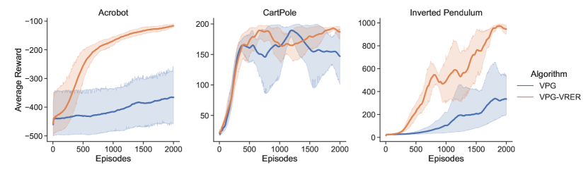
Figure 1: Convergence results for the VPG algorithm with and without using VRER.

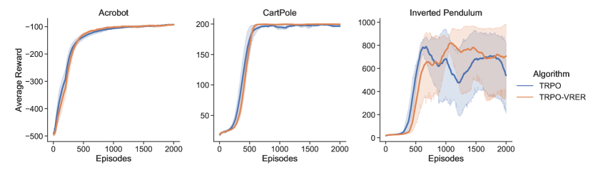
Figure 2: Convergence results for the TRPO algorithm with and without using VRER.

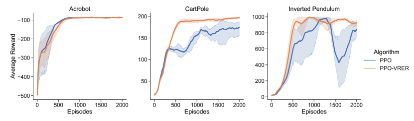
Figure 3: Convergence results for the PPO algorithm with and without using VRER.

We set the same initial learning rate $\eta=0.0003$ for both actor and critic in TPRO and PPO algorithms across all experiments. For VPG, the learning rate of policy model is set to be $\eta=0.0003,0.005$ and 0.0015 respectively for Acrobot, CartPole and Inverted Pendulum problems. The historical sample selection threshold is set to be $c=1.5$ for all VPG experiments. The buffer size is set to $B=400$ except PPO-Acrobot and TRPO-Inverted Pendulum case (for which the buffer size is set to be $B=200$).

Table 2: Performance of the implemented algorithms in terms of average reward over last 1000 training iterations for five different random seeds (same across all algorithms). In bold, the performances of using VRER are statistically significantly different from the baseline algorithm in each task.

Algorithm	Task	Mean	Standard Error	5th Percentile	95th Percentile
PPO	Acrobot	-86.51	0.43	-112.25	-73.50
PPO	CartPole	168.66	1.06	86.98	200.00
PPO	Inverted Pendulum	749.39	10.25	47.35	1000.00
PPO-VRER	Acrobot	-86.95	0.40	-108.64	-74.00
PPO-VRER	CartPole	193.54	0.31	172.98	200.00
PPO-VRER	Inverted Pendulum	941.55	3.37	668.54	1000.00
TRPO	Acrobot	-97.41	0.44	-123.00	-81.25
TRPO	CartPole	197.66	0.26	179.00	200.00
TRPO	Inverted Pendulum	603.77	11.24	13.00	1000.00
TRPO-VRER	Acrobot	-96.93	0.48	-125.00	-79.00
TRPO-VRER	CartPole	199.69	0.05	198.50	200.00
TRPO-VRER	Inverted Pendulum	684.87	9.88	37.50	1000.00
VPG	Acrobot	-381.91	2.99	-500.00	-200.98
VPG	CartPole	163.69	1.37	69.61	200.00
VPG	Inverted Pendulum	256.15	7.68	42.25	947.16
VPG-VRER	Acrobot	-132.11	0.71	-178.14	-99.25
VPG-VRER	CartPole	179.21	0.79	123.11	200.00
VPG-VRER	Inverted Pendulum	779.66	8.08	214.23	1000.00

We plot the mean performance curves and 95% confidence intervals of VPG(-VRER) in Figure 1, and TRPO(-VRER) in Figure 2, and PPO(-VRER) in Figure 3. The results demonstrate that VRER improves the overall performance of the state-of-the-art policy optimization algorithms. For the VPG, we observe a significantly increased convergence speed and stability after using VRER. For the experiments related to PPO algorithm, PPO-VRER shows not only the convergence to better optimum but also faster convergence compared to those without using VRER. In all three cases, the performance improvement for TRPO isn’t as significant as VPG and PPO. In addition, we observe a reduction in the variation of the convergences for those algorithms after implementing VRER.

Table 2 presents the performance (i.e., average total reward, standard error (SE), and percentiles) of all these algorithms over last 1000 episodes, following Schulman et al. (2017) (who considered the average total reward of the last 100 episodes). The efficacy of the proposed VRER is consistently observed across different control tasks. Specifically, in the inverted pendulum task, VRER improves average rewards of PPO by 25.6%, TRPO by 13.4%, and VPG by 204% respectively. In the Acrobot tasks, VRER improves the average reward of VPG from -132.11 to -381.91. In the CartPole tasks, the performance gains from using VRER achieves 14.8% for PPO, 1% for TRPO, and 9.5% for VPG.

6.2 Sensitivity Analysis and Reusing Pattern

In this section, we study the effects of selection constant $c$ and buffer size $B$ on the performance of VRER. Table 3 records the average rewards of TRPO-VRER with different buffer sizes. Overall, the performance of VRER is robust to the selection of buffer size $B$.

Table 3: Sensitivity of buffer sizes. The average reward of TRPO over last 1000 training iterations as a function of the buffer size for 10 random seeds. (mean $\pm$ 95% c.i.).

Buffer Size	Acrobot	CartPole	Inverted Pendulum
$B=200$	-106.72 $\pm$ 6.66	197.25 $\pm$ 1.00	732.92 $\pm$ 216.18
$B=400$	-96.93 $\pm$ 2.80	199.69 $\pm$ 0.19	637.59 $\pm$ 207.50
$B=800$	-153.06 $\pm$ 25.37	195.97 $\pm$ 5.31	615.07 $\pm$ 132.89
$B=1600$	-171.49 $\pm$ 62.99	192.44 $\pm$ 6.51	684.87 $\pm$ 188.62

To better understand how the historical sample selection constant $c$ impacts on the performance of VRER, we conduct additional experiments by using the selection rule (20) (without using any approximation). In all experiments, we run the VPG-VRER algorithm on the CartPole for demonstration. Figure LABEL:sub@fig:_cartpole_sensitivity shows the number of iterations required by VPG-VRER to solve CartPole problem (i.e., the average reward is greater than 195 over 100 consecutive iterations) as a function of average reward with different values of the selection constant $c$. The dashed vertical line indicates the 195 reward. In addition, we record the means and SEs of number of iterations required to solve the CartPole problem with different values of $c$ in Table 4. Overall, these empirical results indicate that the convergence behavior of the VPG-VRER algorithm is robust to the choice of $c$.

Table 4: Sensitivity of selection constants $c$.

Sensitivity	$c$	1.2	1.5	2	4	8
Number of Iterations	Mean	706.44	814.04	918.52	699.32	671.36
	SE	25.98	61.47	49.31	34.91	7.60

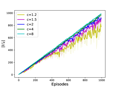
(a) The size of reuse set $|\mathcal{U}_{k}|$ versus episodes.

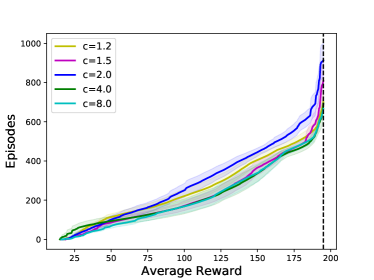
(b) Number of episodes before solving CartPole (average reward is greater than 195).

Figure 4: Sensitivity analyses for selection constant $c$. Result are smoothed by the moving average with a smoothing window width of 100.

Then, we study the impact of the value of selection constant $c$ on the reusing pattern of historical samples. Figure LABEL:sub@fig:_num_reused_model shows the mean and 95% confidence band of the size of reuse set, i.e., $|\mathcal{U}_{k}|$, when $c=1.2,1.5,2,4,8$. It suggests that $|\mathcal{U}_{k}|$ tends to linearly growing with the iteration $k$. Also, as $c$ increases, the number of reused samples tends to increase. The results obtained with $c=2,4,8$ are close to each other. Basically, the value of $c$ determines the tolerance of the variance inflation of ILR policy gradient estimator $\widehat{\nabla\mu}^{ILR}_{i,k}$ relative to the baseline PG policy gradient estimator $\widehat{\nabla\mu}^{PG}_{k}$. When $c$ increases, more historical samples tend to be reused.

6.3 Gradient Variance Reduction

In this section, we present the empirical results to assess the performance of the proposed VRER in terms of reducing the policy gradient estimation variance. This study uses the selection rule (20) with the policy gradient variance estimators (24) and (25). The MLR gradient estimator (16) is used to update the policy parameters in Step 3(b) of Algorithm 1. We record the results of VPG with and without using VRER in Table 5. The original VPG without VRER leads to policy gradient estimators with high variability. By selectively reusing historical transition observations through VRER, the VPG shows a significant reduction in the estimation variance on policy gradient in all three examples. From the results in Table 5, we can see that the total variance of $\widehat{\nabla\mu}^{MLR}_{k}$ is consistently lower than that of $\widehat{\nabla\mu}^{PG}_{k}$ across different tasks over the training process (from episodes 1-500 to 1501-2000).

Table 5: The square root of total gradient variance differences $\sqrt{\left(\mbox{Tr}\left(\widehat{\mbox{Var}}\left(\widehat{\nabla\mu}^{PG}_{k}\right)\right)\right)}-\sqrt{\left(\mbox{Tr}\left(\widehat{\mbox{Var}}\left(\widehat{\nabla\mu}^{MLR}_{k}\right)\right)\right)}$ in four different groups of episodes. (mean $\pm$ 95% c.i.).

	Episode
Task	1-500	501-1000	1001-1500	1501-2000
Acrobot	$276.12\pm 10.12$	$150.84\pm 6.26$	$112.91\pm 4.85$	$95.54\pm 3.92$
CartPole	$118.06\pm 8.10$	$168.06\pm 8.20$	$147.82\pm 6.91$	$136.89\pm 12.17$
Inverted Pendulum	$121.04\pm 23.25$	$537.80\pm 52.69$	$621.87\pm 93.53$	$908.00\pm 89.35$

6.4 Convergence at Fixed Learning Rate

Theorem 2 shows that the PG-VRER can have asymptotic optimization convergence even with a fixed learning rate $\eta_{k}$ if the size of the reuse set $|\mathcal{U}_{k}|$ increases to infinity as iteration $k$ grows. Here, we empirically investigate this property by comparing the convergence behaviors between VPG and VPG-VRER with the fixed learning rate $\eta=0.005,0.01$. To avoid the impact from approximation error of selection rule (31) and (32), in this section, we use the selection rule (20) with the policy gradient variance estimators (24) and (25). The MLR gradient estimator (16) is used for updating the policy parameters in Step 3(b) of Algorithm 1. We also fix the total number of iterations $K=250$ and set the maximum episode length to 100 (it means that the maximum reward is 100).

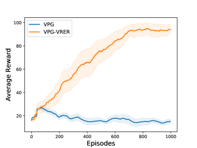
(a) Learning rate $\eta=0.005$.

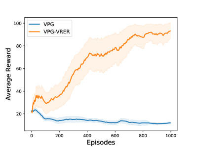
(b) Learning rate $\eta=0.01$

Figure 5: Convergence behaviors of VPG and VPG-VRER with fixed learning rate $\eta$.

The results of mean and $95\%$ confidence interval (CI) of average reward are shown in Figure 5. They indicate that the VPG algorithm (blue line) diverges quickly after few iterations while the average reward of VPG-VRER method (orange line) continues to increase with iterations. Thus, the convergence behavior of VPG-VRER using a fixed stepsize is consistent with the theoretical conclusion in Theorem 2. As the fixed learning rate does not satisfy the Robbins–Monro conditions, the divergence of the VPG is within expectations; see Robbins and Monro (1951).

7 Conclusion

To guide real-time process control in low-data situations, we create a variance reduction experience replay approach to accelerate policy gradient optimization. The proposed selection rule guarantees the variance reduction in the policy gradient estimation through selectively reusing the most relevant historical samples and automatically allocating more weights to those samples that are more likely generated from the target distribution. The VRER approach has strong theoretical grounding since its selection rule is derived from a policy gradient estimation variance reduction criterion, capable of capturing the uncertainty induced by importance sampling. Practically speaking, it is surprisingly simple to apply VRER in most policy gradient optimization approaches as it does not require structural change of original algorithm. Practitioners can implement VRER by adding the selection procedure before training step. Both theoretical and empirical studies show that such variance reduction in gradient estimation can substantially increase the convergence rate of policy gradient methods and enhance the performance of state-of-the-art policy optimization algorithms, such as PPO and TRPO.

Appendix A Experiment Details

In this appendix, we report the hyperparameter values used in the experimental evaluation and some additional results and experiments. In all side-by-side comparison experiments, each pair of baseline algorithm and VRER assisted algorithm were run under same hyperparameter settings. To reproduce the results and check out the implementation details, please visit our open-sourced library: https://github.com/zhenghuazx/vrer_policy_gradient.

A.1 Hyperparameters

• Policy architecture: For discrete action, we adopted a softmax policy: Categorical distributions $\text{Cart}(p_{i})$, where the probabilities $p_{i}=\pi_{\boldsymbol{\theta}}(a_{i}|\boldsymbol{s})$ are modeled by softmax function (for a $m$-dimensional action)

  $$\pi_{\boldsymbol{\theta}}(a_{i}|\boldsymbol{s})=\frac{\exp\left(\phi_{\boldsymbol{\theta}}(\boldsymbol{s},a_{i})\right)}{\sum_{i=1}^{m}\exp\left(\phi_{\boldsymbol{\theta}}(\boldsymbol{s},a_{i}^{\prime})\right)}.$$ (35)

  The mean function $\phi_{\boldsymbol{\theta}}$ is a 2–layers multilayer perceptron (MLP) (32, 32) with bias (activation functions: ReLU for hidden–layers, linear for output layer).

  For continuous actions, we adopted a Gaussian policy: normal distribution $\mathcal{N}(\boldsymbol{a}|\phi_{\boldsymbol{\theta}}(\boldsymbol{s}),I)$, where the mean $\phi_{\boldsymbol{\theta}}$ is a 2–layers multilayer perceptron (MLP) (32, 32) with bias (activation functions: tanh for hidden–layers, linear for output layer the variance is state–independent and parametrized identity matrix).

• Number of macro-replications: 5 (95% c.i.)

• Seeds: 2022,2023,2024,2025,2026 (PPO, PPO-VRER, TRPO and TRPO-VRER); 2021,2022,2023,2024,2025 (VPG and VPG-VRER);

• Policy initialization: glorot uniform initialization for VPG(-VRER) and orthogonal initialization for PPO(-VRER) and TRPO(-VRER)

The VRER related hyperparameters include selection constant $c$, the buffer size $B$, and the number of sampled observations per iteration $n_{0}$.

The PPO(-VRER) hyperparameters are presented in Table 6. The hyperparameter “mini batches" represents the number of mini-batch; “batch size" represents the number of transitions per iteration; “entropy coef" represents the entropy coefficient used for entropy loss calculation; and “Lambda" represents the lambda for the general advantage estimation. The “PPO iterations" hyperparameter ($K_{off}$) represents the maximum number of actor-critic optimizations steps per train step.

Table 6: Hyperparamters for PPO and PPO-VERE

	CartPole	Acrobot	Inverted Pendulum
step size	0.0003	0.0003	0.0003
batch size	512	512	512
clip norm	0.2	0.2	0.2
entropy coef	0.01	0.01	0.01
Lambda	0.95	0.95	0.95
mini batches	128	128	128
PPO iterations	4	4	4
buffer size	400	200	400
$n_{0}$	12	12	12

The TRPO(-VRER) hyperparameters are presented in Table 7. The hyperparameter“cg iterations" represents the gradient conjugation maximum number of iterations per train step; “entropy coef" represents the entropy coefficient used for entropy loss calculation; the “actor/critic iterations" hyperparameter ($K_{off}$) represents the maximum number of actor/critic optimizations steps per train step; and “clip norm" represents the the surrogate clipping coefficient.

Table 7: Hyperparamters for TRPO and TRPO-VERE

	CartPole	Acrobot	Inverted Pendulum
step size	0.0003	0.0003	0.001
batch size	512	512	512
clip norm	0.2	0.2	0.2
entropy coef	0.01	0.01	0.01
mini batches	128	128	128
actor iterations	10	10	10
critic iterations	3	3	3
cg iterations	10	10	10
buffer size	400	400	200
$n_{0}$	12	12	12

Table 8: Hyperparamters for VPG and VPG-VERE

	CartPole	Acrobot	Inverted Pendulum
step size	0.005	0.0003	0.0007
c	1.5	1.5	1.5
buffer size	-	-	-
$n_{0}$	-	-	-

As the VPG is an episode-based algorithm, we use the selection rule (31) with selection constant $c=1.5$ across all experiments. Moveover, in VPG-VRER related experiment runs, we did not use the buffer and thus no buffer size and set $n_{0}=n$ number of randomly sampled observations per iteration; see Table 8. In practice, we recommend users tune the selection rule constant together with the learning rate (step size).

A.2 Runtime Analysis

To better understand the computational complexity of VRER, we present the summary table of runtime in Table 9.

Table 9: Runtime (in minute) of 2000 episodes with a fixed buffer size $B=100$.

	Acrobot		CartPole		Inverted Pendulum
Algorithm	Mean	SE	Mean	SE	Mean	SE
PPO	218.29	12.40	278.62	11.80	5,727.01	329.43
PPOVRER	406.82	64.09	753.34	76.02	7,788.85	241.37
TRPO	292.98	10.64	353.08	12.57	5,526.60	806.29
TRPOVRER	359.53	28.62	627.71	89.51	5,621.70	963.02

A.3 Control Tasks

All control systems are simulated based on the simulation model provided in the Open AI library (Brockman et al., 2016) and PyBullet library (Coumans and Bai, 2021).

CartPole is a pendulum with a center of gravity above its pivot point; see more detailed description in Barto et al. (1983). The goal is to keep the cart-pole balanced by applying appropriate forces to a pivot point under the center of mass and prevent the pendulum from falling over. At any time $t$, the state vector $\boldsymbol{s}_{t}$ for this system is a four dimensional vector having components ${x_{t},\dot{x}_{t},\alpha_{t},\dot{\alpha}_{t}}$ representing position of cart, velocity of cart, angle of pole, and rotation rate of pole respectively. The action $a_{t}$ consists of a force $\overrightarrow{F_{t}}$: left (0) and right (1). Each episode or simulation run terminates if (1) the pole angle is more than 12 degree from the vertical axis; or (2) the cart position is more than 2.4 unit from the centre; or (3) the episode length is greater than 200. The agent receives a reward of 1 for each step taken including the termination step. The problem is considered “solved" if the average reward is greater than 195 over 100 consecutive iterations.

The Acrobot environment is constructed based on Sutton’s work (Sutton, 1995). The system consists of two links connected linearly to form a chain, with one end of the chain fixed. The joint between the two links is actuated. The goal is to apply torques on the actuated joint to swing the free end of the linear chain above a given height while starting from the initial state of hanging downwards. This problem has 3 discrete actions and 6 continuous states. The goal is to have the free end reaching a designated target height in as few steps as possible, and as such all steps that do not reach the goal incur a reward of -1. Achieving the target height results in termination with a reward of 0.

The inverted pendulum system is an example commonly found in control system textbooks and research literature. The objective of the control system is to balance the inverted pendulum by applying a force to the cart that the pendulum is attached to. The problem has one continuous action valued between -1 and 1 and five continuous states. The maximum episode length is 1000; see details in PyBullet library (Coumans and Bai, 2021).

A.4 Confidence Intervals

At each $k$-th iteration, based on the results obtained from $m_{r}$ macro-replications, we represent the estimation uncertainty of the output, denoted by $x_{k}$, by using the 95% confidence bands, $\left(\mu^{m}_{k}-z\cdot\mbox{SE}_{k},\mu^{m}_{k}+z\cdot\mbox{SE}_{k}\right),$ with $z=1.96$, sample mean $\mu^{m}_{k}=\frac{1}{m_{r}}\sum^{m_{r}}_{\ell=1}x_{k,\ell}$, and sample standard error (SE), i.e.,

$$\mbox{SE}_{k}=\frac{1}{\sqrt{(m_{r}-1)m_{r}}}\sqrt{\sum^{m_{r}}_{\ell=1}(x_{k,\ell}-\mu^{m}_{k})^{2}}.$$

In our empirical study, this quantity can be the expected total reward, the size of reuse set $|\mathcal{U}_{k}|$, or the trace of policy gradient estimation variance matrix $\mbox{Tr}(\mbox{Var}[\widehat{\nabla\mu}(\boldsymbol{\theta}_{k})])$). For example, in the convergence plots, we record the averaged total reward $x_{k,\ell}=\frac{1}{n}\sum^{n}_{j=1}R_{\ell}^{(k,j)}$; in the figure of reusing patterns (i.e., Figure LABEL:sub@fig:_num_reused_model), we set $x_{k,\ell}=|\mathcal{U}_{k,\ell}|$, the size of reuse set obtained in the $\ell$-th macro-replication; and lastly we set $x_{k,\ell}$ to be the square root of the total variance or the trace of variance matrix of gradient estimator at the $k$-th iteration and the $\ell$-th macro-replication for Figure 5.

Appendix B Theoretical Analysis and Proofs

B.1 Proof of Lemma 3

Lemma 3 Conditional on $\mathcal{F}_{k}$, the proposed MLR policy gradient estimators are unbiased:

$${\mathbb{E}}\left[\left.\widehat{\nabla\mu}^{MLR}_{k}\right|\mathcal{F}_{k}\right]={\mathbb{E}}\left[\left.g_{k}(\boldsymbol{x})\right|\boldsymbol{\theta}_{k}\right]=\nabla\mu(\boldsymbol{\theta}_{k}).$$

Proof.

We show that the MLR policy gradient estimator listed in (16) is unbiased,

$${\mathbb{E}}\left.\left[\widehat{\nabla\mu}_{k}^{MLR}\right|\mathcal{F}_{k}\right]$$

$$= \int\frac{1}{|\mathcal{U}_{k}|}\sum_{\boldsymbol{\theta}_{i}\in\mathcal{U}_{k}}\frac{\rho_{\boldsymbol{\theta}_{k}}(\boldsymbol{x})}{\frac{1}{|\mathcal{U}_{k}|}\sum_{\boldsymbol{\theta}_{i^{\prime}}\in\mathcal{U}_{k}}\rho_{\boldsymbol{\theta}_{i^{\prime}}}(\boldsymbol{x})}g_{k}(\boldsymbol{x})\rho_{\boldsymbol{\theta}_{i}}(\boldsymbol{x})d\boldsymbol{x}$$

$$= \int\rho_{\boldsymbol{\theta}_{k}}(\boldsymbol{x})g_{k}(\boldsymbol{x})d\boldsymbol{x}$$

$$= {\mathbb{E}}_{\boldsymbol{x}\sim\rho_{\boldsymbol{\theta}_{k}}}\left[g_{k}(\boldsymbol{x})\right].$$

∎

B.2 Proof of Proposition 1

Before proving Lemma 1, we first introduce some additional notations. Denote the $d$-dimensional policy parameter by $\boldsymbol{\theta}=(\theta^{(1)},\ldots,\theta^{(d)})^{\top}\in\mathbb{R}^{d}$. Remember that $g_{k}(\boldsymbol{x})$ denote the scenario-based policy gradient estimate at $\boldsymbol{\theta}_{k}$, and it is a $d$-dimensional vector

$$g_{k}(\boldsymbol{x})=(g_{1},\ldots,g_{d})^{\top}$$

where $g_{i}=\sum^{H}_{t=1}R(\boldsymbol{\tau})\frac{\partial}{\partial\theta^{(i)}}\mbox{log}\pi_{\boldsymbol{\theta}_{k}}({\boldsymbol{a}_{t}|\boldsymbol{s}_{t}})$ for finite horizon and $g_{i}=A^{\pi_{\boldsymbol{\theta}_{k}}}(\boldsymbol{s},\boldsymbol{a})\frac{\partial}{\partial\theta^{(i)}}\mbox{log}\pi_{\boldsymbol{\theta}_{k}}({\boldsymbol{a}_{t}|\boldsymbol{s}_{t}})$ for infinite horizon MDP.

Proposition 1 Conditional on $\mathcal{F}_{k}$, the total variance of the MLR policy gradient estimator is smaller and equal to that of the average ILR policy gradient estimator,

$$\mbox{Tr}\left(\mbox{Var}\left[\left.\widehat{\nabla\mu}^{MLR}_{k}\right|\mathcal{F}_{k}\right]\right)\leq\mbox{Tr}\left(\mbox{Var}\left[\left.{\widehat{\nabla\mu}}^{ILR}_{k}\right|\mathcal{F}_{k}\right]\right).$$

Proof.

Let $\left\{\widetilde{\boldsymbol{x}}^{(i,j)}\sim\rho_{\boldsymbol{\theta}_{k}}(\boldsymbol{x}):\boldsymbol{\theta}_{i}\in\mathcal{U}_{k}~{}~{}\mbox{and}~{}~{}j=1,2,\ldots,n\right\}$ be i.i.d. samples from the mixture distribution $\frac{1}{|\mathcal{U}_{k}|}\sum_{\boldsymbol{\theta}_{i}\in\mathcal{U}_{k}}\rho_{\boldsymbol{\theta}_{i}}(\boldsymbol{x})$ and obtain the policy gradient estimator,

$$\widehat{\nabla\mu}^{Mix}_{k}=\frac{1}{|\mathcal{U}_{k}|}\sum_{\boldsymbol{\theta}_{i}\in\mathcal{U}_{k}}\frac{1}{n}\sum^{n}_{j=1}\left[f_{k}\left(\widetilde{\boldsymbol{x}}^{(i,j)}\right)g_{k}\left(\widetilde{\boldsymbol{x}}^{(i,j)}\right)\right].$$

The estimators $\nabla\mu^{MLR}_{k}$ and $\nabla\mu^{Mix}_{k}$ are similar: the former is a stratified-sampling version of the latter without considering the random sampling of parameters from the reuse set $\mathcal{U}_{k}$. Clearly, $\widehat{\nabla\mu}^{Mix}_{k}$ is unbiased. Therefore, ${\mathbb{E}}\left[\widehat{\nabla\mu}^{MLR}_{k}\right]={\mathbb{E}}\left[\widehat{\nabla\mu}^{Mix}_{k}\right]={\mathbb{E}}_{\boldsymbol{x}\sim\rho_{\boldsymbol{\theta}_{k}}}\left[g_{k}(\boldsymbol{x})\right]$, which equals $\nabla\mu(\boldsymbol{\theta})$ by Lemma 3. By plugging in (15), we have

$$\mbox{Var}\left[\left.\widehat{\nabla\mu}^{ILR}_{k}\right|\mathcal{F}_{k}\right]-\mbox{Var}\left[\left.\widehat{\nabla\mu}^{Mix}_{k}\right|\mathcal{F}_{k}\right]$$ (36)

$$\stackrel{{\scriptstyle(*)}}{{=}} \frac{1}{n}\mbox{Var}\left[\left.\frac{1}{|\mathcal{U}_{k}|}\sum_{\boldsymbol{\theta}_{i}\in\mathcal{U}_{k}}\left[\frac{\rho_{\boldsymbol{\theta}_{k}}(\boldsymbol{x})}{\rho_{\boldsymbol{\theta}_{i}}(\boldsymbol{x})}g_{k}(\boldsymbol{x})\right]\right|\mathcal{F}_{k}\right]$$

$$-\frac{1}{n}\mbox{Var}\left[\left.\frac{1}{|\mathcal{U}_{k}|}\sum_{\boldsymbol{\theta}_{i}\in\mathcal{U}_{k}}\left[\frac{\rho_{\boldsymbol{\theta}_{k}}(\boldsymbol{x})}{\frac{1}{|\mathcal{U}_{k}|}\sum_{\boldsymbol{\theta}_{i}\in\mathcal{U}_{k}}\rho_{\boldsymbol{\theta}_{i}}(\boldsymbol{x})}g_{k}(\boldsymbol{x})\right]\right|\mathcal{F}_{k}\right]$$

$$= \frac{1}{n}\int\frac{1}{|\mathcal{U}_{k}|}\sum_{\boldsymbol{\theta}_{i}\in\mathcal{U}_{k}}\left[\frac{\rho_{\boldsymbol{\theta}_{k}}(\boldsymbol{x})}{\rho_{\boldsymbol{\theta}_{i}}(\boldsymbol{x})}\right]^{2}g_{k}({\boldsymbol{x}})g_{k}(\boldsymbol{x})^{\top}\rho_{\boldsymbol{\theta}_{i}}(\boldsymbol{x})d\boldsymbol{x}$$

$$-\frac{1}{n}\int\left[\frac{|\mathcal{U}_{k}|\rho_{\boldsymbol{\theta}_{k}}(\boldsymbol{x})}{\sum_{\boldsymbol{\theta}_{i}\in\mathcal{U}_{k}}\rho_{\boldsymbol{\theta}_{i}}(\boldsymbol{x})}\right]^{2}g_{k}({\boldsymbol{x}})g_{k}(\boldsymbol{x})^{\top}\left[\frac{1}{|\mathcal{U}_{k}|}\sum_{\boldsymbol{\theta}_{i}\in\mathcal{U}_{k}}\rho_{\boldsymbol{\theta}_{i}}(\boldsymbol{x})\right]d\boldsymbol{x}$$

$$= \frac{1}{n}\int\left[\rho_{\boldsymbol{\theta}_{k}}(\boldsymbol{x})^{2}g_{k}(\boldsymbol{x})g_{k}(\boldsymbol{x})^{\top}\right]\left[\frac{1}{|\mathcal{U}_{k}|}\sum_{\boldsymbol{\theta}_{i}\in\mathcal{U}_{k}}\frac{1}{\rho_{\boldsymbol{\theta}_{i}}(\boldsymbol{x})}-\frac{|\mathcal{U}_{k}|}{\sum_{\boldsymbol{\theta}_{i}\in\mathcal{U}_{k}}\rho_{\boldsymbol{\theta}_{i}}(\boldsymbol{x})}\right]d\boldsymbol{x}$$

Step $(*)$ holds because of the conditional independence of samples $\boldsymbol{x}^{(i,j)}\sim\rho_{\boldsymbol{\theta}_{i}}(\boldsymbol{x})$ with $\boldsymbol{\theta}_{i}\in\mathcal{U}_{k}$ and $j=1,2,...,n$.

Notice that $g_{k}(\boldsymbol{x})g_{k}(\boldsymbol{x})^{\top}=\begin{pmatrix}g_{1}^{2}&g_{1}g_{2}&\ldots&g_{1}g_{d}\\ g_{2}g_{1}&g_{2}^{2}&\ldots&g_{2}g_{d}\\ \vdots&\vdots&\ddots&\vdots\\ g_{1}g_{d}&g_{d}g_{2}&\ldots&g_{d}^{2}\\ \end{pmatrix}$ and also $\mbox{Tr}\left(g_{k}(\boldsymbol{x})g_{k}(\boldsymbol{x})^{\top}\right)=\sum_{i}^{d}g_{i}^{2}=\left\|g_{k}(\boldsymbol{x})\right\|^{2}$. Then the trace of covariance matrix (36) becomes

$$\mbox{Tr}\left(\mbox{Var}\left[\left.\widehat{\nabla\mu}^{ILR}_{k}\right|\mathcal{F}_{k}\right]\right)-\mbox{Tr}\left(\left[\left.\widehat{\nabla\mu}^{Mix}_{k}\right|\mathcal{F}_{k}\right]\right)$$ (37)

$$= \frac{1}{n}\int\left(\rho_{\boldsymbol{\theta}_{k}}(\boldsymbol{x})\left\|g_{k}(\boldsymbol{x})\right\|\right)^{2}\left[\frac{1}{|\mathcal{U}_{k}|}\sum_{\boldsymbol{\theta}_{i}\in\mathcal{U}_{k}}\frac{1}{\rho_{\boldsymbol{\theta}_{i}}(\boldsymbol{x})}-\frac{|\mathcal{U}_{k}|}{\sum_{\boldsymbol{\theta}_{i}\in\mathcal{U}_{k}}\rho_{\boldsymbol{\theta}_{i}}(\boldsymbol{x})}\right]d\boldsymbol{x}$$

$$\geq 0\vspace{-0.1in}$$

which holds due to the well-known inequality between arithmetic and harmonic mean, i.e.,

$$\frac{1}{|\mathcal{U}_{k}|}\sum_{\boldsymbol{\theta}_{i}\in\mathcal{U}_{k}}\frac{1}{\rho_{\boldsymbol{\theta}_{i}}(\boldsymbol{x})}\geq\frac{1}{\frac{1}{|\mathcal{U}_{k}|}\sum_{\boldsymbol{\theta}_{i}\in\mathcal{U}_{k}}\rho_{\boldsymbol{\theta}_{i}}(\boldsymbol{x})}.$$

Next, we observe that $\widehat{\nabla\mu}^{MLR}_{k}$ is a stratified-sampling version of $\widehat{\nabla\mu}^{Mix}_{k}$, with $n$ equal number of samples allocated to each behavioral policy in $\mathcal{U}_{k}$. This means equally weighted strata: the sampling likelihood of the $i$-th stratum is $\rho_{\boldsymbol{\theta}_{i}}(\cdot)$. Therefore, $\mbox{Tr}\left(\mbox{Var}\left[\left.\widehat{\nabla\mu}^{MLR}_{k}\right|\mathcal{F}_{k}\right]\right)\leq\mbox{Tr}\left(\mbox{Var}\left[\left.\widehat{\nabla\mu}^{Mix}_{k}\right|\mathcal{F}_{k}\right]\right)$. Combining (37) leads to the desired result $\mbox{Tr}\left(\mbox{Var}\left[\left.\widehat{\nabla\mu}^{MLR}_{k}\right|\mathcal{F}_{k}\right]\right)\leq\mbox{Tr}\left(\mbox{Var}\left[\left.\widehat{\nabla\mu}^{ILR}_{k}\right|\mathcal{F}_{k}\right]\right)$.

∎

B.3 Proof of Theorems 1

Theorem 1: At the $k$-th iteration with the target distribution $\rho_{\boldsymbol{\theta}_{k}}(\boldsymbol{x})$, the reuse set $\mathcal{U}_{k}$ is created to include the distributions, i.e., $\rho_{\boldsymbol{\theta}_{i}}(\boldsymbol{x})$ with $\boldsymbol{\theta}_{i}\in\mathcal{F}_{k}$, whose ILR policy gradient estimator’s total variance is no greater than $c$ times the total variance of the classical PG estimator for some constant $c>1$. Mathematically,

$$\mbox{Tr}\left(\mbox{Var}\left[\left.\widehat{\nabla\mu}^{ILR}_{i,k}\right|\mathcal{F}_{k}\right]\right)\leq c\mbox{Tr}\left(\mbox{Var}\left[\left.\widehat{\nabla\mu}^{PG}_{k}\right|\boldsymbol{\theta}_{k}\right]\right).$$

Then, based on such reuse set $\mathcal{U}_{k}$, the total variance of the MLR/ILR policy gradient estimators (15) and (16) are no greater than $\frac{c}{|\mathcal{U}_{k}|}$ times the total variance of the PG estimator,

$$\mbox{Tr}\left(\mbox{Var}\left[\left.\widehat{\nabla\mu}^{MLR}_{k}\right|\mathcal{F}_{k}\right]\right)\leq\mbox{Tr}\left(\mbox{Var}\left[\left.\widehat{\nabla\mu}^{ILR}_{k}\right|\mathcal{F}_{k}\right]\right)\leq\frac{c}{|\mathcal{U}_{k}|}\mbox{Tr}\left(\mbox{Var}\left[\left.\widehat{\nabla\mu}^{PG}_{k}\right|\boldsymbol{\theta}_{k}\right]\right).$$

Moreover,

$${\mathbb{E}}\left[\left.\left\|\widehat{\nabla\mu}^{MLR}_{k}\right\|^{2}\right|\mathcal{F}_{k}\right]\leq{\mathbb{E}}\left[\left.\left\|\widehat{\nabla\mu}^{ILR}_{k}\right\|^{2}\right|\mathcal{F}_{k}\right]\leq\frac{c}{|\mathcal{U}_{k}|}{\mathbb{E}}\left[\left.\left\|\widehat{\nabla\mu}^{PG}_{k}\right\|^{2}\right|\boldsymbol{\theta}_{k}\right]+\left(1-\frac{c}{|\mathcal{U}_{k}|}\right)\left\|\nabla\mu(\boldsymbol{\theta}_{k})\right\|^{2}.$$

Proof.

Conditional on $\mathcal{F}_{k}$, by Assumption A.3, the observations $\boldsymbol{x}^{(i,j)}$ for any $\boldsymbol{\theta}_{i}\in\mathcal{U}_{k}$ and $j=1,2,\ldots,n$ are independent. Thus, we have

$$\mbox{Tr}\left(\mbox{Var}\left[\left.\widehat{\nabla\mu}^{MLR}_{k}\right|\mathcal{F}_{k}\right]\right)\leq\mbox{Tr}\left(\mbox{Var}\left[\left.\widehat{\nabla\mu}^{ILR}_{k}\right|\mathcal{F}_{k}\right]\right)$$

$$= \frac{1}{|\mathcal{U}_{k}|^{2}}\sum_{\boldsymbol{\theta}_{i}\in\mathcal{U}_{k}}\mbox{Tr}\left(\mbox{Var}\left[\left.\widehat{\nabla\mu}^{ILR}_{i,k}\right|\mathcal{F}_{k}\right]\right)$$

$$\leq \frac{c}{|\mathcal{U}_{k}|^{2}}\sum_{\boldsymbol{\theta}_{i}\in\mathcal{U}_{k}}\mbox{Tr}\left(\mbox{Var}\left[\left.\widehat{\nabla\mu}^{PG}_{k}\right|\boldsymbol{\theta}_{k}\right]\right)$$ (39)

$$= \frac{c}{|\mathcal{U}_{k}|}\mbox{Tr}\left(\mbox{Var}\left[\left.\widehat{\nabla\mu}^{PG}_{k}\right|\boldsymbol{\theta}_{k}\right]\right)$$ (40)

where inequality (B.3) follows Proposition 1 and (39) holds because of selection rule (20). Thus, (21) is proved. Then, we have

$$\mbox{Tr}\left(\mbox{Var}\left[\left.\widehat{\nabla\mu}^{MLR}_{k}\right|\mathcal{F}_{k}\right]\right)$$ (41)

$$= \mbox{Tr}\left({\mathbb{E}}\left[\left.\left(\widehat{\nabla\mu}^{MLR}_{k}\right)\left(\widehat{\nabla\mu}^{MLR}_{k}\right)^{\top}\right|\mathcal{F}_{k}\right]-{\mathbb{E}}\left[\left.\widehat{\nabla\mu}^{MLR}_{k}\right|\mathcal{F}_{k}\right]{\mathbb{E}}\left[\left.\widehat{\nabla\mu}^{MLR}_{k}\right|\mathcal{F}_{k}\right]^{\top}\right)$$

$$= {\mathbb{E}}\left[\left.\left\|\widehat{\nabla\mu}^{MLR}_{k}\right\|^{2}\right|\mathcal{F}_{k}\right]-\left\|{\mathbb{E}}\left[\left.\widehat{\nabla\mu}^{MLR}_{k}\right|\mathcal{F}_{k}\right]\right\|^{2}$$

$$= {\mathbb{E}}\left[\left.\left\|\widehat{\nabla\mu}^{MLR}_{k}\right\|^{2}\right|\mathcal{F}_{k}\right]-\left\|\nabla\mu(\boldsymbol{\theta}_{k})\right\|^{2}$$

where (41) follows because the MLR policy gradient estimator $\widehat{\nabla\mu}^{MLR}_{k}$ is unbiased. Similarly, we have

$$\mbox{Tr}\left(\mbox{Var}\left[\left.\widehat{\nabla\mu}^{PG}_{k}\right|\boldsymbol{\theta}_{k}\right]\right)={\mathbb{E}}\left[\left.\left\|\widehat{\nabla\mu}^{PG}_{k}\right\|^{2}\right|\boldsymbol{\theta}_{k}\right]-\left\|\nabla\mu(\boldsymbol{\theta}_{k})\right\|^{2}.$$ (42)

$$\mbox{Tr}\left(\mbox{Var}\left[\left.\widehat{\nabla\mu}^{ILR}_{k}\right|\boldsymbol{\theta}_{k}\right]\right)={\mathbb{E}}\left[\left.\left\|\widehat{\nabla\mu}^{ILR}_{k}\right\|^{2}\right|\boldsymbol{\theta}_{k}\right]-\left\|\nabla\mu(\boldsymbol{\theta}_{k})\right\|^{2}.$$ (43)

where the equalities hold due to the unbiasedness of $\widehat{\nabla\mu}^{PG}_{k}$ and $\widehat{\nabla\mu}^{ILR}_{k}$ Then with Proposition 1 and (40)–(42), we can show

$${\mathbb{E}}\left[\left.\left\|\widehat{\nabla\mu}^{MLR}_{k}\right\|^{2}\right|\mathcal{F}_{k}\right]\leq{\mathbb{E}}\left[\left.\left\|\widehat{\nabla\mu}^{ILR}_{k}\right\|^{2}\right|\mathcal{F}_{k}\right]\leq\frac{c}{|\mathcal{U}_{k}|}{\mathbb{E}}\left[\left.\left\|\widehat{\nabla\mu}^{PG}_{k}\right\|^{2}\right|\boldsymbol{\theta}_{k}\right]+\left(1-\frac{c}{|\mathcal{U}_{k}|}\right)\left\|\nabla\mu(\boldsymbol{\theta}_{k})\right\|^{2}.$$ (44)

It completes the proof. ∎

B.4 Proof of Lemma 4

Lemma 4 Suppose that Assumption A.1, A.2 and A.3 hold. For a clipped likelihood ratio based policy gradient estimator $\widehat{\nabla\mu}^{CLR}_{k}$, with a finite clipping threshold $U_{f}>1$, the bias and the variance of the CLR estimator can be upper bounded as

$$\left\|{\mathbb{E}}\left[\widehat{\nabla\mu}^{CLR}_{k}\right]-\nabla\mu(\boldsymbol{\theta}_{k})\right\|\leq Z(k),\vspace{-0.1in}$$

$$\mbox{Tr}\left(\mbox{Var}\left[\left.\widehat{\nabla\mu}^{CLR}_{k}\right|\mathcal{F}_{k}\right]\right)\leq\mbox{Tr}\left(\mbox{Var}\left[\left.\widehat{\nabla\mu}^{ILR}_{k}\right|\mathcal{F}_{k}\right]\right)+\frac{1}{n|\mathcal{U}_{k}|}\left\|\nabla\mu(\boldsymbol{\theta}_{k})\right\|^{2}.\vspace{-0.1in}$$

where $Z(k)=\frac{M}{|\mathcal{U}_{k}|}\sum_{{\boldsymbol{\theta}_{i}}\in\mathcal{U}_{k}}{\mathbb{E}}_{k}\left[\mathbbm{1}\left\{{f}_{i,k}(\boldsymbol{x})>U_{f}\right\}\right]$ and $M$ is the bound defined in Lemma 2

Proof.

Let ${\mathbb{E}}_{k}[\cdot]={\mathbb{E}}[\cdot|\mathcal{F}_{k}]$ and $M=\max(\frac{2U_{\Theta}U_{r}}{1-\gamma},H^{2}U_{\Theta}U_{r})$ is the bound of stochastic gradient estimate. Remember $f_{i,k}(\boldsymbol{x})=\frac{\rho_{\boldsymbol{\theta}_{k}}(\boldsymbol{x})}{\rho_{\boldsymbol{\theta}_{i}}(\boldsymbol{x})}$. Let $\breve{f}_{i,k}(\boldsymbol{x})=\min\left(\frac{\rho_{\boldsymbol{\theta}_{k}}(\boldsymbol{x})}{\rho_{\boldsymbol{\theta}_{i}}(\boldsymbol{x})},U_{f}\right)$. Then we have

$$\left\|{\mathbb{E}}\left[\widehat{\nabla\mu}_{k}^{CLR}\right]-\nabla\mu(\boldsymbol{\theta}_{k})\right\|=\left\|{\mathbb{E}}\left[\widehat{\nabla\mu}_{k}^{CLR}\right]-{\mathbb{E}}_{i}\left[\widehat{\nabla\mu}_{k}^{ILR}\right]\right\|$$

$$=\left\|{\mathbb{E}}\left[\frac{1}{|\mathcal{U}_{k}|n}\sum_{{\boldsymbol{\theta}_{i}}\in\mathcal{U}_{k}}\sum^{n}_{j=1}\left(\frac{\rho_{\boldsymbol{\theta}_{k}}(\boldsymbol{x}^{(i,j)})}{\rho_{\boldsymbol{\theta}_{i}}(\boldsymbol{x}^{(i,j)})}-\min\left(U_{f},\frac{\rho_{\boldsymbol{\theta}_{k}}(\boldsymbol{x}^{(i,j)})}{\rho_{\boldsymbol{\theta}_{i}}(\boldsymbol{x}^{(i,j)})}\right)\right)g_{k}\left(\boldsymbol{x}^{(i,j)}\right)\right]\right\|$$

$$\leq\frac{1}{|\mathcal{U}_{k}|}\sum_{{\boldsymbol{\theta}_{i}}\in\mathcal{U}_{k}}\left\|{\mathbb{E}}_{i}\left[\left({f}_{i,k}(\boldsymbol{x})-\breve{f}_{i,k}(\boldsymbol{x})\right)g_{k}\left(\boldsymbol{x}\right)\right]\right\|$$ (45)

$$=\frac{1}{|\mathcal{U}_{k}|}\sum_{{\boldsymbol{\theta}_{i}}\in\mathcal{U}_{k}}\|{\mathbb{E}}_{i}\left[\left({f}_{i,k}(\boldsymbol{x})-U_{f}\right)g_{k}(\boldsymbol{x})\mathbbm{1}\left\{{f}_{i,k}(\boldsymbol{x})>U_{f}\right\}\right]\|$$ (46)

$$\leq\frac{M}{|\mathcal{U}_{k}|}\sum_{{\boldsymbol{\theta}_{i}}\in\mathcal{U}_{k}}{\mathbb{E}}_{i}\left[\left|{f}_{i,k}(\boldsymbol{x})-U_{f}\right|\mathbbm{1}\left\{{f}_{i,k}(\boldsymbol{x})>U_{f}\right\}\right]$$ (47)

$$\leq\frac{M}{|\mathcal{U}_{k}|}\sum_{{\boldsymbol{\theta}_{i}}\in\mathcal{U}_{k}}{\mathbb{E}}_{i}\left[{f}_{i,k}(\boldsymbol{x})\mathbbm{1}\left\{{f}_{i,k}(\boldsymbol{x})>U_{f}\right\}\right]$$ (48)

$$\leq\frac{M}{|\mathcal{U}_{k}|}\sum_{{\boldsymbol{\theta}_{i}}\in\mathcal{U}_{k}}{\mathbb{E}}_{k}\left[\mathbbm{1}\left\{{f}_{i,k}(\boldsymbol{x})>U_{f}\right\}\right]$$

where step (45) follows triangle inequality, step (46) follows from observing that the weight difference is either zero or $U_{f}$ based on whether $\frac{\rho_{\boldsymbol{\theta}_{k}}(\boldsymbol{x})}{\rho_{\boldsymbol{\theta}_{i}}(\boldsymbol{x})}>U_{f}$, and step (47) follows by applying Hölder’s inequality and Lemma 2, step (48) is obtained by observing that under the indicator function we have that ${f}_{i,k}(\boldsymbol{x})>U_{f}$.

Then, we prove the bound of total variance,

$$\mbox{Tr}\left(\mbox{Var}\left[\left.\widehat{\nabla\mu}^{CLR}_{k}\right|\mathcal{F}_{k}\right]\right)=\mbox{Tr}\left(\mbox{Var}\left[\left.\frac{1}{|\mathcal{U}_{k}|n}\sum_{{\boldsymbol{\theta}_{i}}\in\mathcal{U}_{k}}\sum^{n}_{j=1}\min\left(\frac{\rho_{\boldsymbol{\theta}_{k}}(\boldsymbol{x}^{(i,j)})}{\rho_{\boldsymbol{\theta}_{i}}(\boldsymbol{x}^{(i,j)})},U_{f}\right)g_{k}\left(\boldsymbol{x}^{(i,j)}\right)\right|\mathcal{F}_{k}\right]\right)$$

$$=\frac{1}{n|\mathcal{U}_{k}|}\mbox{Tr}\left(\mbox{Var}\left[\left.\min\left(\frac{\rho_{\boldsymbol{\theta}_{k}}(\boldsymbol{x})}{\rho_{\boldsymbol{\theta}_{i}}(\boldsymbol{x})},U_{f}\right)g_{k}\left(\boldsymbol{x}\right)\right|\mathcal{F}_{k}\right]\right)$$

$$=\frac{1}{n|\mathcal{U}_{k}|}\left({\mathbb{E}}_{i}\left[\left\|\min\left(\frac{\rho_{\boldsymbol{\theta}_{k}}(\boldsymbol{x})}{\rho_{\boldsymbol{\theta}_{i}}(\boldsymbol{x})},U_{f}\right)g_{k}\left(\boldsymbol{x}\right)\right\|^{2}\right]-\left\|{\mathbb{E}}_{i}\left[\min\left(\frac{\rho_{\boldsymbol{\theta}_{k}}(\boldsymbol{x})}{\rho_{\boldsymbol{\theta}_{i}}(\boldsymbol{x})},U_{f}\right)g_{k}\left(\boldsymbol{x}\right)\right]\right\|^{2}\right)$$

$$=\frac{1}{n|\mathcal{U}_{k}|}\left({\mathbb{E}}_{i}\left[\min\left(\frac{\rho_{\boldsymbol{\theta}_{k}}(\boldsymbol{x})}{\rho_{\boldsymbol{\theta}_{i}}(\boldsymbol{x})},U_{f}\right)^{2}\left\|g_{k}\left(\boldsymbol{x}\right)\right\|^{2}\right]-\left\|{\mathbb{E}}_{i}\left[\min\left(\frac{\rho_{\boldsymbol{\theta}_{k}}(\boldsymbol{x})}{\rho_{\boldsymbol{\theta}_{i}}(\boldsymbol{x})},U_{f}\right)g_{k}\left(\boldsymbol{x}\right)\right]\right\|^{2}\right)$$

$$\leq\frac{1}{n|\mathcal{U}_{k}|}{\mathbb{E}}_{i}\left[\left(\frac{\rho_{\boldsymbol{\theta}_{k}}(\boldsymbol{x})}{\rho_{\boldsymbol{\theta}_{i}}(\boldsymbol{x})}\right)^{2}\left\|g_{k}\left(\boldsymbol{x}\right)\right\|^{2}\right]$$

$$\leq\frac{1}{n|\mathcal{U}_{k}|}\left({\mathbb{E}}_{i}\left[{f}_{i,k}^{2}(\boldsymbol{x})\left\|g_{k}\left(\boldsymbol{x}\right)\right\|^{2}\right]-\left\|{\mathbb{E}}_{i}\left[{f}_{i,k}(\boldsymbol{x})g_{k}\left(\boldsymbol{x}\right)\right]\right\|^{2}+\left\|{\mathbb{E}}_{i}\left[{f}_{i,k}(\boldsymbol{x})g_{k}\left(\boldsymbol{x}\right)\right]\right\|^{2}\right)$$

$$=\mbox{Tr}\left(\mbox{Var}\left[\left.\widehat{\nabla\mu}^{ILR}_{k}\right|\mathcal{F}_{k}\right]\right)+\frac{1}{n|\mathcal{U}_{k}|}\left\|{\mathbb{E}}_{k}\left[g_{k}\left(\boldsymbol{x}\right)\right]\right\|^{2}.$$

Then the unbiasedness $\left\|{\mathbb{E}}_{k}\left[g_{k}\left(\boldsymbol{x}\right)\right]\right\|=\left\|\nabla\mu(\boldsymbol{\theta}_{k})\right\|$ gives the result stated in Lemma 4 ∎

B.5 Proof of Corollary 1

Corollary 1 At the $k$-th iteration with the target distribution $\rho_{\boldsymbol{\theta}_{k}}(\boldsymbol{x})$, we apply the selection rule from Theorem 1. Then, based on such reuse set $\mathcal{U}_{k}$, we have the following bound

$${\mathbb{E}}\left[\left.\left\|\widehat{\nabla\mu}^{CLR}_{k}\right\|^{2}\right|\mathcal{F}_{k}\right]\leq\frac{c}{|\mathcal{U}_{k}|}{\mathbb{E}}\left[\left.\left\|\widehat{\nabla\mu}^{PG}_{k}\right\|^{2}\right|\boldsymbol{\theta}_{k}\right]+(8+\frac{1}{n|\mathcal{U}_{k}|}-\frac{c}{|\mathcal{U}_{k}|})\|\nabla\mu(\boldsymbol{\theta}_{k})\|+8\sigma^{2}.$$

Proof.

For CLR policy gradient estimator, we have

$$\mbox{Tr}\left(\mbox{Var}\left[\left.\widehat{\nabla\mu}^{CLR}_{k}\right|\mathcal{F}_{k}\right]\right)-\frac{1}{n|\mathcal{U}_{k}|}\|\nabla\mu(\boldsymbol{\theta}_{k})\|$$ (49)

$$\leq \mbox{Tr}\left(\mbox{Var}\left[\left.\widehat{\nabla\mu}^{ILR}_{k}\right|\mathcal{F}_{k}\right]\right)$$

$$\leq \frac{c}{|\mathcal{U}_{k}|}\mbox{Tr}\left(\mbox{Var}\left[\left.\widehat{\nabla\mu}^{PG}_{k}\right|\boldsymbol{\theta}_{k}\right]\right)$$ (50)

where (49) follows by applying Lemma 4 and (50) follows by applying (39)-(40). Then

$$\mbox{Tr}\left(\mbox{Var}\left[\left.\widehat{\nabla\mu}^{CLR}_{k}\right|\mathcal{F}_{k}\right]\right)$$ (51)

$$= \mbox{Tr}\left({\mathbb{E}}\left[\left.\left(\widehat{\nabla\mu}^{CLR}_{k}\right)\left(\widehat{\nabla\mu}^{CLR}_{k}\right)^{\top}\right|\mathcal{F}_{k}\right]-{\mathbb{E}}\left[\left.\widehat{\nabla\mu}^{CLR}_{k}\right|\mathcal{F}_{k}\right]{\mathbb{E}}\left[\left.\widehat{\nabla\mu}^{CLR}_{k}\right|\mathcal{F}_{k}\right]^{\top}\right)$$

$$= {\mathbb{E}}\left[\left.\left\|\widehat{\nabla\mu}^{CLR}_{k}\right\|^{2}\right|\mathcal{F}_{k}\right]-\left\|{\mathbb{E}}\left[\left.\widehat{\nabla\mu}^{CLR}_{k}\right|\mathcal{F}_{k}\right]\right\|^{2}.$$

Rearranging the equality (51) leads to

$${\mathbb{E}}\left[\left.\left\|\widehat{\nabla\mu}^{CLR}_{k}\right\|^{2}\right|\mathcal{F}_{k}\right]=\left\|{\mathbb{E}}\left[\left.\widehat{\nabla\mu}^{CLR}_{k}\right|\mathcal{F}_{k}\right]\right\|^{2}+\mbox{Tr}\left(\mbox{Var}\left[\left.\widehat{\nabla\mu}^{CLR}_{k}\right|\mathcal{F}_{k}\right]\right)$$

$$\leq 8\|\nabla\mu(\boldsymbol{\theta}_{k})\|^{2}+8\sigma^{2}+\frac{c}{|\mathcal{U}_{k}|}\mbox{Tr}\left(\mbox{Var}\left[\left.\widehat{\nabla\mu}^{PG}_{k}\right|\boldsymbol{\theta}_{k}\right]\right)+\frac{1}{n|\mathcal{U}_{k}|}\|\nabla\mu(\boldsymbol{\theta}_{k})\|$$ (52)

$$=8\|\nabla\mu(\boldsymbol{\theta}_{k})\|^{2}+8\sigma^{2}+\frac{c}{|\mathcal{U}_{k}|}\left({\mathbb{E}}\left[\left.\left\|\widehat{\nabla\mu}^{PG}_{k}\right\|^{2}\right|\boldsymbol{\theta}_{k}\right]-\left\|\nabla\mu(\boldsymbol{\theta}_{k})\right\|^{2}\right)+\frac{1}{n|\mathcal{U}_{k}|}\|\nabla\mu(\boldsymbol{\theta}_{k})\|$$ (53)

$$=\frac{c}{|\mathcal{U}_{k}|}{\mathbb{E}}\left[\left.\left\|\widehat{\nabla\mu}^{PG}_{k}\right\|^{2}\right|\boldsymbol{\theta}_{k}\right]+(8+\frac{1}{n|\mathcal{U}_{k}|}-\frac{c}{|\mathcal{U}_{k}|})\|\nabla\mu(\boldsymbol{\theta}_{k})\|+8\sigma^{2}$$

where (52) follows by applying Lemma 4 and (53) follows by applying (42). ∎

B.6 Proof of Proposition 2

Lemma 7.

(DeGroot and Schervish, 2012, Theorem 8.7.1) The covariance estimator

$$\widehat{\mbox{Var}}(X)=\frac{1}{n-1}(X_{i}-\bar{X})(X_{i}-\bar{X})$$

is an unbiased estimator of the covariance $\mbox{Cov}(X,X)=\mbox{Var}(X)$ where $\bar{X}=\frac{1}{n}\sum^{n}_{i=1}X_{i}$ and independent samples $\{X_{i}:i=1,\ldots,n\}$ have same mean ${\mathbb{E}}[X_{i}]={\mathbb{E}}[X]$ for all $i=1,2,\ldots,n$.

Proposition 2. Given $\mathcal{F}_{k}$, the policy gradient variance estimators $\widehat{\mbox{Var}}\left[\left.\widehat{\nabla\mu}^{PG}_{k}\right|\boldsymbol{\theta}_{k}\right]$ in (24) and $\widehat{\mbox{Var}}\left[\left.\widehat{\nabla\mu}^{ILR}_{i,k}\right|\mathcal{F}_{k}\right]$ in (25) are unbiased.

Proof.

We have derived the ILR gradient estimator and its sample covariance matrix

$$\widehat{\nabla\mu}^{ILR}_{k}=\frac{1}{n}\sum_{j=1}^{n}\widehat{\nabla\mu}^{ILR}_{k,j}\quad\mbox{ with }\quad\widehat{\nabla\mu}^{ILR}_{k,j}=\frac{1}{|\mathcal{U}_{k}|}\sum_{\boldsymbol{\theta}_{i}\in\mathcal{U}_{k}}f_{k}\left(\boldsymbol{x}^{(i,j)}\right)g_{k}\left(\boldsymbol{x}^{(i,j)}\right),\mbox{and}$$

$$\widehat{\mbox{Var}}\left[\left.\widehat{\nabla\mu}^{ILR}_{i,k}\right|\mathcal{F}_{k}\right]=\frac{1}{n-1}\sum^{n}_{j=1}\widehat{\sigma}_{i,j}\widehat{\sigma}_{i,j}^{\top}$$

where $\widehat{\sigma}_{i,j}=\left[X_{j}-\bar{X}\right]$ where $X_{j}=\frac{\rho_{\boldsymbol{\theta}_{k}}(\boldsymbol{x}^{(i,j)})}{\rho_{\boldsymbol{\theta}_{i}}(\boldsymbol{x}^{(i,j)})}g_{k}\left(\boldsymbol{x}^{(i,j)}\right)$ and $\bar{X}=\widehat{\nabla\mu}^{ILR}_{i,k}$. Due to the unbiasedness, we also have ${\mathbb{E}}\left[\left.\frac{\rho_{\boldsymbol{\theta}_{k}}(\boldsymbol{x}^{(i,j)})}{\rho_{\boldsymbol{\theta}_{i}}(\boldsymbol{x}^{(i,j)})}g_{k}\left(\boldsymbol{x}^{(i,j)}\right)\right|\mathcal{F}_{k}\right]={\mathbb{E}}\left[\left.\widehat{\nabla\mu}^{ILR}_{i,k}\right|\mathcal{F}_{k}\right]=\nabla\mu(\boldsymbol{\theta}_{k})$ . Given $\mathcal{U}_{k}$, we have $X_{j}$ is conditional independent with $X_{j^{\prime}}$ for any $j\neq j^{\prime}$ (Assumption A.3). The unbiasedness of estimator $\widehat{\mbox{Var}}\left[\left.\widehat{\nabla\mu}^{ILR}_{k}\right|\mathcal{F}_{k}\right]$ immediately follows Lemma 7. The unbiasedness of the policy gradient variance estimators $\widehat{\mbox{Var}}\left[\left.\widehat{\nabla\mu}^{PG}_{k}\right|\boldsymbol{\theta}_{k}\right]$ can be proven in the similar way. ∎

B.7 Proof of Theorem 2 and 4

Lemma 8.

Suppose that Assumption A.1 holds. For any feasible policy parameters $\boldsymbol{\theta}\in\mathbb{R}^{d}$, we have ${\mathbb{E}}[\|\widehat{\nabla\mu}^{PG}(\boldsymbol{\theta})\|^{2}]\leq 2\|\nabla\mu(\boldsymbol{\theta})\|^{2}+2\sigma^{2}$.

Proof.

We proceed by using Assumption A.1

$${\mathbb{E}}\left[\left\|\widehat{\nabla\mu}^{PG}(\boldsymbol{\theta})\right\|^{2}\right] = {\mathbb{E}}\left[\left\|\widehat{\nabla\mu}^{PG}(\boldsymbol{\theta})-\nabla\mu(\boldsymbol{\theta})+\nabla\mu(\boldsymbol{\theta})\right\|^{2}\right]$$ (54)

$$\leq {\mathbb{E}}\left[\left(\left\|\widehat{\nabla\mu}^{PG}(\boldsymbol{\theta})-\nabla\mu(\boldsymbol{\theta})\right\|+\left\|\nabla\mu(\boldsymbol{\theta})\right\|\right)^{2}\right]$$

$$\leq 2{\mathbb{E}}\left[\|\widehat{\nabla\mu}^{PG}(\boldsymbol{\theta})-\nabla\mu(\boldsymbol{\theta})\|^{2}+\left\|\nabla\mu(\boldsymbol{\theta})\right\|^{2}\right]$$

$$\leq 2{\mathbb{E}}\left[\left\|\nabla\mu(\boldsymbol{\theta})\right\|^{2}\right]+2\sigma^{2}$$ (55)

where (54) follows Cauchy–Schwarz inequality and (55) is obtained by applying Assumption A.1. This completes the proof. ∎

Theorem 2 Suppose Assumptions A.1, A.2 and A.3 hold. Let $\eta_{k}$ denote the learning rate used in the $k$-th iteration and $U_{\mu}$ is the bound of objective. If we the ILR and MLR policy gradient estimators in Algorithm 1, We have

$$\frac{1}{K}\sum_{k=1}^{K}{\mathbb{E}}\left[\|\nabla\mu(\boldsymbol{\theta}_{k})\|^{2}\right]\leq\frac{\frac{4}{\eta_{K}}U_{\mu}-\frac{2}{\eta_{1}}\mu\left(\boldsymbol{\theta}_{1}\right)+4cL\sigma^{2}\sum_{k=1}^{K}\frac{\eta_{k}}{|\mathcal{U}_{k}|}}{K},$$

where $\sigma$ and $L$ are the bounds defined in Assumptions A.1 and Lemma 1, and $c$ is the selection constant defined in Theorems 1.

Proof.

Lemma 1 implies the L-Lipschitz property, $|\mu(\boldsymbol{\theta}_{k})-\mu(\boldsymbol{\theta}_{k+1})-\langle\nabla\mu(\boldsymbol{\theta}_{k}),\boldsymbol{\theta}_{k}-\boldsymbol{\theta}_{k+1}\rangle|\leq L\lVert\boldsymbol{\theta}_{k+1}-\boldsymbol{\theta}_{k}\rVert^{2}$ (Nesterov (2003), Lemma 1.2.3). It gives $\mu(\boldsymbol{\theta}_{k})-\mu(\boldsymbol{\theta}_{k+1})\leq\langle\nabla\mu(\boldsymbol{\theta}_{k}),\boldsymbol{\theta}_{k}-\boldsymbol{\theta}_{k+1}\rangle+L\|\boldsymbol{\theta}_{k+1}-\boldsymbol{\theta}_{k}\|^{2}$.

By applying the policy parameter update implemented in the proposed algorithm $\boldsymbol{\theta}_{k+1}=\boldsymbol{\theta}_{k}+\eta_{k}\widehat{\nabla\mu}^{LR}_{k}$, where $\widehat{\nabla\mu}^{LR}_{k}$ represents either MLR policy gradient estimator $\widehat{\nabla\mu}^{MLR}_{k}$ or ILR policy gradient estimator $\widehat{\nabla\mu}^{ILR}_{k}$, we have

$$\mu(\boldsymbol{\theta}_{k})-\mu(\boldsymbol{\theta}_{k+1})\leq-\left\langle\nabla\mu(\boldsymbol{\theta}_{k}),\eta_{k}\widehat{\nabla\mu}^{LR}_{k}(\boldsymbol{\theta}_{k})\right\rangle+L\|\boldsymbol{\theta}_{k+1}-\boldsymbol{\theta}_{k}\|^{2}.$$ (56)

Taking the expectation of $\left\langle\nabla\mu(\boldsymbol{\theta}_{k}),\eta_{k}\widehat{\nabla\mu}^{LR}_{k}(\boldsymbol{\theta}_{k})\right\rangle$ conditioning on $\mathcal{U}_{k}$, we have that

$${\mathbb{E}}\left[\left.\left\langle\nabla\mu(\boldsymbol{\theta}_{k}),\eta_{k}\widehat{\nabla\mu}^{LR}_{k}(\boldsymbol{\theta}_{k})\right\rangle\right|\mathcal{F}_{k}\right]=\eta_{k}\left\langle\nabla\mu(\boldsymbol{\theta}_{k}),{\mathbb{E}}\left[\left.\widehat{\nabla\mu}^{LR}_{k}(\boldsymbol{\theta}_{k})\right|\mathcal{F}_{k}\right]\right\rangle\stackrel{{\scriptstyle(*)}}{{=}}\eta_{k}\left\|\nabla\mu(\boldsymbol{\theta}_{k})\right\|^{2}$$ (57)

where step $(*)$ follows because the ILR/MLR estimator $\widehat{\nabla\mu}^{LR}_{k}(\boldsymbol{\theta}_{k})$ is conditionally unbiased (Lemma 3). Taking the expectation of $\left\|\boldsymbol{\theta}_{k+1}-\boldsymbol{\theta}_{k}\right\|^{2}$ conditioning on $\mathcal{F}_{k}$ and then applying Theorem 1, we have

$${\mathbb{E}}\left[\left.\left\|\boldsymbol{\theta}_{k+1}-\boldsymbol{\theta}_{k}\right\|^{2}\right|\mathcal{F}_{k}\right] = \eta_{k}^{2}{\mathbb{E}}\left[\left.\left\|\widehat{\nabla\mu}^{LR}_{k}\right\|^{2}\right|\mathcal{F}_{k}\right]$$ (58)

$$\leq \eta_{k}^{2}\frac{c}{|\mathcal{U}_{k}|}{\mathbb{E}}\left[\left.\left\|\widehat{\nabla\mu}^{PG}_{k}\right\|^{2}\right|\boldsymbol{\theta}_{k}\right]+\eta_{k}^{2}\left(1-\frac{c}{|\mathcal{U}_{k}|}\right)\|\nabla\mu(\boldsymbol{\theta}_{k})\|^{2}.$$

Then by taking the unconditional expectation of both sides of (56) and plugging in (57) and (58), we have

$${\mathbb{E}}\left[\mu(\boldsymbol{\theta}_{k})\right]-{\mathbb{E}}\left[\mu(\boldsymbol{\theta}_{k+1})\right]$$ (59)

$$\leq -{\eta_{k}}{\mathbb{E}}\left[\|\nabla\mu(\boldsymbol{\theta}_{k})\|^{2}\right]+L\eta_{k}^{2}\frac{c}{|\mathcal{U}_{k}|}{\mathbb{E}}\left[\left\|\widehat{\nabla\mu}^{PG}_{k}\right\|^{2}\right]+L\eta_{k}^{2}\left(1-\frac{c}{|\mathcal{U}_{k}|}\right){\mathbb{E}}\left[\|\nabla\mu(\boldsymbol{\theta}_{k})\|^{2}\right]$$

$$\leq -{\eta_{k}}{\mathbb{E}}\left[\|\nabla\mu(\boldsymbol{\theta}_{k})\|^{2}\right]+L\eta_{k}^{2}\frac{c}{|\mathcal{U}_{k}|}{\mathbb{E}}\left[\left\|\widehat{\nabla\mu}^{PG}_{k}\right\|^{2}\right]+L\eta_{k}^{2}{\mathbb{E}}\left[\|\nabla\mu(\boldsymbol{\theta}_{k})\|^{2}\right]$$

Rearranging both sides of (59) gives

$$(\eta_{k}-L\eta_{k}^{2}){\mathbb{E}}\left[\|\nabla\mu(\boldsymbol{\theta}_{k})\|^{2}\right]\leq\left({\mathbb{E}}\left[\mu(\boldsymbol{\theta}_{k+1})\right]-{\mathbb{E}}\left[\mu(\boldsymbol{\theta}_{k})\right]\right)+L\eta_{k}^{2}\frac{c}{|\mathcal{U}_{k}|}{\mathbb{E}}\left[\left\|\widehat{\nabla\mu}^{PG}_{k}\right\|^{2}\right].$$ (60)

By applying Lemma 8, i.e., ${\mathbb{E}}\left[\|\widehat{\mu}^{PG}_{k}\|^{2}\right]\leq 2{\mathbb{E}}\left[\|\nabla\mu(\boldsymbol{\theta}_{k})\|^{2}\right]+2\sigma^{2}$, we can rewrite (60) as

$$\eta_{k}(1-L\eta_{k}){\mathbb{E}}\left[\|\nabla\mu(\boldsymbol{\theta}_{k})\|^{2}\right]\leq\left({\mathbb{E}}\left[\mu(\boldsymbol{\theta}_{k+1})\right]-{\mathbb{E}}\left[\mu(\boldsymbol{\theta}_{k})\right]\right)+\frac{2cL\eta_{k}^{2}}{|\mathcal{U}_{k}|}{\mathbb{E}}\left[\|\nabla\mu(\boldsymbol{\theta}_{k})\|^{2}\right]+\frac{2cL\eta_{k}^{2}\sigma^{2}}{|\mathcal{U}_{k}|}.$$ (61)

By moving $\frac{2cL\eta_{k}^{2}}{|\mathcal{U}_{k}|}{\mathbb{E}}\left[\|\nabla\mu(\boldsymbol{\theta}_{k})\|^{2}\right]$ to the left hand side of equation (61), we have

$$\eta_{k}\left(1-L\eta_{k}\left(\frac{2c}{|\mathcal{U}_{k}|}+1\right)\right){\mathbb{E}}\left[\|\nabla\mu(\boldsymbol{\theta}_{k})\|^{2}\right]\leq\left({\mathbb{E}}\left[\mu(\boldsymbol{\theta}_{k+1})\right]-{\mathbb{E}}\left[\mu(\boldsymbol{\theta}_{k})\right]\right)+\frac{2cL\eta_{k}^{2}\sigma^{2}}{|\mathcal{U}_{k}|}.$$ (62)

Consider $\eta_{k}$ small enough that $1-L\eta_{k}\left(\frac{2c}{|\mathcal{U}_{k}|}+1\right)\geq\frac{1}{2}$ or equivalently $\eta_{k}\leq\frac{|\mathcal{U}_{k}|}{4cL+2L|\mathcal{U}_{k}|}$. If learning rate is non-increasing, this condition can be simplified as initial learning rate $\eta_{1}\leq\frac{1}{4cL+2L}$. Then it proceeds with

$$\eta_{k}\left(1-L\eta_{k}\left(\frac{2c}{|\mathcal{U}_{k}|}+1\right)\right){\mathbb{E}}\left[\|\nabla\mu(\boldsymbol{\theta}_{k})\|^{2}\right]\geq\frac{\eta_{k}}{2}{\mathbb{E}}\left[\|\nabla\mu(\boldsymbol{\theta}_{k})\|^{2}\right].$$

Thus, by dividing $\eta_{k}$ from both side of (62), we have

$$\frac{1}{2}{\mathbb{E}}\left[\|\nabla\mu(\boldsymbol{\theta}_{k})\|^{2}\right]\leq\left(\frac{1}{\eta_{k}}{\mathbb{E}}\left[\mu(\boldsymbol{\theta}_{k+1})\right]-\frac{1}{\eta_{k}}{\mathbb{E}}\left[\mu(\boldsymbol{\theta}_{k}))\right]\right)+\frac{2cL\eta_{k}\sigma^{2}}{|\mathcal{U}_{k}|}.$$ (63)

Then, by applying (63) and $|\mu(\boldsymbol{\theta}_{k})|\leq U_{\mu}$ and summing over $k=1,2,\ldots,K$, we have

$$\frac{1}{2}\sum_{k=1}^{K}{\mathbb{E}}\left[\|\nabla\mu(\boldsymbol{\theta}_{k})\|^{2}\right]$$ (64)

$$\leq -\frac{1}{\eta_{1}}{\mathbb{E}}\left[\mu(\boldsymbol{\theta}_{1})\right]+\frac{1}{\eta_{K}}{\mathbb{E}}\left[\mu(\boldsymbol{\theta}_{K+1})\right]+\sum_{k=2}^{K}\left(\frac{1}{\eta_{k-1}}-\frac{1}{\eta_{k}}\right){\mathbb{E}}\left[\mu(\boldsymbol{\theta}_{k})\right]+2cL\sigma^{2}\sum_{k=1}^{K}\frac{\eta_{k}}{|\mathcal{U}_{k}|}$$

$$\leq -\frac{1}{\eta_{1}}\mu(\boldsymbol{\theta}_{1})+\frac{1}{\eta_{K}}U_{\mu}+\sum_{k=2}^{K}\left(\frac{1}{\eta_{k}}-\frac{1}{\eta_{k-1}}\right)U_{\mu}+2cL\sigma^{2}\sum_{k=1}^{K}\frac{\eta_{k}}{|\mathcal{U}_{k}|}$$

$$\leq -\frac{1}{\eta_{1}}\mu(\boldsymbol{\theta}_{1})+\frac{2}{\eta_{K}}U_{\mu}+2cL\sigma^{2}\sum_{k=1}^{K}\frac{\eta_{k}}{|\mathcal{U}_{k}|}.$$

Dividing both side by $K$ gives the result stated in Theorem 2 ∎

Theorem 4 Suppose Assumptions A.1, A.2 and A.3 hold. Let $\eta_{k}$ denote the learning rate used in the $k$-th iteration and $U_{\mu}$ is the bound of the objective. For CLR policy gradient estimator, we have

$$\frac{1}{K}\sum_{k=1}^{K}{\mathbb{E}}\left[\|\nabla\mu(\boldsymbol{\theta}_{k})\|^{2}\right]\leq\frac{\frac{4}{\eta_{K}}U_{\mu}-\frac{2}{\eta_{1}}\mu\left(\boldsymbol{\theta}_{1}\right)+(4cL+16)\sigma^{2}\sum_{k=1}^{K}\frac{\eta_{k}}{|\mathcal{U}_{k}|}+M\sum_{k=1}^{K}Z(k)}{K}$$

where $\sigma$ and $L$ are the bounds defined in Assumption A.1 and Lemma 1, and $c$ is the selection constant defined in Theorem 1. $M$ is the bound of policy gradient defined in Lemma 2 and $Z(k)$ is the bound of CLR policy gradient estimator defined in Lemma 4.

Proof.

To simplify the proof, we only focus on the different part from Theorem 2. Similar to the proof of Theorem 2, the Lipschitz continuity gives

$$\mu(\boldsymbol{\theta}_{k})-\mu(\boldsymbol{\theta}_{k+1})\leq\langle\nabla\mu(\boldsymbol{\theta}_{k}),\boldsymbol{\theta}_{k}-\boldsymbol{\theta}_{k+1}\rangle+L\|\boldsymbol{\theta}_{k+1}-\boldsymbol{\theta}_{k}\|^{2}.$$ (65)

By plugging the policy parameter update $\boldsymbol{\theta}_{k+1}=\boldsymbol{\theta}_{k}+\eta_{k}\widehat{\nabla\mu}^{CLR}_{k}$ into (65), we have

$$\mu(\boldsymbol{\theta}_{k})-\mu(\boldsymbol{\theta}_{k+1})\leq-\left\langle\nabla\mu(\boldsymbol{\theta}_{k}),\eta_{k}\widehat{\nabla\mu}^{CLR}_{k}(\boldsymbol{\theta}_{k})\right\rangle+L\|\boldsymbol{\theta}_{k+1}-\boldsymbol{\theta}_{k}\|^{2}.$$ (66)

Taking the expectation of $\left\langle\nabla\mu(\boldsymbol{\theta}_{k}),\eta_{k}\widehat{\nabla\mu}^{CLR}_{k}(\boldsymbol{\theta}_{k})\right\rangle$ conditioning on $\mathcal{F}_{k}$, we get

$${\mathbb{E}}\left[\left.\left\langle\nabla\mu(\boldsymbol{\theta}_{k}),\eta_{k}\widehat{\nabla\mu}^{CLR}_{k}(\boldsymbol{\theta}_{k})\right\rangle\right|\mathcal{F}_{k}\right]=\eta_{k}\left\langle\nabla\mu(\boldsymbol{\theta}_{k}),{\mathbb{E}}\left[\left.\widehat{\nabla\mu}^{CLR}_{k}(\boldsymbol{\theta}_{k})\right|\mathcal{F}_{k}\right]\right\rangle$$

$$=\eta_{k}\left\langle\nabla\mu(\boldsymbol{\theta}_{k}),\nabla\mu(\boldsymbol{\theta}_{k})-\nabla\mu(\boldsymbol{\theta}_{k})+{\mathbb{E}}\left[\left.\widehat{\nabla\mu}^{CLR}_{k}(\boldsymbol{\theta}_{k})\right|\mathcal{F}_{k}\right]\right\rangle$$

$$=\eta_{k}\|\nabla\mu(\boldsymbol{\theta}_{k})\|^{2}-\eta_{k}\left\langle\nabla\mu(\boldsymbol{\theta}_{k}),\nabla\mu(\boldsymbol{\theta}_{k})-{\mathbb{E}}\left[\left.\widehat{\nabla\mu}^{CLR}_{k}(\boldsymbol{\theta}_{k})\right|\mathcal{F}_{k}\right]\right\rangle$$

$$\geq\eta_{k}\|\nabla\mu(\boldsymbol{\theta}_{k})\|^{2}-\eta_{k}\left\|\nabla\mu(\boldsymbol{\theta}_{k})\right\|\left\|{\mathbb{E}}\left[\left.\widehat{\nabla\mu}^{CLR}_{k}(\boldsymbol{\theta}_{k})\right|\mathcal{F}_{k}\right]-\nabla\mu(\boldsymbol{\theta}_{k})\right\|$$ (67)

$$\geq\eta_{k}\|\nabla\mu(\boldsymbol{\theta}_{k})\|^{2}-\eta_{k}\left\|\nabla\mu(\boldsymbol{\theta}_{k})\right\|Z(k)$$ (68)

$$\geq\eta_{k}\|\nabla\mu(\boldsymbol{\theta}_{k})\|^{2}-M\cdot Z(k)\eta_{k},$$ (69)

where step (67) follows by applying Hölder’s inequality, step (68) follows by applying Lemma 4, and step (69) follows by applying Lemma (2). Taking the expectation of $\left\|\boldsymbol{\theta}_{k+1}-\boldsymbol{\theta}_{k}\right\|^{2}$ conditioning on $\mathcal{F}_{k}$ and then applying Corollary 1, we have

$${\mathbb{E}}\left[\left.\left\|\boldsymbol{\theta}_{k+1}-\boldsymbol{\theta}_{k}\right\|^{2}\right|\mathcal{F}_{k}\right]=\eta_{k}^{2}{\mathbb{E}}\left[\left.\left\|\widehat{\nabla\mu}^{CLR}_{k}\right\|^{2}\right|\mathcal{F}_{k}\right]$$ (70)

$$\leq \eta_{k}^{2}\frac{c}{|\mathcal{U}_{k}|}{\mathbb{E}}\left[\left.\left\|\widehat{\nabla\mu}^{PG}_{k}\right\|^{2}\right|\boldsymbol{\theta}_{k}\right]+\eta_{k}^{2}\left(8+\frac{1}{n|\mathcal{U}_{k}|}-\frac{c}{|\mathcal{U}_{k}|}\right)\|\nabla\mu(\boldsymbol{\theta}_{k})\|^{2}+8\eta^{2}_{k}\sigma^{2}$$

$$\leq \eta_{k}^{2}\frac{c}{|\mathcal{U}_{k}|}{\mathbb{E}}\left[\left.\left\|\widehat{\nabla\mu}^{PG}_{k}\right\|^{2}\right|\boldsymbol{\theta}_{k}\right]+\eta_{k}^{2}\left(9-\frac{c}{|\mathcal{U}_{k}|}\right)\|\nabla\mu(\boldsymbol{\theta}_{k})\|^{2}+8\eta^{2}_{k}\sigma^{2}$$

where step (70) follows by observing that $\frac{1}{n|\mathcal{U}_{k}|}\leq 1$. Then by taking the unconditional expectation of both sides of (66) and plugging in (69) and (70), we have

$${\mathbb{E}}\left[\mu(\boldsymbol{\theta}_{k})\right]-{\mathbb{E}}\left[\mu(\boldsymbol{\theta}_{k+1})\right]$$ (71)

$$\leq -{\eta_{k}}{\mathbb{E}}\left[\|\nabla\mu(\boldsymbol{\theta}_{k})\|^{2}\right]+Z(k){\eta_{k}}M+8\eta_{k}^{2}\sigma^{2}$$

$$+L\eta_{k}^{2}\frac{c}{|\mathcal{U}_{k}|}{\mathbb{E}}\left[\left\|\widehat{\nabla\mu}^{PG}_{k}\right\|^{2}\right]+L\eta_{k}^{2}\left(9-\frac{c}{|\mathcal{U}_{k}|}\right){\mathbb{E}}\left[\|\nabla\mu(\boldsymbol{\theta}_{k})\|^{2}\right]$$

$$\leq -{\eta_{k}}{\mathbb{E}}\left[\|\nabla\mu(\boldsymbol{\theta}_{k})\|^{2}\right]+Z(k){\eta_{k}}M+8\eta_{k}^{2}\sigma^{2}$$

$$+L\eta_{k}^{2}\frac{c}{|\mathcal{U}_{k}|}{\mathbb{E}}\left[\left\|\widehat{\nabla\mu}^{PG}_{k}\right\|^{2}\right]+9L\eta_{k}^{2}{\mathbb{E}}\left[\|\nabla\mu(\boldsymbol{\theta}_{k})\|^{2}\right]$$

$$\leq -{\eta_{k}}{\mathbb{E}}\left[\|\nabla\mu(\boldsymbol{\theta}_{k})\|^{2}\right]+Z(k){\eta_{k}}M+8\eta_{k}^{2}\sigma^{2}$$

$$+L\eta_{k}^{2}\frac{c}{|\mathcal{U}_{k}|}{\mathbb{E}}\left[\left\|\widehat{\nabla\mu}^{PG}_{k}\right\|^{2}\right]+9L\eta_{k}^{2}{\mathbb{E}}\left[\|\nabla\mu(\boldsymbol{\theta}_{k})\|^{2}\right]$$

where step (71) follows Hölder’s inequality.

Proceeding with similar derivation as steps (60)-(62) in the proof of Theorem 2, we can have the following inequality

$$\eta_{k}\left(1-L\eta_{k}\left(\frac{2c}{|\mathcal{U}_{k}|}+9\right)\right){\mathbb{E}}\left[\|\nabla\mu(\boldsymbol{\theta}_{k})\|^{2}\right] \leq Z(k){\eta_{k}}M+8\eta_{k}^{2}\sigma^{2}$$

$$+ \left({\mathbb{E}}\left[\mu(\boldsymbol{\theta}_{k+1})\right]-{\mathbb{E}}\left[\mu(\boldsymbol{\theta}_{k})\right]\right)+\frac{2cL\eta_{k}^{2}\sigma^{2}}{|\mathcal{U}_{k}|}.$$ (72)

Consider $\eta_{k}$ small enough such that $1-L\eta_{k}\left(\frac{2c}{|\mathcal{U}_{k}|}+9\right)\geq\frac{1}{2}$ or equivalently $\eta_{k}\leq\frac{|\mathcal{U}_{k}|}{4cL+18L|\mathcal{U}_{k}|}$. If the learning rate is non-increasing, this condition can be simplified as initial learning rate $\eta_{1}\leq\frac{1}{4cL+18L}$. Then it proceeds with

$$\eta_{k}\left(1-L\eta_{k}\left(\frac{2c}{|\mathcal{U}_{k}|}+1\right)\right){\mathbb{E}}\left[\|\nabla\mu(\boldsymbol{\theta}_{k})\|^{2}\right]\geq\frac{\eta_{k}}{2}{\mathbb{E}}\left[\|\nabla\mu(\boldsymbol{\theta}_{k})\|^{2}\right].$$

Thus, by dividing $\eta_{k}$ from both side of (72), we have

$$\frac{1}{2}{\mathbb{E}}\left[\|\nabla\mu(\boldsymbol{\theta}_{k})\|^{2}\right]\leq\left(\frac{1}{\eta_{k}}{\mathbb{E}}\left[\mu(\boldsymbol{\theta}_{k+1})\right]-\frac{1}{\eta_{k}}{\mathbb{E}}\left[\mu(\boldsymbol{\theta}_{k}))\right]\right)+\sigma^{2}\frac{2cL+8}{|\mathcal{U}_{k}|}\eta_{k}+MZ(k).$$ (73)

Then, by applying (73) and $|\mu(\boldsymbol{\theta}_{k})|\leq U_{\mu}$ and summing over $k=1,2,\ldots,K$, we have

$$\frac{1}{2}\sum_{k=1}^{K}{\mathbb{E}}\left[\|\nabla\mu(\boldsymbol{\theta}_{k})\|^{2}\right]$$

$$\leq -\frac{1}{\eta_{1}}\mu(\boldsymbol{\theta}_{1})+\frac{1}{\eta_{K}}U_{\mu}+\sum_{k=2}^{K}\left(\frac{1}{\eta_{k}}-\frac{1}{\eta_{k-1}}\right)U_{\mu}+(2cL+8)\sigma^{2}\sum_{k=1}^{K}\frac{\eta_{k}}{|\mathcal{U}_{k}|}+M\sum_{k=1}^{K}Z(k)$$

$$\leq -\frac{1}{\eta_{1}}\mu(\boldsymbol{\theta}_{1})+\frac{2}{\eta_{K}}U_{\mu}+(2cL+8)\sigma^{2}\sum_{k=1}^{K}\frac{\eta_{k}}{|\mathcal{U}_{k}|}+M\sum_{k=1}^{K}Z(k).$$

Dividing both sides by $K$ gives the result stated in Theorem 4 ∎

B.8 Proof of Theorem 3

Lemma 9.

For a non-negative integer $n$, we have the following inequality

$$\sum_{i=1}^{n-1}i^{p}<\frac{n^{p+1}}{p+1}.$$

Proof.

For any number $r\geq 1$ and $x\geq-1$, Bernoulli’s Inequality suggests that $1+rx\leq(1+x)^{r}$. Let $x=\frac{1}{i-1}$ and $r=p+1$. Then we have

$$1+\frac{p+1}{i-1}\leq\left(1+\frac{1}{i-1}\right)^{p+1} \iff (i-1)^{p}(p+1+i-1)\leq i^{p+1}$$

$$\iff (p+1)(i-1)^{p}\leq i^{p+1}-(i-1)^{p+1}.$$

Summing it from 1 to $n$ and dividing by $p+1$ yields

$$\sum^{n-1}_{i=1}i^{p}\leq\frac{i^{p+1}}{p+1}.$$

∎

Theorem 4. Suppose Assumptions A.1, A.2 and A.3 hold. If the size of the reuse set $|\mathcal{U}_{k}|\sim\mathcal{O}(k^{1/p})$ and the learning rate $\eta_{k}=\frac{\eta_{1}}{k^{1/q}}$ with $p\geq 1,q>1$, the proposed algorithm has the bounded convergence rate $\mathcal{O}(\max\{\frac{1}{k^{1-1/q}},\frac{1}{k^{1/p+1/q}}\})$.

Proof.

With loss of generality, we can write $|\mathcal{U}_{k}|=c_{u}k^{1/p}$ with a constant $c_{u}>0$. By applying Lemma 9, we get $\sum_{i=1}^{k}\frac{\eta_{i}}{|\mathcal{U}_{i}|}=\frac{\eta_{1}}{c_{u}}\sum_{i=1}^{k}i^{-1/p-1/q}<\frac{\eta_{1}}{c_{u}(1-1/p-1/q)}(k+1)^{1-1/p-1/q}\sim\mathcal{O}(k^{1-1/p-1/q})$. Then, by applying Theorem 2, we have

$$\frac{1}{K}\sum^{K}_{k=1}{\mathbb{E}}\left[\|\nabla\mu(\boldsymbol{\theta}_{k})\|^{2}\right] \leq \frac{\frac{4}{\eta_{K}}U_{\mu}-\frac{2}{\eta_{1}}\mu\left(\boldsymbol{\theta}_{1}\right)+4cL\sigma^{2}\sum_{k=1}^{K}\frac{\eta_{k}}{|\mathcal{U}_{k}|}}{K}$$ (74)

$$< \frac{\frac{4}{\eta_{1}}K^{1/q}U_{\mu}-\frac{2}{\eta_{1}}\mu\left(\boldsymbol{\theta}_{1}\right)+\frac{4cL\sigma^{2}\eta_{1}}{c_{u}(1-1/p-1/q)}(K+1)^{1-1/p-1/q}}{K}$$

$$\sim \mathcal{O}\left(\max\left\{\frac{1}{K^{1-1/q}},\frac{1}{K^{1/p+1/q}}\right\}\right).$$

∎

B.9 Proof of Lemma 5

We first introduce the assumption (A.6) which is commonly used in finite-time analysis of stochastic policy optimization (Xu et al., 2020; Wu et al., 2020; Zou et al., 2019). The second boundedness assumption (A.7) holds for any smooth function with bounded state and action space.

1. (Uniform ergodicity) For any $\boldsymbol{\theta}\in\mathbb{R}^{d}$, consider the infinite-horizon MDP with policy $\pi_{\boldsymbol{\theta}}$ and transition kernel $P(\cdot|s,a)$. Consider a Markov chain generated by the rule $\boldsymbol{a}_{t}\sim\pi_{\boldsymbol{\theta}}(\cdot|\boldsymbol{s}_{t})$ and $\boldsymbol{s}_{t+1}\sim p(\cdot|\boldsymbol{s}_{t},\boldsymbol{a}_{t})$. Then there exists $\kappa_{0}>0$ and $\kappa\in(0,1)$ such that such that

   $$d_{TV}(\mathbb{P}(\boldsymbol{s}_{t}\in\cdot|\boldsymbol{s}_{0}=\boldsymbol{s}),d^{\pi_{\boldsymbol{\theta}}}(\cdot))\leq\kappa_{0}\kappa^{t},\forall t\geq 0,\forall\boldsymbol{s}\in\mathcal{S}.$$

   The probability mass $\mathbb{P}(\boldsymbol{s}_{t+1}\in S|\boldsymbol{s}_{t}=\boldsymbol{s},\boldsymbol{a}_{t}=\boldsymbol{a})=\int_{S}p(dy|\boldsymbol{s},\boldsymbol{a})$ holds for any measurable set $S\subset\mathcal{S}$.

2. The likelihood ratio for any $\boldsymbol{\theta}_{1}$ and $\boldsymbol{\theta}_{2}$ is bounded, i.e., $\sup_{\boldsymbol{x}\in\{\mathcal{S}\times\mathcal{A}\}}\left\{\frac{\rho_{\boldsymbol{\theta}_{1}}(\boldsymbol{x})}{\rho_{\boldsymbol{\theta}_{2}}(\boldsymbol{x})}\right\}\leq U_{LR}$.

A result comes from Assumption A.6 is the relationship between total variation distance between two stationary distribution and their L2 parametric distance; see Xu et al. (2020) (Lemma 3), Zou et al. (2019) and Wu et al. (2020) (Lemma A.1) for detailed proof.

Lemma 10 (Xu et al. (2020), Lemma 3).

For any $\boldsymbol{\theta}_{1},\boldsymbol{\theta}_{2}\in\mathbb{R}^{d}$ it holds that

$$\|\rho_{{\boldsymbol{\theta}_{1}}}(\cdot)-\rho_{{\boldsymbol{\theta}_{2}}}(\cdot)\|_{TV}\leq C_{d}\|\boldsymbol{\theta}_{1}-\boldsymbol{\theta}_{2}\|$$

where $C_{d}=U_{\pi}(\lceil\log_{\kappa}\kappa_{0}^{-1}\rceil+\frac{1}{1-\kappa})$.

Lemma 5 Suppose Assumptions A.1, A.2 and A.3 hold and assume A.6 and A.7 defined in Appendix B.9. Let the step size $\eta_{k}$ be an decreasing sequence converging to zero. Then $Z(k)\rightarrow 0$ as $k\rightarrow\infty$.

Proof.

By applying Markov inequality, the bound of bias becomes

$$Z(k)=\frac{M}{|\mathcal{U}_{k}|}\sum_{{\boldsymbol{\theta}_{i}}\in\mathcal{U}_{k}}\mbox{Pr}(f_{i,k}(\boldsymbol{x})-1>U_{f}-1))\leq\frac{M}{|\mathcal{U}_{k}|}\sum_{{\boldsymbol{\theta}_{i}}\in\mathcal{U}_{k}}\frac{{\mathbb{E}}_{\boldsymbol{x}\sim\rho_{\boldsymbol{\theta}_{k}}}[f_{i,k}(\boldsymbol{x})-1]}{U_{f}-1}.$$

Notice that the term on the right hand side is

$$\frac{M}{|\mathcal{U}_{k}|}\sum_{{\boldsymbol{\theta}_{i}}\in\mathcal{U}_{k}}\frac{{\mathbb{E}}[f_{i,k}(\boldsymbol{x})-1]}{U_{f}-1}=\frac{M}{|\mathcal{U}_{k}|(U_{f}-1)}\sum_{{\boldsymbol{\theta}_{i}}\in\mathcal{U}_{k}}\int_{\mathcal{S}\times\mathcal{A}}\frac{\rho_{\boldsymbol{\theta}_{k}}(\boldsymbol{x})}{\rho_{\boldsymbol{\theta}_{i}}(\boldsymbol{x})}(\rho_{\boldsymbol{\theta}_{k}}(\boldsymbol{x})-\rho_{\boldsymbol{\theta}_{i}}(\boldsymbol{x}))d\boldsymbol{x}.$$

Following Assumption A.7, we can have

$$Z(k)\leq\frac{MU_{LR}}{|\mathcal{U}_{k}|(U_{f}-1)}\sum_{{\boldsymbol{\theta}_{i}}\in\mathcal{U}_{k}}\int_{\mathcal{S}\times\mathcal{A}}(\rho_{\boldsymbol{\theta}_{k}}(\boldsymbol{x})-\rho_{\boldsymbol{\theta}_{i}}(\boldsymbol{x}))d\boldsymbol{x}\leq\frac{2MU_{LR}}{|\mathcal{U}_{k}|(U_{f}-1)}\sum_{{\boldsymbol{\theta}_{i}}\in\mathcal{U}_{k}}\|\rho_{\boldsymbol{\theta}_{k}}(\cdot)-\rho_{\boldsymbol{\theta}_{i}}(\cdot)\|_{TV}$$ (75)

Case I: Infinite-Horizon. By applying Lemma 10 to step (75), we can have

$$Z(k)\leq C_{d}\frac{2MU_{LR}}{|\mathcal{U}_{k}|(U_{f}-1)}\sum_{{\boldsymbol{\theta}_{i}}\in\mathcal{U}_{k}}\|\boldsymbol{\theta}_{k}-\boldsymbol{\theta}_{i}\|_{2}.$$

Notice that $\|\boldsymbol{\theta}_{k}-\boldsymbol{\theta}_{i}\|=\left\|\sum_{i^{\prime}=i}^{k-1}\eta_{i^{\prime}}\widehat{\nabla\mu}^{CLR}_{i^{\prime}}\right\|\leq\sum_{i^{\prime}=i}^{k}\eta_{i^{\prime}}\left\|\widehat{\nabla\mu}^{CLR}_{i^{\prime}}\right\|$ and $\left\|\widehat{\nabla\mu}^{CLR}_{i^{\prime}}\right\|\leq U_{f}M$. Then we have

$$Z(k) \leq\frac{2MU_{LR}C_{d}U_{f}}{|\mathcal{U}_{k}|(U_{f}-1)}\sum_{{\boldsymbol{\theta}_{i}}\in\mathcal{U}_{k}}\sum_{i^{\prime}=i}^{k}\eta_{i^{\prime}}\left\|\widehat{\nabla\mu}^{CLR}_{i^{\prime}}\right\|_{2}\leq\frac{2M^{2}U_{LR}C_{d}U_{f}}{|\mathcal{U}_{k}|(U_{f}-1)}\sum_{{\boldsymbol{\theta}_{i}}\in\mathcal{U}_{k}}\sum_{i^{\prime}=i}^{k}\eta_{i^{\prime}}$$

$$\leq\frac{2M^{2}U_{LR}C_{d}U_{f}}{|\mathcal{U}_{k}|(U_{f}-1)}\sum_{{\boldsymbol{\theta}_{i}}\in\mathcal{U}_{k}}(k-i)\eta_{i}$$

$$\leq\frac{2BM^{2}U_{LR}C_{d}U_{f}}{|\mathcal{U}_{k}|(U_{f}-1)}\sum_{{\boldsymbol{\theta}_{i}}\in\mathcal{U}_{k}}\eta_{k-B}$$ (76)

$$=\frac{2BM^{2}U_{LR}C_{d}U_{f}}{(U_{f}-1)}\eta_{k-B}\vspace{-0.2in}$$ (77)

where step (76) follows that $\eta_{k}$ is decreasing and $i\geq k-B$ since $|\mathcal{U}_{k}|\leq B$. The convergence of $Z(k)\rightarrow 0$ as $k\rightarrow\infty$ immediately follows the fact that $\eta_{k-B}\rightarrow 0$ for any fixed $B$ or any $B$ that is proportional to $k$ (e.g., $B=k/3$).

Case II: Finite-Horizon. In this case, we don’t need Assumption A.6.

As $\rho_{\boldsymbol{\theta}_{k}}=\prod_{t=1}^{H}\pi_{\boldsymbol{\theta}_{k}}\left(\boldsymbol{a}_{t}\left|\boldsymbol{s}_{t}\right.\right)$ and $\rho_{\boldsymbol{\theta}_{i}}=\prod_{t=1}^{H}\pi_{\boldsymbol{\theta}_{i}}\left(\boldsymbol{a}_{t}\left|\boldsymbol{s}_{t}\right.\right)$, the total variation distance between $\rho_{\boldsymbol{\theta}_{k}}$ and $\rho_{\boldsymbol{\theta}_{i}}$ becomes

$$\|\rho_{\boldsymbol{\theta}_{k}}(\boldsymbol{x})-\rho_{\boldsymbol{\theta}_{i}}(\boldsymbol{x})\|_{TV} \leq\int_{\mathcal{S}}p(d\boldsymbol{s}_{1})\prod_{t=1}^{H}\int_{\mathcal{S}}\int_{\mathcal{A}}p(d\boldsymbol{s}_{t+1}|\boldsymbol{s}_{t},\boldsymbol{a}_{t})\left|\pi_{\boldsymbol{\theta}_{k}}\left(\boldsymbol{a}_{t}\left|\boldsymbol{s}_{t}\right.\right)-\pi_{\boldsymbol{\theta}_{i}}\left(\boldsymbol{a}_{t}\left|\boldsymbol{s}_{t}\right.\right)\right|d\boldsymbol{a}_{t}$$

$$\leq\int_{\mathcal{S}}p(d\boldsymbol{s}_{1})\prod_{t=1}^{H}\int_{\mathcal{A}}\left|\pi_{\boldsymbol{\theta}_{k}}\left(\boldsymbol{a}_{t}\left|\boldsymbol{s}_{t}\right.\right)-\pi_{\boldsymbol{\theta}_{i}}\left(\boldsymbol{a}_{t}\left|\boldsymbol{s}_{t}\right.\right)\right|d\boldsymbol{a}_{t}\int_{\mathcal{S}}p(d\boldsymbol{s}_{t+1}|\boldsymbol{s}_{t},\boldsymbol{a}_{t})$$

$$\leq\prod_{t=1}^{H}\|\pi_{\boldsymbol{\theta}_{k}}\left(\cdot\left|\boldsymbol{s}_{t}\right.\right)-\pi_{\boldsymbol{\theta}_{i}}\left(\cdot\left|\boldsymbol{s}_{t}\right.\right)\|_{TV}$$

$$\leq\prod_{t=1}^{H}U_{\pi}\|\boldsymbol{\theta}_{k}-\boldsymbol{\theta}_{i}\|_{2}$$ (78)

$$\leq U_{\pi}^{H}\prod^{H}_{t=1}\sum_{i^{\prime}=i}^{k}\eta_{i^{\prime}}\left\|\widehat{\nabla\mu}^{CLR}_{i^{\prime}}\right\|_{2}$$ (79)

where step (78) follows Assumption A.2 and step (79) holds by observing $\|\boldsymbol{\theta}_{k}-\boldsymbol{\theta}_{i}\|\leq\sum_{i^{\prime}=i}^{k}\eta_{i^{\prime}}\left\|\widehat{\nabla\mu}^{CLR}_{i^{\prime}}\right\|$. Plugging the above result into (75) gives,

$$Z(k)\leq C_{d}\frac{2MU_{LR}U_{\pi}^{H}}{|\mathcal{U}_{k}|(U_{f}-1)}\sum_{{\boldsymbol{\theta}_{i}}\in\mathcal{U}_{k}}\prod^{H}_{t=1}\sum_{i^{\prime}=i}^{k}\eta_{i^{\prime}}\left\|\widehat{\nabla\mu}^{CLR}_{i^{\prime}}\right\|_{2}.$$ (80)

Following the similar proof in Case I, step (80) becomes

$$Z(k) \leq\frac{2M^{H+1}U_{LR}U_{\pi}^{H}U_{f}^{H}}{|\mathcal{U}_{k}|(U_{f}-1)}\sum_{{\boldsymbol{\theta}_{i}}\in\mathcal{U}_{k}}\prod^{H}_{t=1}\sum_{i^{\prime}=i}^{k}\eta_{i^{\prime}}$$ (81)

$$\leq\frac{2M^{H+1}U_{LR}U_{\pi}^{H}U_{f}^{H}}{|\mathcal{U}_{k}|(U_{f}-1)}\sum_{{\boldsymbol{\theta}_{i}}\in\mathcal{U}_{k}}B^{H}\eta_{k-B}^{H}$$ (82)

$$\leq\frac{2M^{H+1}U_{LR}U_{\pi}^{H}U_{f}^{H}}{U_{f}-1}B^{H}\eta_{k-B}^{H}$$ (83)

where step (81) follows by observing $\left\|\widehat{\nabla\mu}^{CLR}_{i^{\prime}}\right\|_{2}\leq U_{f}M$, step (82) follows that $\eta_{k}$ is decreasing and $i\geq k-B$ since $|\mathcal{U}_{k}|\leq B$. The result stated in Lemma 5 immediately follows from step (83) by observing that $\eta_{k-B}\rightarrow 0$ as $k\rightarrow\infty$. ∎

B.10 Proof of Theorem 5

Theorem 5. Assume A.1-A.5 hold. Let $\eta_{k}$ denote the learning rate in the $k$-th iteration and $\boldsymbol{\theta}^{\star}$ denote a local maximizer. We have $\boldsymbol{\theta}_{k}\xrightarrow{a.s.}\boldsymbol{\theta}^{\star}$ as $k\rightarrow\infty$ if $\sum_{k=1}^{\infty}\eta_{k}^{2}<\infty$.

Proof.

Step 1: Convergence in mean. The locally strong convexity of $-\mu(\boldsymbol{\theta})$ implies $\|\nabla\mu(\boldsymbol{y})-\nabla\mu(\boldsymbol{x})\|\geq\lambda\|\boldsymbol{x}-\boldsymbol{y}\|$ with a constant $\lambda>0$ for any $\boldsymbol{x},\boldsymbol{y}\in\mathcal{B}_{r}(\boldsymbol{\theta}^{\star})$. By Assumption A.4, when $k$ is large enough, we have $\boldsymbol{\theta}_{k}$ in a neighborhood of a local maximizer $\boldsymbol{\theta}^{\star}$, i.e., $\boldsymbol{\theta}_{k}\in\mathcal{B}_{r}(\boldsymbol{\theta}^{\star})$ such that $\|\nabla\mu(\boldsymbol{\theta}_{k})-\nabla\mu(\boldsymbol{\theta}^{\star})\|\geq\lambda\|\boldsymbol{\theta}_{k}-\boldsymbol{\theta}^{\star}\|$. By using Minkowski’s inequality, we have

$$\lambda\|\boldsymbol{\theta}_{k}-\boldsymbol{\theta}^{\star}\|\leq\|\nabla\mu(\boldsymbol{\theta}_{k})-\nabla\mu(\boldsymbol{\theta}^{\star})\|\stackrel{{\scriptstyle(\star)}}{{\leq}}\|\nabla\mu(\boldsymbol{\theta}_{k})\|+\|\nabla\mu(\boldsymbol{\theta}^{\star})\|\stackrel{{\scriptstyle(\star\star)}}{{\leq}}\|\nabla\mu(\boldsymbol{\theta}_{k})\|.$$

where $(\star)$ holds by applying Minkowski’s inequality and $(\star\star)$ follows because $\boldsymbol{\theta}^{\star}$ is a local maximizer and $\|\nabla\mu(\boldsymbol{\theta}^{\star})\|=0$. Then, by taking the expectation of both sides, we have $\lambda{\mathbb{E}}\left[\|\boldsymbol{\theta}_{k}-\boldsymbol{\theta}^{\star}\|^{2}\right]\leq{\mathbb{E}}\left[\|\nabla\mu(\boldsymbol{\theta}_{k})\|^{2}\right].$ Summing up to infinity gives

$$\frac{1}{K}\sum^{K}_{k=1}{\mathbb{E}}\left[\|\boldsymbol{\theta}_{k}-\boldsymbol{\theta}^{\star}\|^{2}\right]\leq\frac{1}{\lambda}\frac{1}{K}\sum^{K}_{k=1}{\mathbb{E}}\left[\|\nabla\mu(\boldsymbol{\theta}_{k})\|^{2}\right].$$

Therefore, by applying (74), we have ${\mathbb{E}}[\|\boldsymbol{\theta}_{k}-\boldsymbol{\theta}^{\star}\|]\rightarrow 0$ as $k\rightarrow\infty$.

Step 2: Convergence almost surely. Following (58), we have

$${\mathbb{E}}\left[\left.\left\|\boldsymbol{\theta}_{k+1}-\boldsymbol{\theta}_{k}\right\|^{2}\right|\mathcal{F}_{k}\right]=\eta_{k}^{2}{\mathbb{E}}\left[\left.\left\|\widehat{\nabla\mu}^{MLR}_{k}\right\|^{2}\right|\mathcal{F}_{k}\right]$$ (84)

$$\leq \eta_{k}^{2}\frac{c}{|\mathcal{U}_{k}|}{\mathbb{E}}\left[\left.\left\|\widehat{\nabla\mu}^{PG}_{k}\right\|^{2}\right|\boldsymbol{\theta}_{k}\right]+\eta_{k}^{2}\left(1-\frac{c}{|\mathcal{U}_{k}|}\right)\|\nabla\mu(\boldsymbol{\theta}_{k})\|^{2}$$

$${\leq} \eta_{k}^{2}\frac{2c}{|\mathcal{U}_{k}|}\left({\mathbb{E}}\left[\|\nabla\mu(\boldsymbol{\theta}_{k})\|^{2}|\mathcal{F}_{k}\right]+\sigma^{2}\right)+\eta_{k}^{2}\left(1-\frac{c}{|\mathcal{U}_{k}|}\right)\|\nabla\mu(\boldsymbol{\theta}_{k})\|^{2}$$

$$= \eta_{k}^{2}\frac{2c}{|\mathcal{U}_{k}|}\sigma^{2}+\eta_{k}^{2}\left(1+\frac{c}{|\mathcal{U}_{k}|}\right)\|\nabla\mu(\boldsymbol{\theta}_{k})\|^{2}$$

$${\leq} \eta_{k}^{2}\frac{2c}{|\mathcal{U}_{k}|}\sigma^{2}+\eta_{k}^{2}\left(1+\frac{c}{|\mathcal{U}_{k}|}\right)M^{2}$$ (86)

$$= \eta_{k}^{2}\left(1+\frac{2c}{|\mathcal{U}_{k}|}\sigma^{2}+\frac{c}{|\mathcal{U}_{k}|}M^{2}\right)$$ (87)

where (84) follows by applying Theorems 1; (B.10) follows by applying Lemma 8, i.e.,

$${\mathbb{E}}\left[\left.\left\|\widehat{\nabla\mu}^{PG}_{k}\right\|^{2}\right|\boldsymbol{\theta}_{k}\right]\leq 2{\mathbb{E}}\left[\|\nabla\mu(\boldsymbol{\theta}_{k})\|^{2}|\boldsymbol{\theta}_{k}\right]+2\sigma^{2};$$

and (86) follows by applying Lemma 2 and Jensen’s inequality:

$$\|\nabla\mu(\boldsymbol{\theta}_{k})\|^{2}=\|{\mathbb{E}}[g_{k}(\boldsymbol{x})|\boldsymbol{\theta}_{k}]\|^{2}\leq{\mathbb{E}}\left[\left.\|g_{k}(\boldsymbol{x})\|^{2}\right|\boldsymbol{\theta}_{k}\right]\leq M^{2}.$$

By expanding the squares, we have

$$\|\boldsymbol{\theta}_{k+1}-\boldsymbol{\theta}^{\star}\|^{2}=\|\boldsymbol{\theta}_{k}-\boldsymbol{\theta}^{\star}\|^{2}+2\eta_{k}\left\langle\widehat{\nabla\mu}^{MLR}_{k},\boldsymbol{\theta}_{k}-\boldsymbol{\theta}^{\star}\right\rangle+\left\|\boldsymbol{\theta}_{k+1}-\boldsymbol{\theta}_{k}\right\|^{2}.$$

Then taking conditional expectation ${\mathbb{E}}_{k}[\cdot]={\mathbb{E}}[\cdot|\mathcal{F}_{k}]$ gives

$${\mathbb{E}}_{k}\left[\|\boldsymbol{\theta}_{k+1}-\boldsymbol{\theta}^{\star}\|^{2}\right]=\|\boldsymbol{\theta}_{k}-\boldsymbol{\theta}^{\star}\|^{2}+2\eta_{k}\left\langle\nabla\mu(\boldsymbol{\theta}_{k}),\boldsymbol{\theta}_{k}-\boldsymbol{\theta}^{\star}\right\rangle+{\mathbb{E}}_{k}\left[\left\|\boldsymbol{\theta}_{k+1}-\boldsymbol{\theta}_{k}\right\|^{2}\right].$$

Applying (87) and A.4, i.e. $\langle\nabla\mu(\boldsymbol{x}),\boldsymbol{x}-\boldsymbol{y}\rangle\leq\mu(\boldsymbol{x})-\mu(\boldsymbol{y})-\lambda\|\boldsymbol{x}-\boldsymbol{y}\|\leq\mu(\boldsymbol{x})-\mu(\boldsymbol{y})$ gives

$${\mathbb{E}}_{k}\left[\|\boldsymbol{\theta}_{k+1}-\boldsymbol{\theta}^{\star}\|^{2}\right]\leq\|\boldsymbol{\theta}_{k}-\boldsymbol{\theta}^{\star}\|^{2}+2\eta_{k}\left(\mu(\boldsymbol{\theta}_{k})-\mu(\boldsymbol{\theta}^{\star})\right)+\eta_{k}^{2}\left(1+\frac{2c}{|\mathcal{U}_{k}|}\sigma^{2}+\frac{c}{|\mathcal{U}_{k}|}M^{2}\right).$$

After rearranging, we have

$${\mathbb{E}}_{k}\left[\|\boldsymbol{\theta}_{k+1}-\boldsymbol{\theta}^{\star}\|^{2}\right]+2\eta_{k}(\mu(\boldsymbol{\theta}^{\star})-\mu(\boldsymbol{\theta}_{k}))\leq\|\boldsymbol{\theta}_{k}-\boldsymbol{\theta}^{\star}\|^{2}+\eta_{k}^{2}\left(1+\frac{2c}{|\mathcal{U}_{k}|}\sigma^{2}+\frac{c}{|\mathcal{U}_{k}|}M^{2}\right).$$

Let $V_{k}=\|\boldsymbol{\theta}_{k}-\boldsymbol{\theta}^{\star}\|^{2}$, $U_{k}=2\eta_{k}(\mu(\boldsymbol{\theta}^{\star})-\mu(\boldsymbol{\theta}_{k}))$ and $Z_{k}=\eta_{k}^{2}\left(1+\frac{2c}{|\mathcal{U}_{k}|}\sigma^{2}+\frac{c}{|\mathcal{U}_{k}|}M^{2}\right)$. Notice $\sum_{k}Z_{k}\leq\infty$ if $\sum_{k=1}^{\infty}\eta_{k}^{2}<\infty$ (Robbins-Monro condition). Using Lemma 6, we have that $\left(\|\boldsymbol{\theta}_{k}-\boldsymbol{\theta}^{\star}\|^{2}\right)_{k\geq 1}$ converges almost surely to some random variable $V_{\infty}$.

For the converged sequence $\left(\|\boldsymbol{\theta}_{k}-\boldsymbol{\theta}^{\star}\|^{2}\right)_{k\geq 1}$, $\|\boldsymbol{\theta}_{k}-\boldsymbol{\theta}^{\star}\|^{2}$ is bounded almost surely. Thus from boundary convergence theorem follows ${\mathbb{E}}[V_{\infty}]={\mathbb{E}}[\lim_{k\rightarrow\infty}\|\boldsymbol{\theta}_{k}-\boldsymbol{\theta}^{\star}\|]=\lim_{k\rightarrow\infty}{\mathbb{E}}[\|\boldsymbol{\theta}_{k}-\boldsymbol{\theta}^{\star}\|]=0$, which implies $V_{\infty}=0$ almost surely. It further implies $\boldsymbol{\theta}_{k}\xrightarrow{a.s.}\boldsymbol{\theta}^{\star}$.

∎

B.11 Proof of Proposition 4

Proposition 4. A.1-A.5 hold. Let $\boldsymbol{\theta}^{\star}$ denote a local maximizer. Given any feasible observation $\boldsymbol{x}$, we have $\rho_{\boldsymbol{\theta}_{k}}(\boldsymbol{x})\xrightarrow{a.s.}\rho_{\boldsymbol{\theta}^{\star}}(\boldsymbol{x})$ and $\frac{1}{\rho_{\boldsymbol{\theta}_{k}}(\boldsymbol{x})}\xrightarrow{a.s.}\frac{1}{\rho_{\boldsymbol{\theta}^{\star}}(\boldsymbol{x})}$ as $k\rightarrow\infty$.

Proof.

Proof. By applying Assumption A.5, Theorem 5, and Continuous Mapping Theorem, the results immediately follow, i.e., $\rho_{\boldsymbol{\theta}_{k}}(\boldsymbol{x})\xrightarrow{a.s.}\rho_{\boldsymbol{\theta}^{\star}}(\boldsymbol{x})$ and $\frac{1}{\rho_{\boldsymbol{\theta}_{k}}(\boldsymbol{x})}\xrightarrow{a.s.}\frac{1}{\rho_{\boldsymbol{\theta}^{\star}}(\boldsymbol{x})}$. ∎

B.12 Proof of Theorem 6

Theorem 6. Suppose Assumptions A.1-A.5 hold. The size of the reuse set $|\mathcal{U}_{k}|$ increases to infinity with probability 1 as iteration $k\rightarrow\infty$, i.e., $\mbox{P}(\lim_{k\rightarrow\infty}|\mathcal{U}_{k}|=\infty)=1.$

Proof.

Let $f(\cdot)=\|\cdot\|^{2}$ and define the Jensen’s gap as

$$e_{k}\equiv{\mathbb{E}}[f\left(g_{k}(\boldsymbol{x})\right)|\mathcal{F}_{k}]-f\left({\mathbb{E}}[g_{k}(\boldsymbol{x})|\mathcal{F}_{k}]\right)={\mathbb{E}}\left[\|g_{k}(\boldsymbol{x})\|^{2}|\mathcal{F}_{k}\right]-\|{\mathbb{E}}\left[g_{k}(\boldsymbol{x})|\mathcal{F}_{k}\right]\|^{2}.$$ (88)

Define the scenario-based policy gradient estimate at true optimum $\boldsymbol{\theta}^{\star}$ by $g\left(\boldsymbol{x}|\boldsymbol{\theta}^{\star}\right)$

By applying $\boldsymbol{\theta}_{k}\xrightarrow{a.s.}\boldsymbol{\theta}^{\star}$ (Theorem 5), continuity assumption A.5, and continuous mapping theorem, at any fixed argument $\boldsymbol{x}$, we have $g_{k}(\boldsymbol{x})\xrightarrow{a.s.}g(\boldsymbol{x}|\boldsymbol{\theta}^{\star})$ as $k\rightarrow\infty$. Under the some regularity conditions, i.e., the likelihood function is dominated almost everywhere by some integrable function $\psi(\cdot)$ in the sense that $\rho_{\boldsymbol{\theta}_{k}}(\boldsymbol{x})\leq\psi(\boldsymbol{x})$, applying Assumptions A.5 and Lemma 2, we have

$$e_{\infty} = \lim_{k\rightarrow\infty}e_{k}\stackrel{{\scriptstyle(\star)}}{{=}}\int\lim_{k\rightarrow\infty}\left(\left\|g_{k}(\boldsymbol{x})\right\|^{2}\rho_{\boldsymbol{\theta}_{k}}(\boldsymbol{x})\right)d\boldsymbol{x}-\left\|\int\lim_{k\rightarrow\infty}\left(g_{k}(\boldsymbol{x})\rho_{\boldsymbol{\theta}_{k}}(\boldsymbol{x})\right)d\boldsymbol{x}\right\|^{2}$$

$$= {\mathbb{E}}\left[\|g(\boldsymbol{x}|\boldsymbol{\theta}^{\star})\|^{2}\right]-\|{\mathbb{E}}\left[g(\boldsymbol{x}|\boldsymbol{\theta}^{\star})\right]\|^{2}>0$$

where $(\star)$ follows by applying dominated convergence theorem. Jensen’s inequality becomes equality only when $f(\cdot)$ is affine and/or $g(\boldsymbol{x}|\boldsymbol{\theta}^{\star})$ is constant. However, neither of these conditions holds, which implies that the Jensen’s gap strictly greater than zero, i.e., $e_{\infty}>0$. It further implies $\liminf_{k\rightarrow\infty}e_{k}>0$. Otherwise there is a subsequence $\{e_{k_{i}}\}_{i=1}^{\infty}$ that converges to $0$ (which contradicts to the fact that $e_{\infty}=\lim_{k\rightarrow\infty}e_{k}>0$). Let $\underline{e}=\liminf_{k\rightarrow\infty}e_{k}$.

Define the difference $\triangle_{i,k}\equiv\mbox{Tr}\left(\mbox{Var}\left[\left.\widehat{\nabla\mu}^{ILR}_{i,k}\right|\mathcal{F}_{k}\right]\right)-c\mbox{Tr}\left(\mbox{Var}\left[\left.\widehat{\nabla\mu}^{PG}_{k}\right|\boldsymbol{\theta}_{k}\right]\right)$. In the following proof, and write ${\mathbb{E}}_{k}[\cdot]={\mathbb{E}}[\cdot|\boldsymbol{\theta}_{k}]$ to represent the conditional expectation over the $k$-th behavioral distribution.

$$\triangle_{i,k} = \mbox{Tr}\left(\mbox{Var}\left[\left.\frac{1}{n}\sum^{n}_{j=1}\frac{\rho_{\boldsymbol{\theta}_{k}}(\boldsymbol{x}^{(i,j)})}{\rho_{\boldsymbol{\theta}_{i}}(\boldsymbol{x}^{(i,j)})}g_{k}\left(\boldsymbol{x}^{(i,j)}\right)\right|\mathcal{F}_{k}\right]\right)-c\mbox{Tr}\left(\mbox{Var}\left[\left.\frac{1}{n}\sum^{n}_{j=1}g_{k}\left(\boldsymbol{x}^{(k,j)}\right)\right|\boldsymbol{\theta}_{k}\right]\right)$$

$$= \frac{1}{n}\mbox{Tr}\left(\int\frac{\rho_{\boldsymbol{\theta}_{k}}(\boldsymbol{x})^{2}}{\rho_{\boldsymbol{\theta}_{i}}(\boldsymbol{x})^{2}}g_{k}(\boldsymbol{x})g_{k}(\boldsymbol{x})^{\top}\rho_{\boldsymbol{\theta}_{i}}(\boldsymbol{x})d\boldsymbol{x}\right)-\frac{c}{n}\mbox{Tr}\left(\int g_{k}(\boldsymbol{x})g_{k}(\boldsymbol{x})^{\top}\rho_{\boldsymbol{\theta}_{k}}(\boldsymbol{x})d\boldsymbol{x}\right)$$

$$-\frac{1}{n}\mbox{Tr}\left({\mathbb{E}}_{i}\left[\frac{\rho_{\boldsymbol{\theta}_{k}}(\boldsymbol{x})}{\rho_{\boldsymbol{\theta}_{i}}(\boldsymbol{x})}g_{k}(\boldsymbol{x})\right]{\mathbb{E}}_{i}\left[\frac{\rho_{\boldsymbol{\theta}_{k}}(\boldsymbol{x})}{\rho_{\boldsymbol{\theta}_{i}}(\boldsymbol{x})}g_{k}(\boldsymbol{x})\right]^{\top}\right)+\frac{c}{n}\mbox{Tr}\left({\mathbb{E}}_{k}\left[g_{k}(\boldsymbol{x})\right]{\mathbb{E}}_{k}\left[g_{k}(\boldsymbol{x})\right]^{\top}\right)$$

$$= \frac{1}{n}\mbox{Tr}\left(\int\frac{\rho_{\boldsymbol{\theta}_{k}}(\boldsymbol{x})^{2}}{\rho_{\boldsymbol{\theta}_{i}}(\boldsymbol{x})^{2}}g_{k}(\boldsymbol{x})g_{k}(\boldsymbol{x})^{\top}\rho_{\boldsymbol{\theta}_{i}}(\boldsymbol{x})d\boldsymbol{x}\right)-\frac{c}{n}\mbox{Tr}\left(\int g_{k}(\boldsymbol{x})g_{k}(\boldsymbol{x})^{\top}\rho_{\boldsymbol{\theta}_{k}}(\boldsymbol{x})d\boldsymbol{x}\right)$$

$$-\frac{1}{n}\mbox{Tr}\left(\nabla\mu(\boldsymbol{\theta}_{k})\nabla\mu(\boldsymbol{\theta}_{k})^{\top}-c\nabla\mu(\boldsymbol{\theta}_{k})\nabla\mu(\boldsymbol{\theta}_{k})^{\top}\right)$$

$$= \frac{1}{n}\int\frac{\rho_{\boldsymbol{\theta}_{k}}(\boldsymbol{x})}{\rho_{\boldsymbol{\theta}_{i}}(\boldsymbol{x})}\|g_{k}(\boldsymbol{x})\|^{2}\rho_{\boldsymbol{\theta}_{k}}(\boldsymbol{x})d\boldsymbol{x}-\frac{c}{n}\int\|g_{k}(\boldsymbol{x})\|^{2}\rho_{\boldsymbol{\theta}_{k}}(\boldsymbol{x})d\boldsymbol{x}+\frac{c-1}{n}\|\nabla\mu(\boldsymbol{\theta}_{k})\|^{2}$$

$$= \frac{1}{n}\int\left(\frac{\rho_{\boldsymbol{\theta}_{k}}(\boldsymbol{x})}{\rho_{\boldsymbol{\theta}_{i}}(\boldsymbol{x})}-1\right)\|g_{k}(\boldsymbol{x})\|^{2}\rho_{\boldsymbol{\theta}_{k}}(\boldsymbol{x})d\boldsymbol{x}-\frac{c-1}{n}\left[\int\|g_{k}(\boldsymbol{x})\|^{2}\rho_{\boldsymbol{\theta}_{k}}(\boldsymbol{x})d\boldsymbol{x}-\|\nabla\mu(\boldsymbol{\theta}_{k})\|^{2}\right]$$

$$= \frac{1}{n}\int\left(\frac{\rho_{\boldsymbol{\theta}_{k}}(\boldsymbol{x})}{\rho_{\boldsymbol{\theta}_{i}}(\boldsymbol{x})}-1\right)\|g_{k}(\boldsymbol{x})\|^{2}\rho_{\boldsymbol{\theta}_{k}}(\boldsymbol{x})d\boldsymbol{x}-\frac{c-1}{n}e_{k}$$ (90)

where (B.12) holds by following that $\nabla\mu(\boldsymbol{\theta}_{k})={\mathbb{E}}\left[g_{k}(\boldsymbol{x})\right]$. Then, by letting $\epsilon=\frac{\underline{e}(c-1)}{M^{2}}>0$, (90) becomes

$$\triangle_{i,k} = \frac{1}{n}\int\left(\frac{\rho_{\boldsymbol{\theta}_{k}}(\boldsymbol{x})}{\rho_{\boldsymbol{\theta}_{i}}(\boldsymbol{x})}-1-\epsilon\right)\|g_{k}(\boldsymbol{x})\|^{2}\rho_{\boldsymbol{\theta}_{k}}(\boldsymbol{x})d\boldsymbol{x}$$

$$+\frac{\epsilon}{n}\int\|g_{k}(\boldsymbol{x})\|^{2}\rho_{\boldsymbol{\theta}_{k}}(\boldsymbol{x})d\boldsymbol{x}-\frac{c-1}{n}e_{k}$$

$$\leq \frac{1}{n}\int\left(\frac{\rho_{\boldsymbol{\theta}_{k}}(\boldsymbol{x})}{\rho_{\boldsymbol{\theta}_{i}}(\boldsymbol{x})}-1-\epsilon\right)\|g_{k}(\boldsymbol{x})\|^{2}\rho_{\boldsymbol{\theta}_{k}}(\boldsymbol{x})d\boldsymbol{x}+\frac{\epsilon}{n}M^{2}-\frac{c-1}{n}e_{k}$$

$$= \frac{1}{n}\int\left(\frac{\rho_{\boldsymbol{\theta}_{k}}(\boldsymbol{x})}{\rho_{\boldsymbol{\theta}_{i}}(\boldsymbol{x})}-1-\epsilon\right)\|g_{k}(\boldsymbol{x})\|^{2}\rho_{\boldsymbol{\theta}_{k}}(\boldsymbol{x})d\boldsymbol{x}-\frac{c-1}{n}(e_{k}-\underline{e})$$

$$\leq \frac{1}{n}\int\left(\frac{\rho_{\boldsymbol{\theta}_{k}}(\boldsymbol{x})}{\rho_{\boldsymbol{\theta}_{i}}(\boldsymbol{x})}-1-\epsilon\right)\|g_{k}(\boldsymbol{x})\|^{2}\rho_{\boldsymbol{\theta}_{k}}(\boldsymbol{x})d\boldsymbol{x}\quad\text{(i.o.)}$$ (92)

where (B.12) holds because of Lemma 2 and (92) follows since $e_{k}$ is greater than $\underline{e}$ infinitely often (i.o.) as $\underline{e}=\liminf{e_{k}}$.

Let $E_{i,k}=\{\triangle_{i,k}\leq 0\}$ denote the event of selecting the behavioral distribution $\boldsymbol{\theta}_{i}\in\mathcal{F}_{k}$ in iteration $k$. By Proposition 4, we have $\frac{\rho_{\boldsymbol{\theta}_{k}}(\boldsymbol{x})}{\rho_{\boldsymbol{\theta}_{i}}(\boldsymbol{x})}\xrightarrow{a.s.}1$ as $k\rightarrow\infty$ for any $i\in\{\frac{k}{2},\ldots,k\}$ as both density function a.s. converges to $\rho_{\boldsymbol{\theta}^{\star}}(\boldsymbol{x})$. Then when $k$ is large enough, we have $\triangle_{i,k}\leq 0$ for at least half of past iterations. It means $\sum_{k}^{\infty}\mbox{P}\sum_{i=k/2}^{k}(\triangle_{i,k})=\infty$. By Second Borel-Cantelli Lemma II (Durrett (2019), Theorem 4.3.4.), we have $\mbox{P}(\limsup_{i}E_{i})=1$. It means that the selection criterion (20) holds infinitely often when $k\rightarrow\infty$. It suggests $\lim_{k\rightarrow\infty}|\mathcal{U}_{k}|=\infty$ almost surely. ∎

References

• Barto et al. (1983) Andrew G. Barto, Richard S. Sutton, and Charles W. Anderson. Neuronlike adaptive elements that can solve difficult learning control problems. IEEE Transactions on Systems, Man, and Cybernetics, SMC-13(5):834–846, 1983. doi: 10.1109/TSMC.1983.6313077.
• Baxter and Bartlett (2001) Jonathan Baxter and Peter L Bartlett. Infinite-horizon policy-gradient estimation. Journal of Artificial Intelligence Research, 15:319–350, 2001.
• Bhatnagar et al. (2009) Shalabh Bhatnagar, Richard S Sutton, Mohammad Ghavamzadeh, and Mark Lee. Natural actor–critic algorithms. Automatica, 45(11):2471–2482, 2009.
• Brockman et al. (2016) Greg Brockman, Vicki Cheung, Ludwig Pettersson, Jonas Schneider, John Schulman, Jie Tang, and Wojciech Zaremba. Openai gym. arXiv preprint arXiv:1606.01540, 2016.
• Coumans and Bai (2021) Erwin Coumans and Yunfei Bai. Pybullet, a python module for physics simulation for games, robotics and machine learning. http://pybullet.org, 2021.
• Degris et al. (2012) Thomas Degris, Martha White, and Richard S Sutton. Off-policy actor-critic. arXiv preprint arXiv:1205.4839, 2012.