System Outage Probability and Diversity Analysis of SWIPT Enabled Two-Way DF Relaying under Hardware Impairments

Abstract

This paper investigates the system outage performance of a simultaneous wireless information and power transfer (SWIPT) based two-way decode-and-forward (DF) relay network, where potential hardware impairments (HIs) in all transceivers are considered. After harvesting energy and decoding messages simultaneously via a power splitting scheme, the energy-limited relay node forwards the decoded information to both terminals. Each terminal combines the signals from the direct and relaying links via selection combining. We derive the system outage probability under independent but non-identically distributed Nakagami-$m$ fading channels. It reveals an overall system ceiling (OSC) effect, i.e., the system falls in outage if the target rate exceeds an OSC threshold that is determined by the levels of HIs. Furthermore, we derive the diversity gain of the considered network. The result reveals that when the transmission rate is below the OSC threshold, the achieved diversity gain equals the sum of the shape parameter of the direct link and the smaller shape parameter of the terminal-to-relay links; otherwise, the diversity gain is zero. This is different from the amplify-and-forward (AF) strategy, under which the relaying links have no contribution to the diversity gain. Simulation results validate the analytical results and reveal that compared with the AF strategy, the SWIPT based two-way relaying links under the DF strategy are more robust to HIs and achieve a lower system outage probability.

I Introduction

Owing to its high spectrum efficiency, two-way relay networks (TWRNs), which achieve bidirectional message exchange between two terminals via a relay node, are gaining significant momentum in the area of Internet of Things [1]. However, the development of TWRNs is facing challenges, particularly due to the limited battery capacity of the relay node [2].To address this issue, simultaneous wireless information and power transfer (SWIPT) technique has been integrated into TWRNs, which can be applied in wireless sensor networks to enhance the communication quality between sensors. The key idea of SWIPT based TWRNs is to allow the energy-limited relay node to harvest energy from incident radio frequency (RF) signals through either a time switching (TS) or power splitting (PS) scheme, and use the harvested energy to assist the transmission between two terminals [3]. The design of PS or TS schemes and the performance analysis for SWIPT based TWRNs have been studied [4, 5, 6, 7, 8, 9, 10, 11, 12, 13, 14].

For a PS-SWIPT enabled two-way decode-and-forward (DF) relay network under a time division broadcast (TDBC) protocol, the authors in [4] studied the terminal-to-terminal (T2T) outage performance. Shi et al. [6] considered a two-way DF relay network under a TDBC protocol, and proposed a dynamic PS scheme to enhance system outage performance. Considering a SWIPT based two-way DF relay network, the authors in [8] investigated the tradeoff between the achievable data rate and the residual harvested energy at the relay node. In [10], the authors considered a SWIPT enable cognitive TWRN under a multiple access broadcast (MABC) protocol, and jointly optimized the PS ratio and interference temperature apportioning parameters to maximize the achievable throughput. For a two-way DF relay system under a TDBC protocol, the authors in [12] derived the system outage probability, and then studied the influence of various parameters on system outage performance. Ye et al. [14] considered a SWIPT based two-way multiplicative amplify-and-forward (AF) relay network under a TDBC protocol, in which a dynamic asymmetric PS strategy was proposed to optimize the system outage performance. Nonetheless, all the above works assumed ideal hardware, but in practical system, all transceivers always suffer from a variety of hardware impairments (HIs), e.g., quantization error, inphase/quadrature (I/Q) imbalance and phase noise [15, 16, 17, 18]. Despite sophisticated mitigation algorithms, the residual HIs may still have a deleterious impact on the achievable performance [16].

Several recent works on SWIPT based TWRNs have taken HIs into account [19, 20, 21, 22]. For two-way cognitive relay networks, the authors in [19, 20] studied the impact of HIs on the T2T outage performance with a TS or PS scheme respectively. For a TS-SWIPT based TWRN under a MABC protocol, the authors in [21] considered HIs, and studied the T2T outage performance. The results in [19, 20, 21] show that HIs deteriorate the T2T outage performance, particularly in high-rate transmissions. Recall that the system outage probability, which jointly considers the outage evens of both terminals and the correlation between the two links, is also critical to designing practical systems. The authors in [22] studied the system outage performance for a SWIPT based two-way AF relay network under HIs. Their theoretical analysis and simulations revealed that the relaying links contribute zero diversity gain because the AF strategy amplifies the signals and distortion noises simultaneously. On the contrary, the DF strategy has the advantage of eliminating noise accumulated at the relay node, and thus the distortion noise amplification can be avoid. Based on the above observations, a natural question arises: can this property alleviate the impact of HIs and bring performance gains in terms of the system outage probability and the diversity gain by comparing it with the AF strategy?

In this paper, we aim to answer the above questions. More specifically, we consider a PS-SWIPT based two-way DF relay network under a TDBC protocol¹, where HIs at all transceivers are considered, and investigate the system outage probability² and the achievable diversity gain.

TABLE I: Notations in this paper

Notation	Definition
$\mathcal{CN}\left({a,b}\right)$	Gaussian random variable with mean $a$
	and variance $b$
${\rm{Naka}}(c,d)$	Nakagami random variable with fading
	severity parameter $c$ and average
	power $d$
$\Pr\{\cdot\}$	Probability of an event
$\left|\cdot\right|$	Absolute value of a number
$f_{X}(x)$	Probability density function (PDF)
$F_{X}(x)$	Cumulative distribution function (CDF)
$\Gamma(\cdot)$	Complete gamma function
$\gamma\left({\cdot,\cdot}\right)$	Lower incomplete gamma function
$\Gamma\left({\cdot,\cdot}\right)$	Upper incomplete gamma function

The main contributions are summarized below.

• Considering the impact of HIs, we obtain a closed-form expression for the system outage probability under independent but non-identically distributed (i.n.i.d.) Nakagami-$m$ fading channels. The derived system outage probability reveals an overall system ceiling (OSC) effect, i.e., when the target rate exceeds an OSC threshold that is determined by the HIs levels, the system falls into outage. It is worth noting that, different from a SWIPT based AF TWRN that suffers from not only the OSC effect but also the relay cooperation ceiling (RCC) effect caused by HIs [22], the SWIPT based DF TWRN sees only the OSC effect.

• We derive the achievable diversity gain, which equals either zero or the sum of the shape parameter of the direct link and the smaller shape parameter of the terminal-to-relay links. This is quite different from the AF strategy, where the diversity gain from the relaying links is always zero.

• The analytical and simulation results reveal the following insights. The optimal PS ratio, which minimizes the system outage probability, increases as the channel quality of the relaying links improves. The relaying links under the DF strategy are more robust to HIs than that under the AF strategy. In the presence of HIs, the SWIPT based TWRN under the DF strategy outperforms that under the AF strategy in terms of the system outage probability.

In this paper, the important notations have been summarized in Table I.

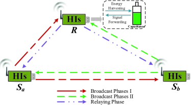
Figure 1: Model for the SWIPT based two-way DF relay network under a TDBC protocol.

II System Model and Working Flow

II-A System Model and Channel Model

We consider a SWIPT based two-way DF relay network under a TDBC protocol, where terminal $S_{a}$ communicates with terminal $S_{b}$ with the aid of an energy-limited relay $R$, as shown in Fig. 1. Herein, $R$ harvests energy from the incident RF signal following a PS scheme and a harvest-then-forward protocol. We assume that all nodes are equipped with a single antenna and operate in the half-duplex mode.

In the TDBC protocol, each transmission block $T$ is split into three phases, viz., two broadcast (BC) phases (each of duration $T/3$) and one relaying (RL) phase ($T/3$). During the first BC phase, $S_{a}$ transmits its signal $x_{a}$ to $R$ and $S_{b}$. In the second BC phase, $S_{b}$ broadcasts its signal $x_{b}$ to $R$ and $S_{a}$. After receiving the signal from $S_{a}$ or $S_{b}$, $R$ splits it into two parts, i.e., one part is for energy harvesting (EH) and the other is for information decoding (ID). During the RL phase, $R$ combines the decoded signals $x_{a}$ and $x_{b}$ using the bit-wise XOR based encoding [21], and then broadcasts the combined signal to $S_{a}$ and $S_{b}$ using the total harvested energy.

We assume that all channels are quasi-static and reciprocal, and subject to i.n.i.d. Nakagami-$m$ fading. Specifically, $h_{ij}\sim{\rm{Naka}}(m_{d},\Omega_{d})$ and $h_{ir}\sim{\rm{Naka}}(m_{i},\Omega_{i})$ represent the channel fading coefficients of the $S_{i}\rightarrow S_{j}$ and $S_{i}\rightarrow R$ links, respectively, with $i,j\in\left\{{a,b}\right\},\;i\neq j$. Since $h_{ij}$ and $h_{ir}$ follow the Nakagami distribution, the corresponding channel gains $|{h_{ij}}{|^{2}}$ and $|{h_{ir}}{|^{2}}$ follow independent and non-identical gamma distributions, and their PDF and CDF are expressed as

$${f_{V}}\left(v\right)=\frac{1}{{\Gamma\left({{m}}\right)\theta^{{m}}}}{v^{{m}-1}}{e^{-\frac{v}{{{\theta}}}}},$$ (1)

$${F_{V}}\left(v\right)=\frac{1}{{\Gamma\left({{m}}\right)}}\gamma\left({{m},\;\frac{v}{{{\theta}}}}\right),$$ (2)

where $m$ and $\theta$ denote the shape parameter³ and the scale parameter of random variable $V$, respectively, $V\in\left\{{|{h_{ij}}{|^{2}},|{h_{ir}}{|^{2}}}\right\}$, $i,j\in\{{a,b}\},i\neq j$. Specially, when $V{\rm{=}}|{h_{ij}}{|^{2}}$ or ${|{h_{ir}}{|^{2}}}$, $m={m_{d}}$ or ${{m_{i}}}$, and $\theta{\rm{=}}{\Omega_{d}}/{m_{d}}$ or ${{\Omega_{i}}/{m_{i}}}$, respectively.

II-B Working Flow

As mentioned above, $S_{a}$ and $S_{b}$ broadcast the signals $x_{a}$ and $x_{b}$ in the first second BC phases respectively.

For the direct link $\left({S_{i}}\mathop{\to}{S_{j}},i,j\in\left\{{a,b}\right\},i\neq j\right)$, as illustrated in Fig. 2 at the top of the next page, the received signal at $S_{j}$ from $S_{i}$, in the presence of HIs, can be expressed as [21]

$${y_{ij}}={h_{ij}}\left({{x_{i}}+{\tau_{t,i}}}\right)+{\tau_{r,j}}+{n_{ij}},$$ (3)

where ${x_{i}}$ is the signal transmitted by $S_{i}$ with ${P_{i}}={\mathbb{E}}\left\{{{{\left|{{x_{i}}}\right|}^{2}}}\right\}$, ${\tau_{t,i}}\sim\mathcal{CN}\left({0,k_{1}^{2}{P_{i}}}\right)$ represents the distortion noise generated by the transmitter of $S_{i}$⁴, ${\tau_{r,j}}\sim\mathcal{CN}\left({0,k_{2}^{2}{P_{i}}|{h_{ij}}{|^{2}}}\right)$ represents the distortion noise generated by the receiver of $S_{j}$ and ${{n_{ij}}}\sim\mathcal{CN}\left({0,\sigma^{2}}\right)$ is the additive white Gaussian noise (AWGN) at $S_{j}$. Note that $k_{1}$ and $k_{2}$ characterize the HIs levels of the transmitter and receiver, respectively, and are assumed to be the same for each transceiver [16]. For simplicity, we assume that $P_{a}=P_{b}=P_{o}$ [12].

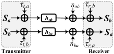
Figure 2: The signal flow diagram of the direct link under HIs.

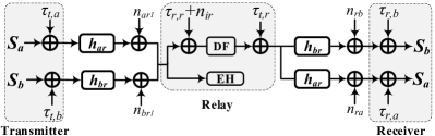
Figure 3: The signal flow diagram of the relaying link under HIs.

Based on (3), the signal-to-noise-plus-distortion ratio (SNDR) at $S_{j}$ from the direct link is written as

$${\gamma_{ij}}=\frac{{{\rho}|{h_{ij}}{|^{2}}}}{{\left({k_{1}^{2}+k_{2}^{2}}\right){\rho}|{h_{ij}}{|^{2}}+1}},$$ (4)

where $\rho=\frac{{{P_{o}}}}{{{\sigma^{2}}}}$ denotes the input signal-to-noise ratio (SNR).

For the relaying link $\left({S_{i}}\mathop{\to}\limits^{R}{S_{j}},i,j\in\left\{{a,b}\right\},i\neq j\right)$, as presented in Fig. 3, the received signal from $S_{i}$ at $R$, in the presence of HIs, can be written as

$${y_{ir}}={h_{ir}}\left({{x_{i}}+{\tau_{t,i}}}\right)+{n_{i{r_{1}}}},$$ (5)

where ${\tau_{t,i}}\sim\mathcal{CN}\left({0,k_{1}^{2}{P_{o}}}\right)$ represents the hardware distortion noise generated by the transmitter of $S_{i}$ and ${n_{ir_{1}}}\sim\mathcal{CN}\left({0,\sigma_{ir_{1}}^{2}}\right)$ is the antenna noise at $R$.

Using the PS protocol, the received signal ${y_{ir}}$ is split into two parts via a PS ratio $\beta$ ($0<\beta<1$): $\sqrt{\beta}{y_{ir}}$ for EH and $\sqrt{1-\beta}{y_{ir}}$ for ID. Thus, all the harvested energy during the two BC phases can be expressed as [21]

$${E_{h}}=\frac{T}{3}\eta\beta{P_{o}}\left({|{h_{ar}}{|^{2}}+|{h_{br}}{|^{2}}}\right),$$ (6)

where $\eta\in(0,1)$ denotes the energy conversion efficiency. Based on (6), the transmit power at $R$ can be calculated as

$${P_{r}}=\frac{{{E_{h}}}}{{T/3}}=\eta\beta{P_{o}}\left({|{h_{ar}}{|^{2}}+|{h_{br}}{|^{2}}}\right).$$ (7)

Furthermore, at the relay $R$, the received signal from $S_{i}$ used for ID can be written as

$$y_{ir}^{{\rm{ID}}}={h_{ir}}\sqrt{1-\beta}\left({{x_{i}}+{\tau_{t,i}}}\right)+{\tau_{r,r}}+{n_{ir}},$$ (8)

where ${\tau_{r,r}}\sim\mathcal{CN}\left({0,k_{2}^{2}(1-\beta){P_{o}}{|{h_{ir}}{|^{2}}}}\right)$ represents the distortion noise⁵ generated by the receiver of $R$ and ${n_{ir}}\sim\mathcal{CN}\left({0,\sigma^{2}}\right)$ is the AWGN at $R$.

Based on (8), the SNDR for decoding $x_{i}$ at $R$ is given by

$${\gamma_{ir}}=\frac{{\left({1-\beta}\right)\rho{{\left|{{h_{ir}}}\right|}^{2}}}}{{\left({k_{1}^{2}+k_{2}^{2}}\right)\left({1-\beta}\right)\rho{{\left|{{h_{ir}}}\right|}^{2}}+1}}.$$ (9)

If both $x_{a}$ and $x_{b}$ are successfully decoded during the two BC phases, $R$ performs bit-wise XOR based encoding to obtain the re-encoded signal $x_{r}$, i.e., ${x_{r}}={x_{a}}\oplus{x_{b}}$ with ${P_{r}}={\mathbb{E}}\left\{{{{\left|{{x_{r}}}\right|}^{2}}}\right\}$ [21]. Then $R$ broadcasts the signal $x_{r}$ to both terminals in the RL phase. Accordingly, the received signal at $S_{i}$ from $R$ can be written as

$${y_{ri}}={h_{ri}}\left({{x_{r}}+{\tau_{t,r}}}\right){\rm{+}}{\tau_{r,i}}+{n_{ri}},$$ (10)

where ${\tau_{t,r}}\sim\mathcal{CN}\left({0,k_{1}^{2}P_{r}}\right)$ represents the distortion noise generated by the transmitter of $R$, ${\tau_{r,i}}\sim\mathcal{CN}\left({0,k_{2}^{2}{P_{r}}{|{h_{ri}}{|^{2}}}}\right)$ represents the distortion noise generated by the receiver of $S_{i}$ and ${n_{ri}}\sim\mathcal{CN}\left({0,\sigma^{2}}\right)$ is the AWGN at $S_{i}$.

$${\mathbb{P}_{{{out}}}}=\underbrace{\Pr\left\{{\left({1-\left({k_{1}^{2}+k_{2}^{2}}\right){\gamma_{th}}}\right)\rho Z<{\gamma_{th}}}\right\}}_{{\mathbb{P}_{1}}}\!\!\left(\!{1\!-\!\underbrace{\Pr\left\{\begin{array}[]{l}\left({1-\beta}\right)\left({1\!-\!\left({k_{1}^{2}\!+\!k_{2}^{2}}\right){\gamma_{th}}}\right)\rho X\!>\!{\gamma_{th}},\\ \left({1-\beta}\right)\left({1\!-\!\left({k_{1}^{2}\!+\!k_{2}^{2}}\right){\gamma_{th}}}\right)\rho Y\!>\!{\gamma_{th}},\\ \eta\beta\left({1\!-\!\left({k_{1}^{2}\!+\!k_{2}^{2}}\right){\gamma_{th}}}\right)\rho X\left({X+Y}\right)\!>\!{\gamma_{th}},\\ \eta\beta\left({1\!-\!\left({k_{1}^{2}\!+\!k_{2}^{2}}\right){\gamma_{th}}}\right)\rho Y\left({X+Y}\right)\!>\!{\gamma_{th}}\end{array}\right\}}_{{\mathbb{P}_{2}}}}\!\right)$$ (18)

$$\mathbb{P}_{2}^{1}=\frac{1}{{\Gamma\left({{m_{a}}}\right)}}\Gamma\left({{m_{a}},{\Delta_{1}}/{\theta_{a}}}\right)-\frac{1}{{\Gamma\left({{m_{a}}}\right)\theta_{a}^{{m_{a}}}}}\sum\limits_{l=0}^{{m_{b}}-1}{\frac{1}{{l!}}}{\left({\frac{1}{{{\theta_{b}}}}}\right)^{l}}{\left({\frac{1}{{{\theta_{a}}}}+\frac{1}{{{\theta_{b}}}}}\right)^{-\left({l+{m_{a}}}\right)}}\Gamma\left({l+{m_{a}},{\Delta_{1}}\left({\frac{1}{{{\theta_{a}}}}+\frac{1}{{{\theta_{b}}}}}\right)}\right)$$

$$+\frac{1}{{\Gamma\left({{m_{b}}}\right)}}\Gamma\left({{m_{b}},{\Delta_{1}}/{\theta_{b}}}\right)-\frac{1}{{\Gamma\left({{m_{b}}}\right)\theta_{b}^{{m_{b}}}}}\sum\limits_{l=0}^{{m_{a}}-1}{\frac{1}{{l!}}}{\left({\frac{1}{{{\theta_{a}}}}}\right)^{l}}{\left({\frac{1}{{{\theta_{a}}}}+\frac{1}{{{\theta_{b}}}}}\right)^{-\left({l+{m_{b}}}\right)}}\Gamma\left({l+{m_{b}},{\Delta_{1}}\left({\frac{1}{{{\theta_{a}}}}+\frac{1}{{{\theta_{b}}}}}\right)}\right)$$

$$\!-\!\frac{1}{{\Gamma\left(\!{{m_{b}}}\!\right)}}\gamma\left(\!{{m_{b}},\!{\Delta_{1}}/{\theta_{b}}}\!\right)\!\left(\!{1\!-\!\frac{1}{{\Gamma\left({{m_{a}}}\right)}}\gamma\left({{m_{a}},{\Delta_{1}}/{\theta_{a}}}\right)}\right)\!-\!\frac{1}{{\Gamma\left(\!{{m_{a}}}\right)}}\gamma\left({{m_{a}},{\Delta_{1}}/{\theta_{a}}}\right)\left({1\!-\!\frac{1}{{\Gamma\left({{m_{b}}}\right)}}\gamma\left({{m_{b}},{\Delta_{1}}/{\theta_{b}}}\right)}\right)$$ (18)

According to (10), the SNDR at $S_{i}$ from the relay link can be expressed as

$${\gamma_{ri}}=\frac{{\eta\beta\rho{{\left|{{h_{ir}}}\right|}^{2}}\left(\!{{{\left|{{h_{ar}}}\right|}^{2}}\!+\!{{\left|{{h_{br}}}\right|}^{2}}}\!\right)}}{{\left({k_{1}^{2}\!+\!k_{2}^{2}}\right)\eta\beta\rho{{\left|{{h_{ir}}}\right|}^{2}}\left({{{\left|{{h_{ar}}}\right|}^{2}}\!+\!{{\left|{{h_{br}}}\right|}^{2}}}\right)\!+\!1}}.$$ (11)

Following the selection combining scheme, the end-to-end SNDR at $S_{i}$ can be written as

$${\gamma_{i}}=\max\left\{{{\gamma_{ji}},\min\left\{{{\gamma_{jr}},{\gamma_{ri}}}\right\}}\right\},$$ (12)

where $i,j\in\left\{{a,b}\right\},i\neq j$.

III System Outage Performance Analysis

In this section, we first derive the system outage probability in closed-form, then identify the OSC effect, and study the achievable diversity gain of our studied network.

III-A System Outage Probability

The outage event occurs if the data rate $\mathbf{R}_{a}$ from $S_{a}$ to $S_{b}$ and/or the data rate $\mathbf{R}_{b}$ from $S_{b}$ to $S_{a}$ falls below a threshold $\mathbf{R}_{th}$ [6]. Hence, the system outage probability⁶, $\mathbb{P}_{out}$, can be written as

$${\mathbb{P}_{out}}=\Pr\left\{{\min\left\{{{{\mathbf{R}}_{a}},{{\mathbf{R}}_{b}}}\right\}<{{\mathbf{R}}_{th}}}\right\}$$

$$=\Pr\left\{{\min\left\{{{\gamma_{a}},{\gamma_{b}}}\right\}<{\gamma_{th}}}\right\}=\Pr\left\{{{\gamma_{ab}}<{\gamma_{th}}}\right\}$$

$$\!\times\!\left(\!{1\!-\!\Pr\left\{\!{{\gamma_{ar}}\!>\!{\gamma_{th}},{\gamma_{br}}\!>\!{\gamma_{th}},{\gamma_{ra}}\!>\!{\gamma_{th}},{\gamma_{rb}}\!>\!{\gamma_{th}}}\!\right\}}\!\right),$$ (13)

where ${\gamma_{th}}={2^{{{3{{\mathbf{R}}_{{{th}}}}}\mathord{\left/{\vphantom{{3{{\mathbb{R}}_{{{th}}}}}T}}\right.\kern-1.2pt}T}}}-1$ denotes the SNDR threshold and ${\mathbf{R}}_{i}=\frac{T}{3}{\log_{2}}\left({1+{\gamma_{i}}}\right)$, $i\in\{a,b\}$.

Letting $|{h_{ar}}{|^{2}}=X$, $|{h_{br}}{|^{2}}=Y$ and $|{h_{ab}}{|^{2}}=Z$, and substituting (4), (9) and (11) into (III-A), ${\mathbb{P}_{out}}$ can be rewritten as (18).

$$\mathbb{P}_{2}^{2}=\frac{{\pi\left({\Phi-\sqrt{{\Delta_{2}}/2}}\right)}}{{2N\Gamma\left({{m_{a}}}\right)\theta_{a}^{{m_{a}}}}}\sum\limits_{l=0}^{{m_{b}}-1}{\sum\limits_{n=1}^{N}{\sqrt{1-v_{n}^{2}}\frac{1}{{l!}}{{\left({\frac{1}{{{\theta_{b}}}}}\right)}^{l}}}}{\left({k_{n}^{{}^{\prime}}+\sqrt{{\Delta_{2}}/2}}\right)^{{m_{a}}-1}}{Q^{l}}\left({k_{n}^{{}^{\prime}}+\sqrt{{\Delta_{2}}/2}}\right)$$

$$\times{e^{-\frac{{k_{n}^{{}^{\prime}}+\sqrt{{\Delta_{2}}/2}}}{{{\theta_{a}}}}-\frac{{Q\left({k_{n}^{{}^{\prime}}+\sqrt{{\Delta_{2}}/2}}\right)}}{{{\theta_{b}}}}}}-\frac{1}{{\Gamma\left({{m_{a}}}\right)\theta_{a}^{{m_{a}}}}}\sum\limits_{l=0}^{{m_{b}}-1}{\frac{1}{{l!}}}{\left({\frac{1}{{{\theta_{b}}}}}\right)^{l}}{\left({\frac{{{\theta_{a}}{\theta_{b}}}}{{{\theta_{a}}+{\theta_{b}}}}}\right)^{{m_{a}}+l}}\bigg{(}\gamma\left({{m_{a}}+l,\Phi\left({\frac{1}{{{\theta_{a}}}}+\frac{1}{{{\theta_{b}}}}}\right)}\right)$$

$$-\gamma\left({{m_{a}}+l,\sqrt{{\Delta_{2}}/2}\left({\frac{1}{{{\theta_{a}}}}+\frac{1}{{{\theta_{b}}}}}\right)}\right)\bigg{)}+\frac{{\pi\left({\Phi-\sqrt{{\Delta_{2}}/2}}\right)}}{{2N\Gamma\left({{m_{b}}}\right)\theta_{b}^{{m_{b}}}}}\sum\limits_{l=0}^{{m_{a}}-1}{\sum\limits_{n=1}^{N}{\sqrt{1-v_{n}^{2}}\frac{1}{{l!}}{{\left({\frac{1}{{{\theta_{a}}}}}\right)}^{l}}}}{\left({k_{n}^{\rm{{}^{\prime}}}+\sqrt{{\Delta_{2}}/2}}\right)^{{m_{b}}-1}}$$

$$\times{Q^{l}}\left({k_{n}^{{{}^{\prime}}}+\sqrt{{\Delta_{2}}/2}}\right){e^{-\frac{{k_{n}^{{{}^{\prime}}}+\sqrt{{\Delta_{2}}/2}}}{{{\theta_{b}}}}-\frac{{Q\left({k_{n}^{{{}^{\prime}}}+\sqrt{{\Delta_{2}}/2}}\right)}}{{{\theta_{a}}}}}}-\frac{1}{{\Gamma\left({{m_{b}}}\right)\theta_{b}^{{m_{b}}}}}\sum\limits_{l=0}^{{m_{a}}-1}{\frac{1}{{l!}}}{\left({\frac{1}{{{\theta_{a}}}}}\right)^{l}}{\left({\frac{{{\theta_{a}}{\theta_{b}}}}{{{\theta_{a}}+{\theta_{b}}}}}\right)^{{m_{b}}+l}}$$

$$\times\left({\gamma\left({{m_{b}}+l,\Phi\left({\frac{1}{{{\theta_{a}}}}+\frac{1}{{{\theta_{b}}}}}\right)}\right)-\gamma\left({{m_{b}}+l,\sqrt{{\Delta_{2}}/2}\left({\frac{1}{{{\theta_{a}}}}+\frac{1}{{{\theta_{b}}}}}\right)}\right)}\right)$$

$$+\frac{1}{{\Gamma\left({{m_{a}}}\right)}}\Gamma\left({{m_{a}},\Phi/{\theta_{a}}}\right)-\frac{1}{{\Gamma\left({{m_{a}}}\right)\theta_{a}^{{m_{a}}}}}\sum\limits_{l=0}^{{m_{b}}-1}{\frac{1}{{l!}}}{\left({\frac{1}{{{\theta_{b}}}}}\right)^{l}}{\left({\frac{1}{{{\theta_{a}}}}+\frac{1}{{{\theta_{b}}}}}\right)^{-\left({l+{m_{a}}}\right)}}\Gamma\left({l+{m_{a}},\Phi\left({\frac{1}{{{\theta_{a}}}}+\frac{1}{{{\theta_{b}}}}}\right)}\right)$$

$$+\frac{1}{{\Gamma\left({{m_{b}}}\right)}}\Gamma\left({{m_{b}},\Phi/{\theta_{b}}}\right)-\frac{1}{{\Gamma\left({{m_{b}}}\right)\theta_{b}^{{m_{b}}}}}\sum\limits_{l=0}^{{m_{a}}-1}{\frac{1}{{l!}}}{\left({\frac{1}{{{\theta_{a}}}}}\right)^{l}}{\left({\frac{1}{{{\theta_{a}}}}+\frac{1}{{{\theta_{b}}}}}\right)^{-\left({l+{m_{b}}}\right)}}\Gamma\left({l+{m_{b}},\Phi\left({\frac{1}{{{\theta_{a}}}}+\frac{1}{{{\theta_{b}}}}}\right)}\right)$$

$$\!-\!\frac{1}{{\Gamma\left({{m_{b}}}\right)}}\gamma\left({{m_{b}},{\Delta_{1}}/{\theta_{b}}}\right)\!\left({1\!-\!\frac{1}{{\Gamma\left({{m_{a}}}\right)}}\gamma\left({{m_{a}},\!\Phi/{\theta_{a}}}\right)}\right)\!-\!\frac{1}{{\Gamma\left({{m_{a}}}\right)}}\gamma\left({{m_{a}},{\Delta_{1}}/{\theta_{a}}}\right)\left({1\!-\!\frac{1}{{\Gamma\left({{m_{b}}}\right)}}\gamma\left({{m_{b}},\Phi/{\theta_{b}}}\right)}\right)$$ (19)

Next, we derive $\mathbb{P}_{1}$ and $\mathbb{P}_{2}$ to obtain the closed-form expression for $\mathbb{P}_{out}$ respectively. The first term of (18), $\mathbb{P}_{1}$, can be calculated as

$${\mathbb{P}_{1}}=\left\{\begin{array}[]{l}{\mathbb{P}_{1}^{1}}\;,\;\;{\gamma_{th}}<\frac{1}{{k_{1}^{2}+k_{2}^{2}}},\\ \;1\;\;,\;\;{\gamma_{th}}\geq\frac{1}{{k_{1}^{2}+k_{2}^{2}}},\end{array}\right.$$ (17)

where ${\mathbb{P}_{1}^{1}}$ is given by

$${\mathbb{P}_{1}^{1}}= 1-{e^{-\frac{{{\gamma_{th}}}}{{{\theta_{d}}\rho\left({1-{\gamma_{th}}\left({k_{1}^{2}+k_{2}^{2}}\right)}\right)}}}}$$

$$\times\sum\limits_{l=0}^{{m_{d}}-1}{\frac{1}{{l!}}}{\left({\frac{{{\gamma_{th}}}}{{{\theta_{d}}\rho\left({1-{\gamma_{th}}\left({k_{1}^{2}+k_{2}^{2}}\right)}\right)}}}\right)^{l}}.$$ (18)

Proof. Please refer to Appendix A. $\blacksquare$

The second term of (18), $\mathbb{P}_{2}$, can be calculated as

$${\mathbb{P}_{2}}=\left\{\begin{array}[]{l}{\mathbb{P}_{2}^{*}}\;,\;\;{\gamma_{th}}<\frac{1}{{k_{1}^{2}+k_{2}^{2}}},\\ \;0\;\;,\;\;{\gamma_{th}}\geq\frac{1}{{k_{1}^{2}+k_{2}^{2}}},\end{array}\right.$$ (19)

where ${\mathbb{P}_{2}^{*}}$ equals either ${\mathbb{P}_{2}^{1}}$ or ${\mathbb{P}_{2}^{2}}$, as presented respectively in (II-B) at the top of the previous page and (III-A). Please note that, ${\mathbb{P}_{2}^{1}}$ corresponds to the case that ${\Delta_{\rm{1}}}\geq\sqrt{{\Delta_{\rm{2}}}{\rm{/2}}}$ is satisfied (as discussed in Appendix B), while ${\mathbb{P}_{2}^{2}}$ corresponds to the case that ${\Delta_{\rm{1}}}<\sqrt{{\Delta_{\rm{2}}}{\rm{/2}}}$ holds, where ${\Delta_{1}}=\frac{{{\gamma_{th}}}}{{\left({1-\beta}\right)\left({1-\left({k_{1}^{2}+k_{2}^{2}}\right){\gamma_{th}}}\right)\rho}}$ and ${\Delta_{2}}=\frac{{{\gamma_{th}}}}{{\eta\beta\left({1-\left({k_{1}^{2}+k_{2}^{2}}\right){\gamma_{th}}}\right)\rho}}$.

Proof. Please refer to Appendix B. $\blacksquare$

Substituting (17) and (19) into (18), the system outage probability of the considered network can be expressed as

$${\mathbb{P}_{out}}=\left\{\begin{array}[]{l}{\mathbb{P}_{1}^{1}}\left(1-{\mathbb{P}_{2}^{*}}\right)\;,\;\;{\gamma_{th}}<\frac{1}{{k_{1}^{2}+k_{2}^{2}}},\\ \;\;\;\;\;\;\;\;\;1\;\;\;\;\;\;\;\;,\;\;{\gamma_{th}}\geq\frac{1}{{k_{1}^{2}+k_{2}^{2}}}.\end{array}\right.$$ (22)

Remark 1

As illustrated in (22), HIs deteriorate the system outage performance by imposing a constraint on $\gamma_{th}$. In particular, when ${\gamma_{th}}<\frac{1}{{k_{1}^{2}+k_{2}^{2}}}$, both the direct and relaying links participate in the information exchange between two terminals. However, when ${\gamma_{th}}\geq\frac{1}{{k_{1}^{2}+k_{2}^{2}}}$, the overall system ceases no matter what the input SNR is. This effect is referred to as OSC, and $\frac{1}{{k_{1}^{2}+k_{2}^{2}}}$ denotes the corresponding OSC threshold. This ceiling effect is due to the fact that the instantaneous SNDRs at $S_{a}$, $S_{b}$ and $R$, given in (4), (9) and (11), are upper bounded by ${\gamma_{ij}}$, ${\gamma_{ir}}$, ${\gamma_{rj}}<\frac{1}{{k_{1}^{2}+k_{2}^{2}}}$, respectively, $i,j\in\{a,b\}$ and $i\neq j$. In addition, it is obvious that the maximum achievable SNDR threshold $\gamma^{max}_{th}\approx\frac{1}{{k_{1}^{2}+k_{2}^{2}}}$ decreases with the increase of the HIs levels.

III-B Diversity Gain

Referring to [23], the achievable diversity gain of the considered network can be given as

$$d=-\mathop{\lim}\limits_{\rho\to\infty}\frac{{\log\left({{\mathbb{P}_{out}}}\right)}}{{\log\left(\rho\right)}}.$$ (21)

Substituting (22) into (21), the diversity gain can be calculated as

$$d=\left\{\begin{array}[]{l}m_{d}+\min\left({{m_{a}},{m_{b}}}\right)\;\;,\;{\gamma_{th}}<\frac{1}{{k_{1}^{2}+k_{2}^{2}}},\\ \;\;\;\;\;\;\;\;\;\;\;\;\;\;0\;\;\;\;\;\;\;\;\;\;\;\;\;\;\;\;\;,\;{\gamma_{th}}\geq\frac{1}{{k_{1}^{2}+k_{2}^{2}}}.\end{array}\right.$$ (24)

Proof. Please refer to Appendix C. $\blacksquare$

Remark 2

Eq. (24) reveals the following facts. When ${\gamma_{th}}$ exceeds the OSC threshold, vie., ${\gamma_{th}}\geq\frac{1}{{k_{1}^{2}+k_{2}^{2}}}$, the diversity gain of the overall system is equal to zero. When ${\gamma_{th}}<\frac{1}{{k_{1}^{2}+k_{2}^{2}}}$, the diversity gain is the sum of the shape parameter of the direct link and the smaller shape parameter of the terminal-to-relay links. In other words, both the direct and relaying links jointly enhance the diversity gain. However, for the AF strategy, HIs makes the diversity gain from the relaying links zero [22]. The reason is as follows. For the AF strategy, one observation from [20, eq. (10)] is that the SNDR of the relaying link at high $\rho$ is a function of channel fading coefficients, which cannot ensure that the SNDR is larger than its threshold with probability one even though $\rho\to\infty$. Accordingly, the achievable diversity gain of AF relaying links equals zero. Such a result is mainly due to the fact that the AF strategy amplifies the signals and distortion noises simultaneously. However, in the DF relaying, the SNDRs of both the relay and terminals at high $\rho$ keep constant, i.e., ${\gamma_{ir}}={\gamma_{rj}}=\frac{1}{{k_{1}^{2}+k_{2}^{2}}}$. When ${\gamma_{th}}<\frac{1}{{k_{1}^{2}+k_{2}^{2}}}$, the outage probability for the relaying links approaches zero with the increase of $\rho$, which allows the relaying links to contribute to the diversity gain.

IV Simulation Results

In this section, numerical results are provided to validate the correctness of the above theoretical analyses. Hereinafter, unless otherwise specified, the simulation parameters are set as Table 2 [21, 22, 24].

TABLE II: Simulation parameters

Parameter	Value
energy conversion efficiency, $\eta$	0.6
PS ratio, $\beta$	0.9
transmission block, $T$	1 s
HIs levels, $k_{1}$ and $k_{2}$	$k_{ave}$
the distances of $S_{a}-R$ link, $d_{ar}$	5 m
the distances of $S_{b}-R$ link, $d_{br}$	5 m
the distances of $S_{a}-S_{b}$ link, $d_{ab}$	10 m
the path loss exponents of the	2.7
relaying links, $\alpha_{1}$
the path loss exponents of the	3
direct link, $\alpha_{2}$
the average power, $\Omega_{a}$	$d_{ar}^{-{\alpha_{1}}}$
the average power, $\Omega_{b}$	$d_{br}^{-{\alpha_{1}}}$
the average power, ${\Omega_{d}}$	$d_{ab}^{-{\alpha_{2}}}$
the noise power $\sigma^{2}$	-50 dBm
the channel bandwidth	1 MHz

Fig. 4 verifies the derived system outage probability in all two cases of the (22). Based on the used simulation parameters, we determine the specific value for the OSC threshold, viz., $\frac{1}{{k_{1}^{2}+k_{2}^{2}}}=50$. In addition, we also consider four different transmission rates i.e., $\mathbb{R}_{th}=1$, $1.5$, $2$ and $2.5$ bit/Hz. On the basis of the definition in (III-A), the corresponding SNDR thresholds are calculated as $7$, $22$, $63$, and $180$ respectively. According to (22), when the SNDR threshold $\gamma_{th}=7\&22$ or $63\&180$, the corresponding system outage probability is expressed as ${\mathbb{P}_{1}^{1}}\left(1-{\mathbb{P}_{2}^{*}}\right)$ or $1$. As presented in Fig. 4, the ‘$\lozenge$, $\Box$, $\triangledown$, $\circ$’ marked curves (analytical results) match precisely with the ‘-’ marked curves (simulation results) across the entire region, which validates the correctness of the derived system outage probability in Section 3.1.

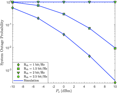
Figure 4: The derived system outage probability ${\mathbb{P}_{out}}$ vs. the transmit power of each terminal $P_{o}$, in comparison with simulation results, where $k_{ave}=0.1$ and $\{m_{a},m_{b},m_{d}\}=\{2,2,1\}$.

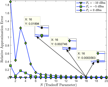
Figure 5: The relative approximation error vs. the trade-off parameter $N$, where $k_{ave}=0.1$, $\mathbb{R}_{th}=1$ bit/Hz and $\{m_{a},m_{b},m_{d}\}=\{2,2,1\}$.

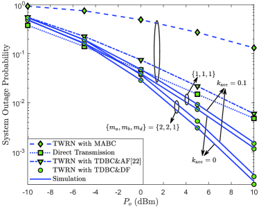
Figure 6: The system outage probability ${\mathbb{P}_{out}}$ vs. the transmit power of each terminal $P_{o}$, where $\mathbb{R}_{th}=1$ bit/Hz.

In Appendix B, the Gaussian-Chebyshev quadrature approach is adopted to obtain the approximate system outage probability ${\mathbb{P}_{2}^{2}}$ in (22) when ${\Delta_{\rm{1}}}<\sqrt{{\Delta_{\rm{2}}}{\rm{/2}}}$. To illustrate the performance of the Gaussian-Chebyshev quadrature approximation approach, Fig. 5 shows the relative approximation error against the tradeoff parameter $N$ for different transmit power of each terminal. Specially, the relative approximation error $\delta$ equals the ratio of the absolute value of difference between the simulation and analytical results to the simulation result, in which the simulation and analytical results are obtained by compute simulation and (22) respectively. From Fig. 5, one can observe that $\delta$ gradually approaches zero as $N$ increases. For instance, when $P_{o}\;=\;-5$ dBm and $N=16$, the corresponding $\delta$ is $0.002746$, which demonstrates that the Gaussian-Chebyshev quadrature with few terms can evaluate the system outage performance precisely.

Fig. 6 presents the system outage probability versus transmit power of each terminal $P_{o}$ for four transmission protocols, viz., the TDBC with DF strategy (viz., the considered network), the TDBC with AF strategy [22], the direct transmission, and the MABC. Herein, we ensure that the used target transmission rate satisfies ${\gamma_{th}}<\frac{1}{{k_{1}^{2}+k_{2}^{2}}}$. As given in Fig. 6, the considered network achieves the higher system outage performance than both the MABC and the direct transmission. One can also note that the system outage performance of the considered network outperforms that of the TDBC with AF strategy. This suggests that under the presence of HIs, the DF strategy is superior to AF strategy in terms of system outage performance. Additionally, it can be observed that, for the given shape parameters, the considered network exists a performance gap between the curves corresponding to ideal hardware ($k_{ave}=0$) and HIs ($k_{ave}=0.1$), which concludes that the HIs degrade the system outage performance to some extent. Finally, as expected, better channel quality of the relaying links can significantly improve the system outage performance for the considered network under a fixed HIs level.

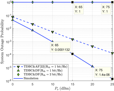
Figure 7: The derived diversity gain $d$ vs. the transmit power of each terminal $P_{o}$, in comparison with simulation results, where $k_{ave}=0.1$ and $\{m_{a},m_{b},m_{d}\}=\{2,1,1\}$.

Fig. 7 verifies the derived diversity gains in all two cases of the (24). Given two points ($x_{1}$, $y_{1}$) and ($x_{2}$, $y_{2}$) in the “$\bigtriangleup$”or “$\diamond$”marked curve in Fig. 7, we can calculate the slope of the curve as -2 or 0 by $\frac{{\log\left({{y_{1}}}\right)-\log\left({{y_{2}}}\right)}}{{\log\left({{{10}^{{x_{1}}/10}}}\right)-\log\left({{{10}^{{x_{2}}/10}}}\right)}}$, which is consistent with the derived diversity gain in Section 3.2. Additionally, as presented in this figure, when the target transmission rate is below the OSC threshold, both the direct and relaying links of the considered network jointly contribute to the diversity gain. However, the achievable diversity gain of the TDBC with AF strategy is only determined by the direct link. This is due to the relay node using AF strategy amplifies the distortion noises caused HIs, which in turn results in that the relaying links have no contribution to the diversity gain.

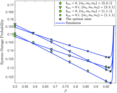
Figure 8: The system outage probability ${\mathbb{P}_{out}}$ vs. the PS ratio $\beta$, where $\mathbb{R}_{th}=1$ bit/Hz.

Fig. 8 depicts the system outage probability versus the PS ratio $\beta$. As presented in this figure, when $\beta$ increases, all curves decrease first and then increases. Such variation trend is owing to the following fact. According to (6), the harvested energy at $R$ gradually increases as $\beta$ increases. Meanwhile, the increase of $\beta$ also reduces the portion of the received signal used for ID at $R$. When $\beta$ increases from zero to the optimal value, the increase of the transmit power at $R$ dominantly enhance the system outage performance. However, when $\beta$ exceeds the optimal value and further increases, it is hard for $R$ to decode information from two terminals, which in turn increases the system outage probability. Additionally, it can be observed that, for the fixed $k_{ave}$, the optimal $\beta$ increases as shape parameters of the relaying links increase. This is because $R$ needs fewer portion of the received signal used for ID as the channel quality of the relaying links improves.

Figure 9: The system outage probability ${\mathbb{P}_{out}}$ vs. the SNDR threshold $\gamma_{th}$, where $P_{o}=10$ dBm and $\{m_{a},m_{b},m_{d}\}=\{2,2,1\}$.

Fig. 9 shows the system outage probability as a function of the SNDR threshold $\gamma_{th}$ using either HIs ($k_{ave}=0.15$) or ideal hardware ($k_{ave}=0$) assumption. From this figure, it can be observed that when $\gamma_{th}$ is below $22.2$, i.e., the OSC threshold $\frac{1}{{k_{1}^{2}+k_{2}^{2}}}$, the system outage performance of our studied network under HIs relies on both the direct and relaying links. Nevertheless, when $\gamma_{th}$ goes beyond the OSC threshold, the overall system ceases. These results coincide with the conclusions in Remark 1. Moreover, the impact of HIs is negligible for a low SNDR threshold, but it becomes very severe with increasing $\gamma_{th}$. Note that, different from the studied network, the SWIPT based AF TWRN suffers from not only the OSC effect but also the RCC effect. More specifically, the RCC prevents the relaying link from carrying out cooperative communication, while the OSC puts the overall system in outage. In addition, we also observe that the relaying links under the AF strategy are more sensitive to HIs than those under the DF strategy.

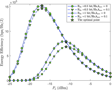
Figure 10: Energy efficiency vs. the transmit power of each terminal $P_{o}$, where $\{m_{a},m_{b},m_{d}\}=\{2,2,1\}$.

Fig. 10 studies the influence of transmit power of each terminal $P_{o}$ on the energy efficiency to get some insights about the utilization of the available energy. Specially, the energy efficiency is defined as $EE=\frac{{{\mathbb{R}_{th}}\left({1-{{\rm{\mathbb{P}}}_{out}}}\right)}}{{2T{P_{o}}/3}}$, where ${{\rm{\mathbb{P}}}_{out}}$ can be obtained from (22) [25]. From this figure, it can be observed that all curves exist the optimal $P_{o}$ maximizing the energy efficiency. In addition, we can also note that the achievable energy efficiency is low at high $P_{o}$ region. This is due to the achieved system outage performance is much lower than the consumed energy at high transmit power region. Furthermore, for a fixed transmission rate, the energy efficiency under practical case ($k_{ave}=0.1$) is much lower than that under ideal case ($k_{ave}=0$). This is because the HIs impose an undesirable influence on the system outage performance of our considered network.

V Conclusion

In this work, we have analyzed the system outage probability and the diversity gain of a SWIPT based two-way DF relaying, in which HIs at all transceivers are taken into account. In particular, under i.n.i.d. Nakagami-$m$ fading channels, the closed-form expression for the system outage probability has been obtained. Based the derived expression, we have identified the OSC effect and obtained the achievable diversity gain of our studied network. Our analytical results have revealed the following fact, i.e., when transmission rate goes beyond the OSC threshold, the overall system is in outage and the diversity gain is zero; otherwise, both the direct and relaying links contribute to enhancing the system outage performance and the resulting diversity gain is the sum of the shape parameter of the direct link and the smaller shape parameter of the terminal-to-relay links, viz., $d=m_{d}+\min\left({{m_{a}},{m_{b}}}\right)$. In addition, numerical results have provided some insights about the effect of multifarious parameters on system outage performance as well as the performance difference between DF and AF strategies. Based on the results, we have provided guideline on how terminals use energy to balance the energy utilization and spectral utilization.

Appendix A

In order to obtain the closed-form expression for $\mathbb{P}_{1}$, we divide into the following two cases in terms of the range of ${\gamma_{th}}$.

Case 1: When ${\gamma_{th}}\geq\frac{1}{{k_{1}^{2}+k_{2}^{2}}}$ holds, the inequality of $\mathbb{P}_{1}$, ${\left({1-\left({k_{1}^{2}+k_{2}^{2}}\right){\gamma_{th}}}\right)\rho Z<{\gamma_{th}}}$, is always true no matter what value random variable $Z$ $(Z>0)$ takes. Therefore, the corresponding probability equals one, viz., $\mathbb{P}_{1}=1$.

Case 2: When ${\gamma_{th}}<\frac{1}{{k_{1}^{2}+k_{2}^{2}}}$ is satisfies, $\mathbb{P}_{1}$ can be re-expressed as $\mathbb{P}_{1}^{1}$, given by

$${\mathbb{P}_{1}^{1}} =\Pr\left({Z<\frac{{{\gamma_{th}}}}{\rho{\left({1-{\gamma_{th}}\left({k_{1}^{2}+k_{2}^{2}}\right)}\right)}}}\right)$$

$$=\int_{0}^{\frac{{{\gamma_{th}}}}{\rho{\left({1-{\gamma_{th}}\left({k_{1}^{2}+k_{2}^{2}}\right)}\right)}}}{\frac{1}{{\Gamma\left({{m_{d}}}\right)\theta_{d}^{{m_{d}}}}}}{z^{{m_{d}}-1}}{e^{-\frac{z}{{{\theta_{d}}}}}}dz,$$ (A.1)

where $m_{d}$ and ${\theta_{d}}=\frac{{{\Omega_{d}}}}{{{m_{d}}}}$ are the shape and scale parameters of the gamma random variable $Z$ respectively. According to [29, eq.(3.381.1)] and [29, eq.(8.352.6)], we can solve the integration of (A), and then obtain the closed-form expression for ${\mathbb{P}_{1}^{1}}$ as given in (III-A).

Appendix B

Based on the above analysis of $\mathbb{P}_{1}$, we can also derive the closed-form expression for $\mathbb{P}_{2}$ in terms of the following two cases.

Case 1: When ${\gamma_{th}}\geq\frac{1}{{k_{1}^{2}+k_{2}^{2}}}$ is satisfied, all the inequalities of $\mathbb{P}_{2}$ are never true. Therefore, the corresponding probability is equal to zero, i.e., $\mathbb{P}_{2}=1$.

Case 2: When ${\gamma_{th}}<\frac{1}{{k_{1}^{2}+k_{2}^{2}}}$ holds, $\mathbb{P}_{2}$ can be rewritten as $\mathbb{P}_{2}=\Pr\{X>{\Delta_{1}},Y>{\Delta_{1}},X>-Y+{\Delta_{2}}/Y,Y>-X+{\Delta_{2}}/X\}$, where ${\Delta_{1}}=\frac{{{\gamma_{th}}}}{{\left({1-\beta}\right)\left({1-\left({k_{1}^{2}+k_{2}^{2}}\right){\gamma_{th}}}\right)\rho}}$ and ${\Delta_{2}}=\frac{{{\gamma_{th}}}}{{\eta\beta\left({1-\left({k_{1}^{2}+k_{2}^{2}}\right){\gamma_{th}}}\right)\rho}}$. Obviously, there is the high correlation among the inequalities in $\mathbb{P}_{2}$, which is the main obstacle in deriving $\mathbb{P}_{2}$. Assume that $X=x$ and $Y=y$. From the expression of $\mathbb{P}_{2}$ in (18), the integral region of $\mathbb{P}_{2}$ is bounded by four curves, which are ${l_{1}}:x={\Delta_{1}}$, ${l_{2}}:y={\Delta_{1}}$, ${l_{3}}:x=-y+{\Delta_{2}}/y$ and ${l_{4}}:y=-x+{\Delta_{2}}/x$. After straightforward mathematical manipulations for the above four curves, we can obtain several conclusions as follows:

1) curves $l_{3}(y)$ and $l_{4}(x)$ are the monotonically decreasing functions with respect of $y$ and $x$ respectively, where $x,y\in\left({0,+\infty}\right)$.

2) $\mathop{\lim}\limits_{x\to 0}\left({-x+{\Delta_{2}}/x}\right)=+\infty$ and $\mathop{\lim}\limits_{y\to 0}\left({-y+{\Delta_{2}}/y}\right)=+\infty$;

3) the zero point of curve $l_{3}$ ($l_{4}$) at y(x)-axis is $y=\sqrt{{\Delta_{2}}}$ $\left(x=\sqrt{{\Delta_{2}}}\right)$;

4) curves $l_{3}$ and $l_{4}$ are symmetric about $l_{5}:y=x$;

5) the intersection between curves $l_{3}$ and $l_{4}$ is $\left({\sqrt{{\Delta_{2}}/2},\sqrt{{\Delta_{2}}/2}}\right)$ in the first quadrant;

6) the intersection between curves $l_{3}$ ($l_{4}$) and $l_{5}$ is $\left({\sqrt{{\Delta_{2}}/2},\sqrt{{\Delta_{2}}/2}}\right)$ in the first quadrant;

Based on the above conclusions, there are two cases for the integral region of $\mathbb{P}_{2}$, discussed as follows.

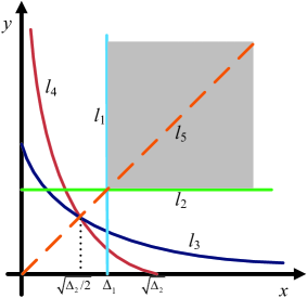
Figure 11: The integral region for $\mathbb{P}_{2}$, where ${\Delta_{\rm{1}}}\geq\sqrt{{\Delta_{\rm{2}}}{\rm{/2}}}$.

i): When ${\Delta_{\rm{1}}}\geq\sqrt{{\Delta_{\rm{2}}}{\rm{/2}}}$ holds, the integral region for $\mathbb{P}_{2}$ can be shown as the shadow area in Fig. 11. Thus, $\mathbb{P}_{2}$ can be expressed as ${\mathbb{P}_{2}^{1}}$, given by

$${\mathbb{P}_{2}^{1}}= \underbrace{\int_{{\Delta_{1}}}^{\infty}{\int_{{\Delta_{1}}}^{x}{{f_{Y}}\left(y\right){f_{X}}\left(x\right)dydx}}}_{{\mathbb{P}_{2,1}^{1}}}$$

$$+\underbrace{\int_{{\Delta_{1}}}^{\infty}{\int_{{\Delta_{1}}}^{y}{{f_{X}}\left(x\right){f_{Y}}\left(y\right)dxdy}}}_{{\mathbb{P}_{2,2}^{1}}}.$$ (B.1)

The first term of (B.1), ${\mathbb{P}_{2,1}^{1}}$, can be calculated as

$$\mathbb{P}_{2,1}^{1}=\int_{{\Delta_{1}}}^{\infty}{\int_{{\Delta_{1}}}^{x}{\frac{1}{{\Gamma\left({{m_{a}}}\right)\Gamma\left({{m_{b}}}\right)\theta_{a}^{{m_{a}}}\theta_{b}^{{m_{b}}}}}}}$$

$$\;\;\;\;\;\;\;\;\;\;\times{x^{{m_{a}}-1}}{y^{{m_{b}}-1}}{e^{-\frac{x}{{{\theta_{a}}}}-\frac{y}{{{\theta_{b}}}}}}dydx$$

$$=\!\underbrace{\int_{{\Delta_{1}}}^{\infty}{\frac{1}{{\Gamma\left(\!{{m_{a}}}\!\right)\Gamma\left(\!{{m_{b}}}\!\right)\theta_{a}^{{m_{a}}}}}{x^{{m_{a}}\!-\!1}}{e^{\!-\!\frac{x}{{{\theta_{a}}}}}}}\gamma\left(\!{{m_{b}},x/{\theta_{b}}}\!\right)dx}_{{\Xi_{1}}}$$

$$-\!\underbrace{\int_{{\Delta_{1}}}^{\infty}{\frac{1}{{\Gamma\left(\!{{m_{a}}}\!\right)\Gamma\left(\!{{m_{b}}}\!\right)\theta_{a}^{{m_{a}}}}}{x^{{m_{a}}\!-\!1}}{e^{\!-\!\frac{x}{{{\theta_{a}}}}}}}\gamma\left(\!{{m_{b}},{\Delta_{1}}\!/\!{\theta_{b}}}\!\right)dx}_{{\Xi_{2}}}.$$ (B.2)

Using [29, 8.352.6], the first term of $\mathbb{P}_{2,1}^{1}$, ${\Xi_{1}}$, can be rewritten as

$${\Xi_{1}}=\int_{{\Delta_{1}}}^{\infty}{\frac{1}{{\Gamma\left({{m_{a}}}\right)\theta_{a}^{{m_{a}}}}}{x^{{m_{a}}-1}}{e^{-\frac{x}{{{\theta_{a}}}}}}}dx-\frac{1}{{\Gamma\left({{m_{a}}}\right)\theta_{a}^{{m_{a}}}}}$$

$$\!-\!\frac{1}{{\Gamma\left(\!{{m_{a}}}\!\right)\theta_{a}^{{m_{a}}}}}\sum\limits_{l\!=\!0}^{{m_{b}}\!-\!1}{\frac{1}{{l!}}{{\left(\!{\frac{1}{{{\theta_{b}}}}}\!\right)}^{l}}}\int_{{\Delta_{1}}}^{\infty}{{x^{l\!+\!{m_{a}}\!-\!1}}{e^{\!-\!\left(\!{\frac{1}{{{\theta_{a}}}}\!+\!\frac{1}{{{\theta_{b}}}}}\!\right)x}}}\!dx.$$ (B.3)

According to [29, 3.381.3], ${\Xi_{1}}$ can be calculated as

$${\Xi_{1}}=\frac{1}{{\Gamma\left({{m_{a}}}\right)}}\Gamma\left({{m_{a}},{\Delta_{1}}/{\theta_{a}}}\right)-\frac{1}{{\Gamma\left({{m_{a}}}\right)\theta_{a}^{{m_{a}}}}}\sum\limits_{l=0}^{{m_{b}}-1}{\frac{1}{{l!}}}$$

$$\!\times\!{\left(\!{\frac{1}{{{\theta_{b}}}}}\!\right)^{l}}{\left(\!{\frac{1}{{{\theta_{a}}}}\!+\!\frac{1}{{{\theta_{b}}}}}\!\right)^{\!-\!\left({l\!+\!{m_{a}}}\right)}}\Gamma\left(\!{l\!+\!{m_{a}},{\Delta_{1}}\left({\frac{1}{{{\theta_{a}}}}\!+\!\frac{1}{{{\theta_{b}}}}}\!\right)}\!\right).$$ (B.4)

The second term of $\mathbb{P}_{2,1}^{1}$, ${\Xi_{2}}$, can be calculated as

$${\Xi_{2}}\!=\!\frac{1}{{\Gamma\left(\!{{m_{b}}}\!\right)}}\gamma\left(\!{{m_{b}},\!{\Delta_{1}}/{\theta_{b}}}\!\right)\left(\!{1\!-\!\frac{1}{{\Gamma\left(\!{{m_{a}}}\!\right)}}\gamma\left(\!{{m_{a}},\!{\Delta_{1}}/{\theta_{a}}}\!\right)}\!\right).$$ (B.5)

Referring to the analysis of ${\mathbb{P}_{2,1}^{1}}$, we can also derive ${\mathbb{P}_{2,2}^{1}}$ in a closed-form. Based on the above derivations, the closed-form expression for ${\mathbb{P}_{2}^{1}}$ can be obtained as (II-B).

$$\mathbb{P}_{2,1}^{2}=$$

$$\underbrace{\frac{1}{{\Gamma\left({{m_{a}}}\right)\theta_{a}^{{m_{a}}}}}\sum\limits_{l=0}^{{m_{b}}-1}{\frac{1}{{l!}}}{{\left({\frac{1}{{{\theta_{b}}}}}\right)}^{l}}\int_{0}^{\Phi-\sqrt{{\Delta_{2}}/2}}{{{\left({x+\sqrt{{\Delta_{2}}/2}}\right)}^{{m_{a}}-1}}{Q^{l}}\left({x+\sqrt{{\Delta_{2}}/2}}\right){e^{-\frac{{x+\sqrt{{\Delta_{2}}/2}}}{{{\theta_{a}}}}-\frac{{Q\left({x+\sqrt{{\Delta_{2}}/2}}\right)}}{{{\theta_{b}}}}}}}dx}_{{\Xi_{3}}}$$

$$-\underbrace{\frac{1}{{\Gamma\left({{m_{a}}}\right)\theta_{a}^{{m_{a}}}}}\sum\limits_{l=0}^{{m_{b}}-1}{\frac{1}{{l!}}}{{\left({\frac{1}{{{\theta_{b}}}}}\right)}^{l}}\int_{0}^{\Phi-\sqrt{{\Delta_{2}}/2}}{{{\left({x+\sqrt{{\Delta_{2}}/2}}\right)}^{{m_{a}}+l-1}}{e^{-\frac{{x+\sqrt{{\Delta_{2}}/2}}}{{{\theta_{a}}}}-\frac{{x+\sqrt{{\Delta_{2}}/2}}}{{{\theta_{b}}}}}}}dx}_{{\Xi_{4}}}.$$ (B.8)

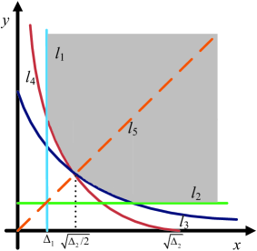
Figure 12: The integral region for $\mathbb{P}_{2}$, where ${\Delta_{\rm{1}}}<\sqrt{{\Delta_{\rm{2}}}{\rm{/2}}}$.

ii): When ${\Delta_{\rm{1}}}<\sqrt{{\Delta_{\rm{2}}}{\rm{/2}}}$ holds, the integral region for $\mathbb{P}_{2}$ can be shown as the shadow area in Fig. 12 at the top of the next page. Hence, $\mathbb{P}_{2}$ can be expressed as ${\mathbb{P}_{2}^{2}}$, given by

$$\mathbb{P}_{2}^{2}= \underbrace{\int_{\sqrt{{\Delta_{2}}/2}}^{\Phi}{\int_{Q\left(x\right)}^{x}{{f_{Y}}\left(y\right){f_{X}}\left(x\right)dydx}}}_{\mathbb{P}_{2,1}^{2}}$$

$$+\underbrace{\int_{\Phi}^{\infty}{\int_{{\Delta_{1}}}^{x}{{f_{Y}}\left(y\right){f_{X}}\left(x\right)dydx}}}_{\mathbb{P}_{2,2}^{2}}$$

$$+\underbrace{\int_{\sqrt{{\Delta_{2}}/2}}^{\Phi}{\int_{Q\left(y\right)}^{y}{{f_{X}}\left(x\right){f_{Y}}\left(y\right)dxdy}}}_{\mathbb{P}_{2,3}^{2}}$$

$$+\underbrace{\int_{\Phi}^{\infty}{\int_{{\Delta_{1}}}^{y}{{f_{X}}\left(x\right){f_{Y}}\left(y\right)dx}}dy}_{\mathbb{P}_{2,4}^{2}},$$ (B.6)

where $\Phi=-{\Delta_{1}}+{\Delta_{2}}/{\Delta_{1}}$, $Q\left(x\right)=\left({-x+\sqrt{{x^{2}}+4{\Delta_{2}}}}\right)/2$ and $Q\left(y\right)=\left({-y+\sqrt{{y^{2}}+4{\Delta_{2}}}}\right)/2$.

By means of variable substitution, $\mathbb{P}_{2,1}^{2}$ can be expressed as

$$\mathbb{P}_{2,1}^{2}=\int_{0}^{\Phi-\sqrt{{\Delta_{2}}/2}}{\frac{1}{{\Gamma\left({{m_{a}}}\right)\Gamma\left({{m_{b}}}\right)\theta_{a}^{{m_{a}}}}}}$$

$$\!\times\!{{\left(\!{x\!+\!\sqrt{{\Delta_{2}}/2}}\!\right)}^{{m_{a}}\!-\!1}}{e^{\!-\!\frac{{x\!+\!\sqrt{{\Delta_{2}}/2}}}{{{\theta_{a}}}}}}\Bigg{(}\gamma\left(\!{{m_{b}},\frac{{x\!+\!\sqrt{{\Delta_{2}}/2}}}{{{\theta_{b}}}}}\!\right)$$

$$-\gamma\left({{m_{b}},\frac{{Q\left({x+\sqrt{{\Delta_{2}}/2}}\right)}}{{{\theta_{b}}}}}\right)\Bigg{)}dx.$$ (B.7)

According to [29, 8.352.6], $\mathbb{P}_{2,1}^{2}$ can be rewritten as (B), as presented at the top of the next page. Due to the high complexity for the integral in ${\Xi_{3}}$, we adopt the Guassian-Chebyshev quadrature⁷ to approximate it. Thus, the first term of $\mathbb{P}_{2,1}^{2}$, ${\Xi_{3}}$, can be calculated as

$${\Xi_{3}}= \frac{{\pi\left({\Phi-\sqrt{{\Delta_{2}}/2}}\right)}}{{2N\Gamma\left({{m_{a}}}\right)\theta_{a}^{{m_{a}}}}}\sum\limits_{l=0}^{{m_{b}}-1}{\sum\limits_{n=1}^{N}{\sqrt{1-v_{n}^{2}}\frac{1}{{l!}}{{\left({\frac{1}{{{\theta_{b}}}}}\right)}^{l}}}}$$

$$\times{\left({k_{n}^{{}^{\prime}}+\sqrt{{\Delta_{2}}/2}}\right)^{{m_{a}}-1}}{Q^{l}}\left({k_{n}^{{}^{\prime}}+\sqrt{{\Delta_{2}}/2}}\right)$$

$$\times{e^{-\frac{{k_{n}^{{}^{\prime}}+\sqrt{{\Delta_{2}}/2}}}{{{\theta_{a}}}}-\frac{{Q\left({k_{n}^{{}^{\prime}}+\sqrt{{\Delta_{2}}/2}}\right)}}{{{\theta_{b}}}}}},$$ (B.9)

where ${v_{n}}=\cos\left({\frac{{\left({2n-1}\right)\pi}}{{2N}}}\right)$, $k_{n}^{{}^{\prime}}=\frac{{\Phi-\sqrt{{\Delta_{2}}/2}}}{2}\left({{v_{n}}+1}\right)$ and $N$ is the complexity and accuracy tradeoff parameter.

Adopting variable substitution, the second term of $\mathbb{P}_{2,1}^{2}$, ${\Xi_{4}}$, can be written as

$${\Xi_{4}}\!=\!\frac{1}{{\Gamma\left(\!{{m_{a}}}\!\right)\theta_{a}^{{m_{a}}}}}\sum\limits_{l\!=\!0}^{{m_{b}}\!-\!1}{\frac{1}{{l!}}}{\left(\!{\frac{1}{{{\theta_{b}}}}}\!\right)^{l}}{\left(\!{\frac{{{\theta_{a}}{\theta_{b}}}}{{{\theta_{a}}\!+\!{\theta_{b}}}}}\!\right)^{{m_{a}}\!+\!l}}\;\;\;\;\;\;\;\;\;\;\;\;$$

$$\times{e^{-\sqrt{{\Delta_{2}}/2}\left({\frac{1}{{{\theta_{a}}}}+\frac{1}{{{\theta_{b}}}}}\right)}}\int_{0}^{\left({\frac{1}{{{\theta_{a}}}}+\frac{1}{{{\theta_{b}}}}}\right)\left({\Phi-\sqrt{{\Delta_{2}}/2}}\right)}$$

$$\!\times\!{\left(\!{x\!+\!\sqrt{{\Delta_{2}}/2}\left(\!{\frac{1}{{{\theta_{a}}}}+\frac{1}{{{\theta_{b}}}}}\right)}\right)^{{m_{a}}+l-1}}{e^{-x}}dx.$$ (B.10)

Using [29, 3.382.5], ${\Xi_{4}}$ can be calculated as

$${\Xi_{4}}= \frac{1}{{\Gamma\left({{m_{a}}}\right)\theta_{a}^{{m_{a}}}}}\sum\limits_{l=0}^{{m_{b}}-1}{\frac{1}{{l!}}}{\left({\frac{1}{{{\theta_{b}}}}}\right)^{l}}{\left({\frac{{{\theta_{a}}{\theta_{b}}}}{{{\theta_{a}}+{\theta_{b}}}}}\right)^{{m_{a}}+l}}$$

$$\times\bigg{(}\gamma\left({{m_{a}}+l,\Phi\left({\frac{1}{{{\theta_{a}}}}+\frac{1}{{{\theta_{b}}}}}\right)}\right)$$

$$-\gamma\left({{m_{a}}+l,\sqrt{{\Delta_{2}}/2}\left({\frac{1}{{{\theta_{a}}}}+\frac{1}{{{\theta_{b}}}}}\right)}\right)\bigg{)}.$$ (B.11)

On the basis of the derivation of ${\mathbb{P}_{2}^{1}}$, $\mathbb{P}_{2,2}^{2}$ can be calculated as

$$\mathbb{P}_{2,2}^{2}=\frac{1}{{\Gamma\left({{m_{a}}}\right)}}\Gamma\left({{m_{a}},\Phi/{\theta_{a}}}\right)-\frac{1}{{\Gamma\left({{m_{a}}}\right)\theta_{a}^{{m_{a}}}}}\sum\limits_{l=0}^{{m_{b}}-1}{\frac{1}{{l!}}}$$

$$\!\times\!{\left(\!{\frac{1}{{{\theta_{b}}}}}\!\right)^{l}}{\left(\!{\frac{1}{{{\theta_{a}}}}\!+\!\frac{1}{{{\theta_{b}}}}}\!\right)^{\!-\!\left({l\!+\!{m_{a}}}\right)}}\Gamma\left({l\!+\!{m_{a}},\Phi\left({\frac{1}{{{\theta_{a}}}}\!+\!\frac{1}{{{\theta_{b}}}}}\right)}\right)$$

$$\!-\!\frac{1}{{\Gamma\left({{m_{b}}}\right)}}\gamma\left({{m_{b}},{\Delta_{1}}/{\theta_{b}}}\right)\left({1\!-\!\frac{1}{{\Gamma\left(\!{{m_{a}}}\right)}}\gamma\left(\!{{m_{a}},\Phi/{\theta_{a}}}\!\right)}\!\right).$$ (B.12)

In addition, referring to the analyses of ${\mathbb{P}_{2,1}^{2}}$ and ${\mathbb{P}_{2,2}^{2}}$, we can also derive ${\mathbb{P}_{2,3}^{2}}$ and ${\mathbb{P}_{2,4}^{2}}$ in closed-forms respectively. Based on the above derivation, the closed-form expression for ${\mathbb{P}_{2}^{2}}$ can be obtained as (III-A).

Appendix C

According to (22), the diversity gain can be calculated respectively in the two cases as follows.

i): When ${\gamma_{th}}\geq\frac{1}{{k_{1}^{2}+k_{2}^{2}}}$ is satisfied, $d=-\mathop{\lim}\limits_{\rho\to\infty}\frac{{\log\left({\rm{1}}\right)}}{{\log\left(\rho\right)}}{\rm{=0}}$;

ii): When ${\gamma_{th}}<\frac{1}{{k_{1}^{2}+k_{2}^{2}}}$ holds, the diversity gain can be expressed as

$$d=-\underbrace{\mathop{\lim}\limits_{\rho\to\infty}\frac{{\log\left({\mathbb{P}_{1}^{1}}\right)}}{{\log\left(\rho\right)}}}_{{\Xi_{5}}}-\underbrace{\mathop{\lim}\limits_{\rho\to\infty}\frac{{\log\left(1-{\mathbb{P}_{2}^{*}}\right)}}{{\log\left(\rho\right)}}}_{{\Xi_{6}}}.$$ (C.1)

Using [29, 8.352.6] and $\gamma\left({n,z}\right)\mathop{\simeq}\limits^{z\to 0}{z^{n}}/n$ [28], the first term of (C.1), ${\Xi_{5}}$, can be calculated as

$${\Xi_{5}} =\mathop{\lim}\limits_{\rho\to\infty}\frac{{\log\left({{{\left({\frac{{{\gamma_{th}}}}{{{\theta_{d}}\rho\left({1-{\gamma_{th}}\left({k_{1}^{2}+k_{2}^{2}}\right)}\right)}}}\right)}^{{m_{d}}}}/{m_{d}}!}\right)}}{{\log\left(\rho\right)}}$$

$$=-{m_{d}}.$$ (C.2)

According to the discussion in Appendix B, as the input SNR $\rho$ approaches infinity, $\mathbb{P}_{2}^{*}\approx\mathbb{P}_{2}^{1}$ holds. Moreover, a careful observation of (II-B) reveals that the probability $\mathbb{P}_{2}^{1}(\rho)$ increases with $\mathbb{P}_{2}^{1}(\rho)\propto\frac{1}{{\Gamma\left(\Lambda\right)}}\Gamma\left({\Lambda,{\Delta_{1}}/{\theta_{i}}}\right)$, where $\Lambda=\min\left({{m_{a}},{m_{b}}}\right)$, ${\Delta_{1}}=\frac{{{\gamma_{th}}}}{{\left({1-\beta}\right)\left({1-\left({k_{1}^{2}+k_{2}^{2}}\right){\gamma_{th}}}\right)\rho}}$ and when $\Lambda={m_{a}}\left({{m_{b}}}\right)$, $i=a(b)$. Hence, the second term of (C.1), ${\Xi_{6}}$, can be approximated as

$${\Xi_{6}}\approx\mathop{\lim}\limits_{\rho\to\infty}\frac{{\log\left({1-\frac{1}{{\Gamma\left(\Lambda\right)}}\Gamma\left({\Lambda,{\Delta_{1}}/{\theta_{i}}}\right)}\right)}}{{\log\left(\rho\right)}}.$$ (C.3)

Similar to the derivation of ${\Xi_{5}}$, we can obtain ${\Xi_{6}}=-\min\left({{m_{a}},{m_{b}}}\right)$.

Based on the above discussions, the diversity gain can be obtained as (24).

References

- [1] Y. Yang, H. Hu, J. Xu, and G. Mao, “Relay technologies for WiMAX and LTE-advanced mobile systems,” IEEE Commun. Mag., vol. 47, no. 10, pp. 100–105, Oct. 2009.
- [2] A. A. Nasir, X. Zhou, S. Durrani, and R. A. Kennedy, “Relaying protocols for wireless energy harvesting and information processing,” IEEE Trans. Wireless Commun., vol. 12, no. 7, pp. 3622–3636, Jul. 2013.
- [3] I. Krikidis, S. Timotheou, S. Nikolaou, G. Zheng, D. W. K. Ng, and R. Schober, “Simultaneous wireless information and power transfer in modern communication systems,” IEEE Commun. Mag., vol. 52, no. 11, pp. 104–110, Nov. 2014.
- [4] N. T. P. Van, S. F. Hasan, X. Gui, S. Mukhopadhyay, and H. Tran, “Three-step two-way decode and forward relay with energy harvesting,” IEEE Commun. Lett., vol. 21, no. 4, pp. 857–860, Apr. 2017.
- [5] T. P. Do, I. Song, and Y. H. Kim, “Simultaneous wireless transfer of power and information in a decode-and-forward two-way relaying network,” IEEE Trans. Wireless Commun., vol. 16, no. 3, pp. 1579–1592, Mar. 2017.
- [6] L. Shi, Y. Ye, R. Q. Hu, and H. Zhang, “System outage performance for three-step two-way energy harvesting DF relaying,” IEEE Trans. Veh. Technol., vol. 68, no. 4, pp. 3600–3612, Apr. 2019.
- [7] S. Modem and S. Prakriya, “Performance of analog network coding based two-way EH relay with beamforming,” IEEE Trans. Wireless Commun., vol. 65, no. 4, pp. 1518–1535, Apr. 2017.
- [8] C. In, H. Kim, and W. Choi, “Achievable rate-energy region in two-way decode-and-forward energy harvesting relay systems,” IEEE Trans. Commun., vol. 67, no. 6, pp. 3923–3935, Jun. 2019.
- [9] A. Mukherjee, T. Acharya, and M. R. A. Khandaker, “Outage analysis for SWIPT-enabled two-way cognitive cooperative communications,” IEEE Trans. Veh. Technol., vol. 67, no. 9, pp. 9032–9036, Sep. 2018.
- [10] S. Singh, S. Modem, and S. Prakriya, “Optimization of cognitive two-way networks with energy harvesting relays,” IEEE Commun. Lett., vol. 21, no. 6, pp. 1381–1384, 2017.
- [11] V. N. Quoc Bao, H. Van Toan, and K. N. Le, “Performance of two-way AF relaying with energy harvesting over Nakagami-m fading channels,” IET Commun., vol. 12, no. 20, pp. 2592–2599, 2018.
- [12] Y. Ye, L. Shi, X. Chu, H. Zhang, and G. Lu, “On the outage performance of SWIPT-based three-step two-way DF relay networks,” IEEE Trans. Veh. Technol., vol. 68, no. 3, pp. 3016–3021, Mar. 2019.
- [13] L. Shi, Y. Ye, X. Chu, Y. Zhang, and H. Zhang, “Optimal combining and performance analysis for two-way EH relay systems with TDBC protocol,” IEEE Wireless Commun. Lett., vol. 8, no. 3, pp. 713–716, Jun. 2019.
- [14] Y. Ye, Y. Li, Z. Wang, X. Chu, and H. Zhang, “Dynamic asymmetric power splitting scheme for SWIPT-based two-way multiplicative AF relaying,” IEEE Signal Process. Lett., vol. 25, no. 7, pp. 1014–1018, Jul. 2018.
- [15] J. Qi, S. Aissa, and M. Alouini, “Analysis and compensation of I/Q imbalance in amplify-and-forward cooperative systems,” in Proc. IEEE WCNC, pp. 215–220, Apr. 2012.
- [16] E. Björnson, M. Matthaiou, and M. Debbah, “A new look at dual-hop relaying: Performance limits with hardware impairments,” IEEE Trans. Commun., vol. 61, no. 11, pp. 4512–4525, Nov. 2013.
- [17] B. Li, Y. Zou, J. Zhu, and W. Cao, “Impact of hardware impairment and co-channel interference on security-reliability trade-off for wireless sensor networks,” IEEE Trans. Wireless Commun., 2021.
- [18] H. Shen, W. Xu, S. Gong, C. Zhao, and D. W. K. Ng, “Beamforming optimization for irs-aided communications with transceiver hardware impairments,” IEEE Trans. Commun., vol. 69, no. 2, pp. 1214–1227, Feb. 2021.
- [19] D. K. Nguyen, M. Matthaiou, T. Q. Duong, and H. Ochi, “RF energy harvesting two-way cognitive DF relaying with transceiver impairments,” in Proc. IEEE ICC Workshop, pp. 1970–1975, Jun. 2015.
- [20] D. K. Nguyen, D. N. K. Jayakody, S. Chatzinotas, J. S. Thompson, and J. Li, “Wireless energy harvesting assisted two-way cognitive relay networks: Protocol design and performance analysis,” IEEE Access, vol. 5, pp. 21 447–21 460, 2017.
- [21] S. Solanki, V. Singh, and P. K. Upadhyay, “RF energy harvesting in hybrid two-way relaying systems with hardware impairments,” IEEE Trans. Veh. Technol., vol. 68, no. 12, pp. 11 792–11 805, Dec. 2019.
- [22] Z. Liu, G. Lu, Y. Ye, and X. Chu, “System outage probability of PS-SWIPT enabled two-way AF relaying with hardware impairments,” IEEE Trans. Veh. Technol., vol. 69, no. 11, pp. 13 532–13 545, 2020.
- [23] X. Li, J. Li, Y. Liu, Z. Ding, and A. Nallanathan, “Residual transceiver hardware impairments on cooperative NOMA networks,” IEEE Trans. Wireless Commun., vol. 19, no. 1, pp. 680–695, Jan. 2020.
- [24] Z. Zhou, M. Peng, Z. Zhao, and Y. Li, “Joint power splitting and antenna selection in energy harvesting relay channels,” IEEE Signal Process. Lett., vol. 22, no. 7, pp. 823–827, Jul. 2015.
- [25] Q. Liu, T. Lv, and Z. Lin, “Energy-efficient transmission design in cooperative relaying systems using noma,” IEEE Commun. Lett., vol. 22, no. 3, pp. 594–597, Mar. 2018.
- [26] X. Yue, Y. Liu, S. Kang, A. Nallanathan, and Z. Ding, “Exploiting full/half-duplex user relaying in NOMA systems,” IEEE Trans. Commun., vol. 66, no. 2, pp. 560–575, Feb. 2018.
- [27] L. Shi, R. Q. Hu, Y. Ye, and H. Zhang, “Modeling and performance analysis for ambient backscattering underlaying cellular networks,” IEEE Trans. Veh. Technol., vol. 69, no. 6, pp. 6563–6577, Jun. 2020.
- [28] S. Modem and S. Prakriya, “Performance of EH protocols in two-hop networks with a battery-assisted EH relay,” IEEE Trans. Veh. Technol., vol. 67, no. 10, pp. 10 022–10 026, Oct. 2018.
- [29] I. S. Gradshteyn and I. M. Ryzhik, Table of Integrals, Series, and Products, 7th ed. New York, NY, USA: Academic, 2007.