Zai Shi*zaishi@ethz.ch1 Zhao Meng*zhmeng@ethz .ch1 Yiran Xingyiran.xing@rwth-aachen.de2 Yunpu Macognitive.yunpu@gmail.com3 Roger Wattenhoferwattenhofer@ethz.ch1 ETH Zurich RWTH Aachen LMU Munich 3D-RETR

3D-RETR: End-to-End Single and Multi-View 3D Reconstruction with Transformers

3D reconstruction aims to reconstruct 3D objects from 2D views. Previous works for 3D reconstruction mainly focus on feature matching between views or using CNNs as backbones. Recently, Transformers have been shown effective in multiple applications of computer vision. However, whether or not Transformers can be used for 3D reconstruction is still unclear. In this paper, we fill this gap by proposing 3D-RETR, which is able to perform end-to-end 3D REconstruction with TRansformers. 3D-RETR first uses a pretrained Transformer to extract visual features from 2D input images. 3D-RETR then uses another Transformer Decoder to obtain the voxel features. A CNN Decoder then takes as input the voxel features to obtain the reconstructed objects. 3D-RETR is capable of 3D reconstruction from a single view or multiple views. Experimental results on two datasets show that 3D-RETR reaches state-of-the-art performance on 3D reconstruction. Additional ablation study also demonstrates that 3D-DETR benefits from using Transformers.

1 Introduction

3D reconstruction focuses on using a single or multiple 2D images of an object to rebuild its 3D representations. 3D reconstruction has played an important role in various downstream applications, including CAD [Avetisyan et al.(2019)Avetisyan, Dahnert, Dai, Savva, Chang, and Nießner], human detection [Popa et al.(2017)Popa, Zanfir, and Sminchisescu], architecture [Hermoza and Sipiran(2018)], etc. The wide applications of 3D reconstruction have motivated researchers to develop numerous methods for 3D reconstruction. Early works for 3D reconstruction mostly use feature matching between different views of an object [Dissanayake et al.(2001)Dissanayake, Newman, Clark, Durrant-Whyte, and Csorba, Geiger et al.(2011)Geiger, Ziegler, and Stiller, Cheng et al.(2014)Cheng, Leng, Wu, Cui, and Lu]. However, the performance of such methods largely depends on accurate and consistent margins between different views of objects and are thus vulnerable to rapid changes between views [Lowe(2004), Bhat and Nayar(1998), Saponaro et al.(2014)Saponaro, Sorensen, Rhein, Mahoney, and Kambhamettu]. Additionally, these methods are not suitable for single-view 3D reconstruction, where only one view of an object is available.

The advances of deep learning have shed some light on neural network-based approaches for 3D reconstruction [Han et al.(2019)Han, Laga, and Bennamoun]. On the one hand, some researchers formulate 3D reconstruction as a sequence learning problem and use recurrent neural networks to solve the problem [Choy et al.(2016)Choy, Xu, Gwak, Chen, and Savarese, Kar et al.(2017)Kar, Häne, and Malik]. On the other hand, other researchers employ the encoder-decoder architecture for 3D reconstruction [Tulsiani et al.(2018)Tulsiani, Efros, and Malik, Xie et al.(2019)Xie, Yao, Sun, Zhou, and Zhang]. Furthermore, researchers have also used Generative Adversarial Networks (GANs) for 3D reconstruction [Jiang et al.(2018)Jiang, Shi, Qi, and Jia]. However, these approaches often rely on sophisticated pipelines of convolutional neural networks (CNNs), and build models with large amounts of parameters, which are computationally expensive.

Recently, Transformers [Vaswani et al.(2017)Vaswani, Shazeer, Parmar, Uszkoreit, Jones, Gomez, Kaiser, and Polosukhin] have gained attention from the computer vision community. Transformer-based models have achieved state-of-the-art performance in many downstream applications of computer vision, including image classification [Dosovitskiy et al.(2021)Dosovitskiy, Beyer, Kolesnikov, Weissenborn, Zhai, Unterthiner, Dehghani, Minderer, Heigold, Gelly, Uszkoreit, and Houlsby], semantic segmentation [Liu et al.(2021)Liu, Lin, Cao, Hu, Wei, Zhang, Lin, and Guo], image super-resolution [Yang et al.(2020)Yang, Yang, Fu, Lu, and Guo], etc. Despite these achievements, whether or not Transformers can be used in 3D reconstruction is still unclear.

In this paper, we propose 3D-RETR, which is capable of performing end-to-end single and multi-view 3D REconstruction with TRansformers. 3D-RETR uses a pretrained Transformer to extract visual features from 2D images. 3D-RETR then obtains the 3D voxel features by using another Transformer Decoder. Finally, a CNN Decoder outputs the 3D representation from the voxel features. Our contributions in this paper are three-folded:

• We propose 3D-RETR for end-to-end single and multi-view 3D reconstruction with Transformers. To the best of our knowledge, we are the first to use Transformers for end-to-end 3D reconstruction. Experimental results show that 3D-RETR reaches state-of-the-art performance under both synthetic and real-world settings.

• We conduct additional ablation studies to understand how each part of 3D-RETR contributes to the final performance. The experimental results show that our choices of the encoder, decoder, and loss are beneficial.

• 3D-RETR is efficient compared to previous models. 3D-RETR reaches higher performance than previous models, despite that it uses far fewer parameters.

2 Related Work

In this Section, we briefly review previous works. Section 2.1 gives an overview of previous works on 3D reconstruction. Section 2.2 introduces Transformers.

2.1 3D reconstruction

3D reconstruction has been widely used in various downstream applications, including architecture [Hermoza and Sipiran(2018)], CAD [Avetisyan et al.(2019)Avetisyan, Dahnert, Dai, Savva, Chang, and Nießner], human detection [Popa et al.(2017)Popa, Zanfir, and Sminchisescu], etc. Researchers have mainly focused on two types of methods for 3D reconstruction. Some researchers use depth cameras such as Kinect to collect images with depth information [Izadi et al.(2011)Izadi, Kim, Hilliges, Molyneaux, Newcombe, Kohli, Shotton, Hodges, Freeman, Davison, et al.], which is subsequently processed for 3D reconstruction. However, such methods require sophisticated hardware and data collection procedures and are thus not practical in many scenarios.

To mitigate this problem, other researchers have resorted to 3D reconstruction from single or multiple views, where only 2D images are available. Early researchers leverage feature matching between different views for 3D reconstruction with 2D images. For example, [Agarwal et al.(2009)Agarwal, Snavely, Simon, Seitz, and Szeliski] uses a multi-stage parallel matching algorithm for feature matching, and [Cheng et al.(2014)Cheng, Leng, Wu, Cui, and Lu] proposes a cascade hashing strategy for efficient image matching and 3D reconstruction. Although these methods are useful, their performance degrades when margins between different views are large, making these methods hard to generalize.

Recent works mainly focus on neural network-based approaches. Some researchers have formulated multi-view 3D construction as a sequence learning problem. For example, [Choy et al.(2016)Choy, Xu, Gwak, Chen, and Savarese] proposes a 3D recurrent neural network, which takes as input one view at each timestep and outputs the reconstructed object representation. Others employ an encoder-decoder architecture by first encoding the 2D images into fixed-size vectors, from which a decoder decodes the 3D representations [Tulsiani et al.(2018)Tulsiani, Efros, and Malik, Xie et al.(2019)Xie, Yao, Sun, Zhou, and Zhang, Tulsiani et al.(2017b)Tulsiani, Zhou, Efros, and Malik]. Furthermore, researchers have also used Generative Adversarial Networks (GANs) [Jiang et al.(2018)Jiang, Shi, Qi, and Jia] and 3D-VAEs [Soltani et al.(2017)Soltani, Huang, Wu, Kulkarni, and Tenenbaum, Mandikal et al.(2018)Mandikal, L., Agarwal, and Radhakrishnan] for 3D reconstruction. However, these neural network-based methods often rely on sophisticated pipelines of different convolutional neural networks, and are often with models of large amounts of parameters, which are computationally expensive.

2.2 Transformers

Researchers first propose Transformers for applications in natural language processing [Vaswani et al.(2017)Vaswani, Shazeer, Parmar, Uszkoreit, Jones, Gomez, Kaiser, and Polosukhin], including machine translation, language modeling, etc. Transformers use a multi-head self-attention mechanism, in which inputs from a specific time step would attend to the entire input sequence.

Recently, Transformers have also gained attention from the computer vision community. In image classification, Vision Transformer (ViT) [Dosovitskiy et al.(2021)Dosovitskiy, Beyer, Kolesnikov, Weissenborn, Zhai, Unterthiner, Dehghani, Minderer, Heigold, Gelly, Uszkoreit, and Houlsby] reach state-of-the-art performance on image classification by feeding images as patches into a Transformer. DeiT [Touvron et al.(2021)Touvron, Cord, Douze, Massa, Sablayrolles, and Jégou] achieves better performance than ViT [Dosovitskiy et al.(2021)Dosovitskiy, Beyer, Kolesnikov, Weissenborn, Zhai, Unterthiner, Dehghani, Minderer, Heigold, Gelly, Uszkoreit, and Houlsby] with much less pretraining data and a smaller parameter size. Transformers are also useful in other computer vision applications. For example, DETR [Carion et al.(2020)Carion, Massa, Synnaeve, Usunier, Kirillov, and Zagoruyko], consisting of a Transformer Encoder and a Transformer Decoder, has reached state-of-the-art performance on object detection. Other applications of Transformers also include super-resolution [Yang et al.(2020)Yang, Yang, Fu, Lu, and Guo], semantic segmentation [Liu et al.(2021)Liu, Lin, Cao, Hu, Wei, Zhang, Lin, and Guo], video understanding [Wang et al.(2021)Wang, Xu, Wang, Shen, Cheng, Shen, and Xia], etc.

In this paper, we propose 3D-RETR for end-to-end single and multi-view 3D reconstruction. 3D-RETR consists of a Transformer Encoder, a Transformer Decoder, and another CNN Decoder. We show in our experiments (see Section 4) that 3D-RETR reaches state-of-the-art performance, while using much fewer parameters than previous models, including pix2vox++ [Xie et al.(2020)Xie, Yao, Zhang, Zhou, and Sun], 3D-R2N2 [Choy et al.(2016)Choy, Xu, Gwak, Chen, and Savarese], etc.

2.3 Differentiable Rendering

Recently, differentiable rendering methods like SRN [Sitzmann et al.(2019)Sitzmann, Zollhöfer, and Wetzstein], DVR [Niemeyer et al.(2020)Niemeyer, Mescheder, Oechsle, and Geiger], NeRF [Mildenhall et al.(2020)Mildenhall, Srinivasan, Tancik, Barron, Ramamoorthi, and Ng], and IDR [Yariv et al.(2020)Yariv, Kasten, Moran, Galun, Atzmon, Ronen, and Lipman] have become popular. These methods implicitly represent the scene using deep neural networks and have achieved impressive results. However, these methods need to evaluate their neural network thousands of times to extract geometry, which results in a long inference time.

In contrast, our method, along with other previous 3D reconstruction methods including 3D-R2N2 [Choy et al.(2016)Choy, Xu, Gwak, Chen, and Savarese], OGN [Tatarchenko et al.(2017)Tatarchenko, Dosovitskiy, and Brox] and pix2vox [Xie et al.(2019)Xie, Yao, Sun, Zhou, and Zhang], aims to reconstruct the volume without rendering the 2D images. 3D-RETR learns the 3D shape prior out of input 2D images and generates 3D-voxels during the inference time.

3 Methodology

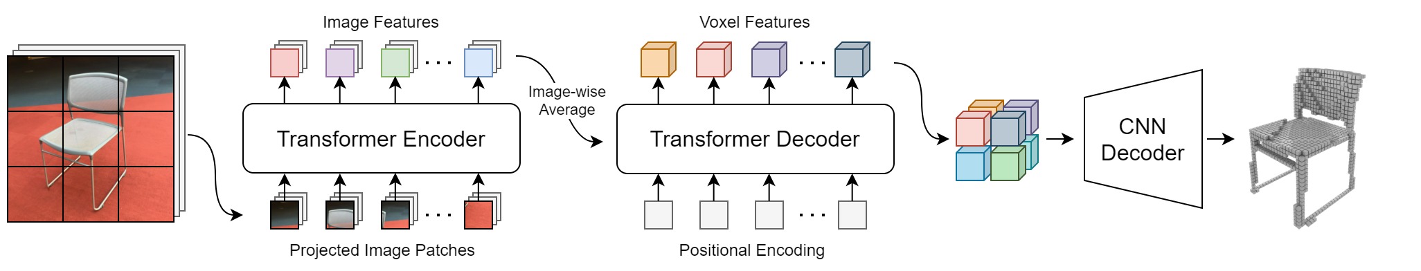
Figure 1: An illustration of our 3D-RETR. A Transformer Encoder firsts extract image features from 2D images. 3D-RETR then obtain the voxel features by using another Transformer Decoder. A CNN Decoder finally outputs the 3D object representation.

From a high level, 3D-RETR consists of three main components (see Figure 1): a Transformer Encoder, a Transformer Decoder, and a CNN Decoder. The Transformer Encoder takes as input the images, which are subsequently encoded into fixed-size image feature vectors. Then, the Transformer Decoder obtains voxel features by cross-attending to the image features. Finally, the CNN Decoder decodes 3D object representations from the voxel features. Figure 1 illustrates the architecture of 3D-RETR.

In this paper, we have two variants of 3D-RETR: (1) The base model, 3D-RETR-B, has 163M parameters; (2) The smaller model, 3D-RETR-S, has 11M parameters. We describe the details of these two models in Section 4.

We denote the input images of an object from $V$ different views as $x_{1},\ldots,x_{V}\in\mathbb{R}^{C\times H\times W}$, where $C=3$ is the RGB channel, and $H$ and $W$ are the height and width of the images, respectively. We denote the reconstructed voxel by $Y=\{y_{1},y_{2},\cdots,y_{N^{3}}|y_{i}\in\{0,1\},1\leq i\leq N^{3}\}$, where $i$ is the index to the voxel grids, $0$ indicates an empty voxel grid, $1$ indicates an occupied grid, and $N$ is the resolution of the voxel representation.

3.1 Transformer Encoder

A Vision Transformer takes as input image $x_{i}$ by splitting the image into $B^{2}$ patches. At each time step, the corresponding patch is embedded by first linearly transformed into a fixed-size vector, which is then added with positional embeddings. The Transformer takes the embedded patch feature as input and outputs $B^{2}$ encoded dense image feature vectors. For single-view reconstruction, we keep all the $B^{2}$ dense image vectors. For multi-view reconstruction, at each time step, we take the average across different views, and keep the averaged $B^{2}$ dense vectors.

In our implementation, we use the Data-efficient image Transformer (DeiT) [Touvron et al.(2021)Touvron, Cord, Douze, Massa, Sablayrolles, and Jégou]. Our base model, 3D-RETR-B, uses the DeiT Base (DeiT-B) as the Transformer Encoder. DeiT-B consists of 12 layers, each of which has 12 heads and 768-dimensional hidden embeddings. The smaller model, 3D-RETR-S, uses the DeiT Tiny (DeiT-Ti) as the Transformer Encoder. DeiT-Ti has 12 layers, each of which has 3 heads and 192-dimensional hidden embeddings. Both 3D-RETR-B and 3D-RETR-S have $B=16$. We feed all $B^{2}$ dense image vectors in the next stage into the Transformer Decoder, which we introduce in Section 3.2.

3.2 Transformer Decoder

The Transformer Decoder takes $M^{3}$ learned positional embeddings as its input and cross-attends to the output of the Transformer Encoder. Our Transformer Decoder is similar to that of DETR [Carion et al.(2020)Carion, Massa, Synnaeve, Usunier, Kirillov, and Zagoruyko], where the Transformer decodes all input vectors in parallel, instead of autoregressively as in the original Transformer [Vaswani et al.(2017)Vaswani, Shazeer, Parmar, Uszkoreit, Jones, Gomez, Kaiser, and Polosukhin].

The 3D-RETR-B model has a Transformer Decoder of 8 layers, each of which has 12 heads and 768-dimensional hidden embeddings. For the 3D-RETR-S, we use a Transformer Decoder of $6$ layers, each of which 3 heads and 192-dimensional hidden embeddings. To enable the Transformer Decoder to understand the spatial relations between voxel features, we create $M^{3}$ positional embeddings for the Transformer Decoder. The positional embeddings are learnable and are updated during training. We use $M=4$ for both 3D-RETR-B and 3D-RETR-S.

3.3 CNN Decoder

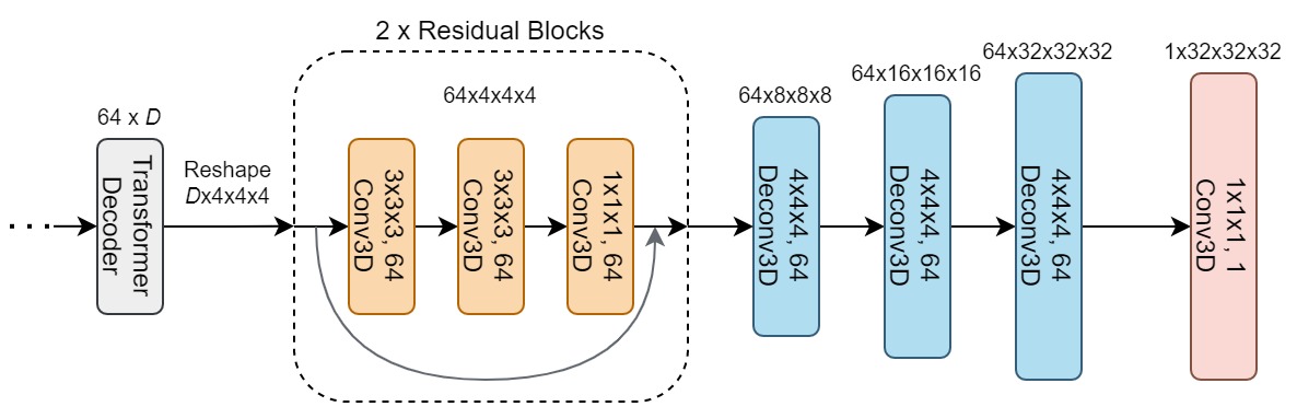
Figure 2: Details of the CNN Decoder in 3D-RETR. The CNN Decoder consists of two residual blocks and three transposed 3D convolutional layers. $D$ is the hidden size of the Transformer.

The CNN Decoder takes as input the voxel features from the Transformer Decoder and outputs the voxel representation. As the Transformer Encoder and Transformer Decoder already give rich information, we use a relatively simple architecture for the CNN Decoder. The CNN Decoder first stacks the voxel feature vectors into a cube of size $M^{3}$, and then upsample the cube iteratively until the desired resolution is obtained.

Figure 2 illustrates the architecture of our CNN Decoder. Specifically, the CNN Decoder has two residual blocks [He et al.(2016)He, Zhang, Ren, and Sun], each consisting of four transposed 3D convolutional layers. For the residual blocks, the first two convolutional layers have a kernel size of 3, and the last one uses a kernel size of 1. In addition, all three layers have 64 channels. For the transposed 3D convolutional layers, all three layers have a kernel size of 4, a stride of 2, a channel size of 64, and a padding size of 1. We add an additional $1\times 1$ convolutional layer at the end of the CNN Decoder to compress the 64 channels into one channel. The model finally outputs cubes of size $32^{3}$.

3.4 Loss Function

While previous works on 3D reconstruction mainly use the cross-entropy loss, researchers have also shown that other losses such as Dice and Focal loss are better for optimizing IoUs [Sudre et al.(2017)Sudre, Li, Vercauteren, Ourselin, and Cardoso, Lin et al.(2020)Lin, Goyal, Girshick, He, and Dollár, Berman et al.(2018)Berman, Triki, and Blaschko]. Although these losses are originally proposed for 2D image tasks, they can be easily adapted to 3D tasks.

This paper uses Dice loss as the loss function, which is suitable for 3D reconstruction as the voxel occupancy is highly unbalanced. Formally, we have the Dice loss for the 3D voxels as follows:

$$\mathcal{L}_{Dice}=1-\frac{\sum_{n=1}^{N^{3}}p_{n}y_{n}}{\sum_{n=1}^{N^{3}}p_{n}+y_{n}}-\frac{\sum_{n=1}^{N^{3}}(1-p_{n})(1-y_{n})}{\sum_{n=1}^{N^{3}}2-p_{n}-y_{n}}$$

where $p_{n}$ is the $n$-th predicted probability of the voxel occupation and $y_{n}$ is the $n$-th ground-truth voxel.

3.5 Optimization

To train the 3D-RETR. We use the AdamW [Loshchilov and Hutter(2019)] optimizer with a learning rate of $1e-4$, $\beta_{1}=0.9$, $\beta_{2}=0.999$, and a weight decay of $1e-2$. The batch size is set to 16 for all the experiments. We use two RTX Titan GPUs in our experiments. Training takes 1 to 3 days, depending on the exact setting. We use mixed-precision to speed up training.

4 Experiments

We show in this Section our experimental results. We evaluate 3D-RETR on ShapeNet [Chang et al.(2015)Chang, Funkhouser, Guibas, Hanrahan, Huang, Li, Savarese, Savva, Song, Su, Xiao, Yi, and Yu] and Pix3d [Sun et al.(2018)Sun, Wu, Zhang, Zhang, Zhang, Xue, Tenenbaum, and Freeman]. Following previous works [Choy et al.(2016)Choy, Xu, Gwak, Chen, and Savarese, Xie et al.(2019)Xie, Yao, Sun, Zhou, and Zhang], we use Intersection of Union (IoU) as our evaluation metric.

4.1 ShapeNet

ShapeNet is a large-scale 3D object dataset consisting of $55$ object categories with $51,300$ 3D models. Following the setting in Pix2Vox [Xie et al.(2019)Xie, Yao, Sun, Zhou, and Zhang], we use the same subset of $13$ categories and about $44,000$ models. The 3D models are pre-processed using Binvox with a resolution of $32^{3}$. The images are then rendered in the resolution of $137\times 137$ from $24$ random views.

For single-view 3D reconstruction on ShapeNet, we compare our results with previous state-of-the-art models, including 3D-R2N2 [Choy et al.(2016)Choy, Xu, Gwak, Chen, and Savarese], OGN [Tatarchenko et al.(2017)Tatarchenko, Dosovitskiy, and Brox], Matryoshka Networks [Richter and Roth(2018)], AtlasNet [Groueix et al.(2018)Groueix, Fisher, Kim, Russell, and Aubry], Pixel2Mesh [Wang et al.(2018)Wang, Zhang, Li, Fu, Liu, and Jiang], OccNet [Mescheder et al.(2019)Mescheder, Oechsle, Niemeyer, Nowozin, and Geiger], IM-Net [Chen and Zhang(2019)], AttSets [Yang et al.(2019)Yang, Wang, Markham, and Trigoni], and Pix2Vox++ [Xie et al.(2020)Xie, Yao, Zhang, Zhou, and Sun]. Table 1 shows the results. We can observe that both 3D-RETR-S and 3D-RETR-B outperform all previous models in terms of overall IoU. Additionally, 3D-RETR-S outperforms all other baselines in 6 of the 13 categories, while 3D-RETR-B is the best among other baselines in 9 of the 13 categories.

Category	3D-R2N2	OGN	Matroyoshka	AtlasNet	Pixel2Mesh	OccNet	IM-Net	AttSets	Pix2Vox++	3D-RETR-S	3D-RETR-B
aeroplane	0.513	0.587	0.647	0.493	0.508	0.532	0.702	0.594	0.674	0.696	0.704
bench	0.421	0.481	0.577	0.431	0.379	0.597	0.564	0.552	0.608	0.643	0.650
cabinet	0.716	0.729	0.776	0.257	0.732	0.674	0.680	0.783	0.799	0.804	0.802
car	0.798	0.816	0.850	0.282	0.670	0.671	0.756	0.844	0.858	0.858	0.861
chair	0.466	0.483	0.547	0.328	0.484	0.583	0.644	0.559	0.581	0.579	0.592
display	0.468	0.502	0.532	0.457	0.582	0.651	0.585	0.565	0.548	0.576	0.574
lamp	0.381	0.398	0.408	0.261	0.399	0.474	0.433	0.445	0.457	0.463	0.483
rifle	0.544	0.593	0.616	0.573	0.468	0.656	0.723	0.601	0.721	0.665	0.668
sofa	0.628	0.646	0.681	0.354	0.622	0.669	0.694	0.703	0.725	0.729	0.735
speaker	0.662	0.637	0.701	0.296	0.672	0.655	0.683	0.721	0.617	0.719	0.724
table	0.513	0.536	0.573	0.301	0.536	0.659	0.621	0.590	0.620	0.615	0.633
telephone	0.661	0.702	0.756	0.543	0.762	0.794	0.762	0.743	0.809	0.796	0.781
watercraft	0.513	0.632	0.591	0.355	0.471	0.579	0.607	0.601	0.603	0.621	0.636
overall	0.560	0.596	0.635	0.352	0.552	0.626	0.659	0.642*	0.670*	0.674	0.680

Table 1: Results of single-view 3D reconstruction on the ShapeNet dataset. Bold is the best performance, while Italic is the second best. For overall IoU, we report the mean IoU across all 13 categories. However, for entries with $*$, the overall IoU is NOT the averaged IoU across categories. We nevertheless use the original number from Pix2Vox++ [Xie et al.(2020)Xie, Yao, Zhang, Zhou, and Sun] and AttSets [Yang et al.(2019)Yang, Wang, Markham, and Trigoni]. As a reference, the average IoU across categories for AttSets and Pix2Vox++ are $0.638$ and $0.663$, respectively.

For the multi-view setting, we take the number of input 2D images $V\in\{1,2,3,4,5,8,12,\\ 16,20\}$ and compare the performance of 3D-RETR with previous state-of-the-art models, including 3D-R2N2 [Choy et al.(2016)Choy, Xu, Gwak, Chen, and Savarese], AttSets [Yang et al.(2019)Yang, Wang, Markham, and Trigoni], and Pix2Vox++ [Xie et al.(2020)Xie, Yao, Zhang, Zhou, and Sun]. As we can see in Table 2, 3D-RETR outperforms all previous works on all different views. Furthermore, Figure 3 illustrates the relation between the number of views and model performance. One can observe that the performance of 3D-RETR increases rapidly compared to other methods as more views become available. Additionally, while models like 3D-R2N2 and AttSets gradually become saturated, our best model, 3D-RETR-B, continues to benefit from more views, indicating that 3D-RETR has a higher capacity.

As 3D-RETR simply takes the average over different views in the Transformer Encoder, we can train and evaluate 3D-RETR with different numbers of views. To understand how 3D-RETR performs when the number of views is different during training and evaluation, we conduct additional experiments to train 3D-RETR-B with 3 views and evaluate its performance under different numbers of views. We show the results in Table 2 (See the row of 3D-RETR-B (3 views)). Surprisingly, 3D-RETR-B still outperforms previous state-of-the-art models, even if the number of views during training and evaluation is different. In particular, the model seeing different numbers of views during training and evaluation demonstrates that 3D-RETR is flexible.

Model	1 view	2 views	3 views	4 views	5 views	8 views	12 views	16 views	20 views
3D-R2N2	0.560	0.603	0.617	0.625	0.634	0.635	0.636	0.636	0.636
AttSets	0.642	0.662	0.670	0.675	0.677	0.685	0.688	0.692	0.693
Pix2Vox++*	0.670	0.695	0.704	0.708	0.711	0.715	0.717	0.718	0.719
3D-RETR-S	0.674	0.695	0.707	0.715	0.719	0.728	0.734	0.737	0.738
3D-RETR-B (3 views)	0.674	0.707	0.716	0.720	0.723	0.727	0.729	0.730	0.731
3D-RETR-B	0.680	0.701	0.716	0.725	0.736	0.739	0.747	0.755	0.757

Table 2: Results of multi-view 3D reconstruction on the ShapeNet dataset. Our smallest model (3D-RETR-S) already reaches state-of-the-art performance. *: As mentioned in Table 1, while all other models report mean IoU across categories, Pix2Vox++ [Xie et al.(2020)Xie, Yao, Zhang, Zhou, and Sun] reports their overall IoU by taking the average across all the examples. For Pix2Vox++, we cannot compute mean IoU across different categories as Pix2Vox++ does not report per-category IoU for multi-view reconstruction.

Input	3D-R2N2	AtlasNet	OccNet	IM-NET	AttSets	Pix2Vox++	3D-RETR-S	3D-RETR-B	GT

Table 3: Examples of single-view 3D reconstruction from the ShapeNet dataset.

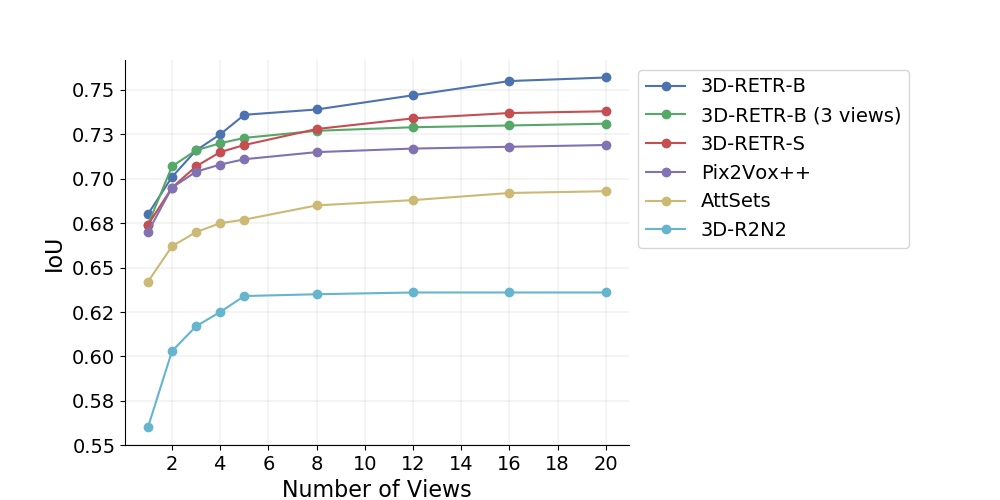
Figure 3: Model performance with different views. 3D-RETR-B continues to benefit from more views, while baselines including AttSets and Pix2Vox++ become saturated.

4.2 Pix3D

Different from ShapeNet, in which all examples are synthetic, Pix3D [Sun et al.(2018)Sun, Wu, Zhang, Zhang, Zhang, Xue, Tenenbaum, and Freeman] is a dataset of aligned 3D models and real-world 2D images. Evaluating models on Pix3D gives a better understanding of the model performance under practical settings. Following the same setting in Pix3D [Sun et al.(2018)Sun, Wu, Zhang, Zhang, Zhang, Xue, Tenenbaum, and Freeman], we use the subset consisting of 2,894 untruncated and unoccluded chair images as the test set. Moreover, we follow [Su et al.(2015)Su, Qi, Li, and Guibas] to synthesize 60 random images for each image in the ShapeNet-Chair category and use these synthesized images as our training set.

We compare 3D-RETR with previous state-of-art models, including DRC [Tulsiani et al.(2017a)Tulsiani, Zhou, Efros, and Malik], 3D-R2N2 [Choy et al.(2016)Choy, Xu, Gwak, Chen, and Savarese], Pix3D [Sun et al.(2018)Sun, Wu, Zhang, Zhang, Zhang, Xue, Tenenbaum, and Freeman], and Pix2Vox++ [Xie et al.(2020)Xie, Yao, Zhang, Zhou, and Sun]. Table 4 shows the results. 3D-RETR-B outperforms all previous models, and 3D-RETR-S reaches comparable performance despite that 3D-RETR-S is much smaller than 3D-RETR-B in terms of parameter size.

3D-R2N2	DRC	Pix3D	Pix2Vox++	3D-RETR-S	3D-RETR-B
0.136	0.265	0.282	0.288	0.283	0.290

Table 4: Results of single-view reconstruction on the Pix3D-Chair dataset.

Input	3D-RETR-S	3D-RETR-B	GT

Table 5: Example outputs of 3D-RETR on single-view 3D reconstruction from the Pix3D dataset. We do not show examples from baseline models as none of the baselines have released their implementation on Pix3D.

4.3 Ablation Study

Name	Encoder	First Decoder	Second Decoder	Loss	IoU
3D-RETR-B	Base	Base	CNN	Dice	0.680
3D-RETR-S	Small	Small	CNN	Dice	0.674
Setup 1	Base	Tiny	CNN	Dice	0.667
Setup 2	Base (w/o pre.)	Base	CNN	Dice	0.279
Setup 3	ResNet-50	Base	CNN	Dice	0.670
Setup 4	Base	Base	VQ-VAE	-	0.598
Setup 5	Base	Base	CNN	CE	0.668
Setup 6	Base	Base	MLP	Dice	0.658

Table 6: Ablation Study. We ablate 3D-RETR by using different encoders, decoders, and loss functions.

We ablate 3D-RETR by using different Transformer Encoders, Transformer Decoders, CNN Decoders, and loss functions. Table 6 shows the results of our ablation study. Specifically, we discuss the following model variants:

• 6: One might think that the Transformer Decoder is redundant, as the Transformer Encoder and CNN Decoder are already available. We show that the Transformer Decoder is necessary by replacing it with a tiny Transformer Decoder. The tiny Transformer Decoder has only $1$ layer and $1$ head, which serves only as a simple mapping between the outputs of the Transformer Encoder and the input of the CNN Decoder. We can see that the performance decreases from 0.680 to 0.667 after using the tiny Transformer Decoder.

• 6: Pretraining for the Transformer Encoder is crucial since Transformers large amounts of data to gain prior knowledge for images. In this setup, we observe that the performance of 3D-RETR decreases significantly without pretraining.

• 6: We show the advantage of the Transformer Encoder over a CNN Encoder by replacing the Transformer Encoder with a pretrained ResNet-50 [He et al.(2016)He, Zhang, Ren, and Sun]. After replacing, the model performance decreases from 0.680 to 0.670.

• 6: Previous studies, including VQ-VAE [van den Oord et al.(2017)van den Oord, Vinyals, and Kavukcuoglu], VQ-GAN [Esser et al.(2021)Esser, Rombach, and Ommer], and DALL$\cdot$E [Ramesh et al.(2021)Ramesh, Pavlov, Goh, Gray, Voss, Radford, Chen, and Sutskever] have employed a two-stage approach for generating images. We adopt a similar approach to 3D-RETR by first training a 3D VQ-VAE [van den Oord et al.(2017)van den Oord, Vinyals, and Kavukcuoglu] and replacing the CNN Decoder with the VQ-VAE Decoder. In this setting, the Transformer Decoder decodes autoregressively. The training process for this variant is also different from the standard 3D-RETR. We first generate the discretized features using ground-truth voxels and the VQ-VAE Encoder. These discretized features are then used as the ground truth for the Transformer Decoder. During the evaluation, the Transformer Decoder generates the discretized features one by one and then feeds them into the VQ-VAE Decoder. We show in Table 6 that the performance of this two-stage approach is not as good as our single-stage setup.

• 6: To understand how loss functions affect model performance, we train a 3D-RETR-B with the standard cross-entropy loss. From Table 6, we can see that replacing Dice loss with cross-entropy loss results in performance degradation, indicating that Dice loss is optimal for 3D-RETR.

• 6: We replace the CNN Decoder with a simple one-layer MLP, so the model becomes a pure Transformer model. The performance is not as good as the original model with CNN Decoder, but still achieves comparable results.

We give further comparisons of parameter size and model performance in Table 7. Despite that our 3D-RETR-S is smaller than previous state-of-the-art models, it still reaches better performance. Furthermore, 3D-RETR-B outperforms 3D-RETR-S, showing that increasing the parameter size is helpful for 3D-RETR.

Model	3D-R2N2	OGN	Matryoshka	Pix2Vox++	3D-RETR-S	3D-RETR-B
#Parameter	36M	12M	46M	98M	11M	163M
IoU	0.560	0.596	0.635	0.670*	0.674	0.680

Table 7: Parameter size and performance comparison between 3D-RETR and other baseline models. 3D-RETR reaches better performance with fewer parameters. *See Table 1 and Table 2.

5 Conclusion

Despite that Transformers have been widely used in various applications in computer vision [Dosovitskiy et al.(2021)Dosovitskiy, Beyer, Kolesnikov, Weissenborn, Zhai, Unterthiner, Dehghani, Minderer, Heigold, Gelly, Uszkoreit, and Houlsby, Carion et al.(2020)Carion, Massa, Synnaeve, Usunier, Kirillov, and Zagoruyko, Yang et al.(2020)Yang, Yang, Fu, Lu, and Guo], whether or not Transformers can be used for single and multi-view 3D reconstruction remains unclear. In this paper, we fill in this gap by proposing 3D-RETR, which is capable of performing end-to-end single and multi-view 3D REconstruction with TRansformers. 3D-RETR consists of a Transformer Encoder, a Transformer Decoder, and a CNN Decoder. Experimental results show that 3D-RETR reaches state-of-the-art performance on 3D reconstruction under both synthetic and real-world settings. 3D-RETR is more efficient than previous models [Xie et al.(2019)Xie, Yao, Sun, Zhou, and Zhang, Tatarchenko et al.(2017)Tatarchenko, Dosovitskiy, and Brox, Richter and Roth(2018)], as 3D-RETR reaches better performance with much fewer parameters. In the future, we plan to improve 3D-RETR by using other variants of Transformers, including Performer [Choromanski et al.(2021)Choromanski, Likhosherstov, Dohan, Song, Gane, Sarlós, Hawkins, Davis, Mohiuddin, Kaiser, Belanger, Colwell, and Weller], Reformer [Kitaev et al.(2020)Kitaev, Kaiser, and Levskaya], etc.

Appendix A 3D-RETR with VQ-VAE

We describe in detail the VQ-VAE setting in our ablation study of Section 4.3 (see Figure 4). We train 3D-RETR with VQ-VAE in two separate stages.

In the first stage, we pretrain a VQ-VAE with a codebook size of 2048, where each codebook vector has $512$ dimensions. The VQ-VAE Encoder and Decoder have three layers, respectively. For the VQ-VAE Decoder, we use the same residual blocks as in the CNN Decoder. The VQ-VAE Encoder encodes the $32\times 32\times 32$ voxel into a discrete sequence of length 64, where each element in the sequence is an integer between 0 and 2047. The VQ-VAE is trained with cross-entropy loss. The reconstruction IoU is about 0.885.

In the second stage, for every input image $x$ and its correspondent ground-truth voxel $Y$, we first generate a discrete sequence $D$ using the pretrained VQ-VAE Encoder. Then, the Transformer Encoder generates the hidden representation for the input image $x$, and the Transformer Decoder uses the output of the Transformer Encoder to generate another discrete sequence $D^{\prime}$. To generate $D^{\prime}$, we use a linear layer with softmax at the output of the Transformer Decoder. We use the sequence $D$ as the ground truth and train the Transformer Encoder and Decoder with cross-entropy loss to generate $D^{\prime}$, which should be as close as possible to $D$.

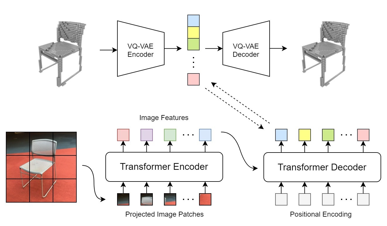
Figure 4: 3D-RETR with VQ-VAE. This corresponds to Setup 4 of our ablation study.

Appendix B Additional Examples

We show more examples of the ShapeNet dataset and the Pix3D dataset from our 3D-RETR-B model. Table 8 shows additional examples of the Pix3D dataset. Table 9 shows examples from the ShapeNet dataset with different numbers of views as inputs. We can see a clear quality improvement when more views become available.

Input
Prediction
GT

Table 8: Examples from the Pix3D dataset. All predictions are generated by 3D-RETR-B.

Input
1 view
2 views
3 views
4 views
5 views
8 views
12 views
16 views
20 views
GT

Table 9: Examples from the ShapeNet dataset. All predictions are generated by 3D-RETR-B.

Appendix C Model Performance with Different Views

In Table 2 of the paper, we show that 3D-RETR trained on three views still outperforms previous state-of-the-art results even when evaluated under different numbers of input views. In Table 10 and Figure 5, we give additional results on training and evaluating under different numbers of views. We can observe that more views during evaluation can boost model performance. Another observation is that models trained with more views are not necessarily better than models trained with fewer views, especially when the number of views available during evaluation is far fewer than the number of available views during training. For example, when only one view is available, the model trained with one view reaches an IoU of 0.680, while the model trained with 20 views only reaches an IoU of 0.534.

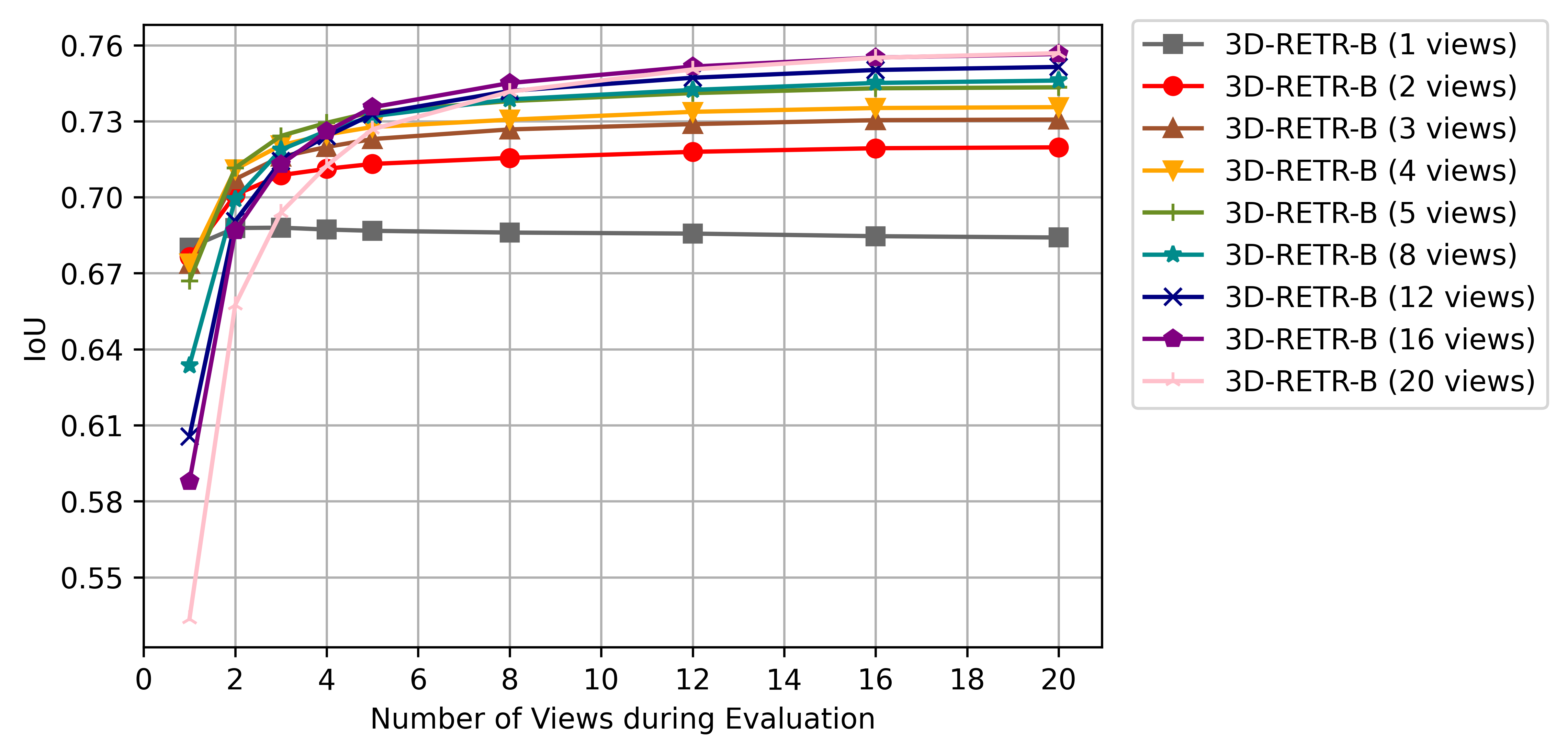
Figure 5: Models performance with different views.

	1 view	2 views	3 views	4 views	5 views	8 views	12 views	16 views	20 views
1 view	0.680	0.688	0.688	0.687	0.687	0.686	0.686	0.685	0.684
2 views	0.676	0.701	0.709	0.711	0.713	0.716	0.718	0.719	0.720
3 views	0.674	0.707	0.716	0.720	0.723	0.729	0.729	0.730	0.731
4 views	0.674	0.711	0.721	0.725	0.728	0.731	0.734	0.735	0.736
5 views	0.667	0.712	0.724	0.729	0.734	0.738	0.741	0.743	0.743
8 views	0.634	0.699	0.719	0.726	0.732	0.739	0.742	0.745	0.746
12 views	0.606	0.691	0.714	0.724	0.733	0.742	0.747	0.750	0.751
16 views	0.588	0.687	0.713	0.726	0.735	0.745	0.752	0.755	0.757
20 views	0.534	0.657	0.694	0.712	0.727	0.742	0.750	0.755	0.757

Table 10: Model performance with different views during training and evaluation. Bold indicates the best performance in an evaluation setting.

References

- [Agarwal et al.(2009)Agarwal, Snavely, Simon, Seitz, and Szeliski] Sameer Agarwal, Noah Snavely, Ian Simon, Steven M. Seitz, and Richard Szeliski. Building rome in a day. In ICCV, 2009.
- [Avetisyan et al.(2019)Avetisyan, Dahnert, Dai, Savva, Chang, and Nießner] Armen Avetisyan, Manuel Dahnert, Angela Dai, Manolis Savva, Angel X Chang, and Matthias Nießner. Scan2cad: Learning cad model alignment in rgb-d scans. In CVPR, 2019.
- [Berman et al.(2018)Berman, Triki, and Blaschko] M. Berman, A. Triki, and Matthew B. Blaschko. The lovasz-softmax loss: A tractable surrogate for the optimization of the intersection-over-union measure in neural networks. CVPR, 2018.
- [Bhat and Nayar(1998)] Dinkar N Bhat and Shree K Nayar. Ordinal measures for image correspondence. TPAMI, 1998.
- [Carion et al.(2020)Carion, Massa, Synnaeve, Usunier, Kirillov, and Zagoruyko] Nicolas Carion, Francisco Massa, Gabriel Synnaeve, Nicolas Usunier, Alexander Kirillov, and Sergey Zagoruyko. End-to-end object detection with transformers. In ECCV, 2020.
- [Chang et al.(2015)Chang, Funkhouser, Guibas, Hanrahan, Huang, Li, Savarese, Savva, Song, Su, Xiao, Yi, and Yu] Angel X. Chang, Thomas A. Funkhouser, Leonidas J. Guibas, Pat Hanrahan, Qi-Xing Huang, Zimo Li, Silvio Savarese, Manolis Savva, Shuran Song, Hao Su, Jianxiong Xiao, Li Yi, and Fisher Yu. Shapenet: An information-rich 3d model repository. CoRR, abs/1512.03012, 2015.
- [Chen and Zhang(2019)] Zhiqin Chen and Hao Zhang. Learning implicit fields for generative shape modeling. CVPR, 2019.
- [Cheng et al.(2014)Cheng, Leng, Wu, Cui, and Lu] Jian Cheng, Cong Leng, Jiaxiang Wu, Hainan Cui, and Hanqing Lu. Fast and accurate image matching with cascade hashing for 3d reconstruction. In CVPR, 2014.
- [Choromanski et al.(2021)Choromanski, Likhosherstov, Dohan, Song, Gane, Sarlós, Hawkins, Davis, Mohiuddin, Kaiser, Belanger, Colwell, and Weller] Krzysztof Marcin Choromanski, Valerii Likhosherstov, David Dohan, Xingyou Song, Andreea Gane, Tamás Sarlós, Peter Hawkins, Jared Quincy Davis, Afroz Mohiuddin, Lukasz Kaiser, David Benjamin Belanger, Lucy J. Colwell, and Adrian Weller. Rethinking attention with performers. In ICLR, 2021.
- [Choy et al.(2016)Choy, Xu, Gwak, Chen, and Savarese] Christopher B Choy, Danfei Xu, JunYoung Gwak, Kevin Chen, and Silvio Savarese. 3d-r2n2: A unified approach for single and multi-view 3d object reconstruction. In ECCV, 2016.
- [Dissanayake et al.(2001)Dissanayake, Newman, Clark, Durrant-Whyte, and Csorba] MWM Gamini Dissanayake, Paul Newman, Steve Clark, Hugh F Durrant-Whyte, and Michael Csorba. A solution to the simultaneous localization and map building (slam) problem. IEEE Transactions on robotics and automation, 2001.
- [Dosovitskiy et al.(2021)Dosovitskiy, Beyer, Kolesnikov, Weissenborn, Zhai, Unterthiner, Dehghani, Minderer, Heigold, Gelly, Uszkoreit, and Houlsby] Alexey Dosovitskiy, Lucas Beyer, Alexander Kolesnikov, Dirk Weissenborn, Xiaohua Zhai, Thomas Unterthiner, Mostafa Dehghani, Matthias Minderer, Georg Heigold, Sylvain Gelly, Jakob Uszkoreit, and Neil Houlsby. An image is worth 16x16 words: Transformers for image recognition at scale. In ICLR, 2021.
- [Esser et al.(2021)Esser, Rombach, and Ommer] Patrick Esser, Robin Rombach, and Björn Ommer. Taming transformers for high-resolution image synthesis. In CVPR, 2021.
- [Geiger et al.(2011)Geiger, Ziegler, and Stiller] Andreas Geiger, Julius Ziegler, and Christoph Stiller. Stereoscan: Dense 3d reconstruction in real-time. In IEEE intelligent vehicles symposium, 2011.
- [Groueix et al.(2018)Groueix, Fisher, Kim, Russell, and Aubry] Thibault Groueix, Matthew Fisher, Vladimir G. Kim, Bryan Russell, and Mathieu Aubry. AtlasNet: A Papier-Mâché Approach to Learning 3D Surface Generation. In CVPR, 2018.
- [Han et al.(2019)Han, Laga, and Bennamoun] Xianfeng Han, Hamid Laga, and Mohammed Bennamoun. Image-based 3d object reconstruction: State-of-the-art and trends in the deep learning era. TPAMI, 2019.
- [He et al.(2016)He, Zhang, Ren, and Sun] Kaiming He, X. Zhang, Shaoqing Ren, and Jian Sun. Deep residual learning for image recognition. CVPR, 2016.
- [Hermoza and Sipiran(2018)] Renato Hermoza and Ivan Sipiran. 3d reconstruction of incomplete archaeological objects using a generative adversarial network. In CGI, 2018.
- [Izadi et al.(2011)Izadi, Kim, Hilliges, Molyneaux, Newcombe, Kohli, Shotton, Hodges, Freeman, Davison, et al.] Shahram Izadi, David Kim, Otmar Hilliges, David Molyneaux, Richard Newcombe, Pushmeet Kohli, Jamie Shotton, Steve Hodges, Dustin Freeman, Andrew Davison, et al. Kinectfusion: real-time 3d reconstruction and interaction using a moving depth camera. In UIST, 2011.
- [Jiang et al.(2018)Jiang, Shi, Qi, and Jia] Li Jiang, Shaoshuai Shi, Xiaojuan Qi, and Jiaya Jia. Gal: Geometric adversarial loss for single-view 3d-object reconstruction. In ECCV, 2018.
- [Kar et al.(2017)Kar, Häne, and Malik] Abhishek Kar, Christian Häne, and Jitendra Malik. Learning a multi-view stereo machine. In NeurIPS, 2017.
- [Kitaev et al.(2020)Kitaev, Kaiser, and Levskaya] Nikita Kitaev, Lukasz Kaiser, and Anselm Levskaya. Reformer: The efficient transformer. In ICLR, 2020.
- [Lin et al.(2020)Lin, Goyal, Girshick, He, and Dollár] Tsung-Yi Lin, Priya Goyal, Ross B. Girshick, Kaiming He, and Piotr Dollár. Focal loss for dense object detection. TPAMI, 2020.
- [Liu et al.(2021)Liu, Lin, Cao, Hu, Wei, Zhang, Lin, and Guo] Ze Liu, Yutong Lin, Yue Cao, Han Hu, Yixuan Wei, Zheng Zhang, Stephen Lin, and Baining Guo. Swin transformer: Hierarchical vision transformer using shifted windows. ICCV, 2021.
- [Loshchilov and Hutter(2019)] Ilya Loshchilov and F. Hutter. Decoupled weight decay regularization. In ICLR, 2019.
- [Lowe(2004)] David G Lowe. Distinctive image features from scale-invariant keypoints. IJCV, 2004.
- [Mandikal et al.(2018)Mandikal, L., Agarwal, and Radhakrishnan] Priyanka Mandikal, Navaneet K. L., Mayank Agarwal, and Venkatesh Babu Radhakrishnan. 3d-lmnet: Latent embedding matching for accurate and diverse 3d point cloud reconstruction from a single image. In BMVC, 2018.
- [Mescheder et al.(2019)Mescheder, Oechsle, Niemeyer, Nowozin, and Geiger] Lars M. Mescheder, Michael Oechsle, Michael Niemeyer, S. Nowozin, and Andreas Geiger. Occupancy networks: Learning 3d reconstruction in function space. CVPR, 2019.
- [Mildenhall et al.(2020)Mildenhall, Srinivasan, Tancik, Barron, Ramamoorthi, and Ng] Ben Mildenhall, Pratul P. Srinivasan, Matthew Tancik, Jonathan T. Barron, Ravi Ramamoorthi, and Ren Ng. Nerf: Representing scenes as neural radiance fields for view synthesis. In ECCV, 2020.
- [Niemeyer et al.(2020)Niemeyer, Mescheder, Oechsle, and Geiger] Michael Niemeyer, Lars Mescheder, Michael Oechsle, and Andreas Geiger. Differentiable volumetric rendering: Learning implicit 3d representations without 3d supervision. In Proceedings IEEE Conf. on Computer Vision and Pattern Recognition (CVPR), 2020.
- [Popa et al.(2017)Popa, Zanfir, and Sminchisescu] Alin-Ionut Popa, Mihai Zanfir, and Cristian Sminchisescu. Deep multitask architecture for integrated 2d and 3d human sensing. In CVPR, 2017.
- [Ramesh et al.(2021)Ramesh, Pavlov, Goh, Gray, Voss, Radford, Chen, and Sutskever] Aditya Ramesh, Mikhail Pavlov, Gabriel Goh, Scott Gray, Chelsea Voss, Alec Radford, Mark Chen, and Ilya Sutskever. Zero-shot text-to-image generation. In Marina Meila and Tong Zhang, editors, ICML, 2021.
- [Richter and Roth(2018)] Stephan R. Richter and S. Roth. Matryoshka networks: Predicting 3d geometry via nested shape layers. CVPR, 2018.
- [Saponaro et al.(2014)Saponaro, Sorensen, Rhein, Mahoney, and Kambhamettu] Philip Saponaro, Scott Sorensen, Stephen Rhein, Andrew R Mahoney, and Chandra Kambhamettu. Reconstruction of textureless regions using structure from motion and image-based interpolation. In ICIP, 2014.
- [Sitzmann et al.(2019)Sitzmann, Zollhöfer, and Wetzstein] Vincent Sitzmann, Michael Zollhöfer, and Gordon Wetzstein. Scene representation networks: Continuous 3d-structure-aware neural scene representations. In Advances in Neural Information Processing Systems, 2019.
- [Soltani et al.(2017)Soltani, Huang, Wu, Kulkarni, and Tenenbaum] Amir Arsalan Soltani, Haibin Huang, Jiajun Wu, Tejas D. Kulkarni, and Joshua B. Tenenbaum. Synthesizing 3d shapes via modeling multi-view depth maps and silhouettes with deep generative networks. In CVPR, 2017.
- [Su et al.(2015)Su, Qi, Li, and Guibas] Hao Su, C. Qi, Yangyan Li, and L. Guibas. Render for cnn: Viewpoint estimation in images using cnns trained with rendered 3d model views. ICCV, 2015.
- [Sudre et al.(2017)Sudre, Li, Vercauteren, Ourselin, and Cardoso] C. Sudre, Wenqi Li, Tom Kamiel Magda Vercauteren, S. Ourselin, and M. Jorge Cardoso. Generalised dice overlap as a deep learning loss function for highly unbalanced segmentations. DLMIA, 2017.
- [Sun et al.(2018)Sun, Wu, Zhang, Zhang, Zhang, Xue, Tenenbaum, and Freeman] Xingyuan Sun, Jiajun Wu, Xiuming Zhang, Zhoutong Zhang, Chengkai Zhang, Tianfan Xue, J. Tenenbaum, and W. Freeman. Pix3d: Dataset and methods for single-image 3d shape modeling. CVPR, 2018.
- [Tatarchenko et al.(2017)Tatarchenko, Dosovitskiy, and Brox] M. Tatarchenko, A. Dosovitskiy, and T. Brox. Octree generating networks: Efficient convolutional architectures for high-resolution 3d outputs. In ICCV, 2017.
- [Touvron et al.(2021)Touvron, Cord, Douze, Massa, Sablayrolles, and Jégou] Hugo Touvron, Matthieu Cord, Matthijs Douze, Francisco Massa, Alexandre Sablayrolles, and Hervé Jégou. Training data-efficient image transformers & distillation through attention. In Marina Meila and Tong Zhang, editors, ICML, 2021.
- [Tulsiani et al.(2017a)Tulsiani, Zhou, Efros, and Malik] Shubham Tulsiani, Tinghui Zhou, Alexei A. Efros, and Jitendra Malik. Multi-view supervision for single-view reconstruction via differentiable ray consistency. In CVPR, 2017a.
- [Tulsiani et al.(2017b)Tulsiani, Zhou, Efros, and Malik] Shubham Tulsiani, Tinghui Zhou, Alexei A Efros, and Jitendra Malik. Multi-view supervision for single-view reconstruction via differentiable ray consistency. In CVPR, 2017b.
- [Tulsiani et al.(2018)Tulsiani, Efros, and Malik] Shubham Tulsiani, Alexei A Efros, and Jitendra Malik. Multi-view consistency as supervisory signal for learning shape and pose prediction. In CVPR, 2018.
- [van den Oord et al.(2017)van den Oord, Vinyals, and Kavukcuoglu] Aäron van den Oord, Oriol Vinyals, and K. Kavukcuoglu. Neural discrete representation learning. In NeurIPS, 2017.
- [Vaswani et al.(2017)Vaswani, Shazeer, Parmar, Uszkoreit, Jones, Gomez, Kaiser, and Polosukhin] Ashish Vaswani, Noam Shazeer, Niki Parmar, Jakob Uszkoreit, Llion Jones, Aidan N. Gomez, Lukasz Kaiser, and Illia Polosukhin. Attention is all you need. In NeurIPS, 2017.
- [Wang et al.(2018)Wang, Zhang, Li, Fu, Liu, and Jiang] Nanyang Wang, Yinda Zhang, Zhuwen Li, Yanwei Fu, W. Liu, and Yu-Gang Jiang. Pixel2mesh: Generating 3d mesh models from single rgb images. In ECCV, 2018.
- [Wang et al.(2021)Wang, Xu, Wang, Shen, Cheng, Shen, and Xia] Yuqing Wang, Zhaoliang Xu, Xinlong Wang, Chunhua Shen, Baoshan Cheng, Hao Shen, and Huaxia Xia. End-to-end video instance segmentation with transformers. In CVPR, 2021.
- [Xie et al.(2019)Xie, Yao, Sun, Zhou, and Zhang] Haozhe Xie, Hongxun Yao, Xiaoshuai Sun, Shangchen Zhou, and Shengping Zhang. Pix2vox: Context-aware 3d reconstruction from single and multi-view images. In CVPR, 2019.
- [Xie et al.(2020)Xie, Yao, Zhang, Zhou, and Sun] Haozhe Xie, Hongxun Yao, Shengping Zhang, Shangchen Zhou, and Wenxiu Sun. Pix2vox++: Multi-scale context-aware 3d object reconstruction from single and multiple images. IJCV, 2020.
- [Yang et al.(2019)Yang, Wang, Markham, and Trigoni] Bo Yang, Sen Wang, A. Markham, and Niki Trigoni. Robust attentional aggregation of deep feature sets for multi-view 3d reconstruction. IJCV, 2019.
- [Yang et al.(2020)Yang, Yang, Fu, Lu, and Guo] Fuzhi Yang, Huan Yang, Jianlong Fu, Hongtao Lu, and Baining Guo. Learning texture transformer network for image super-resolution. In CVPR, 2020.
- [Yariv et al.(2020)Yariv, Kasten, Moran, Galun, Atzmon, Ronen, and Lipman] Lior Yariv, Yoni Kasten, Dror Moran, Meirav Galun, Matan Atzmon, Basri Ronen, and Yaron Lipman. Multiview neural surface reconstruction by disentangling geometry and appearance. NeurIPS, 2020.