Provable RL with Exogenous Distractors via Multistep Inverse Dynamics

Provable RL with Exogenous Distractors via Multistep Inverse Dynamics

Abstract

Many real-world applications of reinforcement learning (RL) require the agent to deal with high-dimensional observations such as those generated from a megapixel camera. Prior work has addressed such problems with representation learning, through which the agent can provably extract endogenous, latent state information from raw observations and subsequently plan efficiently. However, such approaches can fail in the presence of temporally correlated noise in the observations, a phenomenon that is common in practice. We initiate the formal study of latent state discovery in the presence of such exogenous noise sources by proposing a new model, the Exogenous Block MDP (EX-BMDP), for rich observation RL. We start by establishing several negative results, by highlighting failure cases of prior representation learning based approaches. Then, we introduce the Predictive Path Elimination (${\tt PPE}$) algorithm, that learns a generalization of inverse dynamics and is provably sample and computationally efficient in EX-BMDPs when the endogenous state dynamics are near deterministic. The sample complexity of ${\tt PPE}$ depends polynomially on the size of the latent endogenous state space while not directly depending on the size of the observation space, nor the exogenous state space. We provide experiments on challenging exploration problems which show that our approach works empirically.

1 Introduction

In many real-world applications such as robotics there can be large disparities in the size of agent’s observation space (for example, the image generated by agent’s camera), and a much smaller latent state space (for example, the agent’s location and orientation) governing the rewards and dynamics. This size disparity offers an opportunity: how can we construct reinforcement learning (RL) algorithms which can learn an optimal policy using samples that scale with the size of the latent state space rather than the size of the observation space? Several families of approaches have been proposed based on solving various ancillary prediction problems including autoencoding [28, 16], inverse modeling [24, 6], and contrastive learning [20] based approaches. These works have generated some significant empirical successes, but are there provable (and hence more reliable) foundations for their success? More generally, what are the right principles for learning with latent state spaces?

In real-world applications, a key issue is robustness to noise in the observation space. When noise comes from the observation process itself, such as due to measurement error, several approaches have been recently developed to either explicitly identify [11, 21, 2] or implicitly leverage [17] the presence of latent state structure for provably sample-efficient RL. However, in many real-world scenarios, the observations consist of many elements (e.g. weather, lighting conditions, etc.) with temporally correlated dynamics (see e.g. Figure 1 and the example below) that are entirely independent of the agent’s actions and rewards. The temporal dynamics of these elements precludes us from treating them as uncorrelated noise, and as such, most previous approaches resort to modeling their dynamics. However, this is clearly wasteful as these elements have no bearing on the RL problem being solved.

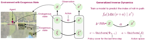
Figure 1: Left: Shows an example where an agent is walking next to a pond in a park and observes the world as an image ($x$). The world consists of a latent endogenous state, containing variable such as agent’s position, and a much larger latent exogenous state containing variables such as motion of ducks, changes in sunlight, ripples in the water, etc. Center: The novel exogenous block MDP setting introduced here. The exogenous state is unaffected by agent’s action. Right: We show that ${\tt PPE}$ learns a generalized form of inverse dynamics that is able to recover the endogenous state.

As an example, consider the setting in Figure 1. An agent is walking in a park on a lonely sidewalk next to a pond. The agent’s observation space is the image generated by its camera, the latent endogenous state is its position on the sidewalk, and the exogenous noise is provided by motion of ducks or people in the background, swaying of trees and changes in lighting conditions, typically unaffected by the agent’s actions. While there is a line of recent empirical work that aims to remove causally irrelevant aspects of the observation [13, 29], theoretical treatment is quite limited [10] and no prior works address sample-efficient learning with provable guarantees. Given this, the key question here is:

How can we learn using an amount of data scaling with just the size of the endogenous latent state, while ignoring the temporally correlated exogenous observation noise?

We initiate a formal treatment of RL settings where the learner’s observations are jointly generated by a latent endogenous state and an uncontrolled exogenous state, which is unaffected by the agent’s actions and does not affect the agent’s task. We study a subset of such problems called Exogenous Block MDPs (EX-BMDPs), where the endogenous state is discrete and decodable from the observations. We first highlight the challenges in solving EX-BMDPs by illustrating the failures of many prior representation learning approaches [24, 21, 17, 2, 29]. These failure happen either due to creating too many latent states, such as one for each combination of ducks and passers-by in the example above leading to sample inefficiency in exploration, or due to lack of exhaustive exploration.

We identify one recent approach developed by Du et al. [11] with favorable properties for a class of EX-BMDPs with near-deterministic latent state dynamics. In Section 4 and Section 5, we develop a variation of their algorithm and analyze its performance for near-deterministic EX-BMDPs. The algorithm, called Path Prediction and Elimination (${\tt PPE}$), learns a form of multi-step inverse dynamics by predicting the identity of the path that generates an observation. For near-deterministic EX-BMDPs, we prove that ${\tt PPE}$ successfully explores the environment using $O((SA)^{2}H\log(|\mathcal{F}|/\delta))$ samples where $S$ is the size of the latent endogenous state space, $A$ is the number of actions, $H$ is the horizon and $\mathcal{F}$ is a function class employed to solve a maximum likelihood problem of inferring the path which generated an observation. Several prior works [15, 23] have also considered a multi-step inverse dynamics approach to learn a near optimal policy. However, these works do not consider the EX-BMDP model. Further, it is unknown whether these algorithms have guarantees for EX-BMDP similar to what we present for ${\tt PPE}$. Theoretical analysis of the performance of these algorithms in the presence of exogenous noise is an interesting future work direction.

Empirically, in Section 6, we demonstrate the performance of ${\tt PPE}$ and various prior baselines in a challenging exploration problem with exogenous noise. We show that baselines fail to decode the endogenous state and either end up over-abstracting (creating an abstract state which aliases essentially-different states) or under-abstracting (creating essentially the same clones of states). We further, show that ${\tt PPE}$ is able to recover the latent endogenous model in a visually complex navigation problem, in accordance with the theory.

2 Exogenous Block MDP Setting

We introduce a novel Exogenous Block Markov Decision Process (EX-BMDP) setting to model environments with exogenous noise. We briefly describe notations before presenting a formal treatment of EX-BMDP.

Notations.

For a given set $\mathcal{U}$, we use $\Delta(\mathcal{U})$ to denote the set of all probability distributions over $\mathcal{U}$. For a given natural number $N\in\mathbb{N}$, we use the notation $[N]$ to denote the set $\{1,2,\cdots,N\}$. Lastly, for a probability distribution $p\in\Delta(\mathcal{U})$, we define its support as $supp~{}p=\{u\mid p(u)>0,u\in\mathcal{U}\}$.

We start with describing the Block Markov Decision Process (BMDP) [11]. This process consists of a finite set of observations $\mathcal{X}$, a set of latent states $\mathcal{Z}$ with cardinality $Z$, a finite set of actions $\mathcal{A}$ with cardinality $A$, a transition function $T:\mathcal{Z}\times\mathcal{A}\rightarrow\Delta(\mathcal{Z})$, an emission function $q:\mathcal{Z}\times\mathcal{A}\rightarrow\Delta(\mathcal{X})$, a reward function $R:\mathcal{X}\times\mathcal{A}\rightarrow[0,1]$, a horizon $H\in\mathbb{N}$, and a start state distribution $\mu\in\Delta(\mathcal{Z})$. The agent interacts with the environment by repeatedly generating $H$-step trajectories $(z_{1},x_{1},a_{1},r_{1},\cdots,z_{H},x_{H},a_{H},r_{H})$ where $z_{1}\sim\mu(\cdot)$ and for every $h\in[H]$ we have $x_{h}\sim q(\cdot\mid z_{h})$, $r_{h}=R(x_{h},a_{h})$, and if $h<H$, then $z_{h+1}\sim T(\cdot\mid z_{h},a_{h})$. The agent does not observe the states $\left(z_{1},\cdots,z_{H}\right)$, instead receiving only the observations $\left(x_{1},\cdots,x_{H}\right)$ and rewards $\left(r_{1},\cdots,r_{H}\right)$. We assume that the emission distributions of any two latent states are disjoint, usually referred as the block assumption: $supp(q(\cdot\mid z_{1}))\cap supp(q(\cdot|z_{2}))=\emptyset\text{ when $z_{1}\neq z_{2}.$}$ The agent chooses actions using a policy $\pi:\mathcal{X}\rightarrow\Delta(\mathcal{A})$. We also define the set of non-stationary policies $\Pi_{\textrm{NS}}=\Pi^{H}$ as a $H$-length tuple, with $(\pi_{1},\cdots,\pi_{H})\in\Pi_{\textrm{NS}}$ denoting that the action at time step $h$ is taken as $a_{h}\sim\pi_{h}(\cdot\mid x_{h})$. The value $V(\pi)$ of a policy $\pi$ is the expected episodic sum of rewards $V(\pi):=\mathbb{E}_{\pi}[\sum_{h=1}^{H}R(x_{h},a_{h})]$. The optimal policy is given by $\pi^{\star}=\arg\max_{\pi\in\Pi_{\textrm{NS}}}V(\pi)$. We denote by $\mathbb{P}_{h}(x|\pi)$ the probability distribution over observations $x$ at time step $h$ when following a policy $\pi$. Lastly, we refer to an open loop policy as an element in all $\mathcal{A}^{H}$ sequences of actions. An open loop policy follows a pre-determined sequence of actions $\left\{a_{1},..,a_{H}\right\}$ for $H$ time steps, unaffected by state information.

Given the aforementioned definitions, we define an EX-BMDP as follows:

Definition 1 (Exogenous Block Markov Decision Processes).

An EX-BMDP is a BMDP such that the latent state can be decoupled into two parts $z=(s,\xi)$ where $s\in\mathcal{S}$ is the endogenous state and $\xi\in\Xi$ is the exogenous state. For $z\in\mathcal{Z}$ the initial distribution and transition functions are decoupled, that is: $\mu(z)=\mu(s)\mu_{\xi}(\xi)$, and $T(z^{\prime}\mid z,a)=T(s^{\prime}\mid s,a)T_{\xi}(\xi^{\prime}\mid\xi).$

The observation space $\mathcal{X}$ can be arbitrarily large to model which could be a high-dimensional real vector denoting an image, sound, or haptic data in an EX-BMDP. The endogenous state $s$ captures the information that can be manipulated by the agent. Figure 1, center, visualizes the transition dynamics factorization. We assume that the set of all endogenous states $\mathcal{S}$ is finite with cardinality $S$. The exogenous state $\xi$ captures all the other information that the agent cannot control and does not affect the information it can manipulate. Again, we make no assumptions on the exogenous dynamics nor on its cardinality $|\Xi|$ which may be arbitrarily large. We note that the block assumption of the EX-BMDP implies the existence of two inverse mappings: $\phi^{\star}:\mathcal{X}\rightarrow\mathcal{S}$ to map an observation to its endogenous state, and $\phi^{\star}_{\xi}:\mathcal{X}\rightarrow\Xi$ to map it to its exogenous state.

Justification of assumptions.

The block assumption has been made by prior work (e.g., [11], [29]) to model many real-world settings where the observation is rich, i.e., it contains enough information to decode the latent state. The decoupled dynamics assumption made in the EX-BMDP setting is a natural way to characterize exogenous noise; the type of noise that is not affected by our actions nor affects the endogenous state but may have non-trivial dynamic. This decoupling captures the movement of ducks, captured in the visual field of the agent in Figure 1, and many additional exogenous processes (e.g., movement of clouds in a navigation task).

Goal.

Our formal objective is reward-free learning. We wish to find a set of policies, we call a policy cover, that can be used to explore the entire state space. Given a policy cover, and for any reward function, we can find a near optimal policy by applying dynamic programming (e.g., [5]), policy optimization (e.g., [18, 3, 27]) or value (e.g., [4]) based methods.

Definition 2 ($\alpha$-policy cover).

Let $\Psi_{h}$ be a finite set of non-stationary policies. We say $\Psi_{h}$ is an $\alpha$-policy cover for the $h^{th}$ time step if for all $z\in\mathcal{Z}$ it holds that ${\max_{\pi\in\Psi_{h}}\mathbb{P}_{h}(z|\pi)\geq\max_{\pi\in\Pi_{NS}}\mathbb{P}_{h}(z|\pi)-\alpha.}$ If $\alpha=0$ we call $\Psi_{h}$ a policy cover.

For standard BMDPs the policy cover is simply the set of policies that reaches each latent state of the BMDP [11, 21, 2]. Thus, for a BMDP, the cardinality of the policy cover scales with $\left|\mathcal{Z}\right|$. The structure of EX-BMDPs allows to reduce the size of the policy cover significantly to $\left|{\mathcal{S}}\right|\ll\left|\mathcal{Z}\right|=\left|{\mathcal{S}}\right|\left|\Xi\right|$ when the size of the exogenous state space is large. Specifically, we show that the set of policies that reach each endogenous state, and do not depend on the exogenous part of the state is also a policy cover (see Appendix B, Proposition 4). Further, the proposed algorithm ${\tt PPE}$, learns such a policy cover and requires number of samples that depends polynomially on $|{\mathcal{S}}|$ instead of $|\mathcal{Z}|$ or $|\mathcal{X}|$.

3 Failures of Prior Approaches

We now describe the limitation of prior RL approaches in the presence of exogenous noise. We provide an intuitive analysis over here, and defer a formal statement and proof to Appendix A.

Limitation of Noise-Contrastive learning.

Noise-contrastive learning has been used in RL to learn a state abstraction by exploiting temporal information. Specifically, the Homer algorithm [21] trains a model to distinguish between real and imposter transitions. This is done by collecting a dataset of quads $(x,a,x^{\prime},y)$ where $y=1$ means the transition was $(x,a,x^{\prime})$ was observed and $y=0$ means that $(x,a,x^{\prime})$ was not observed. Homer then trains a model $p_{\theta}(y\mid x,a,\phi_{\theta}(x^{\prime}))$ with parameters $\theta$, on the dataset, by predicting whether a given pair of transition was observed or not. This provides a state abstraction $\phi_{\theta}:\mathcal{X}\rightarrow\mathbb{N}$ for exploring the environment. Homer can provably solve Block MDPs. Unfortunately, in the presence of exogenous noise, Homer distinguishes between two transitions that represent transition between the same latent endogenous states but different exogenous states. In our walk in the park example, even if the agent moves between same points in two transitions, the model maybe able to tell these transitions apart by looking at the position of ducks which may have different behaviour in the two transitions. This results in the Homer creating $\mathcal{O}(|\mathcal{Z}|)$ many abstract states. We call this the under-abstraction problem.

Limitation of Inverse Dynamics.

Another common approach in empirical works is based on modeling the inverse dynamics of the system, such as the ICM module of Pathak et al. [24]. In such approaches, we learn a representation by using consecutive observations to predict the action that was taken between them. Such a representation can ignore all information that is not relevant for action prediction, which includes all exogenous/uncontrollable information. However, it can also ignore controllable information. This may result in a failure to sufficiently explore the environment. In this sense, inverse dynamics approaches result in an over-abstraction problem where observations from different endogenous states can be mapped to the same abstract state. The over-abstraction problem was described at [21], when the starting state is random. In Appendix A.3 we show inverse dynamics may over-abstract when the initial starting state is deterministic.

Limitation of Bisimulation.

[29] proposed learning a bisimulation metric to learn a representation which is invariant to exogenous noise. Unfortunately, it is known that bisimulation metric cannot be learned in a sample-efficient manner (Modi et al. [22], Proposition B.1). Intuitively, when the reward is same everywhere, then bisimulation merges all states into a single abstract state. This creates exploration issue in sparse reward settings, since the agent can merge all states into a single abstract state until it receives a non-trivial reward. Hence, the learned abstract states provide no help in exploring the environment.

Bellman rank might depend on $|\Xi|$.

The Bellman rank was introduced in [17] as a complexity measure for the learnability of an RL problem with function approximations. To date, most of the learnable RL problems have a small Bellman rank. However, we show in Appendix A that Bellman rank for EX-BMDP can scale as $\mathcal{O}(|\Xi|)$. This shows that EX-BMDP is a highly non-trivial setting as we don’t even have sample-efficient algorithms that can solve it without being computationally-efficient.

In Appendix A we also describe the failures of ${\tt FLAMBE}$ [2]) and autoencoding based approaches [28].

4 Reinforcement Learning for EX-BMDPs

Algorithm 1 ${\tt PPE}(\delta,\eta)$: Predictive Path Elimination

1:Set $\Psi_{1}=\{\bot\}$, stochasticity level $\eta\leq\frac{1}{4SH}$ //$\bot$ denotes an empty path

2:for $h=2,\ldots,H$ do

3:     Set $N=16\left(|\Psi_{h-1}\circ A|\right)^{2}\log\left(\frac{|\mathcal{F}||\Psi_{h-1}|AH}{\delta}\right)$

4:     Collect a dataset $\mathcal{D}$ of $N$ i.i.d. tuples $(x,\upsilon)$ where $\upsilon\sim{\tt Unf}(\Psi_{h-1}\circ\mathcal{A})$ and $x\sim\mathbb{P}(x_{h}\mid\upsilon)$.

5:     Solve multi-class classification problem: $\hat{f}_{h}=\arg\max_{f\in\mathcal{F}}\sum_{(x,\upsilon)\in\mathcal{D}}\ln f(\textrm{idx}(\upsilon)\mid x)$.

6:     for $1\leq i<j\leq|\Psi_{h-1}\circ\mathcal{A}|$ do

7:         Calculate the path prediction gap: $\widehat{\Delta}(i,j)=\frac{1}{N}\sum_{(x,\upsilon)\in\mathcal{D}}\left|\hat{f}_{h}(i|x)-\hat{f}_{h}(j|x)\right|.$

8:         If $\widehat{\Delta}(i,j)\leq\frac{5/8}{|\Psi_{h-1}\circ\mathcal{A}|}$, then eliminate path $\upsilon$ with $\mathrm{idx}(\upsilon)=j$. //$\upsilon_{i}$ and $\upsilon_{j}$ visit the same state      

9:     $\Psi_{h}$ is defined as the set of all paths in $\Psi_{h-1}\circ\mathcal{A}$ that have not been eliminated in line 8.

In this section, we present an algorithm Predictive Path Elimination (${\tt PPE}$) that we later show can provably solve any EX-BMDP with nearly deterministic dynamics and start state distribution of the endogenous state, while making no assumptions on the dynamics or start state distribution of the exogenous state (Algorithm 1). Before describing ${\tt PPE}$, we highlight that ${\tt PPE}$ can be thought of as a computationally-efficient and simpler alternative to Algorithm 4 of [11] who studied rich-observation setting without exogenous noise. Due to the apparent difference of the algorithms we keep the presentation of our algorithm fully self-contained.

${\tt PPE}$ performs iterations over the time steps $h\in\{2,\cdots,H\}$. In the $h^{th}$ iteration, it learns a policy cover $\Psi_{h}$ for time step $h$ containing open-loop policies. This is done by first augmenting the policy cover for previous time step by one step. Formally, we define $\Upsilon_{h}=\Psi_{h-1}\circ\mathcal{A}=\{\pi\circ a\mid\pi\in\Psi_{h-1},a\in\mathcal{A}\}$ where $\pi\circ a$ is an open-loop policy that follows $\pi$ till time step $h-1$ and then takes action $a$. Since we assume the transition dynamics to be near-deterministic, therefore, we know that there exists a policy cover for time step $h$ that is a subset of $\Upsilon_{h}$ and whose size is equal to the number of reachable states at time step $h$. Further, as the transitions are near-deterministic, we refer to an open-loop policy as a path, as we can view the policy as tracing a path in the latent transition model. ${\tt PPE}$ works by eliminating paths in $\Upsilon_{h}$ so that we are left with just a single path for each reachable state. This is done by collecting a dataset $\mathcal{D}$ of tuples $(x,\upsilon)$ where $\upsilon$ is a uniformly sampled from $\Upsilon_{h}$ and $x\sim\mathbb{P}_{h}(x\mid\upsilon)$ (line 4). We train a classifier $\hat{f}_{h}$ using $\mathcal{D}$ by predicting the index $\textrm{idx}(\upsilon)$ of the path $\upsilon$ from the observation $x$ (line 5). Index of paths in $\Upsilon_{h}$ are computed with respect to $\Upsilon_{h}$ and remain fixed throughout training. Intuitively, if $\hat{f}_{h}(i\mid x)$ is sufficiently large, then we can hope that the path $\upsilon_{i}$ visits the state $\phi^{\star}(x)$. Further, we can view this prediction problem as learning a multistep inverse dynamics model since the open-loop policy contains information about all previous actions and not just the last action. For every pair of paths in $\Upsilon_{h}$, we first compute a path prediction gap $\widehat{\Delta}$(line 7). If the gap is too small, we show it implies that these paths reach the same endogenous state, hence we can eliminate a single redundant path from this pair (line 8). Finally, $\Psi_{h}$ is defined as the set of all paths in $\Upsilon_{h}$ which were not eliminated. ${\tt PPE}$ reduces RL to performing $H$ standard classification problems. Further, the algorithm is very simple and in practice requires just a single hyperparameter ($N$). We believe these properties will make it well-suited for many problems.

Recovering an endogenous state decoder.

We can recover a endogenous state decoder $\hat{\phi}_{h}$ for each time step $h\in\{2,3,\cdots,H\}$ directly from $\hat{f}_{h}$ as shown below:

$$\hat{\phi}_{h}(x)=\min\left\{i\mid\hat{f}_{h}(i\mid x)\geq\max_{j}\hat{f}_{h}(j\mid x)-\mathcal{O}(\nicefrac{{1}}{{|\Upsilon_{h}|}}),i\in\left[|\Upsilon_{h}|\right]\right\}.$$

Intuitively, this assigns the observation to the path with smallest index that has the highest chance of visiting $x$, and therefore, $\phi^{\star}(x)$. We are implicitly using the decoder for exploring, since we rely on using $\hat{f}_{h}$ for making planning decisions. We will evaluate the accuracy of this decoder in Section 6.

Recovering the latent transition dynamics.

${\tt PPE}$ can also be used to recover a latent endogenous transition dynamics. The direct way is to use the learned decoder $\hat{\phi}_{h}$ along with episodes collected by ${\tt PPE}$ during the course of training and do count-based estimation. However, for most problems, recovering an approximate deterministic transition dynamics suffices, which can be directly read from the path elimination data. We accomplish this by recovering a partition of paths in $\Psi_{h-1}\times\mathcal{A}$ where two paths in the same partition set are said to be merged with each other. In the beginning, each path is only merged with itself. When we eliminate a path $\upsilon_{j}$ on comparison with $\upsilon_{i}$ in line 8, then all paths currently merged with $\upsilon_{j}$ get merged with $\upsilon_{i}$. We then define an abstract state space $\widehat{{\mathcal{S}}}_{h}$ for time step $h$ that contains an abstract state $j$ for each path $\upsilon_{j}\in\Psi_{h}$. Further, we recover a latent deterministic transition dynamics for time step $h-1$ as $\hat{T}_{h-1}:\widehat{{\mathcal{S}}}_{h-1}\times\mathcal{A}\rightarrow\widehat{{\mathcal{S}}}_{h}$ where we set $\hat{T}_{h-1}(i,a)=j$ if the path $\upsilon_{j}\in\Psi_{h}$ gets merged with path $\upsilon^{\prime}_{i}\circ a\in\Psi_{h}$ where $\upsilon^{\prime}_{i}\in\Psi_{h-1}$.

Learning a near optimal policy given a policy cover.

${\tt PPE}$ runs in a reward-free setting. However, the recovered policy cover and dynamics can be directly used to optimize any given reward function with existing methods. If the reward function depends on the exogenous state then we can use the ${\tt PSDP}$ algorithm [5] to learn a near-optimal policy. ${\tt PSDP}$ is a model-free dynamic programming method that only requires policy cover as input (see Appendix D.1 for details). However, if the reward function only depends on the endogenous state, then we can use a computationally cheaper value-iteration algorithm ${\tt VI}$ that uses the policy cover and recovered transition dynamics. ${\tt VI}$ is a model-based algorithm that estimates the reward for each state and action, and performs dynamic programming on the model (see Appendix D.2 for details). In each case, the sample complexity of learning a near-optimal policy, given the output of the ${\tt PPE}$ algorithm, scales with the size of endogenous and not the exogenous state space or the size of observation space.

5 Theoretical Analysis and Discussion

We provide the main sample complexity guarantee for ${\tt PPE}$ as well as additional intuition for why it works. We analyze the algorithm in near-deterministic MDPs defined as follows: Two transition functions $T_{1}$ and $T_{2}$ are $\eta$-close if for all $h\in[H],a\in\mathcal{A},s\in{\mathcal{S}}_{h}$ it holds that $||T_{1}(\cdot\mid s,a)-T_{2}(\cdot\mid s,a)||_{1}\leq\eta$. Analogously, two starting distribution $\mu_{1}$ and $\mu_{2}$ are $\eta$-close if $||\mu_{1}(\cdot)-\mu_{2}(\cdot)||_{1}\leq\eta$. We emphasize that near-deterministic dynamics are common in real-world applications like robotics.

Assumption 1 (Near deterministic endogenous dynamics).

We assume the endogenous dynamics is $\eta$-close to a deterministic model $(\mu_{D,\eta},T_{D,\eta})$ where $\eta\leq 1/(4SH)$.

We make a realizability assumption for the regression problem solved by ${\tt PPE}$ (line 5). We assume that $\mathcal{F}$ is expressive enough to represent the Bayes optimal classifier of the regression problems created by ${\tt PPE}$.

Assumption 2 (Realizability).

For any $h\in[H]$, and any set of paths $\Upsilon\subseteq\mathcal{A}^{h}$ with $|\Upsilon|\leq SA$ and where $\mathcal{A}^{h}$ denotes the set of all paths of length $h$, there exists $f^{\star}_{\Upsilon,h}\in\mathcal{F}$ such that: $f^{\star}_{\Upsilon,h}({\tt idx}(\upsilon)\mid x)=\frac{\mathbb{P}_{h}(\phi^{\star}(x))\mid\upsilon)}{\sum_{\upsilon^{\prime}\in\Upsilon}\mathbb{P}_{h}(\phi^{\star}(x))\mid\upsilon^{\prime})},$ for all $\upsilon\in\Upsilon$ and $x\in\mathcal{X}$ with $\sum_{\upsilon^{\prime}\in\Upsilon}\mathbb{P}_{h}(\phi^{\star}(x))\mid\upsilon^{\prime})>0$.

In this assumption, the function $f^{\star}_{\Upsilon,h}(\upsilon\mid x)$ denotes the Bayes optimal classifier for the regression problem in the $h^{th}$ iteration when $\Upsilon_{h}=\Upsilon$. Realizability assumptions are common in theoretical analysis (e.g., [21], [2]). In practice, we use expressive neural networks to solve the regression problem, so we expect the realizability assumption to hold. Note that there are at most $A^{S(H+1)}$ Bayes classifiers for different prediction problems. However, this is acceptable since our guarantees will scale as $\ln|\mathcal{F}|$ and, therefore, the function class $\mathcal{F}$ can be exponentially large to accommodate all of them.

We now state the formal sample complexity guarantees for ${\tt PPE}$ below.

Theorem 1 (Sample Complexity).

Fix $\delta\in(0,1)$. Then, with probability greater than $1-\delta$, ${\tt PPE}$ returns a policy cover $\left\{\Psi_{h}\right\}_{h=1}^{H}$ such that for any $h\in[H]$, $\Psi_{h}$ is a $\eta H$-policy cover for time step $h$ and $|\Psi_{h}|\leq S$, which gives the total number of episodes used by ${\tt PPE}$ as $\mathcal{O}\left(S^{2}A^{2}H\ln\frac{|\mathcal{F}|SAH}{\delta}\right)$.

We defer the proof to Appendix C. Our sample complexity guarantees do not depend directly on the size of observation space or the exogenous space. Further, since our analysis only uses standard uniform convergence arguments, it extends straightforwardly to infinitely large function classes by replacing $\ln|\mathcal{F}|$ with other suitable complexity measures such as Rademacher complexity.

Why does ${\tt PPE}$ work?

We provide an asymptotic analysis to explain why ${\tt PPE}$ works. Consider a deterministic setting and the $h^{th}$ iteration of ${\tt PPE}$. Assume by induction that $\Psi_{h-1}$ is an exact policy cover for time step $h-1$. Let $\mathbb{P}_{h}(\xi)$ denote the distribution over exogenous states at time step $h$ which is independent of agent’s policy. The Bayes optimal classifier ($f^{\star}_{h}:=f_{\Upsilon_{h},h}$) of the prediction problem can be derived as:

$$f^{\star}_{h}({\tt idx}(\upsilon)\mid x):=\mathbb{P}_{h}(\upsilon\mid x)=\frac{\mathbb{P}_{h}(x\mid\upsilon)\mathbb{P}(\upsilon)}{\sum_{\upsilon^{\prime}\in\Upsilon_{h}}\mathbb{P}_{h}(x\mid\upsilon^{\prime})\mathbb{P}(\upsilon^{\prime})}\stackrel{{\scriptstyle(a)}}{{=}}\frac{\mathbb{P}_{h}(x\mid\upsilon)}{\sum_{\upsilon^{\prime}\in\Upsilon_{h}}\mathbb{P}_{h}(x\mid\upsilon^{\prime})}\stackrel{{\scriptstyle(b)}}{{=}}\frac{\mathbb{P}_{h}(\phi^{\star}(x))\mid\upsilon)}{\sum_{\upsilon^{\prime}\in\Upsilon_{h}}\mathbb{P}_{h}(\phi^{\star}(x))\mid\upsilon^{\prime})},$$

where $(a)$ holds since all paths in $\Upsilon_{h}$ are chosen uniformly, and $(b)$ critically uses the fact that for any open-loop policy $\upsilon$ we have:

$$\mathbb{P}_{h}(x\mid\upsilon)=q\left(x\mid\phi^{\star}(x),\phi^{\star}_{\xi}(x)\right)\mathbb{P}_{h}(\phi^{\star}(x)\mid\upsilon)\mathbb{P}_{h}(\phi^{\star}_{\xi}(x))\qquad\qquad\mbox{(Factorization Lemma).}$$ (1)

As $\Psi_{h-1}$ is a policy cover for time step $h-1$, therefore, $\Upsilon_{h}$ is also a policy cover for time step $h$. This implies that we can hope to converge to $f^{\star}_{h}(\cdot\mid x)$ for every observation reachable at time step $h$. It also implies that the denominator $\omega(\phi^{\star}(x)):=\sum_{\upsilon^{\prime}\in\Upsilon_{h}}\mathbb{P}_{h}(\phi^{\star}(x)\mid\upsilon^{\prime})$ will be non-zero for every observation $x$ reachable at time step $h$, and, therefore, $f^{\star}(\cdot\mid x)$ is well-defined.

The Bayes optimal classifier depends only on the endogenous state $\phi^{\star}(x)$ of the observation $x$. Therefore, there is no signal available to separate observations that map to the same endogenous state, and we don’t have an under-abstraction issue. Conversely, let $x$ and $x^{\prime}$ be two observations reachable at time step $h$ that map to two different endogenous state $s$ and $s^{\prime}$ respectively. Let $\upsilon\in\Upsilon_{h}$ be a path that visits $s$ and has an index $i$. Then $\upsilon$ cannot visit $s^{\prime}$ due to deterministic dynamics. Using the structure of $f^{\star}_{h}$ derived above, we get $f^{\star}_{h}(i\mid x)=\nicefrac{{1}}{{\omega(s)}}>\nicefrac{{1}}{{|\Upsilon_{h}|}}$ and $f^{\star}_{h}(i\mid x^{\prime})=0$. This provides the signal to separate observations from different endogenous states. Therefore, there is no over-abstraction issue.

${\tt PPE}$ uses a similar reasoning to filter out redundant paths that reach the same endogenous state. This is necessary to keep the size of policy cover small and get polynomial sample complexity. Let $\upsilon_{1},\upsilon_{2}\in\Upsilon_{h}$ be two paths with indices $i$ and $j$ respectively. We define their exact path prediction gap as $\Delta(i,j):=\mathbb{E}_{x_{h}}\left[\left|f^{\star}_{h}(i\mid x_{h})-f^{\star}_{h}(j\mid x_{h})\right|\right]$. Let $\upsilon_{1}$ visit an endogenous state $s$ at time step $h$. Then $f^{\star}_{h}(i\mid x_{h})=\nicefrac{{1}}{{\omega(s)}}$ if $\phi^{\star}(x_{h})=s$, and $0$ otherwise. If $\upsilon_{2}$ also visits $s$ at time step $h$, then $f^{\star}_{h}(i\mid x_{h})=f^{\star}_{h}(j\mid x_{h})$ for all $x_{h}$. This implies $\Delta(i,j)=0$ and ${\tt PPE}$ will filter out the path with higher index. Conversely, let $\upsilon_{2}$ visit a different state at time step $h$. If $x$ is an observation that maps to $s$, then $f^{\star}_{h}(i\mid x)=\nicefrac{{1}}{{\omega(s)}}$ and $f^{\star}_{h}(j\mid x)=0$. This gives $|f^{\star}_{h}(i\mid x)-f^{\star}_{h}(j\mid x)|=\nicefrac{{1}}{{\omega(s)}}\geq\nicefrac{{1}}{{|\Upsilon_{h}|}}$ and, consequently, $\Delta(i,j)>0$. In fact, we can show $\Delta(i,j)\geq\mathcal{O}(\nicefrac{{1}}{{|\Upsilon_{h}|)}}$. Thus, ${\tt PPE}$ will not eliminate these paths upon comparison. Our complete analysis in the Appendix generalizes the above reasoning to finite sample setting where we can only approximate $f^{\star}_{h}$ and $\Delta$, as well as to EX-BMDPs with near-deterministic dynamics.

We stress that our analysis critically relies on Equation 1 that holds for open-loop policies but not for an arbitrary policy class. This is the main reason why we build a policy cover with open-loop policies.

6 Experiments

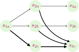
(a) Combination lock $(H=2)$.

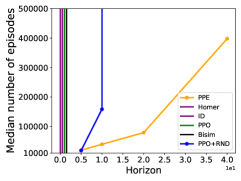
(b) Regret plot

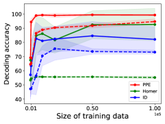
(c) Decoding accuracy

Figure 2: Results on combination lock. Left: We show the latent transition dynamics of combination lock. Observations are not shown for brevity. Center: Shows minimal number of episodes needed to achieve a mean regret of at most $\nicefrac{{V(\pi^{\star})}}{{2}}$. Right: State decoding accuracy (in percent) of decoders learned by different methods. Solid lines implies no exogenous dimension while dashed lines imply an exogenous dimension of 100.

We evaluate ${\tt PPE}$ on two domains: a challenging exploration problem called combination lock to test whether ${\tt PPE}$ can learn an optimal policy and an accurate state decoder, and a visual-grid world with complex visual representations to test whether ${\tt PPE}$ is able to recover the latent dynamics.

Combination Lock Experiments.

The combination lock problem is defined for a given horizon $H$ by an endogenous state space $\mathcal{S}=\{s_{1,a}\}\cup\{s_{h,a},s_{h,b},s_{h,c}\}_{h=2}^{H}$, an exogenous state space $\Xi=\{0,1\}^{H}$, an action space $\mathcal{A}$ with 10 actions, and a deterministic endogenous start state of $s_{1,a}$. For any state $s_{h,g}$ we call $g$ as its type which can be $a,b$ or $c$. States with type $a$ and $b$ are considered good states and those with type $c$ are considered bad states. Each instance of this problem is defined by two good action sequences $(a_{h})_{h=2}^{H},(a^{\prime}_{h})_{h=2}^{H}$ with $a_{h}\neq a^{\prime}_{h}$, which are chosen uniformly randomly and kept fixed throughout training. At $h=1$, the agent is in $s_{1,a}$ and action $a_{1}$ leads to $s_{2,a}$, $a^{\prime}_{h}$ leads to $s_{2,b}$, and all other actions lead to $s_{2,c}$. For $h>2$, taking action $a_{h}$ in $s_{h,a}$ leads to $s_{h+1,a}$ and taking action $a^{\prime}_{h}$ in $s_{h,b}$ leads to $s_{h+1,b}$. In all other cases involving taking an action in a state $s_{h,g}$, we transition to the next bad state $s_{h+1,c}$. We visualize the latent endogenous dynamics in Figure 2a. The exogenous state evolves as follows: we sample $\xi_{1}$ as a vector in $\{0,1\}^{H}$ by selecting the value of each dimension independently uniformly in $\{0,1\}$. At time step $h$, $\xi_{h}$ is generated from $\xi_{h-1}$ by uniformly flipping each bit in $\xi_{h-1}$ independently with probability 0.1. There is a reward of 1.0 on taking the good action $a_{H,a}$ in $s_{H,a}$ and a reward of 0.1 on taking action $a_{H,b}$ in $s_{H,b}$, and in all other cases the agent gets a reward of 0. This gives a $V(\pi^{\star})=1$, and the probability that a random open loop policy gets this optimal return is $10^{-H}$.

An observation $x$ is generated stochastically from a latent state $z=(s,\xi)$. We map $s$ to a vector $w$ encoding the identity of the state. We concatenate $(w,\xi)$, add Gaussian noise to each dimension, and multiply the result with a Hadamard matrix to generate $x$. See Appendix F for full details. Our construction is inspired by similar combination lock problems in prior work [11, 21] (which did not consider exogenous distractors).

Baseline.

We compare ${\tt PPE}$ with five baselines on the combination lock problem. These include ${\tt PPO}$ [26] which is an actor-critic algorithm, ${\tt PPO+RND}$ [7] which adds an exploration bonus to ${\tt PPO}$ using prediction errors, ${\tt Homer}$ that uses contrastive learning [21], and another algorithm ${\tt ID}$ which is similar to ${\tt Homer}$ but instead of contrastive learning it learns an inverse dynamics model to recover the state abstraction. Lastly, we also compare with ${\tt Bisim}$ that learns a bisimulation metric along with an actor-critic agent ([29]). We use existing publicly available codebases for these baselines. Our implementation of ${\tt PPE}$ very closely follows the pseudo-code in Algorithm 1. We model $\mathcal{F}$ using a two-layer feed-forward network with ReLU non-linearity. We train $\mathcal{F}$ with Adam optimization and use a validation set to do model selection. We refer readers to Appendix F for additional experimental details.

Results.

Figure 2b shows results for values of $H$ in $\{5,10,20,40\}$. For each value of $H$, we plot the minimal number of episodes $n$ needed to achieve a mean regret of at most $\nicefrac{{V(\pi^{\star})}}{{2}}=0.5$. We run each algorithm 5 times with different seeds and report the median performance. If an algorithm is unable to achieve the desired regret in $5\times 10^{5}$ episodes then we set $n=\infty$. We observe that ${\tt PPO}$ is unable to solve the problem at $H=5$. ${\tt PPO+RND}$ is able to solve the problem at $H=5$ and $H=10$, showing the exploration bonus induced by random network distillation helps. However, it is unable to solve the problem for larger values of $H$. We observe that ${\tt Homer}$ and ${\tt ID}$ are also unable to solve the problem for any value of $H$. ${\tt Bisim}$ also fails to solve the problem for any $H\geq 5$. This agrees with the theoretical prediction that ${\tt Bisim}$ provides no learning signal when running in sparse-reward settings. In such settings, there can be many episodes before any reward is received. In the absence of any reward, the bisimulation objective incentivizes mapping all observations to the same representation which is not helpful for further exploration. Lastly, ${\tt PPE}$ is able to solve the problem for all values of $H$ and is significantly more sample efficient than baselines. Since the reward function of the combination-lock problem depends only on the endogenous state, we run ${\tt PPE}$ and then a value-iteration like algorithm (see Appendix D.2) to learn a near optimal policy.

In order to understand the failure of ${\tt Homer}$ and ${\tt ID}$, we investigate the accuracy of the state abstraction learned by these methods and compare that with ${\tt PPE}$. We focus on the combination lock setting with $H=2$ and evaluate the learned decoder for the last time step. As the state abstraction models are invariant to label permutation we use the following evaluation metric: given a learned abstraction for the endogenous state $\hat{\phi}:\mathcal{X}\rightarrow[N]$ we compute $\nicefrac{{1}}{{m}}\sum_{i=1}^{m}{\bf 1}\{\hat{\phi}(x_{i,1})=\hat{\phi}(x_{i,2})\Leftrightarrow\phi^{\star}(x_{i,1})=\phi^{\star}(x_{i,2})\}$, where $\{x_{i,1},x_{i,2}\}_{i=1}^{m}$ are drawn independently from a fixed distribution $D$ with good support over all states. We report the percentage accuracy in Figure 2c. When there is no exogenous noise, ${\tt Homer}$ is able to learn a good state decoder with enough samples while ${\tt ID}$ fails to learn, in accordance with the theory. On inspection, we found that ${\tt ID}$ suffers from the under-abstraction issue highlighted earlier as it has difficulty separating observations from $s_{3a}$ and $s_{3b}$. On adding exogenous noise, the accuracy of ${\tt Homer}$ plummets significantly. The accuracy of ${\tt ID}$ also drops but this drop is mild since unlike ${\tt Homer}$, the ${\tt ID}$ objective is able to filter exogenous noise. Lastly, we observe that ${\tt PPE}$ is always able to learn a good decoder and is more sample efficient than baselines.

Visual Grid World Experiments.

We test the ability of ${\tt PPE}$ to recover the latent endogenous transition dynamics in visual grid-world problem. The agent navigates in a $N\times N$ grid world where each grid can contain a stationary object, the goal, or the agent. The agent’s endogenous state is given by its position in the grid and its direction amongst four possible canonical directions. The agent can take five different actions for navigation. The world is visible to the agent as a $8N\times 8N$ sized RGB image. We add exogenous noise as follows: at the beginning of each episode, we independently sample position, size and color of 5 ellipses. The position and size of these ellipses is perturbed after each time step independent of the action. We project these ellipses on top of the world’s image. Figure 3 shows sampled observations from the $7\times 7$ gridworld that we experiment on. The exogenous state is given by the position, size and color of ellipses and is much larger than $|\mathcal{S}|\leq 4N^{2}$. We model $\mathcal{F}$ using a two-layer convolutional neural network and train it using Adam optimization. We defer the full details of setup to Appendix F.

Since the problem has deterministic dynamics, we can evaluate the accuracy of the learned transition model by measuring it in terms of accuracy of the elimination step (Algorithm 1, line 8), since this step induces our algorithm’s mapping from observations to endogenous latent states. For a fixed $h\in\{2,\cdots,H\}$, let $\nu_{i}$ and $\nu_{j}$ be two paths in $\Psi_{h-1}\circ\mathcal{A}$. We compute two type of errors. Type 1 error computes whether ${\tt PPE}$ merged these paths, i.e., predicted them as mapping to the same abstract state, when they go to different endogenous states. Type 2 error computes whether ${\tt PPE}$ predicted the paths as mapping to different abstract states, when they map to the same endogenous state. We report the total number of errors of both types by summing over all values of $h$ and all pairs of different paths in $\Psi_{h-1}\circ\mathcal{A}$. Type 1 errors are more harmful, since they can lead to exploration failure. Specifically, merging paths going to different states may result in the algorithm avoiding one of the two states when exploring at the next time step. Type 2 errors are less serious but lead to inefficiency due to using redundant paths for exploration. When both errors are 0, then the model recovers the exact latent model up to relabeling.

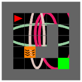
(a) Grid World $h=1$.

(b) Grid World $h=2$.

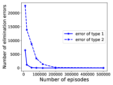
(c) Model Errors

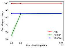
(d) State decoding accuracy

Figure 3: Results on visual grid world. Left two: Shows sampled observations for the first two steps from the visual gridworld domain. The agent is depicted as a red-triangle, lava in orange, walls in grey, and the goal in green. Center Right: Shows errors of type 1 and type 2 made by the ${\tt PPE}$ in recovering the latent endogenous dynamics. Right: State decoding accuracy of ${\tt PPE}$, ${\tt Homer}$ and a random uniform decoder. (see Section 6)

Results.

We report results on learning the model in in Figure 3c. We see that ${\tt PPE}$ is able to reduce the number of type 1 errors down to 0 using $2\times 10^{5}$ episodes per time step. This is important since even a single type 1 error can cause exploration failures. Similarly, ${\tt PPE}$ is able to reduce type 2 errors and is able to get them down to 56 with $5\times 10^{5}$ episodes. This is acceptable since type 2 errors do not cause exploration failures but only cause redundancy. Therefore, at $2\times 10^{5}$ samples, the algorithm makes 0 type 1 errors and just a handful type 2 errors. This is remarkable considering that ${\tt PPE}$ compares roughly $2\times 10^{5}$ pairs of paths in the entire run. Hence, it makes only $\leq 0.03\%$ type 2 errors. Further, the agent is able to plan using the learned transition model and receive the optimal return. We also evaluate the accuracy of state decoding on this problem. We compare the state decoding accuracy of ${\tt PPE}$ and ${\tt Homer}$ at $H=2$ using an identical evaluation setup to the one we used for combination lock. Figure 3d shows the results. As expected, ${\tt PPE}$ rapidly learns a highly accurate decoder while ${\tt Homer}$ performs only as well as a random uniform decoder.

7 Conclusion

In this work, we introduce the EX-BMDP setting, an RL setting that models exogenous noise, ubiquitous in many real-world systems. We show that many existing RL algorithms fail in the presence of exogenous noise. We present ${\tt PPE}$ that learns a multi-step inverse dynamics to filter exogenous noise and successfully explores. We derive theoretical guarantees for ${\tt PPE}$ in near-deterministic setting and provide encouraging experimental evidence in support of our arguments. To our knowledge, this is the first such algorithm with guarantees for settings with exogenous noise. Our work also raises interesting future questions such as how to address the general setting with stochastic transitions, or handle more complex endogenous state representations. Another interesting line of future work direction is the analysis of other approaches that learn multi-step inverse dynamics  [15, 23] and understanding whether these approaches can also provably solve EX-BMDPs.

Acknowlegments

We would like to thank the reviewers for their suggestions and comments. We acknowledge the help of Microsoft’s GCR team for helping with the compute. YE is partially supported by the Viterbi scholarship, Technion.

Appendix

We present the main notations in Table 1 on page 1. The rest of the Appendix is organized as follows:

1. In Appendix A we establish failure cases of several popular approaches for learning an optimal policy in the EX-BMDP model.

2. In Appendix B we study structural properties of an EX-BMDP which highlight some of its key features.

3. In Appendix C we prove Theorem 1 our main performance guarantee on ${\tt PPE}$. There, we show that ${\tt PPE}$ returns an approximate policy cover with cardinality that is bounded by the size of the endogenous state space. Furthermore, the sample complexity of ${\tt PPE}$ does not depend on the cardinality of the exogenous state space at all.

4. In Appendix D we analyze two planning approaches that utilize the output of ${\tt PPE}$ to find a near optimal policy when there exists an access to a reward function. We consider both the cases that the reward function is general, and a reward function that depends on the endogenous state.

5. In Appendix E we supply with several existing results that are used throughout the analysis.

6. In Appendix F we describe in further detalis the experimental setting and supply with additional experiments.

Notation	Meaning
$\mathcal{X}$	Countable observation space. Potentially infinite
$\mathcal{S}$	Finite endogenous state space. Assumed to be finite
$\Xi$	Countable exogenous state space. Potentially infinite
$\mathcal{Z}$	State space given by $\mathcal{Z}=\mathcal{S}\times\Xi$. Potentially infinite.
$\mathcal{A}$	Finite action space
$q$	Emission function ${\mathcal{S}}\rightarrow\Delta(\mathcal{X})$
$T$	Transition function $\mathcal{X}\times\mathcal{A}\rightarrow\Delta(\mathcal{X})$
$H$	Horizon
$\phi^{\star}_{z}$	Maps observation to latent state $\mathcal{X}\rightarrow\mathcal{Z}$
$\phi^{\star}$	Maps observation to endogenous state $\mathcal{X}\rightarrow\mathcal{S}$
$\phi^{\star}_{\xi}$	Maps observation to exogenous state $\mathcal{X}\rightarrow\Xi$
$\mu$	start state distribution (overload $\mu(x)=q(x\mid\phi^{\star}_{z}(x))\mu(\phi^{\star}_{z}(x))$).
$\Pi$	Finite policy class
$\mathcal{F}$	Finite function class $\mathcal{X}\times[N]\rightarrow\mathbb{R}$
$h$	Indicates a time step $h\in[H]$
$\mathcal{M}_{D}$	An $\eta$ close deterministic MDP of the endogenous dynamics
$T_{D}$	Transition function of the $\eta$ close deterministic MDP of the endogenous dynamics
$T_{\xi}$	Transition function of the exogenous state space
$\Psi_{h}$	A policy cover of $h$ step policies
$\pi(1:h)$	The first $h$ step policies of a non-stationary policy of length greater than $h$
$\pi_{h}$	The policy at the $h^{th}$ time step of a non-stationary policy
$\Psi_{h}\circ\mathcal{A}$	Extended policy cover of $\Psi_{h}$, $\Psi_{h}\circ\mathcal{A}=\left\{\pi\textit{ an $h+1$ step policy }:\pi(1:h)\in\Psi_{h},\pi_{h}\in\mathcal{A}\right\}$

Table 1: Notations used in the paper. We start indexing from 1. An episode is given by $(s_{1},a_{1},s_{2},a_{2},\cdots,s_{H},a_{H},s_{H+1})$

Appendix A Failure of Existing Approaches in the Presence of Exogenous Noise

A.1 Failure of Constrastive Learning

In this section we formally show that the objective defined in [21] separates states according to the exogenous part. That is, states that share the same endogenous state, but have different exogenous state will be separated by the Backward Kinematic Inseparability criterion (BKI) on which the objective of HOMER relies upon (see [21], Definition 3). Thus, the abstraction learned by HOMER will have the cardinality of $|{\mathcal{S}}|\times|\Xi|$ and will scale with the number of exogenous states.

Recall the definition of BKI given in [21].

Definition 3 (Backward Kinematic Inseparability).

Two states $(s^{\prime}_{1},\xi^{\prime}_{1}),(s^{\prime}_{2},\xi^{\prime}_{2})\in\mathcal{Z}$ are backward kinematically inseparable if for all distributions $u\in\Delta(\mathcal{Z}\times\mathcal{A})$ supported on $\mathcal{Z}\times\mathcal{A}$ and for all $z=(s,\xi)\in\mathcal{Z},a\in\mathcal{A}$ we have

$$\frac{T(s^{\prime}_{1},\xi^{\prime}_{1}|s,\xi,a)u(s,\xi,a)}{\sum_{\tilde{s},\tilde{\xi},\tilde{a}}T(s^{\prime}_{1},\xi^{\prime}_{1}|\bar{s},\bar{\xi},\bar{a})u(\bar{s},\bar{\xi},\bar{a})}=\frac{T(s^{\prime}_{2},\xi^{\prime}_{2}|s,\xi,a)u(s,\xi,a)}{\sum_{\tilde{s},\tilde{\xi},\tilde{a}}T(s^{\prime}_{1},\xi^{\prime}_{1}|\bar{s},\bar{\xi},\bar{a})u(\bar{s},\bar{\xi},\bar{a})}.$$

The BKI criterion unifies states if they cannot be differentiated w.r.t. any sampling distribution $u$ over the previous time step.

Claim 1.

BKI can splits states with similar endogenous states

This claim is quite generic as we show below - for a very generic class of MDPs BKI splits states with similar endogenous state. Specifically, this occurs when the exogenous process is deterministic.

Proof.

Consider any endogenous dynamics and a deterministic exogenous dynamics, i.e., $T(\xi^{\prime}|\xi)=\operatorname*{1{\hskip-2.5pt}\hbox{I}}\left\{\xi^{\prime}=\xi\right\}$. Let $z^{\prime}_{1}=(s^{\prime},\xi_{1}^{\prime})$ and $z_{2}^{\prime}=(s^{\prime},\xi^{\prime}_{2})$ be two states with similar endogenous dynamics and different exogenous dynamics. Then, BKI splits $z^{\prime}_{1}$ and $z^{\prime}_{2}$, i.e., it treats them as separate states.

Indeed, in this case, by the EX-BMDP model assumptions, it holds that

$$\frac{T(s^{\prime},\xi^{\prime}_{1}|s,\xi,a)u(s,\xi,a)}{\sum_{\tilde{s},\tilde{\xi},\tilde{a}}T(s^{\prime},\xi^{\prime}_{1}|\bar{s},\bar{\xi},\bar{a})u(\bar{s},\bar{\xi},\bar{a})}=\frac{T(s^{\prime}_{1}|s,a)\operatorname*{1{\hskip-2.5pt}\hbox{I}}\left\{\xi^{\prime}_{1}=\xi\right\}u(s,\xi,a)}{\sum_{\tilde{s},\tilde{\xi},\tilde{a}}T(s^{\prime}|\bar{s},\bar{a})\operatorname*{1{\hskip-2.5pt}\hbox{I}}\left\{\xi^{\prime}_{1}=\xi\right\}u(\bar{s},\bar{\xi},\bar{a})}$$

$$\neq\frac{T(s^{\prime},\xi^{\prime}_{2}|s,\xi,a)u(s,\xi,a)}{\sum_{\tilde{s},\tilde{\xi},\tilde{a}}T(s^{\prime},\xi^{\prime}_{2}|\bar{s},\bar{\xi},\bar{a})u(\bar{s},\bar{\xi},\bar{a})}=\frac{T(s^{\prime}|s,a)\operatorname*{1{\hskip-2.5pt}\hbox{I}}\left\{\xi^{\prime}_{2}=\xi\right\}u(s,\xi,a)}{\sum_{\tilde{s},\tilde{\xi},\tilde{a}}T(s^{\prime}|\bar{s},\bar{a})\operatorname*{1{\hskip-2.5pt}\hbox{I}}\left\{\xi_{2}^{\prime}=\xi\right\}u(\bar{s},\bar{\xi},\bar{a})}$$

where the inequality holds since $\xi^{\prime}_{1}\neq\xi^{\prime}_{2}$ (o.w. $z_{1}^{\prime}=z_{2}^{\prime}$). ∎

A.2 Failure of Bisimulation Metric

Recall the definition of the bisimulation relations [14] (also given in [29], Definition 1).

Definition 4 (Bisimulation Relations).

Given an MDP $\mathcal{M},$ an equivalence relation $B$ between states is a bisimulation relation if for all states $s_{i},s_{j}\in{\mathcal{S}}$ that are equivalent under $B$ it holds that

1. $r(s_{i},a)=r(s_{j},a)\quad\forall a\in\mathcal{A}$,

2. $\mathbb{P}(G|s_{i},a)=\mathbb{P}(G|s_{j},a)\quad\forall a\in\mathcal{A},G\in{\mathcal{S}}_{B}$

where ${\mathcal{S}}_{B}$ is the partition of ${\mathcal{S}}$ under the relation $B$ and $\mathbb{P}(G|s,a)=\sum_{s^{\prime}}T(s^{\prime}|s,a)$.

Let $d$ be some distribution over ${\mathcal{S}}$. We say that an equivalence relation $B$ is a $d$-restricted bisimulation relation if Definition 4 holds for all $s\in{\mathcal{S}}$ such that $d(s)>0$. That is, if $B$ is a bisimulation for all states in the support of $d$. Indeed, we have no information on states that are not in the support of $d$. For this reason, we cannot obtain any information on these states.

Claim 2 (With no reward function bismulation may unify all states).

Assume that $r(s,a)=0$ for all states $s\in{\mathcal{S}}$ for which $d(s)>0$, i.e., in the support of $d$. Then, the abstraction $\phi(s)=1$ (i.e., merge all states into a single state) for all $s\in{\mathcal{S}}$ is a valid $d$-restricted bisumlation relation.

Proof.

We show this abstraction is a valid $d$-restricted relation.

1. For all states restricted to $d$, meaning $s\in\left\{s\in{\mathcal{S}}:d(s)>0\right\}$ it holds that $r(s,a)=0$ for all $a\in\mathcal{A}$. Thus, the first requirement of Definition 4 is satisfied.

2. When all states are merges it holds that $G=\Omega$. Thus, $\mathbb{P}(G|s_{i},a)=\mathbb{P}(G|s_{j},a)=1$, and the second requirement of Definition 4 is satisfied.

∎

A.3 Failure of Inverse Dynamics

We describe a totally deterministic setting where Inverse Dynamics (ID) fails. We comment that the counter-example for ID supplied by [21] has stochastic starting state. In this section, we show that even for a deterministic MDP with deterministic starting state ID fails. Specifically, we assume access to an exact solution $f_{\star}$ of a regression oracle that learns ID. Then, we show that a naive approach that uses $f_{\star}$ (see Algorithm 2) fails to return a policy cover.

Algorithm 2 Exact Inverse Dynamics for Deterministic Initial State

1:$\Psi_{1}=\emptyset$

2:for $h=1,\ldots,H-1$ do

3:     Set the sampling distribution $\mu$ to be ${\tt Unf}(\Psi_{h})$

4:     Get $f_{\star}$ that exactly minimizes the loss

$$\mathbb{E}_{x\sim\mu,a\sim{\tt Unf}(\mathcal{A}),x^{\prime}\sim T(\cdot|x,a)}\left[\left(f(a|x,x^{\prime})-\mathbb{P}_{\mu}(a|x,x^{\prime})\right)^{2}\right]$$

5:     Get a consistent ID abstraction (see Definition 5) $\phi:\mathcal{X}\rightarrow[N]$

6:     Set the policy cover for next time as $\Psi_{h+1}=\left\{\pi_{i}^{\star}\right\}_{i=1}^{N}$ where $\pi_{i}^{\star}$ is a deterministic policy that maximizes the reaching probability to the event $\phi(x)=i$.

We start by formally defining the ID abstraction.

Definition 5 (Inverse Dynamics Consistency).

Two observations $x^{\prime}_{1},x_{2}^{\prime}\in\mathcal{X}$ are consistent under the ID and an initial distribution $\mu$ if $\forall x\in\mathcal{X},a\in\mathcal{A}$ either

1. $\mathbb{P}_{\mu}(a|x,x^{\prime}_{1})=\mathbb{P}_{\mu}(a|x,x^{\prime}_{2})$,

2. or either one of the following holds (i) $\mathbb{P}_{\mu}(x,x^{\prime}_{1})=0$, (ii) $\mathbb{P}_{\mu}(x,x^{\prime}_{2}|{\tt Unf}(\mathcal{A}))=0$.

where $x\sim\mu$ and $x_{1}^{\prime},x_{2}^{\prime}\sim T(\cdot|x,a)$.

Relaying on this notion, we define an ID abstraction as follows.

Definition 6 (Inverse Dynamics Abstraction).

We say that an abstraction $\phi:\mathcal{X}\rightarrow[N]$ is an ID abstraction if for all $x_{1}^{\prime},x_{2}^{\prime}\in\mathcal{X}$ for which $\phi(x_{1}^{\prime})=\phi(x_{2}^{\prime})$ it holds that $x_{1}^{\prime},x_{2}^{\prime}$ are consistent under the ID according to Definition 5.

Before addressing the problem that arises relying on the ID abstraction we elaborate on this definition, and specifically part two of its. We claim that this part is necessary to make the ID abstraction well defined. We motivate this definition by the two following arguments.

First, the ID object is a conditional probability function, $\mathbb{P}_{\mu}(a|x,x^{\prime})$. Thus, for $\mathbb{P}_{\mu}(x,x^{\prime})=0$ the conditional probability is not well defined. Indeed, part two of Definition 5 is a possible solution to this issue – without it, the definition of the ID abstraction is not mathematically defined.

Second, a regression oracle that learns $\mathbb{P}_{\mu}(a|x,x^{\prime})$ is not affected – i.e., has similar loss – for all pairs $(x,x^{\prime})$ for which $\mathbb{P}_{\mu}(x,x^{\prime}|{\tt Unf}(\mathcal{A}))=0$. That is, the loss of any $f_{\star}(a|x,x^{\prime})$ that approximates $P_{\mu}(a|x,x^{\prime})$ is not affected by values of $f_{\star}(a|x,x^{\prime})$ for which $\mathbb{P}_{\mu}(x,x^{\prime}|{\tt Unf}(\mathcal{A}))=0$. Thus, the output of the regression oracle $f_{\star}$ can have arbitrary values on these pairs. This may result in $f_{\star}(a|x,x_{1}^{\prime})=f_{\star}(a|x,x_{2}^{\prime})$ for observations for which $\mathbb{P}_{\mu}(x,x^{\prime}_{1}|{\tt Unf}(\mathcal{A}))=0$ or $\mathbb{P}_{\mu}(x,x^{\prime}_{2}|{\tt Unf}(\mathcal{A}))=0$. Put it differently, when learning $\mathbb{P}_{\mu}(a|x,x^{\prime})$ we cannot get any information outside the support of $\mathbb{P}_{\mu}(x,x^{\prime}|{\tt Unf}(\mathcal{A}))=0$ and, thus, the values for these $(x,x^{\prime})$ pairs can be arbitrary.

We say two observations $x^{\prime}_{1},x_{2}^{\prime}$ have no shared common parent if for any $x$ such that $\mathbb{P}_{\mu}(x,x^{\prime}_{1}|{\tt Unf}(\mathcal{A}))>0$ it $\mathbb{P}_{\mu}(x,x^{\prime}_{2}|{\tt Unf}(\mathcal{A}))=0$ and vice-versa. Our counter example relies on the following observation.

Claim 3 (Inverse Dynamics may Merge Observations with no Shared Parent).

If two observations $x_{1}^{\prime},x_{2}^{\prime}$ have no shared common parent then merging these states is always a consistent ID abstraction according to Definition 5.

This claim is a direct consequence of part two of Definition 5: if for all $x$ it holds that either $\mathbb{P}_{\mu}(x,x^{\prime}_{1}|{\tt Unf}(\mathcal{A}))=0$ or $\mathbb{P}_{\mu}(x,x^{\prime}_{2}|{\tt Unf}(\mathcal{A}))=0$ then the two observations $x_{1}^{\prime},x_{2}^{\prime}$ may always be merged while resulting in a consistent abstraction according to the ID abstraction.

With this observation at hand, we construct a simple deterministic MDP for which an ID abstraction merges states that should not be merged; in the sense that no deterministic policy can reach both states.

Proposition 1 (Failure of Inverse Dynamics).

The exists a deterministic MDP such that Algorithm 2 does not return a policy cover on the states on the second time step.

Proof.

Consider the MDP in Figure 2, (a). At $h=1$, a consistent ID abstraction must separate the states $s_{2a},s_{2b},s_{2c}$ and $s_{2c}$. Thus,Algorithm 2 separates all states at $h=1$. However, at $h=2$, since $s_{3a}$ and $s_{3b}$ share no common parent, a consistent ID abstraction may merge these states (due to Claim 3).

Then, since our policy class contains only deterministic policies, we get that necessarily at the end of the $h=2$ iteration, the policy cover that Algorithm 2 returns does not contain a policy that reaches either $s_{3a}$ or $s_{3b}$. That holds since any deterministic policy that maximizes the reaching probability to $s_{3a}\cup s_{3b}$ will hit either $s_{3a}$ or $s_{3b}$. Thus, one of these states will not be reached by the policy cover. ∎

A.4 Bellman Rank Depends on the Exogenous State Cardinally

Proposition 2 (Bellman Rank Depends on the Exogenous State Cardinality).

There exists an Exogenous Block MDP $\mathcal{M}$, policy class $\Pi$, and value function class $\mathcal{F}$ with the following properties: (1) the endogenous state has size $2$, (2) the exogenous state has size $d$, (3) $|\Pi|=|\mathcal{F}|=O(d)$, (4) the optimal policy and value function are in $\Pi,\mathcal{F}$ respectively, and (5) the $(\mathcal{F},\Pi)$ bellman rank is $\Omega(d)$. Additionally, Olive has sample complexity $\Omega(\textrm{poly}(d)/\epsilon^{2})$ to learn an $\epsilon$-optimal policy.

Proof.

We construct the Exogenous Block MDP as follows. Let the horizon be $H$ and set the starting endogenous state to be labeled $g_{1}$. From $g_{1}$ there are two actions: action $a_{1}$ transits to $g_{2}$ while action $a_{2}$ transits to $b_{2}$. We repeat this $H-1$ times randomizing the good and bad action at each level, to arrive at either $g_{H}$ or $b_{H}$. (Here $g$ denotes “good” and $b$ denotes “bad”.) Let $a_{h}^{\star}$ denote the good action at time $h$ and $\tilde{a}_{h}$ denote the bad action at time $h$.

There are no actions at time $H$ and from $g_{H}$ the agent always receives reward $1$, while from $b_{H}$ the agent always receives reward $0$. There are no intermediate rewards. The exogenous state $\xi$ does not change across time and, at the beginning of the episode, $\xi$ is drawn uniformly from $[d]$.

The policy class $\Pi$ is defined as $\Pi=\{\pi_{\star},\pi_{1},\ldots,\pi_{d}\}$ where $\pi_{\star}((g_{h},\cdot))=a_{h}^{\star}$ and $\pi_{i}$ agrees with $\pi_{\star}$ everywhere, except for at state $(g_{H-1},i)$ where it takes $\tilde{a}_{H-1}$. In other words, $\pi_{i}$ defects from the optimal policy only in the good state at time $H-1$ when the exogenous variable $\xi=i$. Meanwhile, the value function class is $\mathcal{F}=\{f_{\star},f_{1},\ldots,f_{d}\}$ where $f_{\star}$ is the optimal value function which satisfies

$$f_{\star}((g_{h},\cdot))=1,\qquad f_{\star}((b_{h},\cdot))=0$$

and $f_{i}$ deviates from the $f_{\star}$ only on state $(b_{H},i)$, where $f_{i}((b_{H},i))=1$.

First observe that $(f_{i},\pi_{i})$ is clearly bellman consistent at all time steps except for the time step $H$, since $f_{i}$ predicts $1$ at all states up to time $H-1$ and on all states visited by $\pi_{i}$ at time $H$.

Now, let us examine the bellman error on roll-in $\pi_{j}$ for value function/policy pair $(f_{i},\pi_{i})$ at the last time. First, the state distribution visited by $\pi_{j}$ at time $H$ is $\textrm{Unif}(\{g_{H},k\}_{k\neq j}\cup\{b_{H},j\})$. If $i\neq j$ then $(f_{i},\pi_{i})$ has zero bellman error on all of these states since it correctly predicts that the reward is $1$ in the good state and it correctly predicts that the reward is $0$ on the bad state $(b_{H},j)$.

On the other hand, if $i=j$ then the bellman error is $1/d$, since $f_{j}$ incorrectly predicts that the reward is $1$ on the bad state. Thus we see that

$$\mathcal{E}_{H}(\pi_{i},(g_{j},\pi_{j})):=\mathbb{E}_{(s_{H},\xi_{H},r_{H})\sim\pi_{i}}\left[g_{j}(s_{H},\xi_{H})-r_{H}\right]=\frac{{\bf 1}\{i=j\}}{d}.$$

This verifies that the bellman rank is $d$.

Regarding Olive, note that the value functions are all bellman consistent at the first $H-1$ time steps. In particular,

$$\forall h\leq H-1:\mathbb{E}_{\pi_{i}}[f_{i}((g_{h},\xi))-f_{i}((s_{h+1},\xi))]=0$$

Thus Olive is unable to eliminate functions using data at the first $H-1$ time steps. Additionally even with perfect evaluation of expectation, due to adversarial tie breaking, Olive may take $\Omega(d)$ iterations to find the optimal policy, since it may cycle through $\pi_{1},\ldots,\pi_{d}$ eliminating one at a time.

This argument can be extended to get $poly(d)/\epsilon^{2}$ sample complexity using standard technique. To prove a lower bound for the sample complexity of OLIVE we adjust the problem by making the rewards $1/2$ and $1/2+\epsilon$. Then, to eliminate a bad policy, we need to estimate the Bellman errors to accuracy of $\epsilon/d$. This results in an $poly(d)/\epsilon^{2}$ lower bound for the sample complexity of OLIVE.

∎

A.5 Failure of FLAMBE Agarwal et al. [2].

In Agarwal et al. [2] the authors studied a representation learning problem for the linear MDP setting and suggested an algorithm, FLAMBE, that provably explores while learning the representation feature map of the linear MDP model. Their algorithm relies on a model-based approach to factorize the transition dynamics. However, focusing on the dynamics in observation space forces the modeling of the exogenous state as well, and the dimension of the factorization that they learn can scale with $|\Xi|$ (similar to the Bellman rank), leading to a $\text{poly}(|\Xi|)$ sample complexity for their approach.

A.6 Failure of auto-encoding approaches

Much prior work uses auto-encoding or other unsupervised techniques for representation learning in RL. Examples include scalable count-based exploration methods [28] and CURL [20]. However, as these methods do not leverage the temporal nature of reinforcement learning, it is easy to see that the representations discovered may not be useful or relevant for exploration or policy learning, without relying heavily on inductive biases. More concretely, an autoencoding approach that aims to minimize reconstruction error on observations would prefer to memorize high-entropy irrelevant noise over lower-entropy relevant state information (see figure 4c in [21]). Unfortunately, the resulting learned representation may omit state information that is crucial for downstream planning.

Appendix B Structural Results for EX-BMDP

In this section we prove several useful structural results about the EX-BMDP model which will be essential for later analysis. A key definition which will be useful is the notion of endogenous policy. We define the class of endogenous policies $\Pi_{d}$ as the policies that depend only on the endogenous part of the state. Formally, a policy $\pi\in\Pi_{d}$ has the property that for all $x\in\mathcal{X}:\,\,\,\pi(a|x)=\pi(a|\phi^{\star}(x))$. Restated, an endogenous policy chooses the same actions for a fixed endogenous state across varying exogenous states and observations. See that open loop policies (see definition in Section 2), which commit to a sequence of actions prior to the interaction, are always endogenous policies, since this sequence of actions is independent of the exogneous noise.

Proposition 3 (Consequence of Endogenous Policy).

Let $\pi\in\Pi_{d}$. Then, for any $h\in[H]$ it holds that $\mathbb{P}_{h}(z|\pi)=\mathbb{P}_{h}(s|\pi)\mathbb{P}_{h}(\xi).$ Furthermore, there exists $\pi\in\Pi_{NS}\backslash\Pi_{d}$ such that $\mathbb{P}_{h}(z|\pi)\neq\mathbb{P}_{h}(s|\pi)\mathbb{P}_{h}(\xi).$

Proof.

First claim. We prove the result by induction.
Base case $h=1$. The base case follows from the model assumption, that is,

$$\mathbb{P}_{h=1}(z|\pi)=\mu(z)=\mu(s)\mu_{\xi}(\xi).$$

Induction step. Assume the claim holds for $h$. We show it also holds for $h+1$ for $\pi\in\Pi_{d}$. For any $z\in\mathcal{Z}$, or, equivalently $z=(s,\xi)$ for $s\in\mathcal{S},\xi\in\Xi$, it holds that

$$\mathbb{P}_{h+1}(z|\pi)=\sum_{z_{h}\in\mathcal{Z}}\mathbb{P}_{h+1}(z,z_{h-1}|\pi)$$ (Law of total probability)

$$=\sum_{z_{h}\in\mathcal{Z}}\mathbb{P}_{h}(z_{h}|\pi)T(z|z_{h},\pi)$$ (Bayes’ theorem & Markovian dynamics)

$$=\sum_{s\in\mathcal{S},\xi\in\Xi}\mathbb{P}_{h}(s_{h}|\pi)\mathbb{P}_{h}(\xi_{h})T(z|z_{h},\pi)$$ (Induction hypothesis)

$$=\sum_{s\in\mathcal{S},\xi\in\Xi}\mathbb{P}_{h}(s_{h}|\pi)\mathbb{P}_{h}(\xi)T(s|s_{h},\pi)T(\xi|\xi_{h}) \pi\in\Pi_{d}$$ ( and EX-BMDP definition)

$$=\sum_{s\in\mathcal{S}}\mathbb{P}_{h}(s_{h}|\pi)T(s|s_{h},\pi)\sum_{\xi\in\Xi}\mathbb{P}_{h}(\xi)T(\xi|\xi_{h})$$

$$=\mathbb{P}_{h+1}(s|\pi)\mathbb{P}_{h+1}(\xi),$$

which concludes the proof.

Second claim. Consider an MDP with $H=2$. The endogenous state is $b_{d}\in\left\{0,1\right\}$, the exogenous state is $b_{\xi}\in\left\{0,1\right\}$ and the full state is $z=\left\{b_{d},b_{\xi}\right\}$. At the initial time step $b_{d}=1$ and $b_{\xi}\sim{\tt Unf}(\left\{0,1\right\})$. Furthermore, the MDP is stationary, and its dynamics is given as follows. The exogenous state is fixed along trajectory,

$$T(b_{\xi}^{\prime}=1|b_{\xi}^{\prime}=1)=T(b_{\xi}^{\prime}=0|b_{\xi}^{\prime}=0)=1.$$

The action set is of size two, $\mathcal{A}=\left\{0,1\right\}$, the endogenous dynamics evolves as

$$T(b_{d}^{\prime}=1|b_{d}=1,a=0)=T(b_{d}^{\prime}=0|b_{d}=1,a=1)=1$$

that is, applying $a=1$ the endogenous state switches to $0$ and applying $a=0$ leaves the endogenous state at $1$.

Let the policy be

$$\pi(a=1|b_{\xi})=\begin{cases}1&b_{\xi}=1\\ 0&o.w.\end{cases},$$

and observe it depends on the exogenous state.

We show that the next state distribution does not decouple the endogenous and exogenous part of the state space.

$$\mathbb{P}_{h=2}(z|\pi)=\mathbb{P}_{h=2}(b_{\xi})\mathbb{P}_{h=2}(s|\pi,\xi)$$

$$=0.5\left(\operatorname*{1{\hskip-2.5pt}\hbox{I}}\left\{b_{\xi}=1,s=0\right\}+\operatorname*{1{\hskip-2.5pt}\hbox{I}}\left\{b_{\xi}=0,s=1\right\}\right)$$

$$\neq\mathbb{P}_{h=2}(s|\pi)\mathbb{P}_{h=2}(b_{\xi})=0.25.$$

∎

Proposition 4 (Existence of Endogenous Policy Cover).

Given an EX-BMDP, for any $h\in[H]$, let $\Psi_{h}$ be an endogenous policy cover of the endogenous dynamics, that is $\Psi_{h}\subseteq\Pi_{d}$ and for all $s\in\mathcal{S}$, $\max_{\pi\in\Psi_{h}}\mathbb{P}_{h}(s|\pi)=\max_{\pi}\mathbb{P}_{h}(s|\pi)$. Then, $\Psi_{h}$ is also a policy cover for the full EX-BMDP, that is: $\max_{\pi\in\Psi_{h}}\mathbb{P}_{h}(z|\pi)=\max_{\pi}\mathbb{P}_{h}(z|\pi)$.

Proof.

Let $\Pi_{NS}$ be the set of tabular policies, $\pi\in\Pi_{NS}$ is a mapping $\pi:\mathcal{Z}\rightarrow\mathcal{A}$. Fix $\bar{z}\in\mathcal{Z}_{h}$, where $\bar{z}=\left(\bar{s},\bar{\xi}\right)$ for some $\bar{s}$ and $\bar{\xi}$ by the EX-BMDP model assumption and fix $h\in[H]$. We not show that for $\bar{z}$ there exists an optimal policy which is also endogenous policy that reaches $\bar{z}$. That is, we show that

$$\max_{\pi\in\Pi_{NS}}\mathbb{P}_{h}(\bar{z}|\pi)=\max_{\pi\in\Pi_{d}}\mathbb{P}_{h}(\bar{z}|\pi).$$

See that

$$\max_{\pi\in\Pi_{NS}}\mathbb{P}_{h}(\bar{z}|\pi)=\max_{\pi\in\Pi_{NS}}\mathbb{E}\left[\sum_{h^{\prime}=1}^{h}r_{h^{\prime}}(z_{h^{\prime}})\mid\pi\right],$$

where $r_{h}(z)=\operatorname*{1{\hskip-2.5pt}\hbox{I}}\left\{z=\bar{z}\right\}$ and zero for all other time steps. We now show inductively that the optimal $Q$ function of the MDP $\mathcal{M}_{\bar{z}}=(\mathcal{Z},\mathcal{A},r,T,h)$ is given by

$$Q^{\star}_{h^{\prime}}(z,a)=\mathbb{P}(\bar{\xi}_{h}|\xi_{h^{\prime}})Q^{\star}_{d,h^{\prime}}(s,a),$$

where $Q^{\star}_{d,h^{\prime}}(s,a)$ does not depend on $\xi$ where $\mathbb{P}(\bar{\xi}_{h}|\xi_{h^{\prime}})$ is the probability the exogenous state at time step $h$ is $\xi_{h}$ given it is $\xi_{h^{\prime}}$ at time step $h^{\prime}$. Specifically, $Q^{\star}_{d,h^{\prime}}(s,a)$ is the optimal $Q$ function on the endogenous MDP $\mathcal{M}_{\bar{s}}=(\mathcal{S},\mathcal{A},r_{d},T,h)$ with reward $r_{d,h}(s)=\operatorname*{1{\hskip-2.5pt}\hbox{I}}\left\{s=\bar{s}\right\}$ and zero for all other time steps, defined on the endogenous state space. This implies that the there exists an optimal policy of $\mathcal{M}_{\bar{z}}$ which is an endogenous policy. The policy

$$\pi^{\star}_{\bar{z}}\in\arg\max_{a}Q^{\star}_{d,h^{\prime}}(s,a)$$

is an endogenous policy which is also optimal.

Base case $h^{\prime}=h$. For the last time step, the claim trivially holds

$$Q^{\star}_{h}(z,a)=\operatorname*{1{\hskip-2.5pt}\hbox{I}}\left\{z=\bar{z}\right\}=\operatorname*{1{\hskip-2.5pt}\hbox{I}}\left\{\xi=\bar{\xi}\right\}\operatorname*{1{\hskip-2.5pt}\hbox{I}}\left\{s=\bar{s}\right\}$$

$$=\mathbb{P}(\bar{\xi}_{h}|\xi_{h})\operatorname*{1{\hskip-2.5pt}\hbox{I}}\left\{s=\bar{s}\right\}=\mathbb{P}(\bar{\xi}_{h}|\xi_{h})Q_{d,h}^{\star}(s,a).$$

Induction step. Assume the claim holds for $h^{\prime}+1$ and prove it holds for $h^{\prime}<h$. The optimal $Q$ function satisfies the following relations for any $h^{\prime}\in[h]$ and $z_{h^{\prime}}\in\mathcal{Z}$, since $r_{h^{\prime}}=0$ for any $h^{\prime}<h$.

$$Q^{\star}_{h^{\prime}}(z_{h^{\prime}},a)=\mathbb{E}\left[\max_{a^{\prime}}Q^{\star}_{h^{\prime}+1}(z_{h^{\prime}+1},a^{\prime})|z_{h^{\prime}},a\right]$$

$$=\mathbb{E}\left[\max_{a^{\prime}}\mathbb{P}(\bar{\xi}_{h}|\xi_{h^{\prime}+1})Q^{\star}_{d,h^{\prime}+1}(s_{h^{\prime}+1},a^{\prime})|z,a\right]$$ (Induction step)

$$=\mathbb{E}\left[\mathbb{P}(\bar{\xi}_{h}|\xi_{h^{\prime}+1})\max_{a^{\prime}}Q^{\star}_{d,h^{\prime}+1}(s_{h^{\prime}+1},a^{\prime})|s_{h^{\prime}},\xi_{h^{\prime}},a\right]$$

$$=\sum_{\xi_{h^{\prime}+1}}\mathbb{P}(\bar{\xi}_{h}|\xi_{h^{\prime}+1})T(\xi_{h^{\prime}+1}|\xi_{h^{\prime}})\sum_{s_{h^{\prime}+1}}T(s_{h^{\prime}+1}|s_{h^{\prime}},a)\max_{a^{\prime}}Q^{\star}_{d,h^{\prime}+1}(s_{h^{\prime}+1},a^{\prime})$$ (Transition assumption)

$$=\mathbb{P}(\bar{\xi_{h}}|\xi_{h^{\prime}})Q^{\star}_{d,h^{\prime}}(s_{h^{\prime}},a),$$

where

$$Q^{\star}_{d,h^{\prime}}(s_{h^{\prime}},a)=\sum_{s_{h^{\prime}+1}}T(s_{h^{\prime}+1}|s_{h^{\prime}},a)\max_{a^{\prime}}Q^{\star}_{d,h^{\prime}+1}(s_{h^{\prime}+1},a^{\prime}),$$

does not depend on the exogenous part of the state space by the induction hypothesis since $Q^{\star}_{d,h^{\prime}+1}(s_{h^{\prime}+1},a^{\prime})$ does not depend on the exogenous part of the state space. Furthermore, $Q^{\star}_{d,h^{\prime}}(s_{h^{\prime}},a)$ satisfy the Bellman equations of $\mathcal{M}_{\bar{s}}$, and, thus, it is the optimal $Q$ function of $\mathcal{M}_{\bar{s}}$.

This concludes the proof of the induction step.

∎

Proposition 5.

Consider an EX-BMDP and assume its reward function depends only on the endogenous part of the state, i.e., for all $x\in\mathcal{X},a\in\mathcal{A}$ and $h\in[H]$, $r_{h}(x,a)=r_{h}(\phi^{\star}(x),a)$. Then, the class of endogenous policies $\Pi_{d}$ contains an optimal policy.

Proof.

Let $r_{h}(x,a)=r_{h}(\phi^{\star}(x),a)$ be a reward function that depends on the endogenous state. To establish the claim, it is sufficient to prove that for any $h\in[H],x\in\mathcal{X},a\in\mathcal{A}$ it holds that $Q^{\star}_{h}(x,a)=Q^{\star}_{h}(\phi^{\star}(x),a)$, where $\left\{Q^{\star}_{h}\right\}_{h=1}^{H}$ is the optimal $Q$ function. This implies that

$$\pi_{h}^{\star}\in\arg\max_{a}Q^{\star}_{h}(\phi^{\star}(x),a),$$

is an optimal policy. Furthermore, $\pi_{h}^{\star}$ is an endogenous policy, since it does not depend on the exogenous part of the state space.

We prove this claim by induction.
Base case, $h=H$. Holds trivially since the reward function depends only on the endogenous state for all $x,a$. Thus, for all $x\in\mathcal{X},a\in\mathcal{A}$

$$Q^{\star}_{H}(x,a)=r_{H}(x,a)=r_{H}(\phi^{\star}(x),a),$$

by assumption.

Induction step, $h$. Assume the claim holds for any $h+1$ for $h<H$. We now show it holds for the $h^{th}$ time step. The optimal $Q$ function satisfies the following relations for all $x\in\mathcal{X},a\in\mathcal{A}$

$$Q^{\star}_{h}(x,a)=r_{h}(x,a)+\mathbb{E}\left[\max_{a}Q^{\star}_{h+1}(x^{\prime},a)|x,a\right]$$

$$=r_{h}(\phi^{\star}(x),a)+\mathbb{E}\left[\max_{a}Q^{\star}_{h+1}(\phi^{\star}(x^{\prime}),a)|x,a\right]$$ (Induction hypothesis & reward assumption)

$$=r_{h}(\phi^{\star}(x),a)+\sum_{s^{\prime},\xi^{\prime}}T(s^{\prime}|\phi^{\star}(x),a)T_{\xi}(\xi^{\prime}|\phi^{\star}_{\xi}(x))\max_{a}Q^{\star}_{h+1}(s^{\prime},a)$$

$$=r_{h}(\phi^{\star}(x),a)+\sum_{s^{\prime}}T(s^{\prime}|\phi^{\star}(x),a)\max_{a}Q^{\star}_{h+1}(s^{\prime},a). \sum_{\xi^{\prime}}T(\xi^{\prime}|\phi^{\star}_{\xi}(x))=1$$ ()

Thus, for all $x\in\mathcal{X},a\in\mathcal{A}$ it holds that $Q^{\star}_{h}(x,a)=Q^{\star}_{h}(\phi^{\star}(x),a)$, i.e., is a function of the endogenous state. ∎

Appendix C Sample Complexity of ${\tt PPE}$

In this section, we present a proof showing that ${\tt PPE}$ learns a policy cover for nearly deterministic EX-BMDPs. More formally, to EX-BMDPS such that the endogenous dynamics is $\eta$ close to a deterministic MDP (see Assumption 1 to quantification of $\eta$ close model).

C.1 Inverse Dynamics Filters Exogenous State

We start by establishing the following result which sheds further intuition on the performance of ${\tt PPE}$. In words, it says that the inverse dynamics objective filters exogenous noise and depends only on the endogenous part of the state.

Lemma 1 (Inverse Dynamics Filters Exogenous State).

For any endogenous policy $\pi\in\Pi_{d}$ and for all $a\in\mathcal{A},h\in[H]$ it holds that $\mathbb{P}_{h}(a,\phi^{\star}(x_{h-1})|x_{h},\pi)=\mathbb{P}_{h}(a,\phi^{\star}(x_{h-1})|\phi^{\star}(x_{h}),\pi)$. If $\pi\in\Pi_{NS}\backslash\Pi_{d}$, $\mathbb{P}_{h}(a,\phi^{\star}(x_{h-1})|x^{(2)}_{h},\pi)\neq\mathbb{P}_{h}(a,\phi^{\star}(x_{h-1})|x^{(2)}_{h},\pi)$ for $\phi^{\star}(x^{(1)}_{h})=\phi^{\star}(x^{(2)}_{h})$.

Proof.

First statement. Proven in Lemma 2 by explicitly applying Bayes’ theorem and the decoupling property of the future state distribution of $\pi\in\Pi_{d}$ (see Proposition 3).

Second statement. Consider an MDP with $H=2$. The endogenous state is $b_{d}\in\left\{0,1\right\}$, the exogenous state is $b_{\xi}\in\left\{0,1\right\}$ and the full state is $z=\left\{b_{d},b_{\xi}\right\}$. At the initial time step $b_{d}=1$ and $b_{\xi}\sim{\tt Unf}(\left\{0,1\right\})$. Furthermore, the MDP is stationary, and its dynamics is given as follows. The exogenous state is fixed along a trajectory,

$$T_{\xi}(b_{\xi}^{\prime}=1|b_{\xi}^{\prime}=1)=T_{\xi}(b_{\xi}^{\prime}=0|b_{\xi}^{\prime}=0)=1.$$

The action set is of size two, $\mathcal{A}=\left\{0,1\right\}$, the endogenous dynamics evolves as

$$T(b_{d}^{\prime}=1|b_{d}=1,a=1)=1-\alpha,\ T(b_{d}^{\prime}=1|b_{d}=1,a=0)=\alpha.$$

Assume the policy is a function of the exogenous state given as follows

$$\pi(a=1|b_{\xi})=\begin{cases}1&b_{\xi}=1\\ 0&b_{\xi}=0\end{cases}.$$

To conclude the proof, let $b^{\prime}_{d},b_{\xi}^{\prime}$ denote the state at the second time step. We show that (suppressing the deterministic event $b_{d}=1$ at the first time step)

$$\frac{\mathbb{P}(a=1|b_{d}^{\prime}=1,b_{\xi}^{\prime}=1)}{\mathbb{P}(a=1|b_{d}^{\prime}=1,b_{\xi}^{\prime}=0)}\neq 1,$$

thus, $\mathbb{P}(a=1|b_{d}^{\prime}=1,b_{\xi}^{\prime}=1)\neq\mathbb{P}(a=1|b_{d}^{\prime}=1,b_{\xi}^{\prime}=0)$.

To prove this, by Bayes’ theorem,

$$\frac{\mathbb{P}(a=1|b_{d}^{\prime}=1,b_{\xi}^{\prime}=1)}{\mathbb{P}(a=1|b_{d}^{\prime}=1,b_{\xi}^{\prime}=0)}=\frac{\mathbb{P}(b_{d}^{\prime}=1,b_{\xi}^{\prime}=1|a=1)}{\mathbb{P}(b_{d}^{\prime}=1,b_{\xi}^{\prime}=0|a=1)}\frac{\mathbb{P}(b_{d}^{\prime}=1,b_{\xi}^{\prime}=0)}{\mathbb{P}(b_{d}^{\prime}=1,b_{\xi}^{\prime}=1)}.$$ (2)

Observe that $\mathbb{P}(b_{d}^{\prime}=1,b_{\xi}^{\prime}=0|a=1)=\mathbb{P}(b_{d}^{\prime}=1,b_{\xi}^{\prime}=1|a=1)=0.5\cdot\alpha$. Thus,

$$\eqref{eq: counter example 2}=\frac{\mathbb{P}(b_{d}^{\prime}=1,b_{\xi}^{\prime}=0)}{\mathbb{P}(b_{d}^{\prime}=1,b_{\xi}^{\prime}=1)}.$$

See that

$$\mathbb{P}(b_{d}^{\prime}=1,b_{\xi}^{\prime}=0)=\mathbb{P}(b_{d}^{\prime}=1|b_{\xi}^{\prime}=0)\mathbb{P}(b_{\xi}^{\prime}=0)=0.5\alpha$$

$$\mathbb{P}(b_{d}^{\prime}=1,b_{\xi}^{\prime}=1)=\mathbb{P}(b_{d}^{\prime}=1|b_{\xi}^{\prime}=1)\mathbb{P}(b_{\xi}^{\prime}=1)=0.5(1-\alpha).$$

Thus, for $a\notin\left\{0,1,0.5\right\}$ we get that

$$\frac{\mathbb{P}(a=1|b_{d}^{\prime}=1,b_{\xi}^{\prime}=1)}{\mathbb{P}(a=1|b_{d}^{\prime}=1,b_{\xi}^{\prime}=0)}=\frac{\alpha}{1-\alpha}\neq 1.$$

∎

The intuition which underlies the construction of the second statement goes as follows. When a policy acts according to the exogenous state information on the exogenous state at time step $h=2$ may change the knowledge we have on the action taken at the previous time step $h=1$.

Lemma 2 (Bayes Optimal Classifier).

Assume that $\pi\in\Pi_{d}$ is an endogenous policy. Then, for every $x,x^{\prime}\in\mathcal{X}_{h},a\in\mathcal{A}$ we have:

$$\mathbb{P}(a,\phi^{\star}(x)\mid x^{\prime},\pi)=\frac{T(\phi^{\star}(x^{\prime})\mid a,\phi^{\star}(x))\mathbb{P}(a,\phi^{\star}(x)\mid\pi)}{\sum_{s\in\mathcal{S},a\in\mathcal{A}}T(\phi^{\star}(x^{\prime})\mid a,s)\mathbb{P}(a,s\mid\pi)}.$$

Proof.

We prove this result by applying Bayes’ Theorem.

$$\mathbb{P}(a,\phi^{\star}(x)\mid x^{\prime},\pi)=\frac{\mathbb{P}(x^{\prime}\mid a,\phi^{\star}(x),\pi)\mathbb{P}(a,\phi^{\star}(x)\mid\pi)}{\sum_{s\in\mathcal{S},a\in\mathcal{A}}\mathbb{P}(x^{\prime}\mid a,s,\pi)\mathbb{P}(a,s\mid\pi)}$$ (3)

Observe that by the model assumption,

$$\mathbb{P}(x^{\prime}\mid a,\phi^{\star}(x),\pi)=q(x^{\prime}|\phi^{\star}(x^{\prime}),\phi^{\star}_{\xi}(x^{\prime}))\mathbb{P}(\phi^{\star}(x^{\prime}),\phi^{\star}_{\xi}(x^{\prime})\mid a,\phi^{\star}(x),\pi).$$ (4)

We focus on the second term. By the law of total probability and by applying Bayes’ theorem,

$$\mathbb{P}(\phi^{\star}(x^{\prime}),\phi^{\star}_{\xi}(x^{\prime})\mid a,\phi^{\star}(x),\pi)=\sum_{\xi}\mathbb{P}(\phi^{\star}(x^{\prime}),\phi^{\star}_{\xi}(x^{\prime})\mid a,\phi^{\star}(x),\xi,\pi)\mathbb{P}(\xi\mid a,\phi^{\star}(x),\pi)$$

$$\underset{(a)}{=}\sum_{\xi}\mathbb{P}(\phi^{\star}(x^{\prime}),\phi^{\star}_{\xi}(x^{\prime})\mid a,\phi^{\star}(x),\xi,\pi)\mathbb{P}(\xi)$$

$$\underset{(b)}{=}\sum_{\xi}T(\phi^{\star}(x^{\prime})\mid a,\phi^{\star}(x))T_{\xi}(\phi^{\star}_{\xi}(x^{\prime})\mid\xi)\mathbb{P}(\xi)$$

$$=T(\phi^{\star}(x^{\prime})\mid a,\phi^{\star}(x))\sum_{\xi}T_{\xi}(\phi^{\star}_{\xi}(x^{\prime})\mid\xi)\mathbb{P}(\xi)$$

$$=T(\phi^{\star}(x^{\prime})\mid a,\phi^{\star}(x))\mathbb{P}(\phi^{\star}_{\xi}(x^{\prime})).$$ (5)

where $(a)$ holds since the policy $\pi\in\Pi_{d}$ followed by a fixed action $a$ is an endogenous policy and $\mathbb{P}(\xi\mid a,\phi^{\star}(x),\pi)=\mathbb{P}(\xi)$ for an endogenous policy due to Proposition 3. The relation $(b)$ holds due to the Markov property of the latent state and the decoupling of the transition model of an EX-BMDP.

Plugging (4) and (5) into (3) we get

$$\mathbb{P}(a,\phi^{\star}(x)\mid x^{\prime},\pi)=\frac{T(\phi^{\star}(x^{\prime})\mid a,\phi^{\star}(x))\mathbb{P}(a,\phi^{\star}(x)\mid\pi)}{\sum_{s\in\mathcal{S},a\in\mathcal{A}}T(\phi^{\star}(x^{\prime})\mid a,s)\mathbb{P}(a,s\mid\pi)}.$$

∎

C.2 Highlevel Analysis Overview of Theorem 1

Analysis overview, deterministic dynamics.

Prior to addressing the near deterministic case, we consider the fully deterministic case. The analysis of this setting highlights the core ideas that are later utilized in the proof.

The idea which underlies the analysis of ${\tt PPE}$ is to prove, in an inductive manner, that at each time step $h\in 2,3.,..H$ the policy cover at $\Psi_{h-1}$ is a minimal policy cover of the endogenous state space. That is, there is a one-to-one correspondence between endogenous states $s\in\mathcal{S}_{h-1}$ and open-loop policies $\nu\in\Psi_{h-1}$ such that for any $s\in\mathcal{S}_{h-1}$ there exists a unique open-loop policy $\upsilon\in\Psi_{h-1}$ that reaches $s$.

The base case holds since the starting state is deterministic. Assume the claim holds for $h-1$. Then, we need to show it holds for $h$. Since $\Psi_{h-1}$ is a minimal policy cover for the endogenous dynamics by a compositionality property of deterministic environments (see Lemma 6), the set of open-loop policies $\Upsilon_{h}=\Psi_{h-1}\circ\mathcal{A}$ in which every policy in $\Psi_{h-1}$ is extended by all actions, is a policy cover for the $h^{th}$ time step. However, it may contain duplicates; two paths may reach to the same endogenous state.

Due to the above reasoning, by eliminating policies from $\Upsilon_{h}$ we can recover a minimal policy cover for the $h^{th}$ time step and to establish to induction step. Let $\nu\in\Upsilon_{h}$ and $f_{h}^{\star}(\nu,x^{\prime})\equiv\mathbb{P}_{h}(\nu|x^{\prime},{\tt Unf}(\Upsilon_{h}))$ be the inverse dynamics which predicts the probability $\nu$ was taken while observing $x^{\prime}$ and following the policy ${\tt Unf}(\Upsilon_{h})$. Due to the one-to-one correspondence between $\left\{(s,a)\right\}_{a\in\mathcal{A},s\in\mathcal{S}_{h-1}}$ and $\Upsilon_{h}$ we expect this function to depend only on the endogenous state (see Proposition 4). Specifically, it is possible to show the following identity on which the elimination criterion of ${\tt PPE}$ is based upon. Let $\Delta^{\star}(i,j)=\mathbb{E}_{x^{\prime}\sim\mathbb{P}_{h}(\cdot|{\tt Unf}(\Upsilon_{h}))}[\left|f_{h}^{\star}(\upsilon_{i},x^{\prime})-f_{h}^{\star}(\upsilon_{j},x^{\prime})\right|]$. For any $\upsilon_{i},\upsilon_{h}\in\Upsilon_{h}$ it holds that

$$\Delta^{\star}(i,j)=\begin{cases}\frac{2}{|\Upsilon_{h}|}&\textit{$\upsilon_{i}$ and $\upsilon_{j}$ lead to different endogenous state}\\ 0&o.w.\end{cases}$$ (6)

Observe that we can learn $f_{h}^{\star}$ to sufficiently good accuracy with respect to the distribution $x^{\prime}\sim\mathbb{P}_{h}(\cdot|{\tt Unf}(\Upsilon_{h}))$ via standard regression guarantees of the MLE (see Theorem 4). Thus, for any $\upsilon_{i},\upsilon_{j}\in\Upsilon_{h}$ we can estimate $\Delta^{\star}(i,j)$ and deduce whether they lead to the same endogenous state, when $\Delta^{\star}(i,j)$ is small, or not, when $\Delta^{\star}(i,j)$ is large. This step is performed in the elimination step if ${\tt PPE}$, line 8. Thus, we can safely eliminate open-loop policies form $\Upsilon_{h}$ that reach that same endogenous state and be left with a minimal policy cover $\Psi_{h}$ for the next time step.

Analysis overview, near deterministic dynamics.

The analysis of the deterministic setting can be generalized to the near deterministic endogenous dynamics by a delicate modification of the above argument.

For this setting, the simplest way we found to extend the argument for the deterministic case goes as follows. We prove via induction that for any $h\in[H]$ the set of open-loop policies $\Psi_{h}$ is a minimal policy cover of the $\eta$ close deterministic endogenous MDP. Specifically, we use similar arguments as for the deterministic case, while replacing (6) with a proper generalization supplied in Lemma 5. Observe that open loop policies are always endogenous policies ; such a policy does not depend on the state and is picked before interacting with the environment. This fact, allows us to use an inverse dynamics objective which filters the exogenous information.

Tho complete the proof, we show that a minimal policy cover of the $\eta$ close deterministic MDP is an $\eta H$ approximate policy cover (see Definition 2). Furthermore, we also show that with this set of policies we can apply the PSDP [5] algorithm to get a near optimal policy when the reward function is an arbitrary function of observations, that might depend on the exogenous part of the state space.

C.3 Proof of Theorem 1

We start by formally defining a minimal policy cover for deterministic dynamics. This definition can be naturally generalized to general MDPs. Nevertheless, since we only study near deterministic dynamics we will only use the next, more specific definition.

Definition 7 (Minimal Policy Cover for Deterministic Endogenous MDP).

Assume that the endogenous dynamics is deterministic. We say that a policy cover $\Psi_{h}$ is minimal for time step $h\in[H]$ if for every $s\in\mathcal{S}_{h}$ there exists a unique path $\upsilon\in\Psi_{h}$ that reaches it, that is $\mathbb{P}(s|\upsilon)=1$.

In this section we supply the proof of Theorem 1.

We now prove Theorem 1 by establishing a more general result that will also be helpful when considering planning algorithms (see Appendix D). See that Theorem 1 is a direct consequence of the second statement of the next result result.

Theorem 2 (Sample Complexity: Policy Cover with ${\tt PPE}$).

Assume that there exists an $\eta\leq\frac{1}{4SH}$ close deterministic MDP for the endogenous dynamics. Let $\delta\in(0,1)$ and assume ${\tt PPE}$ has access to $O\left(S^{2}A^{2}\log\left(\frac{|\mathcal{F}|SAH}{\delta}\right)\right)$ sample for each iteration $h\in[H]$. Then, with probability greater than $1-\delta$ the following holds.

1. For any $h\in[H]$ the policy cover $\Psi_{h}$ is a minimal policy cover of the $\eta$ close near deterministic MDP of the endogenous dynamics.

2. For any $h\in[H]$ the policy cover $\Psi_{h}$ is $\eta H$ approximate policy cover.

Proof.

First statement. To prove this result we prove the following inductive argument. Denote by $\mathcal{M}_{D}$ the $\eta$ close deterministic MDP, by $T_{D}$ its transition function, and let $\mathcal{S}_{h}^{D}$ be the set of reachable states on $\mathcal{M}_{D}$. Let $G_{h}$ be the good event in which at the end of the $h^{th}$ time step for any $s\in\mathcal{S}_{h}^{D}$ there exists a unique path $\upsilon\in\Psi_{h}$ that reaches $s$ on the $\eta$ close deterministic MDP. More formally, let $\mathbb{P}_{h}(\cdot|\nu,T_{D})$ denote the state distribution of time step $h$ on the $\eta$ close deterministic MDP when the open loop policy $\nu$ is applied. Then, the good event $G_{h}$ is defined as follows.

$$G_{h}=\left\{\textit{at the end of the $h^{th}$ time step: }\forall s\in\mathcal{S}_{h}^{D},\exists\textit{ a unique }\nu\in\Psi_{h}\textit{ s.t. }\mathbb{P}_{h}(s|\nu,T_{D})=1\right\}$$ (7)

Conditioning on $G_{0:H}$ it holds that, for all $h\in[H]$, $\Psi_{h}$ is a minimal policy cover of the $\eta$ close deterministic MDP of the endognous dynamics. Hence, to conclude the proof of the first statement, we can prove that $\mathbb{P}(G_{0:H})\geq 1-\delta.$ To do so, and since $\mathbb{P}(G_{0})=1$, it is sufficient to prove that

$$\mathbb{P}(G_{h+1}|G_{0:h})\geq 1-\frac{\delta}{H}$$ (8)

Then by an inductive argument it can be proved that $\mathbb{P}(G_{0:h})\geq 1-\frac{(h-1)\delta}{H}$. Indeed, the base case holds since $\mathbb{P}(G_{0})=1$, and the induction step holds since

$$\mathbb{P}(G_{1}\cap\cdots\cap G_{h+1})=\mathbb{P}(G_{1}\cap\cdots\cap G_{h})\mathbb{P}(G_{h+1}|G_{1}\cap\cdots\cap G_{h})$$

$$\geq\left(1-\frac{(h-1)\delta}{H}\right)\mathbb{P}(G_{h+1}|G_{1}\cap\cdots\cap G_{h})$$ (inductive assumption)

$$\geq\left(1-\frac{(h-1)\delta}{H}\right)\left(1-\frac{\delta}{H}\right)$$ (Assuming (8))

$$\geq 1-\frac{h\delta}{H}.$$

In Lemma 4 we prove that (8) holds and establish the theorem.

Second statement. The endogenous minimal policy cover of the $\eta$ close deterministic MDP of the endogenous dynamics implies an $\eta H$ approximate policy cover for the true EX-BMDP. We formally prove the claim in Lemma 3. ∎

Lemma 3 (Translating Policy Covers).

Let $\mathcal{M}=(\mathcal{Z},\mathcal{A},T,T_{\xi},H,q)$ be an EX-BMDP with $\eta$ near deterministic endogenous dynamics $T_{D}$. Assume that $\Psi_{h}$ is an endogenous minimal policy cover of the $\eta$ near deterministic endogenous for the $h^{th}$ time step. Assume that $\mathcal{M}$ and $\mathcal{M}_{D}$ are $\eta$ close. Then, $\Psi_{h}$ is an $h\eta$ approximate policy cover for $\mathcal{M}$.

Proof.

By Lemma 8 it holds for any $s\in\mathcal{S}_{h}$ that

$$\mathbb{P}_{h}(s|\pi)\geq\mathbb{P}_{h}(s|\pi,T_{D})-\eta h,\textit{ and }\mathbb{P}_{h}(s|\pi)\leq\mathbb{P}_{h}(s|\pi,T_{D})+\eta h.$$ (9)

If $s\in\mathcal{S}_{h}^{D}$ where $\mathcal{S}_{h}^{D}$ is the set of reachable states at $h$ time step on $T_{D}$, there exists a policy $\pi\in\Psi_{h}$ such that $\mathbb{P}_{h}(s|\pi,T_{D})=1$. Thus, due to (9), for any $s\in\mathcal{S}_{h}^{D}$ there exists a policy $\pi\in\Psi_{h}$ such

$$\mathbb{P}_{h}(s|\pi)\geq\mathbb{P}_{h}(s|\pi,T_{D})-\eta h=1-\eta h\geq\max_{\pi\in\Pi_{d}}\mathbb{P}_{h}(s|\pi)-\eta h.$$ (10)

Due to this result, since $\pi\in\Psi_{h}$ is an endogenous policy and by Proposition 3 it holds that for any $\xi\in\Xi$

$$\mathbb{P}_{h}(z|\pi)=\mathbb{P}_{h}(\xi)\mathbb{P}_{h}(s|\pi) \pi\in\Pi_{d}$$ (Proposition 3 & )

$$\geq\max_{\pi\in\Pi_{d}}\mathbb{P}_{h}(\xi)\mathbb{P}_{h}(s|\pi)-\eta h$$ (By (10))

$$=\max_{\pi\in\Pi_{d}}\mathbb{P}_{h}(z|\pi)-\eta h \pi\in\Pi_{d}$$ (Proposition 3 & )

$$=\max_{\pi\in\Pi_{NS}}\mathbb{P}_{h}(z|\pi)-\eta h.$$ (Proposition 4)

Hence, for any $z=(s,\xi)$ where $s\in\mathcal{S}_{h}^{D}$ it holds that there exists $\pi\in\Psi_{h}$ such that

$$\mathbb{P}_{h}(z|\pi)\geq\max_{\pi\in\Pi_{NS}}\mathbb{P}_{h}(z|\pi)-\eta h.$$

Assume that $s\in\mathcal{S}_{h}/\mathcal{S}_{h}^{D}$, that is, it is reachable in $h$ time steps on the true MDP $\mathcal{M}$ but not on the deterministic MDP $\mathcal{M}_{D}$. That is, for any $\pi$ it holds that $\mathbb{P}_{h}(s|\pi,T_{D})=0$. Thus, again by applying (9), it holds that for any $\pi\in\Pi_{d}$

$$\mathbb{P}_{h}(s|\pi)\leq\mathbb{P}_{h}(s|\pi,T_{D})+\eta h=\eta h.$$

Fix $\xi\in\Xi$. By multiplying both sides by $\mathbb{P}_{h}(\xi)$ we get that for any such $z=(s,\xi)$ it holds that

$$\mathbb{P}_{h}(\xi)\max_{\pi\in\Pi_{d}}\mathbb{P}_{h}(s|\pi)=\max_{\pi\in\Pi_{d}}\mathbb{P}_{h}(\xi)\mathbb{P}_{h}(s|\pi)$$

$$=\max_{\pi\in\Pi_{d}}\mathbb{P}_{h}(z|\pi) \pi\in\Pi_{d}$$ (Proposition 3 & )

$$\leq\eta h.$$

On the other hand, by Proposition 4 it holds that

$$\max_{\pi\in\Pi_{d}}\mathbb{P}_{h}(z|\pi)=\max_{\pi\in\Pi_{NS}}\mathbb{P}_{h}(z|\pi).$$

Hence, for any $z=(s,\xi)$ where $s\in\mathcal{S}_{h}/\mathcal{S}_{h}^{D}$ it holds that $\max_{\pi\in\Pi_{NS}}\mathbb{P}_{h}(z|\pi)\leq\eta H$. Hence, excluding policies that try to reach these state does not violate the definition of an $\eta h$ approximate policy cover (see Definition 2).

∎

Lemma 4.

The ${\tt PPE}$ algorithm at the $h^{th}$ time step satisfies that

$$\mathbb{P}(G_{h}|G_{0:h-1})\geq 1-\frac{\delta}{H}$$

where the good event is defined in the proof of Theorem 2. That is, conditioning on the success of ${\tt PPE}$ at previous time-steps, with probability greater than $1-\frac{\delta}{H}$, ${\tt PPE}$ recovers the transition model of $\mathcal{M}_{D}$ between all reachable states at the $h^{th}$ to the $h+1^{th}$ level.

Proof.

We will prove the following claims conditioning on $G_{0:h-1}$. Combining the two concludes the proof of the lemma.

1. Compositionality of policy cover. The extended policy cover $\Upsilon_{h}$ is a super set of a policy cover of the $h^{th}$ time step of the $\eta$ close deterministic transition model.

2. Elimination succeeds. Consider the $i,j$ iteration of the for loop in line 6 of Algorithm 1. If $\upsilon_{i},\upsilon_{j}\in\Upsilon_{h}=\Psi_{h-1}\times\mathcal{A}$ reaches the same endogenous state $s\in\mathcal{S}_{h}$ on the $\eta$-close deterministic MDP, then ${\tt PPE}$ eliminates $\nu_{j}$ from $\Upsilon_{h}$ with probability greater than ${1-\frac{\delta}{(SA)^{2}H}}$.

Taking a union bound on all pairs we get that the elimination procedure succeeds. Thus, ${\tt PPE}$ outputs a perfect policy cover over $\mathcal{S}_{h}^{D}$ with probability greater than $1-\frac{\delta}{H}$. Thus concluding the proof.

We now prove the two claims.

Claim 1. Conditioning on $G_{0:h-1}$ it holds that $\Psi_{h-1}$ is a perfect policy cover for the $\eta$ close deterministic transition model. By Lemma 6, utilizing the fact that $\Psi_{h-1}$ is a perfect policy cover, it holds that $\Upsilon_{h}=\Psi_{h-1}\times\mathcal{A}$ is a policy cover for the $h^{th}$ time step for the $\eta$ close determinstic dynamics. That is, for any $s\in\mathcal{S}_{h}^{D}$ there exists at least a single path $\upsilon\in\Upsilon_{h}$ that reaches $s$ on the $\eta$ close deterministic MDP.

Claim 2. Let $\upsilon_{i},\upsilon_{j}\in\Upsilon_{h}$ be a fixed and different paths in the extended policy cover at the $h^{th}$ time step, $\Upsilon_{h}$. Let the empirical and the expected disagreement w.r.t. $f\in\mathcal{F}$ be defined as follows.

$$\widehat{\Delta}(i,j;f)=\frac{1}{N}\sum_{i=1}^{N}\left|f(\upsilon_{i}|x_{h,n})-f(\upsilon_{j}|x_{h,n})\right|$$

$$\Delta(i,j;f)=\mathbb{E}_{x_{h}\sim\mathbb{P}(\cdot|\mathcal{U}(\Upsilon_{h}))}\left[\left|f(\upsilon_{i}|x_{h})-f(\upsilon_{j}|x_{h})\right|\right].$$

Observe that $\widehat{\Delta}(i,j;f)$ is an average of $N$ i.i.d. and bounded in $[0,1]$ random variables. Furthermore, the expectation of the random variables is exactly $\Delta(i,j;f)$. Thus, for any fixed $\upsilon_{i},\upsilon_{j}\in\Upsilon_{h}$ and $f\in\mathcal{F}$, given $N=O\left(|\Upsilon_{h}|^{2}\log\left(\frac{1}{\delta}\right)\right)$ samples, due to Hoeffding’s inequality, it holds that

$$\left|\widehat{\Delta}(i,j;f)-\Delta(i,j;f)\right|\leq\frac{1}{24|\Upsilon_{h}|},$$ (11)

with probability greater than $1-\delta$. Applying the union bound on all $f\in\mathcal{F}$ we get that (11) holds with probability greater than $1-\frac{\delta}{|\Upsilon_{h}|^{2}H}$ for all $f\in\mathcal{F}$ given

$$N=O\left(|\Upsilon_{h}|^{2}\log\left(\frac{|\mathcal{F}||\Upsilon_{h}|H}{\delta}\right)\right).$$

Let $\widehat{\Delta}(i,j)\equiv\widehat{\Delta}(i,j;\hat{f}_{h}),\Delta(i,j)\equiv\Delta(i,j;\hat{f}_{h})$ where $\hat{f}_{h}$ is the solution of the maximum liklihood objective. Since (11) holds w.r.t. $f\in\mathcal{F}$, it implies that

$$\left|\widehat{\Delta}(i,j)-\Delta(i,j)\right|\leq\frac{1}{24|\Upsilon_{h}|},$$ (12)

with probability greater than $1-\frac{\delta}{|\Upsilon_{h}|^{2}H}$. Furthermore, notice that

$$\left|\Delta^{\star}(i,j)-\Delta(i,j)\right|$$

$$=\left|\mathbb{E}_{x_{h}\sim\mathbb{P}(\cdot|\mathcal{U}(\Upsilon_{h}))}\left[\left|f_{h}^{\star}(\upsilon_{i}|x_{h})-f_{h}^{\star}(\upsilon_{j}|x_{h})\right|-\left|\hat{f}_{h}(\upsilon_{i}|x_{h})-\hat{f}_{h}(\upsilon_{j}|x_{h})\right|\right]\right|$$

$$\leq\mathbb{E}_{x_{h}\sim\mathbb{P}(\cdot|\mathcal{U}(\Upsilon_{h}))}\left[\left|\hat{f}_{h}(\upsilon_{i}|x_{h})-f_{h}^{\star}(\upsilon_{i}|x_{h})\right|\right]+\mathbb{E}_{x_{h}\sim\mathbb{P}(\cdot|\mathcal{U}(\Upsilon_{h}))}\left[\left|\hat{f}_{h}(\upsilon_{j}|x_{h})-f_{h}^{\star}(\upsilon_{j}|x_{h})\right|\right]$$

$$\leq 2\epsilon,$$ (13)

where the second relation holds since $\left||a|-|b|\right|\leq|a-b|$ due to the triangle inequality, and the third relation holds with probability greater than $1-\frac{\delta}{|\Upsilon_{h}|^{2}H}$ due to Theorem 4 where $2\epsilon=\frac{2}{24|\Upsilon_{h}|}$ for $N=O\left(|\Upsilon_{h}|^{2}\log\left(\frac{|\mathcal{F}||\Upsilon_{h}|^{2}H}{\delta}\right)\right)$. Observe that Theorem 4 is applicable due to the realizability Assumption 2.

By combining (12) and (13) it holds that

$$\left|\widehat{\Delta}(i,j)-\Delta^{\star}(i,j)\right|\leq 2\epsilon+\frac{1}{24|\Upsilon_{h}|}=\frac{1}{8|\Upsilon_{h}|}.$$ (14)

By taking a union bound on all $\nu_{i},\nu_{j}\in\Upsilon_{h}$ we get that (14) for all $\nu_{i},\nu_{j}\in\Upsilon_{h}$ with probability greater than $1-\frac{\delta}{H}.$

Finally, by Lemma 5 it holds that

$$\begin{cases}\left|\Delta^{\star}(i,j)\right|\leq\frac{1}{4|\Upsilon_{h}|}&\textit{$\upsilon_{i}$ and $\upsilon_{j}$ reach the same endogenous state on $\mathcal{M}_{D,\eta}$}\\ \left|\Delta^{\star}(i,j)\right|\geq\frac{1}{|\Upsilon_{h}|}&o.w.\end{cases}$$

if $\Psi_{h-1}$ is a perfect policy cover, which holds conditioning on $G_{h-1}$. This fact, together with (14) implies that with probability greater than $1-\frac{\delta}{H}$

$$\begin{cases}\left|\widehat{\Delta}(i,j)\right|\leq\frac{3}{8|\Upsilon_{h}|}&\textit{$\upsilon_{i}$ and $\upsilon_{j}$ reach the same endogenous state on $\mathcal{M}_{D,\eta}$}\\ \left|\widehat{\Delta}(i,j)\right|\geq\frac{7}{8|\Upsilon_{h}|}&o.w.\end{cases}$$

Thus, for any part $\nu_{i},\nu_{j}$ the elimination process succeeds with probability greater than $1-\frac{\delta}{H}$ since we set the elimination threshold to be $\frac{5}{8|\Upsilon_{h}|}$ in line 8 of Algorithm 1. That is, with probability greater than $1-\frac{\delta}{H}$ at the end of the $h^{th}$ episode we are left with a perfect policy cover on the $\eta$ close deterministic MDP, conditioning on $G_{0:h-1}$. ∎

The following lemma highlights the existence of margin for MDPs which are $\eta$ close to a deterministic MDP for $\eta\leq 1/(4|\mathcal{S}|H).$

Lemma 5 (Existence of Margin for Inverse Path Prediction Near Deterministic Dynamics).

Assume the transition model is $\eta$ close to deterministic dynamics. Let $\Psi_{h-1}$ be a perfect policy cover of the $\eta$ close deterministic dynamics and $\Upsilon_{h}=\Psi_{h-1}\times\mathcal{A}$ its extension. Let ${\Delta^{\star}(i,j)=\mathbb{E}_{x^{\prime}\sim\mathbb{P}(\cdot|\mathcal{U}(\Upsilon_{h}))}\left[\left|f^{\star}(\upsilon_{i}\mid x^{\prime})-f^{\star}(\upsilon_{j}\mid x^{\prime})\right|\right]}$ for a fixed $\upsilon_{i},\upsilon_{j}\in\Upsilon_{h}.$ Then,

$$\begin{cases}\Delta^{\star}(i,j)\leq\frac{\eta h|\mathcal{S}_{h}|}{|\Upsilon_{h}|}&\textit{$\upsilon_{i}$ and $\upsilon_{j}$ reach the same endogenous state on $\mathcal{M}_{D,\eta}$}\\ \Delta^{\star}(i,j)\geq 2\frac{1-2\eta h}{|\Upsilon_{h}|}&o.w.\end{cases}$$

In particular, if $\eta\leq 1/(4|\mathcal{S}_{h}|h)$, then we have

$$\begin{cases}\Delta^{\star}(i,j)\leq\frac{1}{4|\Upsilon_{h}|}&\textit{$\upsilon_{i}$ and $\upsilon_{j}$ reach the same endogenous state on $\mathcal{M}_{D,\eta}$}\\ \Delta^{\star}(i,j)\geq\frac{1}{|\Upsilon_{h}|}&o.w.\end{cases}$$

Proof.

For a path $\upsilon$, let $s(\upsilon)$ denote the state $s\in\mathcal{S}_{h}$ reached by the path $\upsilon$ in the corresponding deterministic MDP. Then Lemma 8, we have that

$$\mathbb{P}(s_{h}=s(\upsilon)|\upsilon)\geq 1-\eta h\quad\mbox{and for any $s\in\mathcal{S}_{h}$}\quad\mathbb{P}(s_{h}=s\neq s(\upsilon)|\upsilon)\leq\eta h.$$ (15)

Using this, and the form of the Bayes optimal predictor from Lemma 2, we have that for any two paths $\upsilon_{i}$ and $\upsilon_{j}$ such that $s(\upsilon_{i})=s(\upsilon_{j})$:

$$\Delta^{\star}(i,j) =\mathbb{E}_{x\sim\mathbb{P}(\cdot|\mathcal{U}(\Upsilon_{h}))}[|f^{\star}(\upsilon_{i}\mid x)-f^{\star}(\upsilon_{j}\mid x)|]$$

$$=\sum_{s\in\mathcal{S}_{h}}\mathbb{P}(s|\mathcal{U}(\Upsilon_{h}))\left|f^{\star}(\upsilon_{i}\mid s)-f^{\star}(\upsilon_{j}\mid s)\right|$$

$$=\sum_{s\in\mathcal{S}_{h}}\mathbb{P}(s)\frac{\left|\mathbb{P}(s|\upsilon_{i})-\mathbb{P}(s|\upsilon_{j})\right|}{\sum_{\upsilon\in\Upsilon_{h}}\mathbb{P}(s|\upsilon)}$$

$$=\sum_{s\in\mathcal{S}_{h}}\mathbb{P}(s)\frac{\left|\mathbb{P}(s|\upsilon_{i})-\mathbb{P}(s|\upsilon_{j})\right|}{|\Upsilon_{h}|\mathbb{P}(s)}$$

$$=\frac{\left(\left|\mathbb{P}(s(\upsilon_{i})|\upsilon_{i})-\mathbb{P}(s(\upsilon_{i})|\upsilon_{j})\right|+\sum_{s\neq s(\upsilon_{i})}\left|\mathbb{P}(s|\upsilon_{i})-\mathbb{P}(s|\upsilon_{j})\right|\right)}{|\Upsilon_{h}|}$$

$$\leq\frac{\left((1-(1-\eta h))+(|\mathcal{S}_{h}|-1)\eta h\right)}{|\Upsilon_{h}|}$$

$$=\frac{\eta h|\mathcal{S}_{h}|}{|\Upsilon_{h}|}.$$

Here the first step follows from the form of $f^{\star}$ in Lemma 2, which only depends on the latent endogenous state. Second step further expands the definition of $f^{\star}$ and the next step uses the uniform distribution over paths that we roll-in with. The inequality follows from our earlier bound (15).

Similarly, if two paths $\upsilon_{i}$ and $\upsilon_{j}$ do not lead to the same endogenous state, then we get

$$\Delta^{\star}(i,j) =\sum_{s\in\mathcal{S}_{h}}\frac{\left|\mathbb{P}(s|\upsilon_{i})-\mathbb{P}(s|\upsilon_{j})\right|}{|\Upsilon_{h}|}$$

$$\geq\frac{\left|\mathbb{P}(s(\upsilon_{i})|\upsilon_{i})-\mathbb{P}(s(\upsilon_{i})|\upsilon_{j})\right|}{|\Upsilon_{h}|}+\frac{\left|\mathbb{P}(s(\upsilon_{j})|\upsilon_{i})-\mathbb{P}(s(\upsilon_{j})|\upsilon_{j})\right|}{|\Upsilon_{h}|}$$

$$\geq 2\frac{1-2\eta h}{|\Upsilon_{h}|},$$

where the first inequality follows since we can drop the non-negative terms corresponding to the states other than $s(\upsilon_{i})$ and $s(\upsilon_{j})$, while the second bound follows from (15). ∎

C.4 Help Lemmas

Lemma 6 (Policy Cover in Deterministic Environment).

Let $\Psi_{h-1}$ be a policy cover for time step $h$ and let $\Upsilon_{h}=\Psi_{h-1}\circ\mathcal{A}$. Then, for any $s\in\mathcal{S}_{h}$ there exists a $\upsilon\in\Upsilon_{h}$ such that $\upsilon$ reaches $s\in\mathcal{S}_{h}$ in $h$ time-steps. That is, $\Upsilon_{h}$ is a super set of the policy cover.

Proof.

If $s\in\mathcal{S}_{h}$ it means it can be reached in $h$ time-steps. This implies that exists a state $s_{h}\in\mathcal{S}_{h}$ and an action $a$ such that $s_{h}=f(s_{h},a)$. Since for any $s_{h}\in\mathcal{S}_{h}$ there exists $\upsilon$ that reaches $s_{h}$ and since we extend $\Psi_{h-1}$ by taking all possible actions the claim follows. ∎

Appendix D Planning with Approximate Policy Cover in EX-BMDP

Given access to the policy cover ${\tt PPE}$ outputs, we can efficiently explore in an EX-BMDP as we show in this section. Interestingly, although the policy cover is obtained by exploring the endogenous part of the state space it still allows to effectively explore the full state space. We now address the problem of learning a near optimal policy w.r.t. a general reward function via access to the output of ${\tt PPE}$. Later, we consider a more specific case, in which the reward is a function of the endogenous state space. For the first case, we apply the PSDP algorithm, while for the latter we can apply the more efficient Value Iteration (VI) procedure.

Planning with a general reward function.

In Appendix D.1 we consider a general reward function of the observations, that is $r_{h}(x,a)$. Given the approximate policy cover ${\tt PPE}$ outputs we can apply the PSDP [5] algorithm, since it only requires access to a sufficiently good policy cover. Intuitively, given a sufficiently good policy cover we can explore the full state space – both the endogenous and exogenous – and learn an optimal policy based on the dynamics-programming procedure of PSDP.

We make the next policy completeness assumption [9, 21], required for the success of the PSDP procedure.

Assumption 3 (Policy Completeness).

For any non-stationary policy represented by $\Pi$, ${\pi=\pi_{1}\circ\cdot\circ\pi_{H}}$ where $\left\{\pi_{h}\right\}_{h=1}^{H}\in\Pi$ for all $h\in[H]$ there exists $\pi\in\Pi$ for which

$$\forall x\in\mathcal{X}_{h}:\ \pi(x)=\arg\max_{a}Q^{\pi}_{h}(x,a).$$

Given access to such a policy class $\Pi$, and given the output policy cover of ${\tt PPE}$, PSDP has the following guarantees for an EX-BMDP (see Appendix D.1 for a proof).

Theorem 3 (PSDP for EX-BMDP).

Let $\epsilon\in(0,1/2)$ and $\delta\in(0,1)$ and assume that $\left\{\Psi_{h}\right\}_{h=1}^{H}$ is an $\eta H$ near deterministic policy cover for the endogenous state space for all $h\in[H]$, such that $\eta\leq\frac{1}{4SH}$. Assume that PSDP is given $N=O\left(\frac{S^{2}AH^{4}\log\left(\frac{|\Pi|H}{\delta}\right)}{\epsilon^{2}}\right)$ in total. Then, with probability greater than $1-\delta$, PSDP returns a near optimal policy $\widehat{\pi}$ such that

$$V(\pi^{\star})-V(\hat{\pi})\leq\epsilon+H^{3}\eta,$$

Although the analysis is standard, the final result demonstrates an interesting phenomena: the sample complexity of PSDP depends on the quality and cardinality of the policy cover, and not on the cardinality of the underlying state space. Specifically, the cardinality of the latent state of an EX-BMDP is $Z=S\times|\Xi|$, whereas PSDP learns a near optimal policy with $O(S^{2}AH^{2}\log\left(\frac{|\Pi|}{\delta}\right)/\epsilon^{2})$ samples. At a higher level, the latter result can be thought of as an extension of Proposition 4, in which, access to an exact policy cover was assumed.

Planning with an endogenous reward function.

By further inspecting ${\tt PPE}$ it can be seen ${\tt PPE}$ can also return the model of the $\eta$ close deterministic endogenous dynamics $T_{D}$. Instead of merely eliminating paths in ${\tt PPE}$, line 8, we can obtain the deterministic model of the endogenous dynamics by tracking which $(s_{h-1},a)$ pairs reached to $s_{h}$ at each time step. In case the reward function depends only on the endogenous dynamics, for all $x\in\mathcal{X}$ $r(x,a)=r(\phi^{\star}(x),a),$ we can simply find the optimal policy via VI w.r.t. the $\eta$ close deterministic endogenous dynamics.

The performance guarantee of the VI procedure as well as full description of the algorithm is supplied in Appendix D.2.

Proposition 6 (Value Iteration for EX-BMDP).

Let $\epsilon,\delta\in(0,1)$ and assume that $T_{D}$ is the $\eta$ close deterministic model ${\tt PPE}$ outputs. Assume that Algorithm 4 have access to $N=O\left(\frac{SAH^{2}\log\left(\frac{SAH}{\delta}\right)}{\epsilon^{2}}\right)$ samples in total. Then, the policy Algorithm 4 outputs is $6\eta H^{3}+\epsilon$ optimal, that is

$$V(\pi^{\star})-V(\hat{\pi})\leq\epsilon+6H^{2}\eta.$$

Utilizing VI as oppose to PSDP can dramatically reduce the computational burden. Furthermore, see that by Proposition 5, there exists an optimal policy which is endogenous.

D.1 General Observation Based Reward: Policy Search by Dynamic Programming

Algorithm 3 ${\tt PSDP}(\epsilon,\delta,\{\Psi_{t}\}_{h=1}^{H})$

1:require: $\eta H$ near deterministic policy cover $\left\{\Psi_{h}\right\}_{h=1}^{H}$, $\epsilon,\delta>0$ accuracy and confidence level

2:initialize: $\widehat{\pi}=\left\{\emptyset\right\}$

3:for $h=H,H-1,\cdots,1$ do

4:     $\mathcal{D}=\emptyset$

5:     Set $N=O\left(\frac{|\Psi_{h}|A\log\left(\frac{|\Pi|A}{\delta}\right)}{\epsilon^{2}}\right)$

6:     for $N$ times do

7:         $(x,a,p,\hat{Q}_{\widehat{\pi}})\sim{\tt Unf}(\Psi_{h})\circ{\tt Unf}(\mathcal{A})\circ\widehat{\pi}$

8:         $\mathcal{D}\leftarrow\mathcal{D}\cup\{(x,a,p,\hat{Q}_{\widehat{\pi}})\}$      

9:     $\widehat{\pi}_{h}=\arg\max_{\pi}\sum_{(x,a,p,\hat{Q}_{\widehat{\pi}})\in\mathcal{D}}\left(\frac{\widehat{Q}_{\widehat{\pi}}(x_{h},a){\bf 1}\{a^{\prime}=a\}}{1/A}\right)$

10:     $\widehat{\pi}\leftarrow\widehat{\pi}_{h}\circ\widehat{\pi}$ return $\widehat{\pi}$

Let $\widehat{\pi}$ be the policy at the beginning of the $h^{th}$ iteration. Hence, it is an $H-(h+1)$ non-stationary policy, defined on steps $h+1,..,H$. From contextual bandit guarantees we have that

$$\mathbb{E}_{x\sim P_{h}(\cdot|{\tt Unf}(\Upsilon_{h}))}\left[Q^{\widehat{\pi}}_{h}(x;\pi\circ\widehat{\pi})-Q_{h}^{{\widehat{\pi}}}(x;\widehat{\pi}_{h}\circ\widehat{\pi})\right]\leq\epsilon_{cb}:=4\sqrt{\frac{A}{N}\ln\left(\frac{2|\Pi|}{\delta}\right)},$$ (16)

with probability at least $1-\delta$. The policy $\hat{\pi}_{h}$ is an output of an offline contextual bandits oracle [19, 1]

$$\hat{\pi}_{h}\in\arg\max_{\pi\in\Pi}\sum_{x_{i},a_{i},r_{i}}\mathbb{E}_{a^{\prime}\sim\pi(\cdot|x)}\left[\frac{r_{i}\operatorname*{1{\hskip-2.5pt}\hbox{I}}\left\{a^{\prime}=a\right\}}{1/A}\right],$$

and $r_{i}$ is a role in policy which takes an action $a_{i}$ and follows $\hat{\pi}$ until the last time step. In Lemma 9 we formally state the result which is also establishing in [21], Proposition 6.

See 3

Proof.

From the difference lemma we have:

$$V(\pi^{\star})-V(\hat{\pi}) =\sum_{h=1}^{H}\mathbb{E}_{x\sim P_{h}(\cdot|\pi^{\star})}\left[Q^{\hat{\pi}_{h+1:H}}_{h+1}(x,\pi^{\star}_{h}(x))-Q^{\hat{\pi}_{h+1:H}}_{h+1}(x;\widehat{\pi}_{h}(x))\right].$$ (17)

Next, we fix an $h\in[H]$ and bound each term of the above sum. Remember that, conditioning on the good event, $\Psi_{h}$ is a minimal policy cover of the $\eta$ near deterministic endogenous MDP $\mathcal{M}_{D}$. Let the set of reachable endogenous states, after $h$ time steps, of $\mathcal{M}_{D}$ be denoted by $\mathcal{S}_{h}^{D}$. Then, the following holds.

$$\mathbb{E}_{x\sim P_{h}(\cdot|\pi^{\star})}\left[Q^{\hat{\pi}_{h+1:H}}_{h+1}(x,\pi^{\star}_{h}(x))-Q^{\hat{\pi}_{h+1:H}}_{h+1}(x;\widehat{\pi}_{h}(x))\right]$$

$$=\sum_{s\in\mathcal{S}_{h}^{D},\xi\in\Xi_{h}}\mathbb{P}_{h}(s,\xi|\pi^{\star})\mathbb{E}_{x\sim q(\cdot|s,\xi)}\left[Q^{\hat{\pi}_{h+1:H}}_{h+1}(x,\pi^{\star}_{h}(x))-Q^{\hat{\pi}_{h+1:H}}_{h+1}(x;\widehat{\pi}_{h}(x))\right]$$

$$\quad+\sum_{s\in\mathcal{S}_{h}/\mathcal{S}_{h}^{D},\xi\in\Xi_{h}}\mathbb{P}_{h}(s,\xi|\pi^{\star})\mathbb{E}_{x\sim q(\cdot|s,\xi)}\left[Q^{\hat{\pi}_{h+1:H}}_{h+1}(x,\pi^{\star}_{h}(x))-Q^{\hat{\pi}_{h+1:H}}_{h+1}(x;\widehat{\pi}_{h}(x))\right]$$

$$\leq\sum_{s\in\mathcal{S}_{h}^{D},\xi\in\Xi_{h}}\mathbb{P}_{h}(s,\xi|\pi^{\star})\mathbb{E}_{x\sim q(\cdot|s,\xi)}\left[Q^{\hat{\pi}_{h+1:H}}_{h+1}(x,\pi^{\star}_{h}(x))-Q^{\hat{\pi}_{h+1:H}}_{h+1}(x;\widehat{\pi}_{h}(x))\right]$$

$$\quad+H\sum_{s\in\mathcal{S}_{h}/\mathcal{S}_{h}^{D},\xi\in\Xi_{h}}\mathbb{P}_{h}(s,\xi|\pi^{\star}) [0,H]$$ (Values are in )

$$=\sum_{s\in\mathcal{S}_{h}^{D},\xi\in\Xi_{h}}\mathbb{P}_{h}(s,\xi|\pi^{\star})\mathbb{E}_{x\sim q(\cdot|s,\xi)}\left[Q^{\hat{\pi}_{h+1:H}}_{h+1}(x,\pi^{\star}_{h}(x))-Q^{\hat{\pi}_{h+1:H}}_{h+1}(x;\widehat{\pi}_{h}(x))\right]+H\sum_{s\in\mathcal{S}_{h}/\mathcal{S}_{h}^{D}}\mathbb{P}_{h}(s|\pi^{\star})$$ (18)

where the last relation holds by marginalizing over $\xi$.

Bound on the first term of (18). By a standard PSDP analysis as follows.

$$\sum_{s\in\mathcal{S}_{h}^{D},\xi\in\Xi_{h}}\mathbb{P}_{h}(s,\xi|\pi^{\star})\mathbb{E}_{x\sim q(\cdot|s,\xi)}\left[Q^{\hat{\pi}_{h+1:H}}_{h+1}(x,\pi^{\star}_{h}(x))-Q^{\hat{\pi}_{h+1:H}}_{h+1}(x;\widehat{\pi}_{h}(x))\right]$$

$$=\sum_{s\in\mathcal{S}_{h}^{D},\xi\in\Xi_{h}}\frac{\mathbb{P}_{h}(s,\xi|\pi^{\star})}{\mathbb{P}_{h}(s,\xi|{\tt Unf}(\Psi_{h}))}\mathbb{P}_{h}(s,\xi|{\tt Unf}(\Psi_{h}))\mathbb{E}_{x\sim q(\cdot|s,\xi)}\left[Q^{\hat{\pi}_{h+1:H}}_{h+1}(x,\pi^{\star}_{h}(x))-Q^{\hat{\pi}_{h+1:H}}_{h+1}(x;\widehat{\pi}_{h}(x))\right]$$

$$\leq\sum_{s\in\mathcal{S}_{h}^{D},\xi\in\Xi_{h}}\frac{\mathbb{P}_{h}(s,\xi|\pi^{\star})}{\mathbb{P}_{h}(s,\xi|{\tt Unf}(\Psi_{h}))}\mathbb{P}_{h}(s,\xi|{\tt Unf}(\Psi_{h}))\mathbb{E}_{x\sim q(\cdot|s,\xi)}\left[\max_{\pi(x)}Q^{\hat{\pi}_{h+1:H}}_{h+1}(x,\pi(x))-Q^{\hat{\pi}_{h+1:H}}_{h+1}(x;\widehat{\pi}_{h}(x))\right]$$

$$\leq||\frac{\mathbb{P}_{h}(\cdot|\pi^{\star})}{\mathbb{P}_{h}(\cdot|{\tt Unf}(\Psi_{h}))}||_{\infty}\sum_{s\in\mathcal{S}_{h}^{D},\xi\in\Xi_{h}}\mathbb{P}_{h}(s,\xi|{\tt Unf}(\Psi_{h}))\mathbb{E}_{x\sim q(\cdot|s,\xi)}\left[\max_{\pi(x)}Q^{\hat{\pi}_{h+1:H}}_{h+1}(x,\pi(x))-Q^{\hat{\pi}_{h+1:H}}_{h+1}(x;\widehat{\pi}_{h}(x))\right]$$

$$\leq||\frac{\mathbb{P}_{h}(\cdot|\pi^{\star})}{\mathbb{P}_{h}(\cdot|{\tt Unf}(\Psi_{h}))}||_{\infty}\mathbb{E}_{x\sim\mathbb{P}_{h}(\cdot|{\tt Unf}(\Psi_{h}))}\left[\max_{\pi(x)}Q^{\hat{\pi}_{h+1:H}}_{h+1}(x,\pi(x))-Q^{\hat{\pi}_{h+1:H}}_{h+1}(x;\widehat{\pi}_{h}(x))\right]$$

$$\leq||\frac{\mathbb{P}_{h}(\cdot|\pi^{\star})}{\mathbb{P}_{h}(\cdot|{\tt Unf}(\Psi_{h}))}||_{\infty}\epsilon_{cb}.$$ (19)

The forth relation holds as we added additional positive terms, and $||\frac{\mathbb{P}_{h}(\cdot|\pi^{\star})}{\mathbb{P}_{h}(\cdot|{\tt Unf}(\Psi_{h}))}||_{\infty}\geq 0.$ The fifth relation holds by the contextual bandits guarantee (16) and due to the policy completeness Assumption 3 by which the maximizer is contained in $\Pi$.

We now bound the importance sampling ration.

$$||\frac{\mathbb{P}_{h}(\cdot|\pi^{\star})}{\mathbb{P}_{h}(\cdot|{\tt Unf}(\Psi_{h}))}||_{\infty}=\max_{s\in\mathcal{S}_{h}^{D},\xi\in\xi}\frac{\mathbb{P}_{h}(s,\xi|\pi^{\star})}{\mathbb{P}_{h}(s,\xi|{\tt Unf}(\Psi_{h}))}.$$

First, by Bayes’ theorem it holds that

$$\mathbb{P}_{h}(s,\xi|\pi^{\star})=\mathbb{P}_{h}(s|\pi^{\star},\xi)\mathbb{P}_{h}(\xi|\pi^{\star})=\mathbb{P}_{h}(s|\pi^{\star},\xi)\mathbb{P}_{h}(\xi),$$

since the exogenous state is not affected by the policy.

Second, observe that

$$\mathbb{P}_{h}(s,\xi|{\tt Unf}(\Psi_{h}))=\mathbb{P}_{h}(\xi)\mathbb{P}_{h}(s|{\tt Unf}(\Psi_{h}))$$

since the ${\tt PPE}$ outputs an endogenous policy cover (thus, we can apply Proposition 3). Furthermore, for any endogenous state $s\in\mathcal{S}_{h}^{D}$ it holds that

$$\mathbb{P}_{h}(s|{\tt Unf}(\Psi_{h}))=\frac{1}{|\Psi_{h}|}\sum_{\nu\in\Psi_{h}}\mathbb{P}_{h}(s|\nu)\geq\frac{1-\eta h}{\Psi_{h}},$$ (20)

since there exists $\nu\in\Psi_{h}$ such that

$$\mathbb{P}_{h}(s|\nu)\geq\mathbb{P}_{h}(s|\nu,T_{D})-\eta h=1-\eta h.$$

Remember that $\Psi_{h}$ is a (minimal) policy cover of the near deterministic dynamics $\mathcal{M}_{D}$ and $s\in\mathcal{S}_{h}^{D}$ which means there exists $\upsilon\in\Psi_{h}$ such that $\mathbb{P}_{h}(s|\nu,T_{D})=1$. Thus, we get

$$||\frac{\mathbb{P}_{h}(\cdot|\pi^{\star})}{\mathbb{P}_{h}(\cdot|{\tt Unf}(\Psi_{h}))}||_{\infty}=\max_{s\in\mathcal{S}_{h}^{D},\xi\in\xi}\frac{\mathbb{P}_{h}(s|\pi^{\star},\xi)}{\mathbb{P}_{h}(s|{\tt Unf}(\Psi_{h}))}$$

$$\leq\max_{s\in\mathcal{S}_{h}^{D},\xi\in\xi}\frac{\mathbb{P}_{h}(s|\pi^{\star},\xi)}{\mathbb{P}_{h}(s|{\tt Unf}(\Psi_{h}))}$$

$$\leq\frac{|\Psi_{h}|}{1-\eta h}.$$ (By (20))

Bound on the second term of (18). Observe that for any $s\in\mathcal{S}_{h}/\mathcal{S}_{h}^{D}$ it holds that

$$\mathbb{P}_{h}(s|\pi,P_{D,\eta})=0,$$ (21)

since $s$ is a non-reachable state in the $\eta$ close deterministic MDP $\mathcal{M}_{D}$. Using this, and utilizing Lemma 8 we get,

$$\sum_{s\in\mathcal{S}_{h}/\mathcal{S}_{h}^{D}}\mathbb{P}_{h}(s|\pi^{\star})$$

$$=\sum_{s\in\mathcal{S}_{h}/\mathcal{S}_{h}^{D,\eta}}\left|\mathbb{P}_{h}(s|\pi^{\star})\right|=\sum_{s\in\mathcal{S}_{h}/\mathcal{S}_{h}^{D,\eta}}\left|\mathbb{P}_{h}(s|\pi^{\star})-\mathbb{P}_{h}(s|\pi^{\star},T_{D})\right|$$ (By (21))

$$\leq\sum_{s\in\mathcal{S}_{h}}\left|\mathbb{P}_{h}(s|\pi^{\star})-\mathbb{P}_{h}(s|\pi,T_{D})\right|$$

$$=||\mathbb{P}_{h}(\cdot|\pi^{\star})-\mathbb{P}_{h}(\cdot|\pi^{\star},T_{D})||$$

$$\leq h\eta. \pi$$ (By Lemma 8, holds for any )

Thus, the second term of (18) is bounded by

$$H\sum_{s\in\mathcal{S}_{h}/\mathcal{S}_{h}^{D}}\mathbb{P}_{h}(s|\pi^{\star})\leq H^{2}\eta.$$

Combining the bounds on the first and second term of (18). Plugging these bounds and using $|\Psi_{h}|\leq S$ (condiniong on the good event of ${\tt PPE}$), we conclude that

$$V(\pi^{\star})-V(\hat{\pi})\leq\frac{SH}{1-\eta h}\epsilon_{cb}+H^{3}\eta\leq 2SH\epsilon_{cb}+H^{3}\eta,$$

since $\eta\leq\frac{1}{4SH}\leq\frac{1}{4H}$ by assumption and since $S\geq 1$. Choosing

$$N=O\left(\frac{S^{2}H^{4}\log\left(\frac{|\Pi|H}{\delta}\right)}{\epsilon^{2}}\right),$$

and applying a union bound such that Lemma 9 holds for any $h\in[H]$ we conclude the proof. ∎

D.2 Endogenous State Reward: Value Iteration

In this section, we suggest a computationally easier procedure to get a near optimal policy given the output of ${\tt PPE}$. If the reward function depends only on the endogenous state then there exists an endogenous optimal policy (see Proposition 5). We show we can utilize this fact and get a near optimal policy by applying the value iteration procedure (VI).

First, we claim the following: ${\tt PPE}$ can also return the $\eta$ near deterministic MDP of the endogenous dynamics $\mathcal{M}_{D}$. Consider the elimination step of line 8. When such elimination occurs, it implies that two paths $\upsilon_{i},\upsilon_{j}$ lead to the same endogenous state. Conditioning on the good event, there is a one-to-one correspondence between $\nu\in\Upsilon_{h}=\Psi_{h-1}\circ\mathcal{A}$ and $(s,a)$ where $s\in\mathcal{S}_{h-1}$ and endogenous state of the previous time step. This allows us to decode the states from the paths after the elimination step.

Let $s(\upsilon_{i})$ and $s(\upsilon_{j})$ be the unique states of $\mathcal{M}_{D}$ that are reached by $\upsilon_{i,h}$ and $\upsilon_{j,h}$ at time step $h$. Denote also $\upsilon_{i,h}=\upsilon_{i,h-1}\circ a_{i,h}$ and $\upsilon_{j,h}=\upsilon_{j,h-1}\circ a_{j,h}$ where $\upsilon_{l,h-1}$ denotes the first $h-1$ actions of the path $\upsilon_{l,h}$, and $a_{l,h}$ denotes the action at time step $h$. If $s_{h,ij}=s_{h}(\upsilon_{i,h})=s_{h}(\upsilon_{j,h})$, i.e., $\upsilon_{i,h}$ and $\upsilon_{j,h}$ leads to the same endogenous state, ${\tt PPE}$ will eliminate one of the paths. In this case, we represent the state reached by both $\upsilon_{i}$ and $\upsilon_{j}$ using a single index. Furthermore, by an induction argument, $\upsilon_{i,h-1}$ and $\upsilon_{j,h-1}$ leads to different endogenous states $s(\upsilon_{i,h-1})$ and $s(\upsilon_{j,h-1})$. Thus, we record there is a transition from $(s(\upsilon_{i,h-1}),a_{i,h})$ and $(s(\upsilon_{j,h-1}),a_{j,h})$ to $s_{h,ij}$.

Thus, instead of merely eliminating paths to create a minimal policy cover at each time step, we can also recover the $\eta$-close deterministic dynamics $\mathcal{M}_{D}$. Given this approximate MDP and an endogenous reward function, we can simply apply VI and recover a near optimal policy. Observe that we recover only a near optimal policy since the true dynamics is not the deterministic dynamics of $\mathcal{M}_{D}$. However, the suboptimality gap can be easily bounded via a value difference lemma, since the models are $\eta$ close.

Algorithm 4 ${\tt VI}(\epsilon,\delta,T_{D},\Psi_{h})$

1:require: $\epsilon,\delta>0$ $\left\{\Psi_{h}\right\}_{h=1}^{H}$, $T_{D}$ model of the near deterministic endogenous MDP,

2:initialize: Allocate $\left\{Q_{h}(s,a)\right\}_{h\in[H],s\in[|\Psi_{h}|],a\in[A]}$

3:for $h=H,H-1,...,1$ do

4:     Set $N=O\left(\frac{\log\left(\frac{|\Psi_{h}|A}{\delta}\right)}{\epsilon^{2}}\right)$

5:     for  $s\in[\Psi_{h}],a\in[a]$ do

6:         Collect a dataset $\mathcal{D}_{s,a}$ of $N$ i.i.d. reward instances by following $\nu_{s}\circ a$ where $\nu=idx(s)$

7:         Estimate immediate reward $\hat{r}_{h}(s,a)=\frac{1}{N}\sum_{R_{n}\in\mathcal{D}_{s,a}}R_{n}$      return Optimal policy w.r.t. $\left\{\hat{r}_{h}(s,a)\right\}_{h\in[H],s_{h}\in|\Psi_{h}|,a\in\mathcal{A}}$ and $T_{D}$ via Value Iteration

See 6

Proof.

First step. The reward is approximated well. We saw that ${\tt PPE}$ returns the $\eta$ near deterministic model $\mathcal{M}_{D}$ (with probability greater than $1-\delta$) denoted by $T_{D}$. Fix $h\in[H]$. To estimate the endogenous reward $(\hat{s},a)$ up to accuracy $\epsilon>0$ it is sufficient to follow every $\nu\in\Psi_{h}$ and apply action $a\in\mathcal{A}$, where $\nu$ is the policy that reaches a unique state $s\in\mathcal{S}^{D}_{h}$. This holds, since there is a one-to-one correspondence between states recovered by ${\tt PPE}$ and the reachable state space, in $h$ time steps, of the $\eta$ close deterministic MDP $\mathcal{M}_{D}$.

The estimated reward function is given by $r_{D}(\hat{s}_{h},a)=\mathbb{E}[R(\hat{s}_{h},a_{h})\mid\nu\circ a]$, where $\hat{s}_{h}$ is equivalent to some open-loop policy $\nu\in\Psi_{h}$. It holds that,

$$r_{D}(\hat{s}_{h},a)=\mathbb{P}_{h}(s_{h}=\hat{s}_{h},a_{h}=a|\nu\circ a)\mathbb{E}[R(s_{h}=\hat{s}_{h},a=a)\mid\nu\circ a,\hat{s}_{h},a_{h}]+\mathbb{P}_{h}(s_{h}\neq\hat{s}_{h}|\nu\circ a)$$

$$=\mathbb{P}_{h}(s_{h}=\hat{s}_{h},a_{h}=a|\nu\circ a)\mathbb{E}[R(s_{h}=\hat{s}_{h},a=a)\mid\hat{s}_{h},a_{h}]+\mathbb{P}_{h}(s_{h}\neq\hat{s}_{h}|\nu\circ a)$$

$$\leq r_{h}(\hat{s}_{h},a)+\eta H.$$ (Lemma 8)

On the other hand, via similar reasoning and since $R\in[0,1]$,

$$\mathbb{E}[R(\hat{s}_{h},a_{h})\mid\nu\circ a]\geq(1-\eta H)r_{h}(\hat{s}_{h},a)-\eta H\geq r_{h}(\hat{s}_{h},a)-2H\eta.$$

Thus,

$$|\mathbb{E}[R(\hat{s}_{h},a_{h})\mid\nu\circ a]-r_{h}(\hat{s}_{h},a)|\leq 2\eta H.$$

Since the estimated reward is $\widehat{r}_{h}(\hat{s}_{h},a)=\frac{1}{N}\sum_{n}R_{n}$ where $R_{n}\in[0,1]$ and $\mathbb{E}[R_{N}]=\mathbb{E}[R(\hat{s}_{h},a_{h})\mid\nu\circ a]$, we get that given $N=O\left(\frac{H^{2}\log(\frac{|\Psi_{h}|AH}{\delta})}{\epsilon^{2}}\right)$ samples for each $s\in|\Psi_{h}|,a\in\mathcal{A},h\in[H]$,

$$|\widehat{r}_{h}(\hat{s}_{h},a)-r_{D}(\hat{s}_{h},a)|\leq\frac{\epsilon}{2H}$$

by Hoeffding’s inequality and applying a union bound. Since $S\geq|\Psi_{h}|$ for any $h$ the total needed number of samples is

$$N=O\left(\frac{SAH^{2}\log(\frac{SAH}{\delta})}{\epsilon^{2}}\right).$$

Bounding gap from optimality. Let $\mathcal{S}_{h}^{D}$ be the set of reachable states on the $\eta$ close endogenous deterministic MDP $\mathcal{M}_{D}$. Denote by $\mathcal{M}$ the true endogenous MDP. By the first step, and the fact both models are $\eta$ close it holds that for any $h\in[H],s\in\mathcal{S}_{h}^{D},a\in\mathcal{A}$

$$|\hat{r}(\hat{s},a)-r(\hat{s},a)|\leq\frac{\epsilon}{2H}+2\eta H$$

$$||T(\cdot|\hat{s},a)-T_{D}(\cdot|\hat{s},a))||\leq\eta.$$

By the value difference lemma, it holds that for any $s\in\mathcal{S}$ it holds that

$$\left|V^{\pi}_{1}(s;\mathcal{M})-V^{\pi}_{1}(s;\mathcal{M}_{D})\right|$$

$$\leq\mathbb{E}\left[\sum_{h^{\prime}=h}^{H}\left|r(s_{h^{\prime}},a_{h^{\prime}})-\hat{r}(s_{h^{\prime}},a_{h^{\prime}})\right|+\left|(T-T_{D})(\cdot\mid s_{h^{\prime}},a_{h^{\prime}})^{\top}V^{\pi}_{h^{\prime}+1}(\cdot;\mathcal{M})\right|\mid s_{h}=s,\pi,T_{D}\right]$$

$$\leq\mathbb{E}\left[\sum_{h^{\prime}=h}^{H}\left|r(s_{h^{\prime}},a_{h^{\prime}})-\hat{r}(s_{h^{\prime}},a_{h^{\prime}})\right|+||(T-T_{D})(\cdot\mid s_{h^{\prime}},a_{h^{\prime}})||_{1}||V^{\pi}_{h^{\prime}+1}(\cdot;\mathcal{M})||_{\infty}\mid s_{h}=s,\pi,T_{D}\right]$$ (Holder’s inequality)

$$\leq 3\eta H^{2}+\epsilon/2,$$

since for all $s\in\mathcal{S}$ $V^{\pi}_{h^{\prime}+1}(s)\in[0,H]$, and the transition model is $\eta$ close. Thus, an optimal policy on $\mathcal{M}_{D}$, denoted by $\widehat{\pi}$ is near optimal on the true MDP.

$$V^{\hat{\pi}}_{1}(s;\mathcal{M})-V^{\pi^{\star}}_{1}(s;\mathcal{M})\geq V^{\hat{\pi}}_{1}(s;\mathcal{M}_{D})-V^{\pi^{\star}}_{1}(s;\mathcal{M}_{D})-6\eta H^{3}-\epsilon,$$

since $\hat{\pi}$ is optimal on $\mathcal{M}_{D}$. This implies that

$$V^{\hat{\pi}}_{1}(s)\geq V^{\pi^{\star}}_{1}(s;\mathcal{M})-6\eta H^{3}-\epsilon$$

$$\rightarrow \sum_{s}\mu(s)V^{\hat{\pi}}_{1}(s;\mathcal{M})\geq\sum_{s}\mu(s)V^{\hat{\pi}}_{1}(s;\mathcal{M})-6\eta H^{3}-\epsilon,$$ (22)

since $\sum_{s}\mu(s)=1$ and $\mu(s)\geq 0$. Observe that, by the law of total probability, for both $\pi=\pi^{*},\hat{\pi}$ it holds that

$$\sum_{s_{1}}\mu(s_{1})V^{\pi}_{1}(s_{1};\mathcal{M})=\sum_{h=2}^{H}\sum_{s_{h}}\sum_{s_{1}}\mu(s_{1})\mathbb{P}_{h}(s_{h}|s_{1},\pi)r_{\pi}(s_{h})=\sum_{h=2}^{H}\sum_{s_{h}}\mathbb{P}_{h}(s_{h}|\pi)r_{\pi}(s_{h})$$

Furthermore, observe that $\hat{\pi}$ is an open-loop policy and, thus, it is an endogenous policy. Furthermore, by Proposition 5 $\pi^{\star}$ can be chosen to be an endogenous policy. This implies that for any $h\in[H],z\in\mathcal{Z}$ such that $z=(s,\xi)$

$$\mathbb{P}_{h}(z|\pi^{\star})=\mathbb{P}_{h}(s|\pi)\mathbb{P}_{h}(\xi)$$

for $\pi=\pi^{*},\hat{\pi}.$ By this fact, for both $\pi=\pi^{*},\hat{\pi}$, it holds that

$$\sum_{h=2}^{H}\sum_{s_{h}}\mathbb{P}_{h}(s_{h}|\pi)r_{\pi}(s_{h})=\sum_{h=2}^{H}\sum_{s_{h}}\left(\sum_{\xi_{h}}\mathbb{P}(\xi_{h})\right)\mathbb{P}_{h}(s_{h}|\pi)r_{\pi}(s_{h})$$

$$=\sum_{h=2}^{H}\sum_{s_{h}}\sum_{\xi_{h}}\mathbb{P}_{h}(\xi)\mathbb{P}_{h}(s_{h}|\pi)r_{\pi}(s_{h})$$

$$=\sum_{h=2}^{H}\sum_{z_{h}}\mathbb{P}_{h}(z_{h}|\pi)r_{\pi}(s_{h})=V_{1}(\pi)$$

Thus, we get that

$$\sum_{s_{1}}\mu(s_{1})V^{\pi}_{1}(s_{1};\mathcal{M})=V_{1}(\pi),$$ (23)

where $V_{1}(\pi)$ is the value of $\pi$ on the joint endogenous-exogenous state space.

Observe that by Proposition 5, when the reward is a function of the endogenous state space, an optimal policy of $\mathcal{M}$ is also an optimal policy on the joint endogenous-exogenous state space. Thus, combining (23) and (22) implies the result,

$$V(\hat{\pi})\geq V^{\star}-6\eta H^{2}-\epsilon,$$

where $V^{\star}$ is the optimal value on the join endogenous-exogenous state space. ∎

Appendix E Existing Results

Lemma 7 (E.g. [8], Lemma E.15).

Consider two MDPs $\mathcal{M}=({\mathcal{S}},\mathcal{A},T,r,H)$ and $\mathcal{M}^{\prime}=({\mathcal{S}},\mathcal{A},T^{\prime},r^{\prime},H)$. For any policy $\pi$ and any $s,h$ the following relation holds:

$$V^{\pi}_{h}(s;\mathcal{M})-V^{\pi}_{h}(s;\mathcal{M}^{\prime})$$

$$=\mathbb{E}\left[\sum_{h^{\prime}=h}^{H}(r_{h}(s_{h^{\prime}},a_{h^{\prime}})-r^{\prime}_{h^{\prime}}(s_{h^{\prime}},a_{h^{\prime}}))+(T-T^{\prime})(\cdot\mid s_{h^{\prime}},a_{h^{\prime}})^{\top}V^{\pi}_{h^{\prime}+1}(\cdot;\mathcal{M})\mid s_{h}=s,\pi,T^{\prime}\right].$$

The following result is a consequence of existing bounds (e.g. [25], Lemma 28 or [12], Lemma 21). We provide the proof of this result for completeness and show it is a direct consequence of the value difference lemma.

Lemma 8 (Perturbations of State Action Frequency Measure).

Let $\pi$ be a fixed policy. Let $\mathcal{M}_{1}$ and $\mathcal{M}_{2}$ be two MDPs with $\eta$ close transition model, i.e., for any $s,a$

$$||T_{1}(\cdot|s,a)-T_{2}(\cdot|s,a)||\leq\eta.$$

Then, for any $h\in[H]$ it holds that

$$||\mathbb{P}_{h}(\cdot|\mathcal{M}_{1},\pi)-\mathbb{P}_{h}(\cdot|\mathcal{M}_{2},\pi)||_{1}\leq\eta h.$$

Proof.

Fix an $s\in{\mathcal{S}}_{h}$, and denote

$$\mathbb{P}_{h}(s|\mathcal{M}_{1},\pi)=\mathbb{E}[\operatorname*{1{\hskip-2.5pt}\hbox{I}}\left\{s_{h}=s\right\}|\mathcal{M}_{1}],\mathbb{P}_{h}(s|\mathcal{M}_{2},\pi)=\mathbb{E}[\operatorname*{1{\hskip-2.5pt}\hbox{I}}\left\{s_{h}=s\right\}|\mathcal{M}_{2}].$$

This implies that

$$\mathbb{P}_{h}(s|\mathcal{M}_{1},\pi)-\mathbb{P}_{h}(s|\mathcal{M}_{2},\pi)=\mathbb{E}\left[\operatorname*{1{\hskip-2.5pt}\hbox{I}}\left\{s_{h}=s\right\}\mid\mathcal{M}_{1}\right]-\mathbb{E}\left[\operatorname*{1{\hskip-2.5pt}\hbox{I}}\left\{s_{h}=s\right\}\mid\mathcal{M}_{2}\right]$$

$$=\mathbb{E}\left[\sum_{h^{\prime}=1}^{h}\sum_{s^{\prime}\in{\mathcal{S}}_{h^{\prime}+1}}\left(T_{1,h^{\prime}}(s^{\prime}|s_{h^{\prime}},a_{h^{\prime}})-T_{2,h^{\prime}}(s^{\prime}|s_{h^{\prime}},a_{h^{\prime}})\right)V_{h^{\prime}+1}(s^{\prime};\mathcal{M}_{2},s)\mid T_{1},\pi\right]$$ (24)

where the last relation holds by the value difference lemma (Lemma 7). See that

$$V_{h^{\prime}+1}(s^{\prime};\mathcal{M}_{2},s)=\mathbb{E}[\operatorname*{1{\hskip-2.5pt}\hbox{I}}\left\{s_{h}=s\right\}|\mathcal{M}_{2},s^{\prime},\pi]\geq 0,$$ (25)

which also implies that for any $s^{\prime}\in{\mathcal{S}}_{h^{\prime}+1}$

$$\sum_{s\in{\mathcal{S}}_{h}}V_{h^{\prime}+1}(s^{\prime};\mathcal{M}_{2},s)=\mathbb{E}[\sum_{s\in{\mathcal{S}}_{h}}\operatorname*{1{\hskip-2.5pt}\hbox{I}}\left\{s_{h}=s\right\}|\mathcal{M}_{2},s^{\prime},\pi]=1$$ (26)

since the indicator is non-zero only on a single state at the $h^{th}$ time step. By utilizing the above we get

$$||\mathbb{P}_{\pi}(\cdot|\mathcal{M}_{1})-\mathbb{P}_{\pi}(\cdot|\mathcal{M}_{2})||_{1}=\sum_{s\in{\mathcal{S}}_{h}}\left|\mathbb{P}_{h}(s|\mathcal{M}_{1},\pi)-\mathbb{P}_{h}(s|\mathcal{M}_{2},\pi)\right|$$

$$=\sum_{s\in{\mathcal{S}}_{h}}\left|\mathbb{E}\left[\sum_{h^{\prime}=1}^{h}\sum_{s^{\prime}\in{\mathcal{S}}_{h^{\prime}+1}}\left(T_{1,h^{\prime}}(s^{\prime}|s_{h^{\prime}},a_{h^{\prime}})-T_{2,h^{\prime}}(s^{\prime}|s_{h^{\prime}},a_{h^{\prime}})\right)V_{h^{\prime}+1}(s^{\prime};\mathcal{M}_{2},s)|T_{1},\pi\right]\right|$$ (By (24))

$$\leq\mathbb{E}\left[\sum_{h^{\prime}=1}^{h}\sum_{s^{\prime}\in{\mathcal{S}}_{h^{\prime}+1}}\left|T_{1,h^{\prime}}(s^{\prime}|s_{h^{\prime}},a_{h^{\prime}})-T_{2,h^{\prime}}(s^{\prime}|s_{h^{\prime}},a_{h^{\prime}})\right|\sum_{s\in{\mathcal{S}}_{h}}\left|V_{h^{\prime}+1}(s^{\prime};\mathcal{M}_{2},s)\right||T_{1},\pi\right]$$ (Triangle’s inequality)

$$=\mathbb{E}\left[\sum_{h^{\prime}=1}^{h}\sum_{s^{\prime}\in{\mathcal{S}}_{h^{\prime}+1}}\left|T_{1,h^{\prime}}(s^{\prime}|s_{h^{\prime}},a_{h^{\prime}})-T_{2,h^{\prime}}(s^{\prime}|s_{h^{\prime}},a_{h^{\prime}})\right|\sum_{s\in{\mathcal{S}}_{h}}V_{h^{\prime}+1}(s^{\prime};\mathcal{M}_{2},s)|T_{1},\pi\right]$$ (By (25))

$$=\mathbb{E}\left[\sum_{h^{\prime}=1}^{h}\sum_{s^{\prime}\in{\mathcal{S}}_{h^{\prime}+1}}\left|T_{1,h^{\prime}}(s^{\prime}|s_{h^{\prime}},a_{h^{\prime}})-T_{2,h^{\prime}}(s^{\prime}|s_{h^{\prime}},a_{h^{\prime}})\right||T_{1},\pi\right]$$ (By (26))

$$\leq\eta h.$$

where the last relation holds by assumption since by $\mathcal{M}_{1}$ and $\mathcal{M}_{2}$ are $\eta$ close in the $L_{1}$ norm,

$$\sum_{s^{\prime}\in{\mathcal{S}}_{h^{\prime}+1}}\left|T_{1,h^{\prime}}(s^{\prime}|s_{h^{\prime}},a_{h^{\prime}})-T_{2,h^{\prime}}(s^{\prime}|s_{h^{\prime}},a_{h^{\prime}})\right|=||T_{1,h^{\prime}}(\cdot|s_{h^{\prime}},a_{h^{\prime}})-T_{2,h^{\prime}}(\cdot|s_{h^{\prime}},a_{h^{\prime}})||\leq\eta.$$

∎

Lemma 9 (see [19, 21]).

Let $D=(x_{i},a_{i},r_{i})$ be sampled i.i.d and $r_{i}\in[0,H]$. Let $\hat{\pi}$ be a solution of the offline contextual bandit optimization routine

$$\hat{\pi}\in\arg\max_{\pi\in\Pi}\sum_{x_{i},a_{i},r_{i}}\mathbb{E}_{a^{\prime}\sim\pi(\cdot|x)}\left[\frac{r_{i}{\bf 1}\left\{a^{\prime}=a\right\}}{1/A}\right].$$

Then,

$$\mathbb{E}_{x,r}[r(\hat{\pi}(x))]\geq\max_{\pi\in\Pi}\mathbb{E}_{x,r}[r(\pi(x))]-\epsilon_{cb},$$

where $\epsilon_{cb}=4H\sqrt{\frac{A\log\left(\frac{2|\Pi|}{\delta}\right)}{N}}$ for $\epsilon_{cb}\leq 1/2$.

Theorem 4 (MLE Guarantees,[2]).

Fix $\delta\in(0,1)$. If $f^{\star}\in\mathcal{F}$ (realizability assumption), then the maximum likelihood estimator $\hat{f}$ satisfies:

$$\mathbb{E}_{x^{\prime}\sim D}\left[\left\|\hat{f}(\cdot\mid x)-f^{\star}(\cdot\mid x)\right\|_{\textrm{TV}}\right]\leq\epsilon=\sqrt{\frac{2}{N}\ln\frac{|\mathcal{F}|}{\delta}},$$

with probability at least $1-\delta$.

Appendix F Experiment Details

F.1 Algorithm Details.

We describe the implementation details of various algorithms for the combination lock problem. We describe the implementation details of ${\tt PPE}$, which provably solves this task, as well as three alternatives, Homer, PPO and PPO + RND. For each algorithm, we do grid search over their most crucial hyperparameters. We measure performance based on number of episodes needed to achieve a mean regret of at most $\nicefrac{{V(\pi^{\star})}}{{2}}$. We run each experiment 5 times with different seeds and report median performance. For each value of $h$, we select the hyperparameter with the best median value.

${\tt PPE}$ Details.

Our implementation of ${\tt PPE}$ is almost identical to the pseudocode in Algorithm 1. For each time step $h$, we collect a dataset of size $N$ and solve a multi-class classification problem (line 3). We train the model with mini-batches and use Adam optimization. We perform gradient clipping to limit the norm of gradient to a given value $\kappa_{n}$. We separate a certain percent ($q_{pct}$) of the dataset and use it as a validation set. We train the model for a maximum number of epochs ($n_{max}$) and compute the performance on the validation set after each epoch. We stop when the performance stops improving for $\kappa_{p}$ number of epochs where $\kappa_{p}$ term is called patience. We use the model with the best performance on the validation set. All parameters are initialized randomly and trained by the algorithm.

We use a two-layer feed-forward network to model the function class $\mathcal{F}$. We use Leaky-ReLu non-linearity and use hidden dimension ($h_{dim}$) of 56. The last layer applies a linear transformation to map the hidden vector to a vector of size equal to the number of paths to predict over. Finally, we apply a softmax layer to convert this vector to a probability distribution.

Hyperparameter values for ${\tt PPE}$ for the combination lock problem are described in Table 2 on page 2. We do grid search over $N\in\{500,2000,5000\}$.

Hyperparameter	Values
Learning rate	0.001
$N$	$\{500,2000,5000\}$
Batch size	256
Grad clip norm ($\kappa_{n}$)	10
Patience ($\kappa_{p}$)	20
Optimization	Adam
Max epochs ($n_{max}$)	50
Hidden dimension ($h_{dim}$)	56
Validation percent ($q_{pct}$)	20%
Parameter Initialization	PyTorch 1.4 Default

Table 2: Hyperparameter values for ${\tt PPE}$

${\tt Homer}$ Details.

Similar to ${\tt PPE}$, ${\tt Homer}$ [21] is an iterative algorithm that learns a policy cover incrementally by learning state-abstraction per time step. ${\tt Homer}$ learns the state-abstraction using noise-contrastive estimation by training a model to predict if a given transition $(x,a,x^{\prime})$ is causal or acausal. The algorithm creates a dataset of $N$ quads $(x,a,x^{\prime},y)$ where $(x,a,x^{\prime})$ is a transition and $y=1$ implies that it is causal and $y=0$ implies it is acausal. To describe the data collection process, we define the sampling procedure $(x,a,x^{\prime})\sim{\tt Unf}(\Psi_{h-1})\circ{\tt Unf}(\mathcal{A})$ which first samples $\pi\sim{\tt Unf}(\Psi_{h-1})$ and follows $\pi$ till time step $h-1$ to observe $x$, and then take an action $a\sim{\tt Unf}(\mathcal{A})$, and observe $x^{\prime}\sim T(\cdot\mid x,a)$. ${\tt Homer}$ generates a single datapoint by sampling two transitions $(x^{(1)},a^{(1)},x^{\prime(1)})$ and $(x^{(1)},a^{(1)},x^{\prime(1)}$ from ${\tt Unf}(\Psi_{h-1})\circ{\tt Unf}(\mathcal{A})$. It then samples $y\sim{\tt Unf}(\{0,1\})$ and if $y=1$ then we add $(x^{(1)},a^{(1)},x^{\prime(1)},y)$ to the dataset, otherwise, we add $(x^{(1)},a^{(1)},x^{\prime(2)},y)$. The learning approach uses a budget $N_{budget}$ for the number of abstract states to learn at each time step. We use the code provided to us by authors with their permission. We use the model architecture proposed by [21] who solve a problem similar to combination lock but without exogenous distractors.

The original ${\tt Homer}$ algorithm proposes using the general PSDP algorithm to learn the policy cover. However, PSDP is an extremely computationally inefficient algorithm. The authors discussed a more greedy approach, however, that approach still relies on solving a classification problem. Since our domain is deterministic, therefore, we use an even simpler open-loop policy search to learn the policy cover. Formally, given a reward function $R$ and horizon $h$, we create a dataset of tuples $(\pi\circ a,r)$ by sampling $\pi\in{\tt Unf}(\Psi_{h-1})$, $a\sim{\tt Unf}(\mathcal{A})$, and then following the open-loop policy $\pi$ till time step $h-1$ and then taking action $a$, and $r$ is the total reward achieved. For each extended open-loop policy $\pi\circ a$, we compute the average total reward $\bar{r}_{\pi\circ a}$ using the collected dataset. Finally, we compute the optimal open-loop policy as $\arg\max_{\pi\circ a}\bar{r}_{\pi\circ a}$. We reuse the dataset from the state abstraction learning for the planning phase.

Hyperparameter values for ${\tt Homer}$ are provided in Table 3 on page 3. Most computational oracle specific hyperparameters are chosen exactly as for ${\tt PPE}$. We do grid search over the value of $n\in\{2000,5000,10000\}$. We found that for no values of $n$, ${\tt Homer}$ was able to solve the problem for $H=5$. However, removing exogenous distractors from the problem resulted in success.

Hyperparameter	Values
$N_{budget}$	2
$N$	$\{2000,5000,10000\}$
Learning rate	0.001
Batch size	256
Grad clip norm ($\kappa_{n}$)	10
Patience ($\kappa_{p}$)	20
Optimization	Adam
Max epochs ($n_{max}$)	50
Hidden dimension ($h_{dim}$)	56
Validation percent ($q_{pct}$)	20%
Parameter Initialization	PyTorch 1.4 Default

Table 3: Hyperparameter values for ${\tt Homer}$ and ${\tt ID}$

${\tt ID}$ Details.

Our implementation of ${\tt ID}$ baseline is exactly similar to ${\tt Homer}$. The only difference is that instead of predicting whether a given transition $(x,a,x^{\prime})$ is real or imposter, we predict the action $a$ given $(x,x^{\prime})$ for real transitions. As such, the hyperparameter values for ${\tt ID}$ is same as in  Table 3 on page 3.

${\tt PPO}$ and ${\tt PPO+RND}$ Details.

PPO is an actor-critic algorithm which uses entropy-regularization for performing exploration. We also consider augmentation of PPO with exploration bonus using random network distillation (PPO + RND). Random network distillation uses a fixed randomly initialized network $g$. Given an observation $x$, the model trains another network to predict the output $g(x)$. An exploration bonus is derived from the prediction error. As the model explores part of the state space, its prediction error for observations emitted by these states goes down, and the model is no longer incentivized to visit these states.

Hyperparameter values for ${\tt PPO}$ and ${\tt PPO+RND}$ are shown in Table 4 on page 4. We do grid search over entropy coefficient in $\{0.1,0.01\}$. For ${\tt PPO+RND}$, we also do grid search over RND bonus coefficient in $\{100,500\}$.

Hyperparameter	Values
Entropy coefficient	$\{0.1,0.01\}$
Number of PPO updates	4
Clipping parameter	0.1
Learning rate	0.001
Batch size	256
Grad clip norm ($\kappa_{n}$)	10
Patience ($\kappa_{p}$)	20
Optimization	Adam
Max epochs ($n_{max}$)	50
Hidden dimension ($h_{dim}$)	56
Validation percent ($q_{pct}$)	20%
Parameter Initialization	PyTorch 1.4 Default
only for ${\tt PPO+RND}$
RND bonus coefficient	$\{100,500\}$

Table 4: Hyperparameter values for ${\tt PPO}$ and ${\tt PPO+RND}$

${\tt Bisimulation}$ Details.

We use the bisimulation code provided by [30]. We make minimal changes to the repository in order to refactor it for our experiments. Two changes were required, however, to adapt the codebase to our experiments. Firstly, we use a two-layer feed-forward network as encoder and decoder instead of a convolutional neural network (CNN). Since observations in the combination lock experiment consist of a 1D feature vector, therefore, a CNN architecture didn’t make much sense. Secondly, the codebase used soft-actor critic for a continuous action space problems. We adapt it to our purpose by discretizing the agent’s action. Formally, given a continuous action $u\in[-1,1]$ generated by the policy, we take the action $a=\lfloor 1/2\times(u+1)\times 10\rfloor$. Since each discrete action has the same probability of being generated under uniform distribution over $u$, therefore, this relaxation does not introduce any extra hardness.

Compute Infrastructure and Different Runs.

We run experiments on a clusters with a mixture of P40, P100, and V100 GPUs. Each experiment runs on a single GPU in a docker container. We ran each experiment 5 times with different seeds.

F.2 Additional Detail for State Decoding Experiment.

We use $m=5000$ samples to evaluate the state decoding methods. We run each experiment 10 times with different seed and show mean and standard deviation in Figure 2c. Lastly, we define the distribution $D(x)=\mathbb{E}_{\pi\sim{\tt Unf}(\Psi)}\left[\mathbb{P}_{3}(x\mid\pi)\right]$ where $\Psi$ contains an open-loop policy for each of the three states reachable at time step $3$, namely, $\{s_{3,a},s_{3,b},s_{3,c}\}$.

F.3 Additional Detail for Visual Grid World Experiment.

The agent can take five actions: forward by one step $(F)$, turn-left by 90-degree $(L)$, turn right by 90-degree $(R)$, and two compositional actions $LF$ and $RF$ that first take action $R$ or $L$, and then take action $F$. The agent receives a reward of +1 for reaching the goal and a reward of -1 for reaching lava and a small negative reward otherwise.

Our implementation of ${\tt PPE}$ remains the same as before. However, we use a different architecture for $\mathcal{F}$. We use a two-layer convolutional network with ReLu non-linearity. The first layer applies 16 $8\times 8$ kernel with stride $4$ and the second layer applies 32 $2\times 2$ kernel with stride $2$. Finally, we flatten the representation and pass it through a linear layer to a vector of appropriate size. We do not do any image pre-processing and do not use any pre-trained models.

F.4 ${\tt PPE}$ pseudocode used for experiments

We present the pseudocode that we used in experiments in Algorithm 5. This pseudocode is optimized for problems with deterministic endogenous transition dynamics with reward function that depends on endogenous state. However, as stated earlier, when the reward function depends on exogenous state or observation, then we can use PSDP (Appendix D.1. And when the reward function depends only on endogenous state but the transition dynamics are near-deterministic, then we can use the decoder to learn the transition dynamics and reward and simply use value iteration.

The algorithm is exactly the same as ${\tt PPE}$ with extra details to show how value iteration is done in practice. In particular, we show how transition function and reward function are estimated. Formally, for extracting the transition function we define a map $\mathcal{U}$ that given an index of a path $i$ contains a set of paths that are merged with the $i^{th}$ path, that is $\upsilon_{i}$ (line 4). Intuitively, two paths merge if they reach the same endogenous state. Initially, each map is only merged with itself and hence $\mathcal{U}(i)$ is defined as $\{\upsilon_{i}\}$. When we compare path $i$ and $j$ and eliminate $\upsilon_{j}$, we add all the paths that were merged with $\upsilon_{j}$ as also merged with $\upsilon_{i}$ (line 10).

We define the recovered latent tabular MDP $\widehat{\mathcal{M}}$ as follows. We firstly, recover the state space, transition dynamics and reward function for each time step separately. We define a state space $\hat{{\mathcal{S}}}_{h}$ for the $h^{th}$ time step as containing a state for each path in $\Psi_{h}$. We then define a deterministic transition model $\hat{T}_{h-1}:\hat{{\mathcal{S}}}_{h-1}\times\mathcal{A}\rightarrow\hat{{\mathcal{S}}}_{h}$ as $\hat{T}(i,a)=j$, if the path $\upsilon^{h-1}_{i}\circ a\in\Psi_{h-1}\times\mathcal{A}$ with $\upsilon^{h-1}_{i}=\Psi_{h-1}$, gets merged with path $\upsilon_{j}\in\Psi_{h}$ (line 14). Note that we use the superscript $h-1$ to denote that $\upsilon^{h-1}_{i}$ is not the $i^{th}$ path in $\Psi_{h-1}\times\mathcal{A}$ but in $\Psi{h-2}\times\mathcal{A}$. Further, note that indices of a path are defined with respect to the set $\Psi_{t}\times\mathcal{A}$ containing them, and remain fixed for the whole training time. Lastly, we compute the reward by using average of reward in the dataset collected corresponding to the appropriate path (line 15).

Finally, we do value iteration on the recovered MDP $\widehat{\mathcal{M}}$ which has a set of states $\hat{{\mathcal{S}}}_{h}$ reachable at time step $h$, a action space $\mathcal{A}$, a transition dynamics $\hat{T}_{h}$ and reward function $\hat{R}_{h}$ for the $h^{th}$ time step, a horizon $H$, and a deterministic start state of $1\in\hat{{\mathcal{S}}}_{1}$ (line 16). As the latent endogenous transition dynamics are deterministic, therefore, an optimal open loop policy exists. We return this optimal policy along with policy cover, decoder, and recovered MDP. These provide pretty much all important objects that we can recover from a given Exogenous Block MDP.

Algorithm 5 ${\tt PPE}(N)$: Predictive Path Elimination as run in practice

1:Set $\Psi_{1}=\{\bot\}$ and $\hat{{\mathcal{S}}}_{1}=\{1\}$//$\bot$ denotes an empty path

2:for $h=2,\ldots,H+1$ do

3:     Collect a dataset $\mathcal{D}$ of $N$ i.i.d. tuples $(x,r,\upsilon)$ where $\upsilon\sim{\tt Unf}(\Psi_{h-1}\circ\mathcal{A})$, $r=R(x_{h-1},a_{h-1})$, and $x\sim\mathbb{P}(x_{h}\mid\upsilon)$.

4:     Define $\mathcal{U}(i)=\{\upsilon_{i}\}$ for all i in $\{1,2,\cdots,|\Psi_{h-1}\circ\mathcal{A}|\}$.

5:     Solve multi-class classification problem: $\hat{f}_{h}=\arg\max_{f\in\mathcal{F}}\sum_{(x,r,\upsilon)\in\mathcal{D}}\ln f(\textrm{idx}(\upsilon)\mid x)$.

6:     for $1\leq i<j\leq|\Psi_{h-1}\circ\mathcal{A}|$ do

7:         Calculate the path prediction gap: $\widehat{\Delta}(i,j)=\frac{1}{N}\sum_{(x,\upsilon)\in\mathcal{D}}\left|\hat{f}_{h}(i|x)-\hat{f}_{h}(j|x)\right|.$

8:         if $\widehat{\Delta}(i,j)\leq\frac{5/8}{|\Upsilon_{h}|}$ then,

9:              eliminate path $\upsilon$ with $\mathrm{idx}(\upsilon)=j$. //$\upsilon_{i}$ and $\upsilon_{j}$ visit the same state

10:              $\mathcal{U}(i)=\mathcal{U}(i)\cup\mathcal{U}(j)$ //paths merged with $\upsilon_{j}$ are now merged with $\upsilon_{i}$                

11:     $\Psi_{h}$ is defined as the set of all paths in $\Psi_{h-1}\circ\mathcal{A}$ that have not been eliminated in line 10.

12:     Define decoder $\hat{\phi}_{h}:x\mapsto\min_{i}\left\{i\mid\hat{f}_{h}(i\mid x)\geq\max_{j}\hat{f}_{h}(j\mid x)-\mathcal{O}(\nicefrac{{1}}{{|\Upsilon_{h}|}}),i\in|\Upsilon_{h}|\right\}.$

13:     Define $\hat{{\mathcal{S}}}_{h}=\{\textrm{idx}(\nu)\mid\nu\in\Psi_{h}\}$ //create a state for each path which is not eliminated

14:     Define $\hat{T}_{h-1}:\hat{{\mathcal{S}}}_{h-1}\times\mathcal{A}\rightarrow\hat{{\mathcal{S}}}_{h}$ as $T(i,a)=j$ if $\upsilon^{h-1}_{i}\circ a\in\mathcal{U}(j)$ where $\upsilon^{h-1}_{i}\in\Psi_{h-1}$.

15:     Define $\hat{R}_{h-1}:\hat{{\mathcal{S}}}_{h-1}\times\mathcal{A}\rightarrow[0,1]$ as $\hat{R}_{h}(i,a)={\tt average}\left\{r\mid(x,r,\upsilon)\in\mathcal{D},\upsilon=\upsilon_{i}\circ a\right\}$

16:Perform value iteration on the tabular MDP $\widehat{\mathcal{M}}=\left(\{\hat{{\mathcal{S}}}_{h}\}_{h=1}^{H+1},\mathcal{A},\{\hat{T}_{h}\}_{h=1}^{H},\{R_{h}\}_{h=1}^{H},H,1\right)$ and return the optimal open-loop policy $\hat{\pi}$.

17:return $\hat{\pi}$, $\widehat{\mathcal{M}}$, $\left\{\hat{\phi}_{h}\right\}_{h=2}^{H}$, and $\left\{\Psi_{h}\right\}_{h=2}^{H}$ //return optimal policy, learned latent MDP, decoder, and policy cover

References

- Agarwal et al. [2014] Alekh Agarwal, Daniel Hsu, Satyen Kale, John Langford, Lihong Li, and Robert E Schapire. Taming the monster: A fast and simple algorithm for contextual bandits. In International Conference on Machine Learning, 2014.
- Agarwal et al. [2020a] Alekh Agarwal, Sham Kakade, Akshay Krishnamurthy, and Wen Sun. Flambe: Structural complexity and representation learning of low rank mdps. Advances in Neural Information Processing Systems, 2020a.
- Agarwal et al. [2020b] Alekh Agarwal, Sham M Kakade, Jason D Lee, and Gaurav Mahajan. Optimality and approximation with policy gradient methods in markov decision processes. In Conference on Learning Theory, 2020b.
- Antos et al. [2008] András Antos, Csaba Szepesvári, and Rémi Munos. Learning near-optimal policies with bellman-residual minimization based fitted policy iteration and a single sample path. Machine Learning, 2008.
- Bagnell et al. [2004] J Andrew Bagnell, Sham M Kakade, Jeff G Schneider, and Andrew Y Ng. Policy search by dynamic programming. In Advances in Neural Information Processing Systems, 2004.
- Burda et al. [2018] Yuri Burda, Harri Edwards, Deepak Pathak, Amos Storkey, Trevor Darrell, and Alexei A Efros. Large-scale study of curiosity-driven learning. In International Conference on Learning Representations, 2018.
- Burda et al. [2019] Yuri Burda, Harrison Edwards, Amos Storkey, and Oleg Klimov. Exploration by random network distillation. In International Conference on Learning Representations, 2019.
- Dann et al. [2017] Christoph Dann, Tor Lattimore, and Emma Brunskill. Unifying PAC and regret: Uniform PAC bounds for episodic reinforcement learning. In Advances in Neural Information Processing Systems, 2017.
- Dann et al. [2018] Christoph Dann, Nan Jiang, Akshay Krishnamurthy, Alekh Agarwal, John Langford, and Robert E Schapire. On oracle-efficient PAC RL with rich observations. In Advances in Neural Information Processing Systems, 2018.
- Dietterich et al. [2018] Thomas G Dietterich, George Trimponias, and Zhitang Chen. Discovering and removing exogenous state variables and rewards for reinforcement learning. arXiv preprint arXiv:1806.01584, 2018.
- Du et al. [2019] Simon S Du, Akshay Krishnamurthy, Nan Jiang, Alekh Agarwal, Miroslav Dudík, and John Langford. Provably efficient RL with rich observations via latent state decoding. In International Conference on Machine Learning, 2019.
- Efroni et al. [2021] Yonathan Efroni, Nadav Merlis, and Shie Mannor. Reinforcement learning with trajectory feedback. In Proceedings of the AAAI Conference on Artificial Intelligence, 2021.
- Gelada et al. [2019] Carles Gelada, Saurabh Kumar, Jacob Buckman, Ofir Nachum, and Marc G Bellemare. Deepmdp: Learning continuous latent space models for representation learning. In International Conference on Machine Learning, 2019.
- Givan et al. [2003] Robert Givan, Thomas Dean, and Matthew Greig. Equivalence notions and model minimization in markov decision processes. Artificial Intelligence, 2003.
- Gregor et al. [2016] Karol Gregor, Danilo Jimenez Rezende, and Daan Wierstra. Variational intrinsic control. arXiv preprint arXiv:1611.07507, 2016.
- Hafner et al. [2019] Danijar Hafner, Timothy Lillicrap, Ian Fischer, Ruben Villegas, David Ha, Honglak Lee, and James Davidson. Learning latent dynamics for planning from pixels. In International Conference on Machine Learning, 2019.
- Jiang et al. [2017] Nan Jiang, Akshay Krishnamurthy, Alekh Agarwal, John Langford, and Robert E Schapire. Contextual decision processes with low Bellman rank are PAC-learnable. In International Conference on Machine Learning, 2017.
- Kakade and Langford [2002] Sham M Kakade and John Langford. Approximately optimal approximate reinforcement learning. In International Conference on Machine Learning, 2002.
- Langford and Zhang [2008] John Langford and Tong Zhang. The epoch-greedy algorithm for multi-armed bandits with side information. In Advances in Neural Information Processing Systems, 2008.
- Laskin et al. [2020] Michael Laskin, Aravind Srinivas, and Pieter Abbeel. Curl: Contrastive unsupervised representations for reinforcement learning. In International Conference on Machine Learning. PMLR, 2020.
- Misra et al. [2020] Dipendra Misra, Mikael Henaff, Akshay Krishnamurthy, and John Langford. Kinematic state abstraction and provably efficient rich-observation reinforcement learning. In International conference on machine learning, pages 6961–6971. PMLR, 2020.
- Modi et al. [2020] Aditya Modi, Nan Jiang, Ambuj Tewari, and Satinder Singh. Sample complexity of reinforcement learning using linearly combined model ensembles. In International Conference on Artificial Intelligence and Statistics. PMLR, 2020.
- Paster et al. [2020] Keiran Paster, Sheila A McIlraith, and Jimmy Ba. Planning from pixels using inverse dynamics models. In International Conference on Learning Representations, 2020.
- Pathak et al. [2017] Deepak Pathak, Pulkit Agrawal, Alexei A Efros, and Trevor Darrell. Curiosity-driven exploration by self-supervised prediction. In International Conference on Machine Learning, 2017.
- Rosenberg and Mansour [2019] Aviv Rosenberg and Yishay Mansour. Online convex optimization in adversarial markov decision processes. In International Conference on Machine Learning, 2019.
- Schulman et al. [2017] John Schulman, Filip Wolski, Prafulla Dhariwal, Alec Radford, and Oleg Klimov. Proximal policy optimization algorithms. arXiv:1707.06347, 2017.
- Shani et al. [2020] Lior Shani, Yonathan Efroni, and Shie Mannor. Adaptive trust region policy optimization: Global convergence and faster rates for regularized mdps. In Proceedings of the AAAI Conference on Artificial Intelligence, 2020.
- Tang et al. [2017] Haoran Tang, Rein Houthooft, Davis Foote, Adam Stooke, OpenAI Xi Chen, Yan Duan, John Schulman, Filip DeTurck, and Pieter Abbeel. #Exploration: A study of count-based exploration for deep reinforcement learning. In Advances in Neural Information Processing Systems, 2017.
- Zhang et al. [2020] Amy Zhang, Rowan McAllister, Roberto Calandra, Yarin Gal, and Sergey Levine. Learning invariant representations for reinforcement learning without reconstruction. arXiv preprint arXiv:2006.10742, 2020.
- Zhang et al. [2021] Amy Zhang, Rowan Thomas McAllister, Roberto Calandra, Yarin Gal, and Sergey Levine. Learning invariant representations for reinforcement learning without reconstruction. In International Conference on Learning Representations, 2021. URL https://openreview.net/forum?id=-2FCwDKRREu.