A note on ensemble holography for rational tori

Abstract

We study simple examples of ensemble-averaged holography in free compact boson CFTs with rational values of the radius squared. These well-known rational CFTs have an extended chiral algebra generated by three currents. We consider the modular average of the vacuum character in these theories, which results in a weighted average over all modular invariants. In the simplest case, when the chiral algebra is primitive (in a sense we explain), the weights in this ensemble average are all equal. In the non-primitive case the ensemble weights are governed by a semigroup structure on the space of modular invariants.

These observations can be viewed as evidence for a holographic duality between the ensemble of CFTs and an exotic gravity theory based on a compact $U(1)\times U(1)$ Chern-Simons action. In the bulk description, the extended chiral algebra arises from soliton sectors, and including these in the path integral on thermal AdS₃ leads to the vacuum character of the chiral algebra. We also comment on wormhole-like contributions to the multi-boundary path integral.

1 Introduction and summary

Recent insights into the black hole information puzzle Penington:2019kki ; Almheiri:2019qdq have rekindled interest in the interpretation of the sum over topologies in quantum gravity. At least in low-dimensional examples, the path integral in a low energy effective gravitational theory has been found to be agnostic as to the precise UV completion and to compute an ensemble average over UV-complete theories. A striking example is that of two-dimensional Jackiw-Teitelboim quantum gravity Teitelboim:1983uy ; Jackiw:1984je , which was shown Saad:2019lba to compute quantities in a random ensemble of quantum mechanical theories.

An early precursor to these insights was Maloney and Witten’s Maloney:2007ud path integral computation of the partition function of pure AdS₃ gravity. The sum over known saddles leads to an average over the modular group of the path integral on thermal AdS₃, which is simply the (Virasoro $\times$ Virasoro) vacuum character. Their result has features characteristic of an ensemble average over CFTs. Aside from other puzzles Keller:2014xba ; Benjamin:2019stq (for recently proposed cures see Benjamin:2020mfz ; Maxfield:2020ale ), the lack of understanding of the moduli space of Virasoro CFTs has so far precluded a precise ensemble interpretation of their computation.

A sharper version of averaged AdS₃ holography arises when considering theories with extended symmetry in the form of an abelian current algebra Afkhami-Jeddi:2020ezh ; Maloney:2020nni . In this case, the space of CFTs with this chiral algebra is a Narain moduli space, and the modular average of the vacuum character was indeed shown to yield an ensemble average over Narain CFTs. The tentative bulk dual is a non-compact abelian Chern-Simons theory, treated as a theory of gravity in the sense that one sums over topologies in path integral. A justification for this is that the boundary theory automatically includes a stress tensor, which is a composite of the chiral currents. However, the prescription specifying which topologies are to be included is far from clear. Various extensions of this example have been studied since then Perez:2020klz ; Dymarsky:2020pzc ; Datta:2021ftn ; Benjamin:2021wzr ; Ashwinkumar:2021kav ; Dong:2021wot ; Collier:2021rsn ; Benjamin:2021ygh .

While Narain holography involves an ensemble of irrational CFTs, the idea of averaged holography also applies to rational CFTs, which should provide a simplified setting to sharpen our understanding of its conceptual issues. In the rational case, the modular average coming from the bulk path integral reduces to a finite sum, and can be interpreted as a weighted average over all modular invariants of the relevant chiral algebra, which are also finite in number. Understanding the bulk side of the duality is in these examples facilitated by the well-studied realization of rational CFTs as Chern-Simons theories with compact gauge group Witten:1988hf ; Moore:1989yh ; Elitzur:1989nr . Examples in the literature include the study of modular averages in Virasoro minimal models in Castro:2011zq , which presaged averaged holography, and the extension to classes of WZW models in Meruliya:2021utr ; Meruliya:2021lul . An open issue in the rational case is that, in contrast to Narain duality where there is a natural measure on moduli space, a physical understanding of (and a general formula for) the weights in the ensemble average is lacking.

In this note we add to this list of examples by studying averaged holography in a particularly simple setting, which can be thought of as a rational version of Narain duality. We consider the class of ‘rational torus’ CFTs Moore:1988ss ; Moore:1989yh , which are free compact bosons at rational values of the radius-squared,

$$R^{2}={p\over q}.$$ (1)

As we review in Section 2, these models have an extended chiral algebra which is completely determined by a ‘level’ $k\equiv pq$, and consists of one spin-1 and two spin-$k$ currents. It was shown in Cappelli:1986hf ; Cappelli:1987xt that the $R^{2}=p/q$ compact boson CFTs with the same value of $pq$ form a complete set of modular invariant theories for this chiral algebra. We will study Poincaré sums of the type

$$Z_{\rm grav}={\cal N}\sum_{\gamma\in\Gamma_{f}\backslash PSL(2,\mathbb{Z})}|\chi_{0,k}(\gamma\tau)|^{2}$$ (2)

where ${\cal N}$ is a normalization constant, $\chi_{0,k}(\tau)$ is the vacuum character of the chiral algebra and $\Gamma_{f}$ is the subgroup of $PSL(2,\mathbb{Z})$ leaving $|\chi_{0,k}|^{2}$ invariant. The quantity (2) can be expanded in a basis of modular invariants, and we will interpret the coefficients in this expansion as ensemble weights in an average over rational torus CFTs. A significant part of this note is devoted to computing these ensemble weights.

The simplest situation occurs when the level $k$ is a square free integer. The chiral algebra is then ‘primitive’ in the sense that it is not contained in any larger rational torus algebra. The set of modular invariants forms in this case a finite multiplicative group Cappelli:1986hf , and we will show in Section 3 that this implies that all the theories in the ensemble appear with equal weights. One could argue that these examples provide the simplest infinite class of ensemble averaged theories discussed so far. When the chiral algebra is not primitive, the situation is more complicated as some modular invariants are also invariants of a larger algebra, and the ensemble weights are no longer equal. As we show in Section 4, the weights are in this case governed by a semigroup structure on the space of modular invariants.

Similar to the examples in the literature mentioned above, the tentative bulk dual of the weighted average over CFTs is an exotic gravity theory based on a Chern-Simons action. In the case of interest the latter consists of two compact $U(1)$ Chern-Simons actions at levels $k$ and $-k$. An important insight of Moore:1989yh ; Elitzur:1989nr is that, in contrast to the non-compact Chern-Simons bulk theories of Afkhami-Jeddi:2020ezh ; Maloney:2020nni , the theory on Euclidean AdS₃ contains solitonic sectors, which correspond to winding sectors in the boundary theory. The lowest-lying bulk solitons correspond precisely to the two spin-$k$ currents extending the chiral algebra. It is an interesting feature of these examples that the extended chiral algebra arises in the bulk from solitons rather than from elementary fields. In Section 5, we fill a small gap in the literature by pointing out that the partition function on Euclidean AdS₃, including the sum over the soliton sectors, leads precisely to the vacuum character $|\chi_{0,k}|^{2}$. Boldly assuming the sum over geometries to comprise the $PSL(2,\mathbb{Z})$ family of geometries appearing in semiclassical gravity Maldacena:1998bw then leads to the Poincaré sum in (2).

We also comment, in section 6, on wormhole-like contributions to the path integral in the presence of multiple toroidal boundaries. As shown in Meruliya:2021utr , these are severely constrained by consistency of the ensemble interpretation. For the primitive rational tori, these constraints simplify significantly and we show that they can be solved analytically in the class of theories with only two modular invariants.

2 Rational torus CFTs, Poincaré sums and averages

In this section we collect some results on rational torus CFTs, their chiral algebra, modular invariants and Poincaré sums of the type (2).

2.1 Chiral algebra

We start by reviewing (see Moore:1988ss ; Moore:1989yh for more details) rational CFTs which possess an extended chiral symmetry algebra ${\cal A}_{k}$ characterized by a positive integer ‘level’ $k$. The algebra is generated by three chiral currents: a spin-1 current $J$ and two spin-$k$ currents $W^{+}$ and $W^{-}$. It is most easily described by its free field realization in terms of a compact free boson at a rational value of the radius squared. Choosing a pair of relatively prime positive integers $p,q$ such that $k=pq$ ($p$ and $q$ are allowed to be one), we consider a compact boson at radius $R^{2}=p/q$. This theory contains primaries of the form

$$:e^{ip_{L}X_{L}(z)}e^{ip_{R}X_{R}(\bar{z})}:$$ (3)

with

$$p_{L,R}=m\sqrt{q\over p}\pm w\sqrt{p\over q},\qquad m,w\in\mathbb{Z},$$ (4)

which have dimensions

$$\Delta={p_{L}^{2}\over 4},\qquad\bar{\Delta}={p_{R}^{2}\over 4}.$$ (5)

The operators with $\bar{\Delta}=0$ in the theory form the chiral algebra ${\cal A}_{k}$. It is generated by the chiral currents

$$J=\partial X_{L},\qquad W^{\pm}=:e^{\pm 2i\sqrt{k}X_{L}}:$$ (6)

These form a nonlinear algebra with mode commutation relations of the form Moore:1988ss :

$$\,[J_{m},J_{n}] = -{1\over 2}m\delta_{m+n,0}$$ (7)

$$\,[J_{m},W^{\pm}_{n}] = \mp\sqrt{k}W^{\pm}_{m+n}$$ (8)

$$\,[W^{+}_{m},W^{-}_{n}] = {(m^{2}-(k-1)^{2})(m^{2}-(k-2)^{2})\ldots(m^{2}-1)m\over(2k-1)!}\delta_{m+n,0}+\ldots$$ (9)

$$+{\left(2i\sqrt{k}\right)^{2k-1}\over(2k-1)!}:J^{2k-1}:_{m+n},$$

where in the last line we have omitted terms involving powers of the current $J$ lower than $2k-1$. The algebra contains a $c=1$ Virasoro subalgebra with stress tensor $T=:J^{2}:$.

Two remarks will be important for what follows. A first point is that, from the realization (6) it follows that, for any positive integer $\alpha$, the fields $J$ and $:(W^{\pm})^{\alpha}:$ generate the algebra ${\cal A}_{\alpha^{2}k}$. Therefore ${\cal A}_{\alpha^{2}k}$ is a subalgebra of ${\cal A}_{k}$ for any $\alpha$. If $k$ has no quadratic divisors, then ${\cal A}_{k}$ is not contained in any ${\cal A}_{k^{\prime}}$ with $k^{\prime}\neq k$, and we will say that ${\cal A}_{k}$ is primitive. If $k$ does have quadratic divisors we will call ${\cal A}_{k}$ non-primitive.

A second remark is that it is clear from our discussion that ${\cal A}_{k}$ generically has multiple compact boson realizations. Indeed, for every way of splitting $k=pq$, the compact boson at $R^{2}=p/q$ gives a realization of ${\cal A}_{k}$. If $p$ and $q$ are relatively prime, we get the realization (6) above, while if $(p,q)=\alpha>1$, the compact boson theory instead realizes the larger algebra ${\cal A}_{k\over\alpha^{2}}$ in which ${\cal A}_{k}$ is contained. Only in the case that $k$ is prime does ${\cal A}_{k}$ have a unique compact boson realization.

2.2 Representations and characters

Primary representations of ${\cal A}_{k}$ are built on states created by vertex operators $:e^{ip_{L}X_{L}}:$ which are local with respect to the currents $W^{\pm}$, leading to

$$p_{L}={\nu\over\sqrt{k}},\qquad\nu\in\mathbb{Z}$$ (10)

Since for $\nu=\pm 2k$ these operators are precisely $W^{\pm}$, the index $\nu$ should be taken in the range

$$-2k<\nu<2k.$$ (11)

The corresponding ${\cal A}_{k}$ characters will be denoted as $\chi_{\nu,k}$ and are given by

$$\chi_{\nu,k}={1\over\eta}\sum_{n\in\mathbb{Z}}q^{(2nk+\nu)^{2}\over 4k},$$ (12)

where $\eta=q^{1\over 24}\prod_{m=1}^{\infty}(1-q^{m})$ is Dedekind’s eta function. Some of these representations are equivalent due to the identities

$$\chi_{\nu,k}=\chi_{-\nu,k}=\chi_{\nu+2k,k}.$$ (13)

Therefore the inequivalent representations have characters $\chi_{\lambda,k}$ where $\lambda$ is restricted to the range $0\leq\lambda\leq k$.

The subalgebra relation ${\cal A}_{k}\subset{\cal A}_{k/\alpha^{2}}$, for $\alpha$ a quadratic divisor of $k$, is reflected in the following branching formula for the characters:

$$\chi_{\nu,{k\over\alpha^{2}}}=\sum_{\xi=0}^{\alpha-1}\chi_{\alpha\nu+{2k\xi\over\alpha},k}.$$ (14)

2.3 Modular invariants

Under modular $S$- and $T$-transformations, the characters transform as

$$T: \chi_{\nu,k}(\tau+1)= e^{2i\pi\left({\nu^{2}\over 4k}-{1\over 24}\right)}\chi_{\nu,k}(\tau)$$ (15)

$$S: \chi_{\nu,k}\left(-{1\over\tau}\right)= {1\over\sqrt{2k}}\sum_{\nu^{\prime}=0}^{2k-1}e^{i\pi{\nu\nu^{\prime}\over k}}\chi_{\nu^{\prime},k}(\tau).$$ (16)

In the last expression, we should keep in mind that some of the terms on the right hand side are linearly dependent due to (13). As it stands, the matrix representing $S$ in the basis $\{\chi_{\lambda,k},\lambda=0,\ldots,k\}$ is unitary with respect to a nonstandard metric which is diagonal with eigenvalues $(1,2,2,\ldots,2,1)$. For this reason we introduce the rescaled basis functions $\kappa_{\lambda,k}$:

$$\kappa_{0,k}\equiv\chi_{0,k},\qquad\kappa_{k,k}\equiv\chi_{k,k},\qquad\kappa_{i,k}\equiv\sqrt{2}\chi_{i,k}{\ \ \rm for}\ \ 1\leq i\leq k-1.$$ (17)

One verifies that in this basis both $S$ and $T$ are represented by unitary $(k+1)\times(k+1)$ matrices satisfying

$$S^{2}=(ST)^{3}=1.$$ (18)

These matrices therefore generate a unitary representation of the modular group $\Gamma\equiv PSL(2,\mathbb{Z})$.

The most general modular invariant combination of ${\cal A}_{k}\times\overline{{\cal A}_{k}}$ characters was found in Cappelli:1986hf ; Cappelli:1987xt (see also DiFrancesco:1987gwq for a useful summary). From the above realizations in terms of free bosons we know that, for every divisor $\delta$ of $k$, we get a modular invariant from a boson at radius ${R}={\sqrt{k}\over\delta}$:

$$Z^{\delta}\equiv Z\left[{\sqrt{k}\over\delta}\right],$$ (19)

Here, $Z[R]$ is the compact free boson partition function given by

$$Z[R]={1\over|\eta|^{2}}\sum_{w,m\in\mathbb{Z}}q^{{1\over 4}\left({m\over{R}}+w{R}\right)^{2}}\bar{q}^{{1\over 4}\left({m\over{R}}-w{R}\right)^{2}}.$$ (20)

In what follows we will abbreviate the greatest common denominator of $\delta$ and $k/\delta$ by $\alpha$:

$$\alpha:=\left(\delta,{k\over\delta}\right).$$ (21)

Note that $\alpha$ is a quadratic divisor of $k$, $\alpha^{2}|k$. It is a standard result DiFrancesco:1987gwq that the free boson partition function (20) can be expanded in terms of characters as

$$Z^{\delta}=\sum_{\nu=0}^{2k-1}\chi_{\nu,{k\over\alpha^{2}}}\overline{\chi_{\omega\,\nu,{k\over\alpha^{2}}}}.$$ (22)

The quantity $\omega$ appearing in this expression is determined by $\delta$ as follows. From (21) and Bezout’s lemma, there exist integers $r,s$ such that

$$r{\delta\over\alpha}-s{k\over\alpha\delta}=1.$$ (23)

We then define $\omega$ as

$$\omega=\left[r{\delta\over\alpha}+s{k\over\alpha\delta}\right]_{2k\over\alpha^{2}}$$ (24)

Because of (13), $\omega$ is only determined modulo $2k/\alpha^{2}$, and one easily checks that a different choice of $r$ and $s$ leads to the same $\omega$. The proof of (22) relies on the property

$$\omega\left(p{\delta\over\alpha}-q{k\over\alpha\delta}\right)\equiv p{\delta\over\alpha}+q{k\over\alpha\delta}\ \left({\rm mod\ }{2k\over\alpha^{2}}\right),$$ (25)

for arbitrary integers $p,q$.

Let us comment on the properties of the modular invariants $Z^{\delta}$. We see from (22) that all they are all physical modular invariants in the sense that each character appears with positive integer multiplicity and that the vacuum character appears with multiplicity one. The invariant corresponding to $\delta=1$ is the diagonal modular invariant of ${\cal A}_{k}\times\overline{{\cal A}_{k}}$, while for $\delta=\alpha$, with $\alpha$ quadratic divisor, we have a nondiagonal modular invariant which is however diagonal with respect to the extended algebra ${\cal A}_{k/\alpha^{2}}\times\overline{{\cal A}_{k/\alpha^{2}}}$.

If $\alpha>1$, the expression (22) involves ${\cal A}_{k/\alpha^{2}}$ characters $\chi_{\nu,k/\alpha^{2}}$ and still needs to be re-expressed in terms of ${\cal A}_{k}$ characters $\chi_{\nu,k}$ using the branching formula (14). Upon doing so, we can write the expression (22) for $Z^{\delta}$ in terms of a $2k\times 2k$ matrix $M^{\delta}$ as follows:

$$Z^{\delta}=\alpha\sum_{\nu,\nu^{\prime}=0}^{2k-1}\chi_{\nu,k}M^{\delta}_{\nu,\nu^{\prime}}\overline{\chi_{\nu^{\prime},k}},$$ (26)

Note the somewhat unusual normalization by the factor $\alpha$ in this definition; this leads to somewhat nicer properties of the matrices $M^{\delta}$ to be discussed in section 4 below. The explicit component expression of $M^{\delta}$ is

$$M^{\delta}_{\nu,\nu^{\prime}}=\left\{\begin{array}[]{ll}{1\over\alpha}\delta_{[\nu^{\prime}-\omega\nu]_{2k\over\alpha}}&{\ \rm if\ }\alpha|\nu{\rm\ and\ }\alpha|\nu^{\prime}\\ 0&{\ \rm otherwise}\end{array}\right.,\qquad 0\leq\nu,\nu^{\prime}<2k$$ (27)

Here, the quantity $\delta_{[x]_{n}}$ is defined to be one if $x\equiv 0\ ({\rm mod\ }n)$ and zero otherwise. For later reference we list some properties of the matrices $M^{\delta}$, which are straightforward to derive:

• They are symmetric,

  $$M^{\delta}_{\nu,\nu^{\prime}}=M^{\delta}_{\nu^{\prime},\nu}.$$ (28)

• Under exchange of $\delta$ and $\delta/k$, which sends $\omega\rightarrow-\omega$, they satisfy

  $$M^{\delta}_{0,\nu}=M^{k/\delta}_{0,\nu},\qquad M^{\delta}_{i,\nu}=M^{k/\delta}_{2k-i,\nu}\qquad{\rm for\ }i=1,\ldots,2k-1.$$ (29)

We proceed by converting (26) to the unitary basis (17), which defines a $(k+1)\times(k+1)$ matrix $I^{\delta}$ through

$$Z^{\delta}=\alpha\sum_{\lambda,\lambda^{\prime}=0}^{k}\kappa_{\lambda,k}I^{\delta}_{\lambda\lambda^{\prime}}\overline{\kappa_{\lambda^{\prime},k}}.$$ (30)

More explicitly, the matrices $I^{\delta}$ are also symmetric and, using (29), are related to $M^{\delta}$ as

$$I^{\delta}_{0,0}= M^{\delta}_{0,0}, I^{\delta}_{0,k}= M^{\delta}_{0,k}, I^{\delta}_{k,k}= M^{\delta}_{k,k}$$

$${}I^{\delta}_{0,i}= \sqrt{2}M^{\delta}_{0,i}, I^{\delta}_{k,i}= \sqrt{2}M^{\delta}_{k,i}$$

$${}I^{\delta}_{i,j}= M^{\delta}_{i,j}+M^{\delta/k}_{i,j} {\rm for\ }i,j= 1,\ldots,k-1.$$ (31)

By construction, the matrices $I^{\delta}$ are modular invariant in the sense that they commute with the $(k+1)$-dimensional unitary matrices representing the action of $S$ and $T$ (see (16)) in the basis (17).

Summarizing, we have constructed a modular invariant partition function for every divisor $\delta$ of $k$. This set of modular invariants is however twofold redundant: because of T-duality,

$$Z[R]=Z[1/R],$$ (32)

the divisors $\delta$ and ${k\over\delta}$ lead to the same modular invariant. As a check, using the properties (29) and (31) one sees that the modular invariant matrices indeed satisfy

$$I^{\delta}=I^{k\over\delta}.$$ (33)

A set of independent modular invariant matrices is therefore obtained by restricting the divisors to the range $\delta^{2}\leq k$,

$$\{I^{\delta},\ \delta|k,\ \delta^{2}\leq k\}.$$ (34)

The result of Cappelli:1986hf ; Cappelli:1987xt is that (34) furnishes a complete basis of ${\cal A}_{k}\times\overline{{\cal A}_{k}}$ modular invariants. We note that the number of modular invariants is $d(k)/2$, where $d(k)$ is the number of divisors of $k$.

2.4 Poincaré sums

After these preliminaries we are ready to study the object of interest already introduced in (2). We define a ‘gravity partition function’ (some justification for this name will be provided in section 5) as the average over the modular group of the ${\cal A}_{k}\times\overline{{\cal A}_{k}}$ vacuum character, i.e.:

$$Z_{\rm grav}(\tau,\bar{\tau}):={\cal N}\sum_{\gamma\in\Gamma_{f}\backslash\Gamma}|\chi_{0,k}(\gamma\tau)|^{2}.$$ (35)

Here, $\Gamma=PSL(2,\mathbb{Z})$ is the modular group and $\Gamma_{f}$ is defined to be the subgroup leaving the vacuum character $|\chi_{0,k}|^{2}$ invariant. We have included an as yet unspecified normalization factor ${\cal N}$; summing over the full modular group would lead to an (infinite) overall factor which can be absorbed ${\cal N}$. As usual, the elements $\gamma\in\Gamma$ are represented by $2\times 2$ matrices and act on $\tau$ by fractional linear transformations,

$$\gamma\tau:={a\tau+b\over c\tau+d},\qquad\gamma=\left(\begin{array}[]{cc}a&b\\ c&d\end{array}\right).$$ (36)

Modular invariant expressions of the type (35) are called Poincaré sums, and in rational CFTs the sum contains only a finite number of terms Castro:2011zq ; Meruliya:2021utr . In our case, the transformation properties (16) imply Cappelli:1986hf that $\Gamma_{f}$ contains the principal congruence subgroup $\Gamma(4k)$ and is therefore a finite index subgroup of the modular group.

Since (35) is modular invariant, it can be expanded in the basis (34):

$$Z_{\rm grav}=\sum_{\delta,\delta^{2}\leq k}c_{\delta}Z^{\delta}$$ (37)

We would like to interpret $Z_{\rm grav}$ as an averaged partition function over the ensemble of rational torus CFTs, with the coefficients $c_{\delta}$ playing the role of ensemble weights. This is of course only sensible if the $c_{\delta}$ are positive. If so, we will fix the normalization ${\cal N}$ in (35) such that the weights add up to one,

$$\sum_{\delta,\delta^{2}\leq k}{c_{\delta}}=1.$$ (38)

Before going on it is illuminating to work out the Poincaré sum (35) explicitly in some simple examples. First let us consider the case $k=4$. Trying out combinations of the generators $S$ and $T$, one finds that the factor group $\Gamma_{f}\backslash\Gamma$ contains 24 elements, namely

$$\Gamma_{f}\backslash\Gamma=\{1,ST^{i_{1}},ST^{2}ST^{i_{2}},ST^{4}S,ST^{8}S,ST^{12}S;\ i_{1}=0,\ldots,15,\ i_{2}=0,\ldots,3\}$$ (39)

There are two modular invariants corresponding to the divisors $\delta=1,2$. Performing the sum in (35), one finds the linear combination

$$Z_{\rm grav}={\cal N}(4Z^{1}+Z^{2}).$$ (40)

Imposing (38) we find the normalization factor and the ensemble weights in (37):

$${\cal N} = 1/5,$$

$${}c_{1} = {4\over 5},\qquad c_{2}={1\over 5}.$$ (41)

Next let us discuss the case $k=6$. The factor group $\Gamma_{f}\backslash\Gamma$ consists of 48 elements:

$$\Gamma_{f}\backslash\Gamma = \left\{1,ST^{i_{1}},ST^{2}ST^{i_{2}},ST^{3}ST^{i_{3}},ST^{4}ST^{i_{4}},ST^{6}ST^{i_{5}},ST^{8}ST^{i_{6}},ST^{12}S;\right.$$

$$\left.\ i_{1}=0,\ldots,23,\ i_{2}=0,\ldots,5,\ i_{3}=0,\ldots,7,\ i_{4}=0,1,2,\ i_{5}=0,1,\ i_{6}=0,1,2\right\}$$

There are again two modular invariants corresponding to the divisors $\delta=1,2$, and performing the sum in (35) we find that the ensemble weights are in this case equal:

$$Z_{\rm grav}=4{\cal N}(Z^{1}+Z^{2})$$ (42)

leading to

$${\cal N} = 1/8,$$ (43)

$$c_{1} = c_{2}={1\over 2}.$$ (44)

These examples illustrate a general feature which we will derive below: when ${\cal A}_{k}$ is primitive (i.e. when $k$ is square-free), all the weights in the ensemble average are equal. In the non-primitive case, when $k$ has nontrivial square divisors, the weights are in general different.

For general level $k$, a formula for the weights $c_{\delta}$ can be derived by viewing (37) as an equality between modular matrices in the space of characters as in (30). Using modular invariance of the matrices $I^{\delta}$, one obtains the relation Castro:2011zq ; Meruliya:2021utr

$$\sum_{\delta^{\prime},(\delta^{\prime})^{2}\leq k}{\rm tr}\left(I^{\delta}I^{\delta^{\prime}}\right)\left(\delta^{\prime},{k\over\delta^{\prime}}\right)c_{\delta^{\prime}}={{\cal N}[\Gamma:\Gamma_{f}]}{\rm tr}(I^{\delta}X^{\rm vac}).$$ (45)

Here, $[\Gamma:\Gamma_{f}]$ is the index of $\Gamma_{f}$ in $\Gamma$ and $X^{\rm vac}$ is the matrix representing the ‘seed’ partition function in the space of characters. In our case of interest we simply have $X^{\rm vac}_{\lambda\lambda^{\prime}}=\delta_{\lambda,0}\delta_{\lambda^{\prime},0}$. Using also that in our normalization $I^{\delta}_{00}=(\delta,k/\delta)^{-1}$, (45) reduces to

$$\sum_{\delta^{\prime},(\delta^{\prime})^{2}\leq k}D_{\delta,\delta^{\prime}}c_{\delta^{\prime}}={{\cal N}[\Gamma:\Gamma_{f}]},$$ (46)

where $D$ is a matrix with components

$$D_{\delta,\delta^{\prime}}:=\left(\delta,{k\over\delta}\right)\left(\delta^{\prime},{k\over\delta^{\prime}}\right){\rm tr}\left(I^{\delta}I^{\delta^{\prime}}\right).$$ (47)

To obtain the ensemble weights $c_{\delta}$ it looks at first sight like we have to invert the square matrix $D$ of dimension $d(k)/2$. However, we shall see that the problem is drastically simplified because of additional structure on the space of modular invariants. In the next two sections we will work this out in more detail for the primitive and non-primitive cases.

3 Primitive case

The primitive case, when $k$ is square-free, is by far the simplest. None of the modular invariants of ${\cal A}_{k}\times\overline{{\cal A}_{k}}$ is then associated to an extended algebra. We will presently prove that in this case all the ensemble weights $c_{\delta}$ in (37) are equal. We will see that the fact that all modular invariants are on the same footing is a consequence of the property that the matrices $I^{\delta}$ form a group under multiplication Cappelli:1986hf .

To elucidate this group property, it is convenient to change notation and label modular invariants, not by the divisor $\delta$, but by the associated quantity $\omega$ defined in (24). We note that, in the primitive case, for every divisor $\delta$ of $k$, we have $\alpha=(\delta,k/\delta)=1$. From (23) and (24) we see that every $\omega$ is a root of unity modulo $4k$,

$$\omega^{2}\equiv 1\ ({\rm mod\ }4k),$$ (48)

and therefore belongs to the multiplicative group

$$\tilde{G}^{1}=\{[\omega]_{2k};\omega^{2}\equiv 1\ ({\rm mod\ }4k)\}.$$ (49)

Here the notation $[x]_{n}$ means the conjugacy class of $x$ modulo $n$. In (49) the $\omega$’s are considered modulo $2k$ due to (13). This is consistent since the roots of unity modulo $4k$ always come in pairs $\omega$ and $\omega+2k$. The map between divisors $\delta$ and elements of $\tilde{G}^{1}$ is one-to-one since the cardinality $|\tilde{G}^{(1)}|$ equals the number of divisors of $k$, namely $2^{\Omega(k)}$, where $\Omega(k)$ is the number of distinct primes entering in the prime decomposition of $k$. So far we have not yet taken into account the fact that T-duality identifies the modular invariants associated to $\omega$ and $-\omega$, and that inequivalent modular invariants are therefore in one-to-one correspondence with elements of the quotient group

$$G^{1}\equiv\tilde{G}^{1}/\{\pm 1\}.$$ (50)

Instead of labelling the modular invariant matrices as $I^{\delta}$ as in (34), we will label them from now on as $I^{1}_{\omega}$, with $\omega\in G^{1}$. A crucial property is that these matrices form a $(k+1)$-dimensional representation $R^{1}$ of $G^{1}$:

$$I^{1}_{\omega}I^{1}_{\omega^{\prime}}=I^{1}_{\omega\omega^{\prime}}.$$ (51)

This property is a special case of the theorem proven in Appendix A.1, but it can also be seen from the component form of the $I^{1}_{\omega}$. There is a natural action of the group $G^{1}$ on the quotient space $\mathbb{Z}_{2k}/\{\pm 1\}$ (the quotient identifies the conjugacy classes $[x]_{2k}$ and $[-x]_{2k}$), on which $\omega$ acts by multiplication. It’s straightforward to verify from (27, 31) that the $I^{1}_{\omega}$ are simply the matrices representing this action on the elements $\{[0],\ldots,[k]\}$.

We remark that the resulting representation $R^{1}$ is always reducible and contains the trivial representation at least twice. This can be seen from the properties

$$\omega\lambda \equiv 0\ ({\rm mod\ }2k)\Leftrightarrow\lambda\equiv 0({\rm mod\ }2k)$$ (52)

$$\omega\lambda \equiv k\ ({\rm mod\ }2k)\Leftrightarrow\lambda\equiv k({\rm mod\ }2k)$$ (53)

for all $\omega\in G^{(1)}$, which follow from $(\omega,2k)=1$ and multiplying both sides by $\omega$. This implies that the $I^{1}_{\omega}$ have the block-diagonal structure

$$(I^{1}_{\omega})_{0\lambda}=(I^{1}_{\omega})_{\lambda 0}=\delta_{\lambda,0},\qquad(I^{1}_{\omega})_{k\lambda}=(I^{1}_{\omega})_{\lambda k}=\delta_{\lambda,k}$$ (54)

and the representation contains at least two singlets.

Now we turn to the formula (46) for the ensemble weights. In the primitive case it reduces to

$$\sum_{\omega^{\prime}\in G^{1}}D_{\omega\omega^{\prime}}c_{\omega^{\prime}}={{\cal N}[\Gamma:\Gamma_{f}]},$$ (55)

where the matrix elements (47) of $D$ are

$$D_{\omega,\omega^{\prime}}={\rm tr}I^{1}_{\omega}I^{1}_{\omega^{\prime}}={\rm tr}I^{1}_{\omega\omega^{\prime}}=\chi^{1}(\omega\omega^{\prime}).$$ (56)

Here, $\chi^{1}(\omega)={\rm tr}I^{1}(\omega)$ are the characters of the representation $R^{1}$. In particular, the sum of the elements in each row of $D$ is the same, namely

$$\sum_{\omega^{\prime}}D_{\omega\omega^{\prime}}=\sum_{\omega^{\prime}}\chi^{1}(\omega\omega^{\prime})=\sum_{\tilde{\omega}}\chi^{1}(\tilde{\omega})=|G^{1}|N_{\rm id}^{1},$$ (57)

where $N_{\rm id}^{1}$ is the number of times the trivial representation appears in the $k+1$-dimensional representation $R^{1}$ (from the above we know that $N_{\rm id}^{1}\geq 2$). The relation (57) means that $(1,1,\ldots,1)$ is an eigenvector of $D$, and we see that (55) is solved by taking all $c_{\omega}$ to be equal and given by

$$c_{\omega}={1\over|G^{1}|}=2^{2-\Omega(k)},$$ (58)

while the normalization factor satisfies

$${\cal N}[\Gamma:\Gamma_{f}]={N_{\rm id}^{1}}.$$ (59)

Let us illustrate these properties in the simple example where $k=6$. The two modular invariants are associated to the elements of

$$G^{1}=\{[1]_{12},[5]_{12}\}.$$ (60)

The corresponding modular invariant matrices are

$$I^{1}_{1}={\bf 1}_{7\times 7},\qquad I^{1}_{5}={\small\left(\begin{array}[]{ccccccc}1&0&0&0&0&0&0\\ 0&0&0&0&0&1&0\\ 0&0&1&0&0&0&0\\ 0&0&0&1&0&0&0\\ 0&0&0&0&1&0&0\\ 0&1&0&0&0&0&0\\ 0&0&0&0&0&0&1\end{array}\right)}$$ (61)

These realize the $G^{1}$ multiplication law, in particular $\left(I^{1}_{5}\right)^{2}=I^{1}_{1}$, and form the representation $R^{1}$. By diagonalizing $I^{1}_{5}$ one sees that

$$N_{\rm id}^{1}=6,$$ (62)

so that (59) is consistent with our earlier brute-force determination of $[\Gamma:\Gamma_{f}]=48$ and ${\cal N}=1/8$ in (43). That calculation also found the weights to be equal (44) in agreement with the general result (58).

4 Non-primitive case

We now turn to the non-primitive case, where the level $k$ has nontrivial square divisors. We will see that the space of modular invariants, while no longer a group, still possesses the structure of a semigroup. This will allow us to drastically simplify the equation (37) for the ensemble weights.

For each square divisor $\alpha$ such that $\alpha^{2}|k$ (including $\alpha=1$) we consider the subset of divisors $\delta$ of $k$ such that $(\delta,k/\delta)=\alpha$. Similar to our discussion of the primitive case, where $\alpha=1$ was the only square divisor, one finds that those divisors $\delta$ are in one-to-one correspondence with the elements of the multiplicative group

$$\tilde{G}^{\alpha}\equiv\left\{[\omega]_{{2k\over\alpha^{2}}};\omega^{2}\equiv 1\ \left({\rm mod\ }{{4k\over\alpha^{2}}}\right)\right\}.$$ (63)

To account for identifications under T-duality we once again consider the quotient groups

$$G^{\alpha}\equiv\tilde{G}^{\alpha}/\{\pm 1\}.$$ (64)

The cardinality of these abelian groups is $|G^{\alpha}|=2^{\Omega(k/\alpha^{2})-1}$. In this way we see that the ${\cal A}_{k}\times\overline{{\cal A}_{k}}$ modular invariants are in one-to-one correspondence with the elements of the union

$${\cal M}=\bigcup_{\alpha,\alpha^{2}|k}G^{\alpha}.$$ (65)

We will presently see that there is a natural multiplication law for elements belonging to different $G^{\alpha}$ which gives ${\cal M}$ the structure of a semigroup.

We start by observing that, if $\alpha$ and $\beta$ are square divisors of $k$, then so is their least common multiple $[\alpha,\beta]$. It is straightforward to prove this by decomposing of $\alpha,\beta$ and $k$ into prime factors. This suggests to define an operation $\bullet$ on ${\cal M}_{k}$ which multiplies elements $\omega\in G^{\alpha}$ and $\tilde{\omega}\in G^{\beta}$ to yield an element of $G^{[\alpha,\beta]}$ as follows:

$$\omega\bullet\tilde{\omega}:=\left[\omega\tilde{\omega}\right]_{{2k\over[\alpha,\beta]^{2}}},\qquad\qquad(\omega\in G^{\alpha},\tilde{\omega}\in G^{\beta}).$$ (66)

To check that the result indeed belongs to $G^{[\alpha,\beta]}$ one verifies that

$$\left(\omega\tilde{\omega}\right)^{2}\equiv 1\ \left({\rm mod\ }{{4k\over[\alpha,\beta]^{2}}}\right)\qquad\qquad(\omega\in G^{\alpha},\tilde{\omega}\in G^{\beta}).$$ (67)

The $\bullet$ operation gives ${\cal M}$ the structure of a semigroup. It is in addition commutative, associative and has an identity element (namely $[1]_{2k}\in G^{1}$) so more precisely $({\cal M},\bullet)$ is an abelian monoid.

Now we consider the modular invariant matrices (30) which we henceforth relabel as $I^{\alpha}_{\omega}$ for $\omega\in G^{\alpha}$. For a fixed square divisor $\alpha$, they can be shown to form a $(k+1)$-dimensional representation of $G^{\alpha}$ which we will refer to as $R^{\alpha}$. What is more, they also furnish a representation of the semigroup $({\cal M},\bullet)$ under matrix multiplication:

$$I^{\alpha}_{\omega}I^{\beta}_{\tilde{\omega}}=I^{[\alpha,\beta]}_{\omega\bullet\tilde{\omega}}\qquad\qquad(\omega\in G^{\alpha},\tilde{\omega}\in G^{\beta}).$$ (68)

The proof of this property is given in Appendix A.1.

Having uncovered this structure, let us take a closer look at the formula (37) for the ensemble weights, which we rewrite as

$$\sum_{\beta;\beta^{2}|k}\ \sum_{\tilde{\omega}\in G^{\beta}}D_{\omega,\tilde{\omega}}c_{\tilde{\omega}}^{\beta}={{\cal N}[\Gamma:\Gamma_{f}]}\qquad{\rm for\ }\omega\in G^{\alpha}.$$ (69)

Since the right-hand side doesn’t depend on $\omega$, we make the ansatz that the coefficients $c^{\alpha}_{\omega}$ depend only on $\alpha$:

$$c_{\omega}^{\alpha}=c^{\alpha},\qquad\forall\omega\in G^{\alpha}.$$ (70)

We now show that this ansatz is justified, as the matrix $D$ maps vectors of this type into each other. Its matrix elements are, using (68)

$$D_{\omega,\tilde{\omega}} = \alpha\beta\,{\rm tr}I^{\alpha}_{\omega}I^{\beta}_{\tilde{\omega}}$$ (71)

$$= \alpha\beta\,\chi^{[\alpha,\beta]}(\omega\bullet\tilde{\omega})\qquad\qquad(\omega\in G^{\alpha},\tilde{\omega}\in G^{\beta}),$$ (72)

where $\chi^{\alpha}(\omega)={\rm tr}I^{\alpha}_{\omega}$ is the character of the representation $R^{\alpha}$. We work out the sum

$$\sum_{\tilde{\omega}\in G^{\beta}}D_{\omega,\tilde{\omega}} = \alpha\beta\sum_{\tilde{\omega}\in G^{\beta}}\chi^{[\alpha,\beta]}(\omega\bullet\tilde{\omega})\qquad(\omega\in G^{\alpha})$$ (73)

$$= \alpha\beta N_{\rm id}^{[\alpha,\beta]}{|G^{\beta}|\over|G^{[\alpha,\beta]}|},$$ (74)

where $N_{\rm id}^{\alpha}$ is the number of times the trivial representation appears in the representation $R^{\alpha}$ of $G^{\alpha}$. The second line of (74) follows from the following
Property: if $\beta$ and $\alpha$ are square divisors of $k$ and $\beta|\alpha$, then the map

$$G^{\beta}\rightarrow G^{\alpha}:\qquad\omega\mapsto\left[\omega\right]_{2k\over\alpha^{2}}$$ (75)

is $N$-to-one, where

$$N={|G^{\beta}|\over|G^{\alpha}|}=2^{\Omega(k/\beta^{2})-\Omega(k/\alpha^{2})}.$$ (76)

From this property, which we prove in Appendix A.2, we see that when performing the sum in (73) the argument of $\chi^{[\alpha,\beta]}$ cycles through all the elements of $G^{[\alpha,\beta]}$ precisely $|G^{\beta}|/|G^{[\alpha,\beta]}|$ times, and the result (74) follows.

Substituting (70,74) in (69) we obtain a formula for the ensemble weights

$$c^{\alpha}_{\omega}={\cal N}[\Gamma:\Gamma_{f}]\sum_{\beta}\left(d^{-1}\right)_{\alpha,\beta}\qquad\forall\omega\in G^{\alpha},$$ (77)

where $d$ is the matrix with elements

$$d_{\alpha,\beta}=\alpha\beta N_{\rm id}^{[\alpha,\beta]}{|G^{\beta}|\over|G^{[\alpha,\beta]}|}.$$ (78)

The upshot of this somewhat lengthy analysis is that we have simplified the original problem of inverting the matrix $D$ in (37), whose size is half the number of divisors of $k$, to that of inverting the matrix $d$ whose size is the number of square divisors of $k$. It will be interesting to see if future efforts can produce an analytic formula for the weights (77), or a proof that they are always positive (we did not find any counterexamples).

Let us illustrate the formula (77) in the simple subclass where $k=4p$ with $p$ an odd prime. There are two quadratic divisors, $1$ and $2$, and when $p>1$ there are three independent modular invariants. The groups $G^{1,2}$ are

$$G^{1}=\{[1]_{8p},[2p\pm 1]_{8p}\},\qquad G^{2}=\{[1]_{2p}\},$$ (79)

where the $\pm$ sign is to be chosen such that $4|(p\pm 1)$. The corresponding modular invariant matrices satisfy the semigroup multiplication rules

$$\big{(}I^{1}_{2p\pm 1}\big{)}^{2}=I^{1}_{1},\qquad I^{1}_{2p\pm 1}I^{2}_{1}=I^{2}_{1},\qquad\big{(}I^{2}_{1}\big{)}^{2}=I^{2}_{1},$$ (80)

and $I^{1}_{1}$ is the identity. One verifies that

$$N^{1}_{\rm id}={1\over 2}{\rm tr}\left(I^{1}_{1}+I^{1}_{2p\pm 1}\right)={5\over 2}(p+1),\qquad N^{2}_{\rm id}={\rm tr}I^{2}_{1}=p+1.$$ (81)

In the first equality we used that ${\rm tr}I^{1}_{2p\pm 1}=p+4$, which follows from the fact that the only elements of $\mathbb{Z}_{8p}/\{\pm 1\}$ left invariant by multiplication by $2p\pm 1$ are the multiples of 4 and $p$. Applying (77) and imposing the normalization condition (38) we find

$${\cal N}|\Gamma:\Gamma_{f}| = {4\over 3}(p+1)$$

$${}c^{1}_{1} = c^{1}_{2p\pm 1}={4\over 9},\qquad c^{2}_{1}={1\over 9}.$$ (82)

In the special case that $p=1,k=4$, there are only two modular invariants,

$$G^{1}=\{[1]_{8}\},\qquad G^{2}=\{[1]_{2}\},$$ (83)

and we similarly find $N^{1}_{\rm id}=5,N^{2}_{\rm id}=2$ leading to

$${\cal N}|\Gamma:\Gamma_{f}| = {24\over 5},$$ (84)

$$c^{1}_{1} = {4\over 5},\qquad c^{2}_{1}={1\over 5},$$ (85)

in agreement with our earlier brute-force calculation of $|\Gamma:\Gamma_{f}|=24$ and ${\cal N}$ in (41). We should remark that the solution to (69) is not always of the form $c^{\alpha}_{\omega}={c\over\alpha^{2}}$ as one might be tempted to guess from this example.

5 Bulk interpretation as an $U(1)^{2}$ exotic gravity

In this section we discuss the tentative bulk dual interpretation of the ensemble average over ${\cal A}_{k}\times\overline{\cal A}_{k}$ rational torus CFTs encountered in the previous sections. In analogy with Narain duality Afkhami-Jeddi:2020ezh ; Maloney:2020nni ; Perez:2020klz ; Dymarsky:2020pzc ; Datta:2021ftn ; Benjamin:2021wzr ; Ashwinkumar:2021kav ; Dong:2021wot ; Collier:2021rsn ; Benjamin:2021ygh and earlier examples of rational ensemble holography Castro:2011zq ; Meruliya:2021utr ; Meruliya:2021lul , the bulk dual would be an exotic gravity theory described by a Chern-Simons action supplemented by a prescription to sum over certain topologies in the path integral. In the case of interest, we have two compact $U(1)$ Chern-Simons theories at levels $k$ and $-k$, and we will review some of the standard dictionary with rational torus CFT on the boundary Moore:1989yh ; Elitzur:1989nr . In particular, we recall the role of solitonic field configurations in the bulk which lead to the chiral currents $W^{\pm}$ of the ${\cal A}_{k}$ algebra. We will then consider the bulk partition function on thermal AdS₃ and show that including the sum over soliton sectors leads to the ${\cal A}_{k}\times\overline{\cal A}_{k}$ vacuum character

$$Z_{\rm thermalAdS}=|\chi_{0,k}|^{2}.$$ (86)

Assuming the sum over topologies to comprise those of the $PSL(2,\mathbb{Z})$ family of Euclidean geometries appearing in semiclassical gravity Maldacena:1998bw one then obtains a bulk justification of the Poincaré sum (2).

5.1 Solitons and ${\cal A}_{k}$

We consider two abelian Chern-Simons theories with opposite values of the level:

$$S=S[A]-S[\tilde{A}],\qquad S[A]=-{k\over 2\pi}\int_{\cal M}AdA.$$ (87)

The gauge group consists of two compact $U(1)$’s,

$$A\rightarrow A+G^{-1}dG,\qquad|G|=1,$$ (88)

and the level $k$ should be quantized to be an integer for the path integral to be well-defined.

We consider this theory on global AdS₃, or more precisely its conformal compactification which has the topology of a solid cylinder, i.e. ${\cal M}=\mathbb{R}\times D$ with $D$ the disk. As stressed in Moore:1989yh ; Elitzur:1989nr an important role in identifying the ${\cal A}_{k}\times\overline{\cal A}_{k}$ symmetry of the theory is played by topological sectors which appear due to the gauge group not being simply connected. Let us illustrate this in more detail, focusing on one $U(1)$ factor for simplicity, the other one proceeding analogously. Consider the effect of a large gauge transformation where, as we go around the angular direction $\phi$ on the disk, the group element goes around $U(1)$ circle multiple times. The gauge parameter is of the form $G=e^{in\phi}$, where $n\in\mathbb{Z}$ and sends $A\rightarrow A+nd\phi$. Using $dd\phi=2\pi\delta(r)dr\wedge d\phi$, performing such a large gauge transformation in the path integral introduces a Wilson line of charge $2kn$:

$$W_{2kn}[{\cal L}]=e^{2ikn\int_{{\cal L}}A},$$ (89)

where ${\cal L}=\mathbb{R}\times\{0\}$ is a line in the middle of the solid cylinder. We should therefore view these Wilson lines as part of our pure gauge theory, rather than describing external matter. In the presence of (89), the gauge field has a Dirac string singularity along ${\cal L}$, see Figure 1, which is however invisible to physical matter fields: when encircling the Dirac string along a closed curve ${\cal C}$, the wavefunction of a charge $q$ matter field ($q\in\mathbb{Z})$ picks up a phase

$$W_{q}[{\cal C}]=e^{iq\int_{{\cal C}}A}=1.$$ (90)

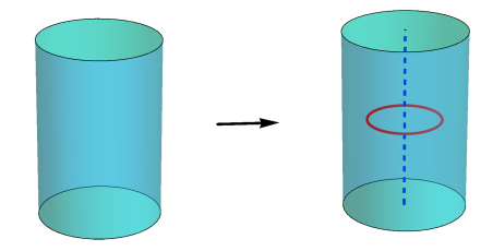
Figure 1: A large gauge transformation produces a Dirac string singularity along the dotted line ${\cal L}$, which is however invisible as any Wilson loop encircling it along ${\cal C}$ is trivial.

These topological sectors are responsible for extending the chiral algebra from a $u(1)$ current algebra to ${\cal A}_{k}$, in particular the currents $W^{\pm}$ correspond to $n=\pm 1$. To see this, we make the standard reduction of $U(1)$ Chern-Simons theory to a chiral boson on the boundary cylinder Moore:1989yh ; Elitzur:1989nr . We start by imposing the following boundary condition on the cylinder $\mathbb{R}\times S^{1}$:

$${A_{-}}_{|\mathbb{R}\times S^{1}}=0.$$ (91)

where $x_{\pm}\equiv\phi\pm t$. Upon partially integrating, the time component $A_{t}$ becomes a Lagrange multiplier for the first-class constraint

$$F_{ij}=0,$$ (92)

where $i,j=1,2$ are components on the disk $D$. Solving the constraint as

$$A_{i}=\partial_{i}\Lambda,$$ (93)

where $\Lambda\sim\Lambda+2\pi$, the action, including the boundary term coming from the above partial integration, reduces to the Floreanini-Jackiw action Floreanini:1987as for a chiral scalar on the boundary,

$$S=-{k\over\pi}\int_{\mathbb{R}\times S^{1}}d^{2}x\partial_{\phi}\Lambda\partial_{-}\Lambda$$ (94)

The conserved energy and $\phi$-momentum are

$$H=P={k\over 2\pi}\int_{S^{1}}d\phi(\partial_{\phi}\Lambda)^{2}.$$ (95)

The solitonic sectors discussed above correspond to winding solutions where

$$\Lambda=n\phi,\qquad n\in\mathbb{Z}.$$ (96)

These carry the conserved charges

$$\Delta:={1\over 2}(H+P)=kn^{2},\qquad\bar{\Delta}:={1\over 2}(H-P)=0,$$ (97)

and therefore, for $n=\pm 1$, they carry the quantum numbers of the chiral currents $W^{\pm}$. A similar analysis of the second $U(1)$ theory leads to the antiholomorphic currents $\overline{W^{\pm}}$. The analysis of Moore:1989yh ; Elitzur:1989nr shows that canonical quantization yields the Hilbert space ${\cal H}_{\mathbb{R}\times D}$ on the solid cylinder to be the vacuum module of ${\cal A}_{k}\times\overline{\cal A}_{k}$.

5.2 Path integral on the solid torus

Next we discuss the path integral of the Chern-Simons theory (87) on thermal AdS₃ whose conformal compactification is a solid torus, ${\cal M}=S^{1}\times D$. From our discussion of the Hilbert space on the solid cylinder one would expect that the result should be the ${\cal A}_{k}\times\overline{\cal A}_{k}$ vacuum character,

$$Z_{S^{1}\times D}\stackrel{{\scriptstyle?}}{{=}}{\rm tr}_{{\cal H}_{\mathbb{R}\times D}}q^{\Delta}\bar{q}^{\bar{\Delta}}=|\chi_{0,k}|^{2},$$ (98)

where $q=e^{2\pi i\tau}$ and $\tau$ the modular parameter of the boundary torus. A small extension of standard results Porrati:2019knx , including the contributions from soliton sectors, shows that this is indeed the case, and we include it here for completeness. As above we make use of the reformulation as a boundary chiral boson theory, though presumably one could also give a more direct bulk computation along the lines of Porrati:2019knx ; Maloney:2020nni .

We focus on the path integral for the first $U(1)$ field $A$. It can be shown Elitzur:1989nr that it reduces to a path integral over the boundary field $\Lambda$ with action (94) without any Jacobian factors. To improve the convergence properties we define the integral through analytic continuation to imaginary time

$$t\rightarrow it_{E}.$$ (99)

We now want to compute the path integral

$$Z^{U(1)}_{{\cal M}}=\int{[D\Lambda]\over V_{\rm gauge}}e^{-S_{E}[\Lambda]},\qquad S_{E}[\Lambda]={k\over\pi}\int_{\delta{\cal M}}\Lambda^{\prime}\partial_{\bar{w}}\Lambda,$$ (100)

where $w:=\phi+it_{E}$. The division by the volume $V_{\rm gauge}$ arises because the action has a restricted gauge invariance

$$\Lambda\rightarrow\Lambda+\alpha(t_{E}).$$ (101)

The boundary $\delta{\cal M}$ in (100) is taken to a torus with complex structure parameter $\tau$, as reflected in the periodicities

$$(t_{E},\phi)\sim(t_{E},\phi+2\pi)\sim(t_{E}+2\pi\tau_{2},\phi+2\pi\tau_{1}).$$ (102)

As argued in the previous subsection, we should allow winding sectors around the $\phi$-circle. It seems natural to also allow winding sectors around the Euclidean time circle, though as we will presently see these do not contribute to the path integral. In the sector with winding numbers $n$ and $m$ around the respective cycles the boundary conditions on the field $\Lambda$ are

$$\Lambda(t_{E},\phi+2\pi) = \Lambda(t_{E},\phi)+2\pi n,$$ (103)

$$\Lambda(t_{E}+2\pi\tau_{2},\phi+2\pi\tau_{1}) = \Lambda(t_{E},\phi)+2\pi m.$$ (104)

The classical solution obeying these boundary conditions is

$$\Lambda_{\rm cl}=n\phi+{m-n\tau_{1}\over\tau_{2}}t_{E},$$ (105)

on which the action takes the value

$$S_{E,\rm cl}=-2\pi ikn(n\tau-m).$$ (106)

We note from (105) that the winding number $m$ can be removed by a large gauge transformation of the type (101) and from (106) that it does not contribute to $e^{-S_{E,\rm cl}}$. The sum over winding sectors labelled by $m$ therefore contributes an $\tau$-independent (infinite) normalization factor, which cancels against a similar factor in $V_{\rm gauge}$.

We expand the field around the classical solution as

$$\Lambda=\Lambda_{\rm cl}+k^{-{1\over 2}}\psi,$$ (107)

where $\psi$ is single-valued on the boundary torus, i.e. it satisfies (104) with $n=m=0$. Performing the gaussian integral over $\psi$ and summing over the winding sectors leads to

$$Z^{U(1)}_{{\cal M}}=\left(\det\,^{\prime}(-\partial_{\phi}\partial_{\bar{w}})\right)^{-{1\over 2}}\sum_{\nu\in\mathbb{Z}}q^{kn^{2}}.$$ (108)

Here the prime on the determinant that it excludes the $\phi$-independent zero modes, which cancel with $V_{\rm gauge}$ in (100). The regularized functional determinant can be computed with standard methods, see e.g. Appendix A of Porrati:2019knx , and equals $\eta^{-1}$. Therefore the path integral leads to the ${\cal A}_{k}$ vacuum character

$$Z^{U(1)}_{{\cal M}}={1\over\eta}\sum_{\nu\in\mathbb{Z}}q^{kn^{2}}=\chi_{0,k}.$$ (109)

Similarly the path integral in the $U(1)_{-k}$ theory leads to $\overline{\chi_{0,k}}$ and combining the two we arrive at (86).

5.3 The sum over topologies

Since the boundary description of the $U(1)_{k}\times U(1)_{-k}$ Cherns-Simons theory includes a stress tensor, constructed as a bilinear in the $u(1)$ current, $T=:J^{2}:$, the theory can be thought of as including gravity in some sense. As such, a nonperturbative definition would involve summing over topologies in the path integral. However, since the Virasoro central charge is one, the gravity sector is strongly coupled and we have no semiclassical control over the topologies we should include, and the prescription is necessarily ad hoc. In the case of a genus-one boundary, a natural family of topologies to include is the $PSL(2,\mathbb{Z})$ family of Euclidean BTZ solutions encountered in semiclassical gravity Maldacena:1998bw . With this assumption, the bulk path integral leads to the Poincaré sum (2) which was our starting point.

6 Comment on multiple boundaries and wormholes

So far we have argued that the path integral of an exotic bulk $U(1)_{k}\times U(1)_{-k}$ theory over manifolds with a genus one boundary yields an ensemble averaged partition function over rational torus CFTs. To extend these observations into a bona fide holographic duality one should in principle show that all observables computed in the bulk reduce to CFT observables in the same weighted ensemble average of theories. Examples of such observables are path integrals in the presence of multiple and/or higher genus boundaries.

Here, we will comment on the path integral with multiple genus one boundaries, which was already studied in the context of ensemble holography for rational CFTs in Meruliya:2021utr . The bulk path integral should contain wormhole-like contributions from geometries which connect several boundary components and whose value is severely constrained by consistency. We want to illustrate how these consistency conditions simplify in ensemble averages where all CFTs have equal weights, as is the case in the primitive ${\cal A}_{k}$ theories. In particular, we will derive an analytic expression for the wormhole contributions when the ensemble contains two CFTs with equal ensemble weights. This happens for our exotic $U(1)_{k}\times U(1)_{-k}$ theory at $k=pq$, where $p$ and $q$ are nonequal primes.

Let us denote by $Z_{1}(\tau),Z_{2}(\tau)$ the torus partition functions of the two CFTs, so that the gravity path integral on a manifold with a single torus boundary is

$$Z^{(1)}_{\rm grav}(\tau_{1})={1\over 2}\Big{(}Z_{1}(\tau)+Z_{2}(\tau)\Big{)}$$ (110)

In the presence of $b$ boundary components with modular parameters $\tau_{i},i=1,\ldots,b$, we will denote by $Z^{(b)}_{\rm grav}(\tau_{1},\ldots,\tau_{b})$ the total bulk path integral and by $Z^{(b)}_{\rm conn}(\tau_{1},\ldots,\tau_{b})$ its connected part, coming (for $b>1$) from wormhole-like geometries which connect all the boundaries. The total path integral should arise from combining the various connected contributions, for example for $b=1,2,3$ we have

$$Z^{(1)}_{\rm grav}(\tau_{1}) = Z^{(1)}_{\rm conn}(\tau_{1})$$ (111)

$$Z^{(2)}_{\rm grav}(\tau_{1},\tau_{2}) = Z^{(1)}_{\rm conn}(\tau_{1})Z^{(1)}_{\rm conn}(\tau_{2})+Z^{(2)}_{\rm conn}(\tau_{1},\tau_{2})$$

$${}Z^{(3)}_{\rm grav}(\tau_{1},\tau_{2},\tau_{3}) = Z^{(1)}_{\rm conn}(\tau_{1})Z^{(1)}_{\rm conn}(\tau_{2})Z^{(1)}_{\rm conn}(\tau_{3})$$ (112)

$$+ Z^{(2)}_{\rm conn}(\tau_{1},\tau_{2})Z^{(1)}_{\rm conn}(\tau_{3})+Z^{(2)}_{\rm conn}(\tau_{1},\tau_{3})Z^{(1)}_{\rm conn}(\tau_{2})+Z^{(2)}_{\rm conn}(\tau_{2},\tau_{3})Z^{(1)}_{\rm conn}(\tau_{1})$$

$$+ Z^{(3)}_{\rm conn}(\tau_{1},\tau_{2},\tau_{3})$$

On the other hand, for consistency of the ensemble interpretation, the gravity path integral with $b$ boundaries should also be equal to an ensemble average with equal weights, namely

$$Z^{(b)}_{\rm grav}(\tau_{1},\ldots,\tau_{b})={1\over 2}\Big{(}Z_{1}(\tau_{1})\ldots Z_{1}(\tau_{b})+Z_{2}(\tau_{1})\ldots Z_{2}(\tau_{b})\Big{)}$$ (113)

Comparing with (112) and its generalization to include more boundary components one finds that the $b$-boundary wormhole contribution should be of the form

$$Z^{(b)}_{\rm conn}(\tau_{1},\ldots,\tau_{b})=w_{b}\Big{(}Z_{1}(\tau_{1})-Z_{2}(\tau_{1})\Big{)}\ldots\Big{(}Z_{1}(\tau_{b})-Z_{2}(\tau_{b})\Big{)},\qquad{\rm for\ }b>1,$$ (114)

with the first few coefficients $w_{b}$ given by

$$w_{2}={1\over 4},\qquad w_{3}=0,\qquad w_{4}=-{1\over 8}.$$ (115)

A recursion relation for the coefficients $w_{b}$ was derived for arbitrary ensemble weights in Meruliya:2021utr . In our special case of equal ensemble weights we can do better and derive an analytic expression for the $w_{b}$ as follows. The generalization of (112) to arbitrary boundaries can be expressed as a standard relation between connected and non-connected generating functions. It is of the schematic form, suppressing the dependence on the modular parameters,

$$\ln\left(1+\sum_{b=1}^{\infty}{k^{b}Z^{(b)}_{\rm grav}\over b!}\right)=\sum_{b=1}^{\infty}{k^{b}Z^{(b)}_{\rm conn}\over b!},$$ (116)

Substituting (113) in the left-hand side we derive

$$\sum_{b=1}^{\infty}{k^{b}Z^{(b)}_{\rm conn}\over b!}={k\over 2}(Z_{1}+Z_{2})+\ln\cosh{k\over 2}(Z_{1}-Z_{2})$$ (117)

Taylor expanding the right-hand side, one finds the results (111) and (114), where the coefficients $w_{b}$ are given by

$$w_{b}=\left\{\begin{array}[]{ll}{(2^{b}-1)B_{b}\over b}&{\rm for\ }b\ {\rm even}\\ 0&{\rm for\ }b\ {\rm odd}\end{array}\right.$$ (118)

Here, $B_{n}$ is the $n$-th Bernoulli number. One checks that this agrees with (115) for $b=2,3,4$.

7 Outlook

In this note we have studied simple examples of ensemble holography which can be seen as rational CFT versions of the Narain holography proposed in Afkhami-Jeddi:2020ezh ; Maloney:2020nni . It is our hope that these can help shed light on some of the puzzles surrounding the meaning and generality of averaged holography.

One aspect of ensemble holography which is readily illustrated in our examples is that it is a feature of path integrals in low energy effective theories which are not UV complete. This is embodied in the fact that our bulk theory only contained massless gauge fields, leading to a spectrum on global AdS₃ consisting of only the vacuum module,

$$Z_{\rm thermal\ AdS_{3}}=|\chi_{0,k}|^{2}.$$ (119)

The sum over topologies leads to a modular invariant answer (2) which is however agnostic as to the precise UV completion and ends up sampling all UV complete CFTs with the relevant chiral algebra. Once we give more information about UV in the form of the matter content, the ensemble of CFTs sampled in the result narrows down Maloney:2020nni . The extreme case of this is if we would add matter fields in the bulk which fill out a modular invariant spectrum, for example leading to the diagonal invariant

$$Z_{\rm thermal\ AdS_{3}}=|\chi_{0,k}|^{2}+2\sum_{\lambda=1}^{k-1}|\chi_{\lambda,k}|^{2}+|\chi_{k,k}|^{2}.$$ (120)

Then the sum over bulk topologies and the corresponding modular average is trivial and doesn’t lead to an ensemble average. Similarly, other UV-complete theories such as the tensionless string on AdS₃ Eberhardt:2018ouy ; Eberhardt:2020bgq and the limit of W_N minimal models dual to 3D vasiliev theory Gaberdiel:2012uj , have modular invariant spectra on global AdS₃.

We end by listing some generalizations and open problems.

• It should be straightforward yet interesting to generalize our examples to rational CFTs involving several bosons on an even integral lattice.

• In sections 3 and 4 we saw that the formula for the ensemble weights drastically simplifies thanks to an additional (semi)group structure on the space of modular invariants. It would be interesting explore such structures and their consequences for ensemble holography in rational Virasoro or Kac-Moody CFTs. Also, it would be satisfying to give an interpretation of the number-theoretic formula (77) for the ensemble weights in terms of CFT data.

• As we illustrated in section 6, the wormhole-like contributions in the presence of multiple boundaries are fixed by consistency and fully calculable in some cases. It would be very interesting to have bulk derivation of these contributions, perhaps along the lines of the results Cotler:2020ugk ; Cotler:2020hgz in pure gravity.

• In order to give a semiclassical justification for the geometries included in the path integral, it would be useful to have simple examples of averaged holography where the gravity sector is weakly coupled, i.e. where the Virasoro central charge is parametrically large (rather than equal to one as in the current work). By a spectral flow operation on the ${\cal A}_{k}$ algebra one can obtain a closely related algebra where Virasoro central charge is large and negative, and which we argued in our previous work Raeymaekers:2020gtz to govern a nonstandard semiclassical limit of pure gravity. It seems likely that the current results can be reinterpreted as a version of ensemble holography for pure gravity in this limit, and we hope to report on this in the near future.

Appendix A Some number-theoretic lemmas

In this Appendix we prove some properties which follow from elementary number theory (see e.g. niven1991introduction ) and which are needed in section 4.

A.1 Semigroup property of modular matrices

We would like to prove the multiplication property (68): for $\alpha,\beta$ square divisors of $k$ and for any $\omega\in G^{\alpha}$ and $\tilde{\omega}\in G^{\beta}$,

$$I^{\alpha}_{\omega}I^{\beta}_{\tilde{\omega}}=I^{[\alpha,\beta]}_{\omega\bullet\tilde{\omega}},$$ (121)

where $\omega\bullet\tilde{\omega}=[\omega\tilde{\omega}]_{2k/[\alpha,\beta]^{2}}$. Since, by definition, $I^{\alpha}_{\omega}=I^{\alpha}_{[\omega]_{2k/\alpha^{2}}}$, we can write (121) more simply as

$$I^{\alpha}_{\omega}I^{\beta}_{\tilde{\omega}}=I^{[\alpha,\beta]}_{\omega\tilde{\omega}}\qquad(\omega\in G^{\alpha},\tilde{\omega}\in G^{\beta}).$$ (122)

We will first show that the property holds for the matrices $M^{\alpha}_{\omega}$ defined in (26), i.e.

$$M^{\alpha}_{\omega}M^{\beta}_{\tilde{\omega}}=M^{[\alpha,\beta]}_{\omega\tilde{\omega}}\qquad(\omega\in G^{\alpha},\tilde{\omega}\in G^{\beta}).$$ (123)

If $\alpha|\nu$ and $\beta|\nu^{\prime}$ then the component expression (27) gives

$$\left(M^{\alpha}_{\omega}M^{\beta}_{\tilde{\omega}}\right)_{\nu\nu^{\prime}}=(\alpha\beta)^{-1}\times\left|\left\{x\in\mathbb{Z}_{2k},\left\{\begin{array}[]{c}x\equiv\omega\nu({\rm mod\ }{2k\over\alpha})\\ x\equiv\tilde{\omega}\nu^{\prime}({\rm mod\ }{2k\over\beta})\end{array}\right.\right\}\right|$$ (124)

The generalization of the Chinese remainder theorem to non-coprime moduli tells us that the simultaneous congruence in the brackets on the right-hand side has solutions if and only if

$$\omega\nu\equiv\tilde{\omega}\nu^{\prime}\left({\rm mod\ }\left({2k\over\alpha},{2k\over\beta}\right)\right).$$ (125)

Note that the modulus in this equation can be written as $\left({2k\over\alpha},{2k\over\beta}\right)={2k\over[\alpha,\beta]}$. One shows that, since $\alpha|\nu$ and $\beta|\nu^{\prime}$, (125) implies that $[\alpha,\beta]$ divides both $\nu$ and $\nu^{\prime}$. Using that $(\omega,{2k\over[\alpha,\beta]^{2}})=1$, we can multiply both sides of (125) by $\omega$ to find the equivalent statement

$$\nu\equiv\omega\tilde{\omega}\nu^{\prime}\left({\rm mod\ }{2k\over[\alpha,\beta]}.\right)$$ (126)

If this is satisfied, the solution is unique modulo $\left[{2k\over\alpha},{2k\over\beta}\right]={2k[\alpha,\beta]\over\alpha\beta}$. The number of solutions of the congruence in $\mathbb{Z}_{2k}$ then equals ${\alpha\beta\over[\alpha,\beta]}$. Equation (124) then becomes

$$\left(M^{\alpha}_{\omega}M^{\beta}_{\tilde{\omega}}\right)_{\nu\nu^{\prime}} = \left\{\begin{array}[]{c l}{1\over[\alpha,\beta]}\delta_{[\nu-\omega\tilde{\omega}\nu^{\prime}]_{2k/[\alpha,\beta]}}&{\rm if\ }[\alpha,\beta]|\nu\ {\rm and\ }[\alpha,\beta]|\nu^{\prime}\\ 0&{\rm otherwise}\end{array}\right.$$ (129)

$$:= \left(M^{[\alpha,\beta]}_{\omega\tilde{\omega}}\right)_{\nu\nu^{\prime}}$$ (130)

From this property one derives the analogous multiplication property (122) for the matrices $I^{\alpha}_{\omega}$ using the relations (31) and (29). Let us illustrate how this works for the $0i$ component of (122), where $i=1,\ldots,k-1$:

$$\left(I^{\alpha}_{\omega}I^{\beta}_{\tilde{\omega}}\right)_{0i} = \big{(}I^{\alpha}_{\omega}\big{)}_{00}\big{(}I^{\beta}_{\tilde{\omega}}\big{)}_{0i}+\big{(}I^{\alpha}_{\omega}\big{)}_{0j}\big{(}I^{\beta}_{\tilde{\omega}}\big{)}_{ji}+\big{(}I^{\alpha}_{\omega}\big{)}_{0k}\big{(}I^{\beta}_{\tilde{\omega}}\big{)}_{ki},\qquad\qquad j=1,\ldots,k-1$$

$$= \sqrt{2}\left(\big{(}M^{\alpha}_{\omega}\big{)}_{00}\big{(}M^{\beta}_{\tilde{\omega}}\big{)}_{0i}+\big{(}M^{\alpha}_{\omega}\big{)}_{0j}\left(\big{(}M^{\beta}_{\tilde{\omega}}\big{)}_{ji}+\big{(}M^{\beta}_{-\tilde{\omega}}\big{)}_{ji}\right)+\big{(}M^{\alpha}_{\omega}\big{)}_{0k}\big{(}M^{\beta}_{\tilde{\omega}}\big{)}_{ki}\right)$$

$$= \sqrt{2}\left(\big{(}M^{\alpha}_{\omega}\big{)}_{00}\big{(}M^{\beta}_{\tilde{\omega}}\big{)}_{0i}+\big{(}M^{\alpha}_{\omega}\big{)}_{0j}\big{(}M^{\beta}_{\tilde{\omega}}\big{)}_{ji}+\big{(}M^{\alpha}_{\omega}\big{)}_{02k-j}\big{(}M^{\beta}_{\tilde{\omega}}\big{)}_{2k-ji}+\big{(}M^{\alpha}_{\omega}\big{)}_{0k}\big{(}M^{\beta}_{\tilde{\omega}}\big{)}_{ki}\right)$$

$$= \sqrt{2}\left(M^{[\alpha,\beta]}_{\omega\tilde{\omega}}\right)_{0i}$$

$$= \left(I^{[\alpha,\beta]}_{\omega\tilde{\omega}}\right)_{0i}.$$

The equality for the other components is proven in a similar manner.

A.2 Maps between the groups $G^{\alpha}$

Next we turn to the proof of the property surrounding eqs. (75,76). Let us consider two quadratic divisors $\alpha$ and $\beta$ of $k$, such that $\beta|\alpha$. Then we have a map from the group $\tilde{G}^{\beta}$ to the group $\tilde{G}^{\alpha}$ provided by

$$\tilde{G}^{\beta}\rightarrow\tilde{G}^{\alpha},\qquad\omega\mapsto[\omega]_{2k/\alpha^{2}}.$$ (131)

We want to show that this map is $N$-to-one, where

$$N={|\tilde{G}^{(\beta)}|\over|\tilde{G}^{(\alpha)}|}=2^{\Omega(k/\beta^{2})-\Omega(k/\alpha^{2})}.$$ (132)

Since the map (131) commutes with multiplication by $-1$, the property also holds for the map between the quotient groups $G^{\alpha}=\tilde{G}^{\alpha}/\{\pm 1\}$ and $G^{\beta}=\tilde{G}^{\beta}/\{\pm 1\}$.

To prove the property, we observe that by redefining $k\rightarrow k/b^{2}$ and $\alpha\rightarrow[\alpha,\beta]$ we can restrict our attention to the case $\beta=1$. Let us choose an arbitrary element $\tilde{\omega}\in G^{\alpha}$. We need to show that the pre-image of $\tilde{\omega}$ under the map (131) consists of precisely $N$ elements, independent of the chosen $\tilde{\omega}$. We recall from section 2.3 that $\tilde{\omega}$ is uniquely defined by a divisor $\tilde{\delta}$ of $k$ satisfying $(\tilde{\delta},k/\tilde{\delta})=\alpha$. More precisely, given a pair of numbers $\tilde{r},\tilde{s}$ from Bezout’s lemma such that

$$\tilde{r}\tilde{\delta}-\tilde{s}k/\tilde{\delta}=\alpha,$$ (133)

$\tilde{\omega}$ can be written as

$$\tilde{\omega}=\left[\tilde{r}{\tilde{\delta}\over\alpha}+\tilde{s}{k\over\alpha\tilde{\delta}}\right]_{2k\over\alpha^{2}}.$$ (134)

The numbers $\tilde{r},\tilde{s}$ are not unique but the class $\tilde{\omega}$ does not depend on which ones we choose. Our property will follow from choosing $\tilde{r},\tilde{s}$ in a judicious way.

To do so, we first decompose $\alpha$ and $k$ in prime factors,

$$\alpha = p_{1}^{a_{1}}\ldots p_{n}^{a_{n}}$$ (135)

$$k = p_{1}^{2a_{1}}\ldots p_{t}^{2a_{t}}p_{t+1}^{2a_{t+1}+c_{t+1}}\ldots p_{n}^{2a_{n}+c_{n}}p_{n+1}^{d_{n+1}}\ldots p_{m}^{d_{m}}$$ (136)

Here, $t$ is by definition smaller than or equal to $n$, and where $t<n$ the numbers $c_{i},i=t+1,\ldots n$ are defined to be strictly positive. Some reflection shows that the integers $m,n$ and $t$ have the interpretation

$$m=\Omega(k),\qquad n=\Omega(\alpha),\qquad t=\Omega(k)-\Omega(k/\alpha^{2}).$$ (137)

The divisor $\tilde{\delta}$ is of the form

$$\tilde{\delta}=p_{1}^{a_{1}}\ldots p_{t}^{a_{t}}p_{N+1}^{a_{t+1}+\tilde{b}_{t+1}c_{t+1}}\ldots p_{n}^{a_{n}+\tilde{b}_{n}c_{n}}p_{n+1}^{\tilde{b}_{n+1}d_{n+1}}\ldots p_{m}^{\tilde{b}_{m}d_{m}}.$$ (138)

It is specified by the numbers $\tilde{b}_{t+1},\ldots\tilde{b}_{n}$ which take the value zero or one.

On the other hand, the elements of $\tilde{G}^{1}$ are in one-to-one correspondence with divisors $\delta$ with $(\delta,k/\delta)=1$. These are of the general form

$$\delta=p_{1}^{2b_{1}a_{1}}\ldots p_{t}^{2b_{t}a_{t}}p_{t+1}^{b_{t+1}(2a_{t+1}+c_{t+1})}\ldots p_{n}^{b_{n}(2a_{n}+c_{n})}p_{n+1}^{b_{n+1}d_{n+1}}\ldots p_{m}^{b_{m}d_{m}},$$ (139)

where $b_{1},\ldots b_{m}$ are either zero or one.

To our specific $\tilde{\delta}$, specified by $\tilde{b}_{t+1},\ldots\tilde{b}_{n}$, we now associate $N=2^{t}$ different divisors $\delta$ of the form

$$\delta=p_{1}^{2b_{1}a_{1}}\ldots p_{t}^{2b_{t}a_{t}}p_{t+1}^{\tilde{b}_{t+1}(2a_{t+1}+c_{t+1})}\ldots p_{n}^{\tilde{b}_{n}(2a_{n}+c_{n})}p_{n+1}^{\tilde{b}_{n+1}d_{n+1}}\ldots p_{m}^{\tilde{b}_{m}d_{m}}.$$ (140)

Here, each $b_{i},i=1,\ldots t$ can take the value zero or one, leading indeed to $2^{t}$ possibilities.

Our property follows if we can show that, for each choice of $\delta$ of the form (140), the associated $\omega_{\delta}$ satisfies

$$\left[\omega_{\delta}\right]_{2k\over\alpha^{2}}=\tilde{\omega}.$$ (141)

First, we rewrite $\delta$ as

$$\delta={\tilde{\delta}\over\alpha}V$$ (142)

where

$$V=p_{1}^{2b_{1}a_{1}}\ldots p_{t}^{2b_{t}a_{t}}p_{t+1}^{\tilde{2}b_{t+1}a_{t+1}}\ldots p_{n}^{2\tilde{b}_{n}2a_{n}}$$ (143)

We note that

$$V|\alpha^{2}.$$ (144)

Now we pick some $r,s$ such that

$$1 = r\delta-s{k\over\delta}$$ (145)

$$= rV{\tilde{\delta}\over\alpha}-s{\alpha^{2}\over V}{k\over\alpha\tilde{\delta}}.$$ (146)

We then choose $\tilde{r},\tilde{s}$ satisfying (133) as follows

$$\tilde{r}=rV,\qquad\tilde{s}=s{\alpha^{2}\over V},$$ (147)

the latter being integer thanks to (144). With this choice equation (134) becomes

$$\tilde{\omega} = \left[r\delta+s{k\over\delta}\right]_{2k\over\alpha^{2}}$$ (148)

$$= \left[\omega_{\delta}\right]_{2k\over\alpha^{2}},$$ (149)

for each of the $N$ choices for $\delta$.

References

- (1) G. Penington, S. H. Shenker, D. Stanford, and Z. Yang, “Replica wormholes and the black hole interior,” arXiv:1911.11977 [hep-th].
- (2) A. Almheiri, T. Hartman, J. Maldacena, E. Shaghoulian, and A. Tajdini, “Replica Wormholes and the Entropy of Hawking Radiation,” JHEP 05 (2020) 013, arXiv:1911.12333 [hep-th].
- (3) C. Teitelboim, “SUPERGRAVITY AND HAMILTONIAN STRUCTURE IN TWO SPACE-TIME DIMENSIONS,” Phys. Lett. B 126 (1983) 46–48.
- (4) R. Jackiw, “Lower Dimensional Gravity,” Nucl. Phys. B 252 (1985) 343–356.
- (5) P. Saad, S. H. Shenker, and D. Stanford, “JT gravity as a matrix integral,” arXiv:1903.11115 [hep-th].
- (6) A. Maloney and E. Witten, “Quantum Gravity Partition Functions in Three Dimensions,” JHEP 02 (2010) 029, arXiv:0712.0155 [hep-th].
- (7) C. A. Keller and A. Maloney, “Poincare Series, 3D Gravity and CFT Spectroscopy,” JHEP 02 (2015) 080, arXiv:1407.6008 [hep-th].
- (8) N. Benjamin, H. Ooguri, S.-H. Shao, and Y. Wang, “Light-cone modular bootstrap and pure gravity,” Phys. Rev. D 100 no. 6, (2019) 066029, arXiv:1906.04184 [hep-th].
- (9) N. Benjamin, S. Collier, and A. Maloney, “Pure Gravity and Conical Defects,” JHEP 09 (2020) 034, arXiv:2004.14428 [hep-th].
- (10) H. Maxfield and G. J. Turiaci, “The path integral of 3D gravity near extremality; or, JT gravity with defects as a matrix integral,” JHEP 01 (2021) 118, arXiv:2006.11317 [hep-th].
- (11) N. Afkhami-Jeddi, H. Cohn, T. Hartman, and A. Tajdini, “Free partition functions and an averaged holographic duality,” JHEP 01 (2021) 130, arXiv:2006.04839 [hep-th].
- (12) A. Maloney and E. Witten, “Averaging over Narain moduli space,” JHEP 10 (2020) 187, arXiv:2006.04855 [hep-th].
- (13) A. Pérez and R. Troncoso, “Gravitational dual of averaged free CFT’s over the Narain lattice,” JHEP 11 (2020) 015, arXiv:2006.08216 [hep-th].
- (14) A. Dymarsky and A. Shapere, “Comments on the holographic description of Narain theories,” arXiv:2012.15830 [hep-th].
- (15) S. Datta, S. Duary, P. Kraus, P. Maity, and A. Maloney, “Adding Flavor to the Narain Ensemble,” arXiv:2102.12509 [hep-th].
- (16) N. Benjamin, C. A. Keller, H. Ooguri, and I. G. Zadeh, “Narain to Narnia,” arXiv:2103.15826 [hep-th].
- (17) M. Ashwinkumar, M. Dodelson, A. Kidambi, J. M. Leedom, and M. Yamazaki, “Chern-Simons Invariants from Ensemble Averages,” arXiv:2104.14710 [hep-th].
- (18) J. Dong, T. Hartman, and Y. Jiang, “Averaging over moduli in deformed WZW models,” arXiv:2105.12594 [hep-th].
- (19) S. Collier and A. Maloney, “Wormholes and Spectral Statistics in the Narain Ensemble,” arXiv:2106.12760 [hep-th].
- (20) N. Benjamin, S. Collier, A. L. Fitzpatrick, A. Maloney, and E. Perlmutter, “Harmonic analysis of 2d CFT partition functions,” arXiv:2107.10744 [hep-th].
- (21) E. Witten, “Quantum Field Theory and the Jones Polynomial,” Commun. Math. Phys. 121 (1989) 351–399.
- (22) G. W. Moore and N. Seiberg, “Taming the Conformal Zoo,” Phys. Lett. B 220 (1989) 422–430.
- (23) S. Elitzur, G. W. Moore, A. Schwimmer, and N. Seiberg, “Remarks on the Canonical Quantization of the Chern-Simons-Witten Theory,” Nucl. Phys. B 326 (1989) 108–134.
- (24) A. Castro, M. R. Gaberdiel, T. Hartman, A. Maloney, and R. Volpato, “The Gravity Dual of the Ising Model,” Phys. Rev. D 85 (2012) 024032, arXiv:1111.1987 [hep-th].
- (25) V. Meruliya, S. Mukhi, and P. Singh, “Poincaré Series, 3d Gravity and Averages of Rational CFT,” JHEP 04 (2021) 267, arXiv:2102.03136 [hep-th].
- (26) V. Meruliya and S. Mukhi, “AdS3 Gravity and RCFT Ensembles with Multiple Invariants,” arXiv:2104.10178 [hep-th].
- (27) G. W. Moore and N. Seiberg, “Naturality in Conformal Field Theory,” Nucl. Phys. B 313 (1989) 16–40.
- (28) A. Cappelli, C. Itzykson, and J. B. Zuber, “Modular Invariant Partition Functions in Two-Dimensions,” Nucl. Phys. B 280 (1987) 445–465.
- (29) A. Cappelli, C. Itzykson, and J. B. Zuber, “The ADE Classification of Minimal and A1(1) Conformal Invariant Theories,” Commun. Math. Phys. 113 (1987) 1.
- (30) J. M. Maldacena and A. Strominger, “AdS(3) black holes and a stringy exclusion principle,” JHEP 12 (1998) 005, arXiv:hep-th/9804085.
- (31) J. Polchinski, String theory. Vol. 1: An introduction to the bosonic string. Cambridge Monographs on Mathematical Physics. Cambridge University Press, 12, 2007.
- (32) P. Di Francesco, H. Saleur, and J. B. Zuber, “Modular Invariance in Nonminimal Two-dimensional Conformal Theories,” Nucl. Phys. B 285 (1987) 454.
- (33) E. Witten, “SL(2,Z) action on three-dimensional conformal field theories with Abelian symmetry,” in From Fields to Strings: Circumnavigating Theoretical Physics: A Conference in Tribute to Ian Kogan, pp. 1173–1200. 7, 2003. arXiv:hep-th/0307041.
- (34) R. Floreanini and R. Jackiw, “Selfdual Fields as Charge Density Solitons,” Phys. Rev. Lett. 59 (1987) 1873.
- (35) M. Porrati and C. Yu, “Kac-Moody and Virasoro Characters from the Perturbative Chern-Simons Path Integral,” JHEP 05 (2019) 083, arXiv:1903.05100 [hep-th].
- (36) L. Eberhardt, M. R. Gaberdiel, and R. Gopakumar, “The Worldsheet Dual of the Symmetric Product CFT,” JHEP 04 (2019) 103, arXiv:1812.01007 [hep-th].
- (37) L. Eberhardt, “Partition functions of the tensionless string,” JHEP 03 (2021) 176, arXiv:2008.07533 [hep-th].
- (38) M. R. Gaberdiel and R. Gopakumar, “Minimal Model Holography,” J. Phys. A46 (2013) 214002, arXiv:1207.6697 [hep-th].
- (39) J. Cotler and K. Jensen, “AdS3 gravity and random CFT,” JHEP 04 (2021) 033, arXiv:2006.08648 [hep-th].
- (40) J. Cotler and K. Jensen, “AdS3 wormholes from a modular bootstrap,” JHEP 11 (2020) 058, arXiv:2007.15653 [hep-th].
- (41) J. Raeymaekers, “Conical spaces, modular invariance and holography,” JHEP 03 (2021) 189, arXiv:2012.07934 [hep-th].
- (42) I. Niven, H. Zuckerman, and H. Montgomery, An Introduction to the Theory of Numbers. Wiley, 1991. https://books.google.cz/books?id=V52HIcKguJ4C.