From networked SIS model to the Gompertz function

Abstract

The Gompertz function is one of the most widely used models in the description of growth processes in many different fields. We obtain a networked version of the Gompertz function as a worst-case scenario for the exact solution to the SIS model on networks. This function is shown to be asymptotically equivalent to the classical scalar Gompertz function for sufficiently large times. It proves to be very effective both as an approximate solution of the networked SIS equation within a wide range of the parameters involved and as a fitting curve for the most diverse empirical data. As an instance, we perform some computational experiments, applying this function to the analysis of two real networks of sexual contacts. The numerical results highlight the analogies and the differences between the exact description provided by the SIS model and the upper bound solution proposed here, observing how the latter amplifies some empirically observed behaviors such as the presence of multiple and successive peaks in the contagion curve.

AMS Subject Classification: 92D39; 05C82, 37N25

1 Introduction

The Gompertz function was first introduced by Benjamin Gompertz in 1825 to describe human mortality curves [1]. Formally, a Gompertz curve can be defined as a non-negative real valued function defined on the open interval $0<t<\infty$ [2]:

$$f\left(t\right)=P\exp\left[-Qe^{-Rt}\right],$$ (1)

where $P,Q,R>0$. It can be proved that it is the solution of the differential equation of the form (see [2] for the formal proof):

$$\dot{f}\left(t\right)=\frac{df(t)}{dt}=QRe^{-Rt}f(t).$$ (2)

A point of inflection for the Gompertz curve is the ordered pair $\left(\dfrac{\log Q}{R},\dfrac{P}{e}\right).$ This curve is appropriate to describe many physical, biological and man-made processes, which are characterized by a rapid growth in the early stages and slower decrease in the late ones. For instance, Finch and Pike [3] have examined maximum life span predictions obtained with the Gompertz mortality rate model and observed that in mammals and birds there is a good agreement on the maximum life span predicted by the model and the ones reported for local populations. In biology, the Gompertz model is frequently used to describe the growth of bacteria and cancer cells. In the last case, many studies are reported in the mathematical biology literature (see, for instance, [4, 5, 6]). The justification for using the Gompertzian models in modeling tumor growth was provided by Frenzen and Murray [7]. They proposed two related maturity-time cell kinetics model mechanisms, which at large time evolve to a Gompertz form. More recently, Karin et al. [8] found that senescent cell turnover slows with age which gives an explanation for the Gompertz law. It is plausible that the ubiquity of the Gompertz model is due to its “diffusive” nature. Gutierrez-Jaimez et al. [9] have proposed a new Gompertz-type diffusion process which allows that bounded sigmoidal growth patterns are modeled by time-continuous variables. Another diffusion-like approach was proposed by Li et al. [10].

Recently, it has been discovered that the Gompertz curve is appropriate to describe different growing processes related to the pandemic of COVID-19. For instance, Ramirez-Torres et al. [11] have used it for estimating the number of unreported cases of COVID-19 in a region/country. Conde-Gutierrez et al. [12] have used the Gompertz function for predicting the dynamics of deaths from the pandemics, while Berihuete et al. [13] used Bayesian approaches implementing the Gompertz function to forecast the evolution of the contagious disease and evaluate the success of particular policies in reducing infections. Mandujano Valle [14] also used this function to estimate the total number of infected and deaths by COVID-19 in Brazil and two Brazilian States (Rio de Janeiro and São Paulo). In another work, Ohnichi et al. [15] demonstrated the existence of a universal scaling behavior for the number of cases of COVID-19 in 11 countries using the Gompertz function.

The similarities and differences between the Gompertz and the logistic model have been the topic of much debate [16, 17, 18, 19]. In general, it has been observed that (i) the lack of symmetry of the Gompertz curve, (ii) the fact that its point of inflection occurs earlier than in the logistic, and (iii) that the carrying capacity is reached relatively earlier than in the logistic curve, are advantages in fitting growth data [19]. All in all, it can be concluded that the Gompertz curve is more useful to fit data of some growth processes than the logistic curve. Additionally, there is evidence on the superiority of the Gompertz vs. the logistic curve in fitting empirical data about the disease progression of pathosystems for more than 100 diseases in plants [18], as well as in reproducing COVID-19 data [20].

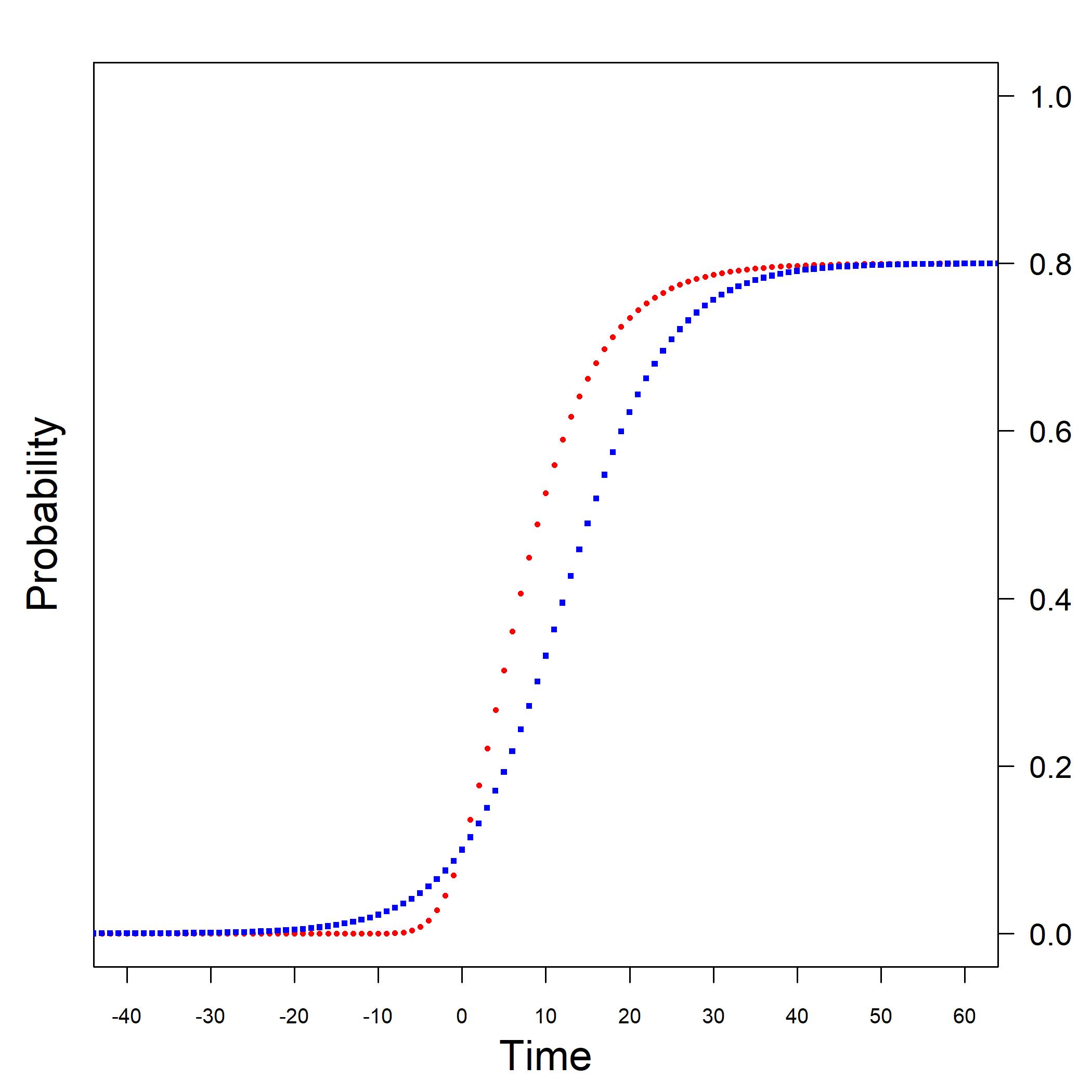
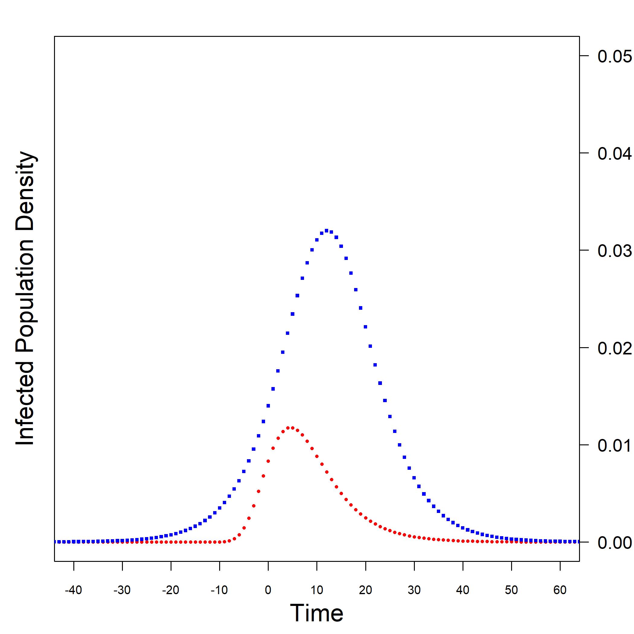
Figure 1: Differences between SIS model (blue square dots plots) and Gompertz model (red circular dots plots). Left panel illustrates the cumulative distribution of the probability to find an infected individual at time $t$ (blue plot is the logistic curve and red plot is the Gompertz curve). Right panel illustrates the infected population density, i.e. the number of individuals who become infected exactly at time $t$, in both models. See the text for explanation and parameters values.

The standard logistic growth curve can be interpreted as the solution of the Susceptible-Infected-Susceptible (SIS) model, the epidemiological model characterized by the possibility of re-infection after recovery (see, for instance, [21] for an up-to-date introduction to the SIS model). In Fig. 1, we illustrate the difference between SIS model and Gompertz model. Blue square dots curves in both boxes refer to the SIS model and red circular dots curves to the Gompertz model. Curves in the left box represent the normalized cumulative number of cases $N(t)$ as a function of time $t$, whereas curves in the right box represent the first derivative $dN(t)/dt$. Curves on the left can be interpreted as the cumulative probabilities to find an infected individual at time $t$ and curves on the right as the probabilities that new individuals get infected at time $t$, or equivalently as the infected population density. All the plots refer to the same set of parameters values. The initial fraction of infected individuals or, more in general, the initial population size is set to $N_{0}=0.1$ and the asymptotic fraction of the infected individuals or, more in general, the final carrying capacity is set to $N_{\infty}=0.8$. In the SIS model, the value of the infection rate is $\beta=0.2$ and the value of the recovering rate is $\gamma=0.04$. Note that, with these values, we have $N_{\infty}=1-\frac{\gamma}{\beta}=0.8$. In the Gompertz model described by Eq. (1), these parameters correspond to $P=N_{\infty}$, $R=\beta\left(1-\frac{\gamma}{\beta}\right)$ and $Q=\log\frac{N_{\infty}}{N_{0}}$, so that, in particular, the value for the damping rate in the Gompertz model is $R=0.16$. Blue lines show the typical symmetrical behavior of the SIS model and of the logistic curve with respect to its inflection point; red lines show the typical asymmetrical behavior and the long tail of the Gompertz model with respect to its inflection point. In fact, the inflection point of the logistic curve is in $N_{\infty}/2=0.4$ at time $t=\frac{1}{R}\log\left(\frac{N_{\infty}}{N_{0}}-1\right)\approx 12.16$, whereas the Gompertz curve is asymmetrical, with an inflection point lower than $N_{\infty}/2$, namely $N=P/e\approx 0.3$ at time $t=\frac{{\log}Q}{R}=\frac{\log\log 8}{0.16}\approx 4.6$. Finally, all plots have been extended to negative times to highlight the complete behavior of the curves.

2 A worst-case scenario SIS model

Let $G=\left(V,E\right)$ be a simple connected graph on $n$ vertices (nodes). We will use indistinctly graph or network to refer to $G$. The networked SIS model is described by the following $n$ equations:

$$\dot{x}_{i}(t)=\beta[1-x_{i}(t)]\sum_{j=1}^{n}A_{ij}x_{j}(t)-\gamma x_{i}(t),$$ (3)

where $x_{i}(t)$ represents the probability that node $i$ is infected at time $t$ and $x_{i}(0)=x_{0i}=p$, $\forall i=1,\dots,n$, for some $0<p<1$, the initial probability of being infected, equal for all nodes. Elements $A_{ij}$ are the corresponding entries of the adjacency matrix $\mathbf{A}$ of $G$. In matrix-vector form, Eq. (3) becomes:

$$\dot{{\bf x}}(t)=\beta\left[{\bf I}-{\rm diag}({\bf x}(t))\right]{\bf A}\,{\bf x}(t)-\gamma{\bf x}(t),$$ (4)

with ${\bf x}=\left[{x_{1}},{x_{2}},\dots,{x_{n}}\right]\in{\mathbb{R}}^{n}$ and ${\bf x}(0)={\bf x}_{0}=p\,{\bf u}$, where ${\bf I}$ is the identity matrix of the corresponding order and ${\bf u}$ the vector whose components are all equal to $1$. In what follows, we write in general ${\bf v}\preceq{\bf w}$ for ${\bf v},{\bf w}\in{\mathbb{R}}^{n}$ if ${v_{i}}\leq{w_{i}},\ \forall i=1,\dots,n$.

Let us now rewrite the networked SIS model on the basis of the information content $I_{i}(t)$ that a given node $i$ is not infected at time $t$. The information content (also known as surprisal, self-information, or Shannon information) is given by

$$I_{i}(t)=-\log[1-x_{i}(t)],\quad\forall i=1,\dots,n,$$ (5)

where $s_{i}\left(t\right)=1-x_{i}(t)$ is the probability of not being infected at time $t$, i.e., of being susceptible. The information content SIS model (IC-SIS) is now written as

$$\dot{I}_{i}(t)=\beta\sum_{j=1}^{n}A_{ij}\left(1-e^{-I_{j}\left(t\right)}\right)-\gamma\sum_{j=1}^{n}\delta_{ij}\left(e^{I_{j}\left(t\right)}-1\right),$$ (6)

with $\delta_{ij}$ being the Kronecker delta and $I_{i}(0)=-\log(1-p)=-\log q$, where $q=1-p$.

Let us consider the function $f(I)=1-e^{-I}$, which is increasingly concave, so that we can write

$$f(I)<f(I_{0})+f^{\prime}(I_{0})(I-I_{0})=e^{-I_{0}}I+1-e^{-I_{0}}(I_{0}+1).$$

Analogously, because $g(I)=e^{I}-1$ is increasingly convex we have

$$g(I)>g(I_{0})+g^{\prime}(I_{0})(I-I_{0})=e^{I_{0}}I-1-e^{I_{0}}(I_{0}-1).$$

Therefore, we have

$$\dot{I}_{i}(t)<\beta\sum_{j=1}^{n}A_{ij}\left[e^{-I_{0}}I_{j}+1-e^{-I_{0}}(I_{0}+1)\right]-\gamma\sum_{j=1}^{n}\delta_{ij}\left[e^{I_{0}}I_{j}-1-e^{I_{0}}(I_{0}-1)\right].$$

Let us call the right-hand-side part of this equation the worst-case scenario IC-SIS as it represents a clear upper bound to the surprisal that a given node $i$ is not infected at time $t$. Let us designate it by $\dot{\hat{I}}_{i}(t)$ and taking into account that $x_{0}=p$, $I_{0}=-\log q$, $e^{-I_{0}}=q$ and $e^{I_{0}}=1/q$, we can write it as

$$\dot{\hat{I}}_{i}(t)=\beta q\sum_{j=1}^{n}A_{ij}\hat{I}_{j}(t)-\frac{\gamma}{q}\sum_{j=1}^{n}\delta_{ij}\hat{I}_{j}(t)+\beta(p+q\log q)\sum_{j=1}^{n}A_{ij}-\gamma\,\frac{p+\log q}{q},$$

where $\hat{I}_{i}(t)$ is the worst-case scenario surprisal that the node $i$ is not infected at time $t$. When written in matrix-vector form

$$\dot{\hat{\mathcal{{\bf\mathscr{I}}}}}(t)=\left(\beta q{\bf A}-\frac{\gamma}{q}{\bf I}\right){\hat{{\bf\mathscr{I}}}}(t)+\left[\beta(p+q\log q){\bf A}-\frac{\gamma}{q}(p+\log q){\bf I}\right]{\bf u},$$ (7)

it is easy to realize that this equation has the linear form

$$\dot{\hat{\mathcal{{\bf\mathscr{I}}}}}(t)={\bf B}{\hat{{\bf\mathscr{I}}}}+{\bf b},$$ (8)

where ${\bf B}\coloneqq q\beta{\bf A}-\frac{\gamma}{q}{\bf I}$ and ${\bf b}\coloneqq\left[(p+q\log q)\beta{\bf A}-(p+\log q)\frac{\gamma}{q}{\bf I}\right]{\bf u}$.

As a way of comparison, we will also consider the “standard” linearization of the SIS model around the point ${\bf 0}$:

$$\dot{\mathbf{x}}\left(t\right)=\left(\beta\mathbf{A}-\gamma\mathbf{I}\right)\mathbf{x}\left(t\right),$$ (9)

with initial condition $\mathbf{x}_{0}$, whose solution is ${\mathbf{\bar{x}}}\left(t\right)=\exp\left[\left(\beta\mathbf{A}-\gamma\mathbf{I}\right)t\right]\mathbf{x}_{0}$. It is easy to realize that this solution is exponentially unstable. We now formally prove that the solution $\mathbf{\hat{x}}\left(t\right)\coloneqq 1-\exp\big{[}-{\hat{{\bf\mathscr{I}}}}\big{]}$ to the worst-case scenario SIS model is an upper bound – therefore a worst-case scenario solution – to the exact SIS model solution, i.e. $\mathbf{x}\left(t\right)\preceq\mathbf{\hat{x}}\left(t\right),$ and that it is a lower bound to the divergent solution of the linearized model, i.e. $\mathbf{\hat{x}}\left(t\right)\preceq{\mathbf{\bar{x}}}\left(t\right)$.

Theorem 1.

Let $\mathbf{x}\left(t\right)$, $\mathbf{\hat{x}}\left(t\right)$ and $\mathbf{\bar{x}}\left(t\right)$ be, respectively, the solution of the exact SIS model in Eq. (4), of the worst-case scenario IC-SIS model obtained from Eq. (7) and of the linearized SIS model in Eq. (9), with the same initial conditions: $\mathbf{x}\left(0\right)=\mathbf{\hat{x}}\left(0\right)={\mathbf{\bar{x}}}\left(0\right)=p\mathbf{u}$. Then, $\forall t\geq 0$,

$$\mathbf{x}\left(t\right)\preceq\mathbf{\hat{x}}\left(t\right)\preceq{\mathbf{\bar{x}}}\left(t\right).$$ (10)

where the second inequality holds if $\beta_{e}\coloneqq\frac{\beta}{\gamma}>\frac{1}{q^{2}k_{\rm min}}$, with $k_{\rm min}$ minimum degree of the graph.

Proof.

We first prove that $\mathbf{x}\left(t\right)\preceq\mathbf{\hat{x}}\left(t\right)$. By the method of variation of parameters, the solution of the worst-case scenario IC-SIS model is

$$\hat{{\bf\mathscr{I}}}(t)=e^{{\bf B}t}\,\mathscr{I}_{0}+\left(e^{{\bf B}t}-{\bf I}\right){\bf B}^{-1}{\bf b},$$ (11)

which is equivalent to

$$\hat{{\bf\mathscr{I}}}(t)=e^{{\bf B}t}\left[{\bf B}^{-1}{\bf b}-\log q\,{\bf u}\right]-{\bf B}^{-1}{\bf b}.$$ (12)

Since $I_{i}(0)=\hat{I}_{i}(0)=-\log q$ and $\dot{I}_{i}(t)<\dot{\hat{I}}_{i}(t),\ \forall t\geq 0$, $\forall i=1,\dots,n$, following Lemma A.1 by Lee et al. [22], p. 11,

$$\hat{x}_{i}(t)=1-e^{-\hat{I}_{i}(0)}.$$ (13)

is an upper bound for the original SIS network model solution ${x}_{i}(t),\forall t\geq 0$, $\forall i=1,\dots,n$, and this proves the first inequality. We now prove that $\mathbf{\hat{x}}\left(t\right)\preceq{\mathbf{\bar{x}}}\left(t\right)$. To this purpose, let us assume that $q\beta k_{\rm min}-\frac{\gamma}{q}>0$, which implies $q\beta\lambda_{1}-\frac{\gamma}{q}>0$, where $\lambda_{1}$ is the eigenvalue corresponding to the dominant eigenvector of $\bf A$. Under this condition, since $q<1$, we have $\beta\lambda_{1}\geq\beta k_{\rm min}>\frac{\gamma}{q^{2}}>\frac{\gamma}{q}>{\gamma}$ and both the solutions of the upper bound problem $\mathbf{\hat{x}}\left(t\right)$ and of the linearized problem ${\mathbf{\bar{x}}}\left(t\right)$ are increasing functions in time. Again, by Lemma A.1 in [22], since the initial conditions are the same for both processes, i.e., $\mathbf{\hat{x}}\left(0\right)={\mathbf{\bar{x}}}\left(0\right)=\mathbf{x}_{0}=p\mathbf{u}$, it is enough to prove that

$$\dfrac{d\mathbf{\hat{x}}\left(t\right)}{dt}\preceq\dfrac{d{\mathbf{\bar{x}}}\left(t\right)}{dt}$$ (14)

for all $t\geq 0$. Being $\mathbf{\hat{x}}\left(t\right)=1-e^{-\mathbf{\hat{\mathscr{I}}}}$, then we have

$$\dfrac{d\mathbf{\hat{x}}\left(t\right)}{dt}=e^{-\mathbf{\hat{\mathscr{I}}}}\dfrac{d\mathbf{\hat{\mathscr{I}}}\left(t\right)}{dt}\preceq\dfrac{d\hat{\mathbf{\mathscr{I}}}\left(t\right)}{dt}$$ (15)

for all $t\geq 0$, where the inequality in Eq. (15) follows from $e^{-{\hat{I}_{i}}}<1$ for all $\hat{I}_{i}\in[0,\infty)$. By Eq. (12) we have

$$\dfrac{d\mathbf{\hat{\mathscr{I}}}\left(t\right)}{dt}=e^{\mathbf{B}t}\mathbf{B}\left[\mathbf{B}^{-1}{\bf b}-\log q\,{\bf u}\right]=e^{\mathbf{B}t}\left[{\bf b}-\log q\,\mathbf{B}{\bf u}\right]$$

where $\mathbf{B}=\beta q\mathbf{A}-\frac{\gamma}{q}\mathbf{I}$ and ${\bf b}=\left[\left(p+q\log q\right)\beta\mathbf{A}-\left(p+\log q\right)\frac{\gamma}{q}\mathbf{I}\right]{\bf u}$. Since

$${\bf b}-\log q\,\mathbf{B}{\bf u}=p\left(\beta\mathbf{A}-\frac{\gamma}{q}\mathbf{I}\right){\bf u}$$

we have

$$\dfrac{d\mathbf{\hat{\mathscr{I}}}\left(t\right)}{dt}=e^{\left(q\beta{\bf A}-\frac{\gamma}{q}{\bf I}\right)t}\left[p\left(\beta{\bf A}-\frac{\gamma}{q}{\bf I}\right){\bf u}\right]\preceq e^{\left(\beta{\bf A}-\gamma{\bf I}\right)t}\left[p\left(\beta{\bf A}-\gamma{\bf I}\right){\bf u}\right]=\dfrac{d{\mathbf{\bar{x}}}\left(t\right)}{dt}.$$ (16)

The last inequality can be justified in the following way. Being $\bf A$ and $\bf I$ commuting matrices, Eq. (16) is equivalent to $e^{q\beta{\bf A}t}e^{-\frac{\gamma}{q}{\bf I}t}\left(\beta{\bf A}-\frac{\gamma}{q}{\bf I}\right){\bf u}\preceq e^{\beta{\bf A}t}e^{-{\gamma}{\bf I}t}\left(\beta{\bf A}-\gamma{\bf I}\right){\bf u}$ and, hence, to the inequality

$$e^{q\beta{\bf A}t}\left(\beta{\bf A}-\frac{\gamma}{q}{\bf I}\right){\bf u}\preceq e^{\frac{p}{q}\gamma t}e^{\beta{\bf A}t}\left(\beta{\bf A}-\gamma{\bf I}\right){\bf u}.$$

Moreover, $q\beta{\bf A}\succeq 0$ and $\beta{\bf A}\succeq 0$, with $q\beta{\bf A}\preceq\beta{\bf A}$ element by element, such that

$${\bf 0}\preceq\left(\beta{\bf A}-\frac{\gamma}{q}{\bf I}\right){\bf u}\preceq\left(\beta{\bf A}-{\gamma}{\bf I}\right){\bf u}$$

where $\bf 0$ is the null vector, since we assume $\beta k_{\rm min}-\frac{\gamma}{q}>0$. Therefore, we have $e^{q\beta{\bf A}t}\left(\beta{\bf A}-\frac{\gamma}{q}{\bf I}\right){\bf u}\preceq e^{\beta{\bf A}t}\left(\beta{\bf A}-\gamma{\bf I}\right){\bf u}$, for all $t\geq 0$ and, being $e^{\beta{\bf A}t}\left(\beta{\bf A}-\gamma{\bf I}\right){\bf u}\preceq e^{\frac{p}{q}\gamma t}e^{\beta{\bf A}t}\left(\beta{\bf A}-\gamma{\bf I}\right){\bf u}$, for all $t\geq 0$, all the components of the vector in the left hand side of Eq. (16) are less than or equal to the corresponding components of the vector in the right hand side. Finally Eq. (15) and Eq. (16) imply Eq. (14) and this ends the proof. ∎

Remark 1.

If $\gamma=0$, we have ${\bf B}=q\beta{\bf A}$ and ${\bf b}=(p+q\log q)\beta{\bf A}{\bf u}$ so that ${\bf B}^{-1}{\bf b}=\left(\frac{p}{q}+\log q\right){\bf u}$. Solution in Eq. (12) reduces to

$$\hat{{\bf\mathscr{I}}}(t)=\frac{p}{q}e^{q\beta{\bf A}t}{\bf u}-\left(\frac{p}{q}+\log q\right){\bf u},$$

and it is equal to the solution for the SI Model by Lee et al. (see [22] and [23]). Let us observe that if $t=0$: $\hat{{\bf\mathscr{I}}}(0)=-\log q\,{\bf u}$ and ${{\bf\hat{x}}}(0)=p$, as expected. Moreover, for $t\to+\infty$, $\hat{{\bf\mathscr{I}}}(t)\to+\infty$ and ${{\bf\hat{x}}}(t)\to{\bf u}$.

Remark 2.

If $\beta=0$, ${\bf B}=-\frac{\gamma}{q}{\bf I}$ and ${\bf b}=-(p+\log q)\frac{\gamma}{q}{\bf u}$ so that ${\bf B}^{-1}{\bf b}=(p+\log q){\bf u}$. Solution in Eq. (12) reduces to

$$\hat{{\bf\mathscr{I}}}(t)=p\left(e^{-\frac{\gamma}{q}t}-1\right){\bf u}-\log q\,{\bf u}.$$

Let us observe that for $t\to+\infty$, $\hat{{\bf\mathscr{I}}}(t)\to-(p+\log q){\bf u}$ and $\hat{{\bf x}}(t)\to(1-qe^{p}){\bf u}$. This bound doesn’t converge to ${\bf x}^{\star}={\bf 0}$ as $t\to+\infty$ but to $(1-qe^{p}){\bf u}$. Observe that $0<1-qe^{p}<p$, as expected, and that $1-qe^{p}\sim p^{2}$ as $p\to 0$.

Remark 3.

Let us consider $\beta\neq 0$ and $\gamma\neq 0$. The exponential term in Eq. (12) may be written as

$$e^{{\bf B}t}=e^{(q\beta{\bf A}-\frac{\gamma}{q}{\bf I})t}=e^{(q\beta{\bf M}{\bf\Lambda}{\bf M}^{T}-\frac{\gamma}{q}{\bf I})t}=e^{{\bf M}(q\beta{\bf\Lambda}-\frac{\gamma}{q}{\bf I}){\bf M}^{T}t}={\bf M}e^{(q\beta{\bf\Lambda}-\frac{\gamma}{q}{\bf I})t}{\bf M}^{T},$$

where ${\bf\Lambda}$ is the diagonal matrix of the eigenvalues of ${\bf A}$ and ${\bf M}$ is the orthogonal matrix whose columns are the eigenvectors of ${\bf A}$. As $t$ grows to $+\infty$, the diagonal exponential terms $e^{(q\beta\lambda_{i}-\frac{\gamma}{q})t}$ grows to $+\infty$ if $(q\beta\lambda_{i}-\frac{\gamma}{q})>0$. In particular, if $(q\beta\lambda_{1}-\frac{\gamma}{q})<0$, no one of these terms grows to $+\infty$ and the epidemic decays. Thus, we can identify a threshold given by the following condition

$$\beta_{e}=\frac{\beta}{\gamma}<\frac{1}{q^{2}\lambda_{1}}\coloneqq\tau,$$ (17)

and we can identify $\tau=\frac{1}{q^{2}\lambda_{1}}$ as the threshold of the worst-case scenario solution. Then, if $\beta_{e}<\tau$ the epidemic decays; if $\beta_{e}>\tau$ the epidemic grows. Let us observe that, as $\lambda_{1}$ increases (and so does the average degree in the network), condition in Eq. (17) becomes stricter and the spread of epidemics is easier; moreover, in general, $\tau$ is greater than $1/\lambda_{1}$ and, as $p$ decreases, it approaches the lower bound $1/\lambda_{1}$.

2.1 Gompertz-like function from SIS

Let us start by defining a matrix ${\bf D}$ as

$${\bf D}\coloneqq{\bf I}-q^{2}\beta_{e}{\bf A},$$ (18)

so that ${\bf B}=-\frac{\gamma}{q}{\bf D}$. Then we can rewrite the vector ${\bf B}^{-1}{\bf b}-\log q\,{\bf u}$ appearing in Eq. (12) in the following way:

$${\bf B}^{-1}{\bf b}-\log q\,{\bf u}=\frac{p}{q}\left[{\bf I}-p({\bf I}-q^{2}\beta_{e}{\bf A})^{-1}\right]{\bf u}=\frac{p}{q}\left[{\bf I}-p{\bf D}^{-1}\right]{\bf u}.$$

In this way, the solution of the worst-case scenario IC-SIS model becomes

$$\hat{{\bf\mathscr{I}}}(t)=\frac{p}{q}\left[e^{-\frac{\gamma}{q}{\bf D}t}-{\bf I}\right]\left[{\bf I}-p{\bf D}^{-1}\right]{\bf u}-\log q\,{\bf u}.$$ (19)

We are now in a position to present the main result of the current work.

Theorem 2.

Let $G$ be a graph in which there is a IC-SIS dynamics taking place on its nodes and edges. Let $\psi_{\nu}\left(i\right)$ be the $i$-th entry of the $\nu$-th (orthonormalized) eigenvector of $\mathbf{A}$, associated with the eigenvalue $\lambda_{\nu}$, with $\lambda_{n}\leq\dots\leq\lambda_{2}\leq\lambda_{1}$. Then, under the condition $\beta_{e}<q\tau$, the worst-case scenario probability $\tilde{s}_{i}(t)$ that a node $i$ is susceptible of getting infected for time $t\rightarrow\infty$ is given by a Gompertz function of the form

$$\tilde{s}_{i}(t)=P_{i}\exp\left[-Q_{i}e^{-Rt}\right]$$ (20)

where $P_{i}=q\exp\left[\sum_{\nu=1}^{n}\alpha_{\nu}\zeta_{\nu}(i)\right]$, $Q_{i}=\alpha_{1}\zeta_{1}(i)$ and $R=\frac{\gamma}{q}(1-q^{2}\beta_{e}\lambda_{1})$ with $\alpha_{\nu}\coloneqq\frac{p-pq\beta_{e}\lambda_{\nu}}{1-q^{2}\beta_{e}\lambda_{\nu}}$ and $\zeta_{\nu}(i)\coloneqq\psi_{\nu}(i)\sum_{j=1}^{n}\psi_{\nu}(j)$, $\forall\nu=1,\dots,n$.

Proof.

Let’s start from Eq. (19)

$$\hat{{\bf\mathscr{I}}}(t)=\frac{p}{q}\left[e^{-\frac{\gamma}{q}{\bf D}t}-{\bf I}\right]\left[{\bf I}-p{\bf D}^{-1}\right]{\bf u}-\log q\,{\bf u}$$

Since ${\bf D}={\bf I}-q^{2}\beta_{e}{\bf A}$ is symmetric and there exists an orthogonal matrix ${\bf M}$ whose columns are the eigenvectors of ${\bf A}$ and, consequently, of ${\bf D}$ such that

$${\bf D}={\bf M}\,{\rm diag}(1-q^{2}\beta_{e}\lambda_{\nu})\,{\bf M}^{T}$$

we have

$$\begin{split}\hat{{\bf\mathscr{I}}}(t)&=\frac{p}{q}{\bf M}\,{\rm diag}\left[\left(e^{-\frac{\gamma}{q}(1-q^{2}\beta_{e}\lambda_{\nu})t}-1\right)\,\left(1-\frac{p}{1-q^{2}\beta_{e}\lambda_{\nu}}\right)\right]{\bf M}^{T}\,{\bf u}-\log q\,{\bf u}\\ &=\frac{p}{q}{\bf M}\,{\rm diag}\left[\frac{q-q^{2}\beta_{e}\lambda_{\nu}}{1-q^{2}\beta_{e}\lambda_{\nu}}\left(e^{-\frac{\gamma}{q}(1-q^{2}\beta_{e}\lambda_{\nu})t}-1\right)\,\right]{\bf M}^{T}\,{\bf u}-\log q\,{\bf u}\\ &={\bf M}\,\Lambda(t){\bf M}^{T}\,{\bf u}-\log q\,{\bf u}\end{split}$$

where $\Lambda(t)={\rm diag}\left[\eta_{\nu}(t)\right]$ and $\eta_{\nu}(t)=\alpha_{\nu}\left(e^{-\frac{\gamma}{q}(1-q^{2}\beta_{e}\lambda_{\nu})t}-1\right)$ with $\alpha_{\nu}\coloneqq\frac{p-pq\beta_{e}\lambda_{\nu}}{1-q^{2}\beta_{e}\lambda_{\nu}}$. Now, since $\hat{{\bf s}}(t)=e^{-\hat{{\bf\mathscr{I}}}(t)}$:

$$\begin{split}\hat{s}_{i}(t)&=q\exp\left[-\left({\bf M}\,\Lambda(t){\bf M}^{T}\,{\bf u}\right)_{i}\right]\\ &=q\exp\left[-\sum_{j=1}^{n}\sum_{\nu=1}^{n}\psi_{\nu}\left(i\right)\psi_{\nu}\left(j\right)\eta_{\nu}(t)\right]\\ &=q\exp\left[-\sum_{\nu=1}^{n}\zeta_{\nu}(i)\eta_{\nu}(t)\right]\\ \end{split}$$

where $\zeta_{\nu}(i)\coloneqq\psi_{\nu}(i)\sum_{j=1}^{n}\psi_{\nu}(j)$. Now, in order to describe the asymptotic behavior of $\hat{s}_{i}(t)$, let us consider separately the following three cases:

1. $\beta_{e}<q\tau$, that is $1-q\beta_{e}\lambda_{1}>0$, which implies $1-q^{2}\beta_{e}\lambda_{1}>0$:

   $$\begin{split}\hat{s}_{i}(t)&=q\exp\left[-\sum_{\nu=1}^{n}\zeta_{\nu}(i)\eta_{\nu}(t)\right]\\ &\sim q\exp\left[-\left(\zeta_{1}(i)\alpha_{1}e^{-\frac{\gamma}{q}(1-q^{2}\beta_{e}\lambda_{1})t}-\sum_{\nu=1}^{n}\zeta_{\nu}(i)\alpha_{\nu}\right)\right]\\ &=q\exp\left[\sum_{\nu=1}^{n}\zeta_{\nu}(i)\alpha_{\nu}\right]\exp\left[-\zeta_{1}(i)\alpha_{1}e^{-\frac{\gamma}{q}(1-q^{2}\beta_{e}\lambda_{1})t}\right]\coloneqq\tilde{s}_{i}(t)\\ \end{split}$$ (21)

   In particular, for $t\to+\infty$

   $$\hat{s}_{i}(t)\to q\exp\left[\sum_{\nu=1}^{n}\zeta_{\nu}(i)\alpha_{\nu}\right]$$

   The last term in Eq. (21) can be interpreted as a Gompertz function. Indeed, it is

   $$\tilde{s}_{i}(t)=P_{i}\exp\left[-Q_{i}e^{-Rt}\right]$$ (22)

   with $P_{i}=q\exp\left[\sum_{\nu=1}^{n}\alpha_{\nu}\zeta_{\nu}(i)\right]$, $Q_{i}=\alpha_{1}\zeta_{1}(i)$ and $R=\frac{\gamma}{q}(1-q^{2}\beta_{e}\lambda_{1})$. Let us observe that $\zeta_{1}(i)=\psi_{1}(i)\sum_{j=1}^{n}\psi_{1}(j)$ is positive $\forall i=1,\dots,n$ as the eigenvector associated to the dominant eigenvalue $\lambda_{1}$ has components all with the same sign. Moreover, in order to get also $Q_{i}>0$, the further condition $1-q\beta_{e}\lambda_{1}>0$, equivalent to $\beta_{e}<q\tau$, must be satisfied. Let us notice that this condition is stricter than $1-q^{2}\beta_{e}\lambda_{1}>0$, which is equivalent to $\beta_{e}<\tau$.

2. $q\tau<\beta_{e}<\tau$: in this case Eq. (21) still holds but it cannot be considered a Gompertz function since $\alpha_{1}<0$.

3. $\beta_{e}>\tau$, that is $1-q^{2}\beta_{e}\lambda_{1}<0$:

   $$\begin{split}\hat{s}_{i}(t)&=q\exp\left[-\sum_{\nu=1}^{n}\zeta_{\nu}(i)\eta_{\nu}(t)\right]\\ &\sim q\exp\left[-\alpha_{1}\zeta_{1}(i)e^{-\frac{\gamma}{q}(1-q^{2}\beta_{e}\lambda_{1})t}\right]\\ \end{split}$$ (23)

   where again $\zeta_{1}(i)>0$ and also $\alpha_{1}=\frac{p-pq\beta_{e}\lambda_{1}}{1-q^{2}\beta_{e}\lambda_{1}}>0$ since now $1-q\beta_{e}\lambda_{1}<0$. Therefore, in this case, we have as expected $\hat{s}_{i}(t)\to 0$ for $t\to+\infty$.

∎

Remark 4.

According to Theorem 2, when the time is sufficiently large, the solution of the worst-case scenario IC-SIS on a network is a Gompertz function of the type: $f\left(t\right)=P\exp\left[{-Qe^{-Rt}}\right]$, under the condition that the effective infectivity rate is lower than $q\tau=\frac{1}{q\lambda_{1}}$. This is an important result because, as we have seen in the Fig. 1, the main differences between the SIS model and the Gompertz model occurs not at early times of the disease propagation but when the time is sufficiently large. Additionally, it is also at large time when the two models developed by Frenzen and Murray [7] coincide with a Gompertz curve, which would open some interesting avenues for future exploration of these models in relation to the current one.

Remark 5.

Let us notice that, according to Eq. (20), the probability density can be written as

$$\frac{d\tilde{s}_{i}(t)}{dt}=\tilde{s}_{i}(t)\left[Q_{i}Re^{-Rt}\right]$$ (24)

and the point of inflection of the Gompertz curve is then given by

$$t=\frac{\log Q_{i}}{R}=\frac{q}{\gamma(1-q^{2}\beta_{e}\lambda_{1})}\log[\alpha_{1}\zeta_{1}(i)]$$ (25)

This inflection point, which is the time at which the probability density of recovering from infection is maximum, grows with the logarithm of $\zeta_{1}(i)$ and $\zeta_{1}(i)$ is proportional to the eigenvector centrality of node $i$. This means that the more central is the node, in terms of eigenvector centrality, the more this maximum is delayed in time and the slower will be the healing process for that node.

Remark 6.

Finally, we conclude by observing that Eq. (19) can be given the following interesting expression. When the effective infectivity rate is below the threshold $\tau$, that is if it is satisfied the condition $0<q^{2}\beta_{e}<\frac{1}{\lambda_{1}}$, the inverse ${\bf D}^{-1}=\left[{\bf I}-q^{2}\beta_{e}{\bf A}\right]^{-1}$ can be considered a matrix resolvent and ${\bf D}^{-1}{\bf u}=\left[{\bf I}-q^{2}\beta_{e}{\bf A}\right]^{-1}{\bf u}={\bf u}+{\bf c}$, where ${\bf c}=\left[\left(\mathbf{I}-q^{2}\beta_{e}\mathbf{A}\right)^{-1}-\mathbf{I}\right]\mathbf{u}$, for $0<q^{2}\beta_{e}<\frac{1}{\lambda_{1}}$, is the vector whose entries are the so-called Katz centrality indices of the nodes in the network [24]. This index belongs to a family of network descriptors which counts the number of walks in the graph involving the corresponding node, giving more weight to the shorter than to the longer ones [25]. Therefore we have

$$\left[{\bf I}-p{\bf D}^{-1}\right]{\bf u}={\bf u}-p{\bf D}^{-1}{\bf u}={\bf u}-p\,{\bf u}-p\,{\bf c}=q\,{\bf u}-p\,{\bf c}.$$

and the upper bound solution of the IC-SIS model in Eq. (19) may be expressed in terms of the Katz centralities of the nodes as

$$\hat{{\bf\mathscr{I}}}(t)=p\left[e^{-\frac{\gamma}{q}{\bf D}t}-{\bf I}\right]\left[{\bf u}-\frac{p}{q}\,{\bf c}\right]-\log q\,{\bf u}.$$ (26)

2.2 Computational experiments

We now present some numerical results from computational experiments carried out on two real-world sexual contact networks. The rationale for choosing networks of this type lies in the fact that they typically host contagion processes that can be described using the SIS model. The spreading of many different epidemics of global interest, like influenza, Ebola, Zika, Chikungunya, and others, has been analyzed by applying this model. For instance, Juher et al. [26] studied in details the Syphilis transmission characteristics and disease evolution on a large sexual network in San Francisco and Zhao et al. [27] investigate, in the same framework, the temporal patterns and transmission potential of ZIKA virus in eight Brazilian states, over the same period.

Here we focus on two specific sexual contact networks. Both networks are connected, unweighted and undirected. The first corresponds to $m=83$ heterosexual contacts between $n=82$ individuals ($35$ males and $47$ females). In this network there is available information about the sex of the individuals. The network was studied in details in [28] where a subset of individuals were infected with Chlamydia Trachomatis and/or Neisseria Gonorrhoeae in Manitoba, Canada. We consider here the giant connected component of this network, which spans two broad geographic areas, northern Manitoba and Winnipeg. The second network of sexual contacts represents $m=266$ homosexual contacts between $n=250$ individuals. It is known that 236 individuals (94.4%) were men, of whom 219 were homosexual, and 14 (5.6%) were women. Of the 184 men and 13 women for whom age was known, mean age (at mid-early period) was 29.5 years for men and 25.8 years for women. The sex of every individual was not reported in the dataset available. This network has been previously studied in [29] to explain the modest HIV/AIDS burden reported from Colorado Springs at the earliest days of the epidemic. Accordingly, the risk networks of susceptible individuals have been insufficiently cohesive to sustain substantial endogenous HIV transmission [29]. An illustration of both networks studied here is given in Fig. 2.

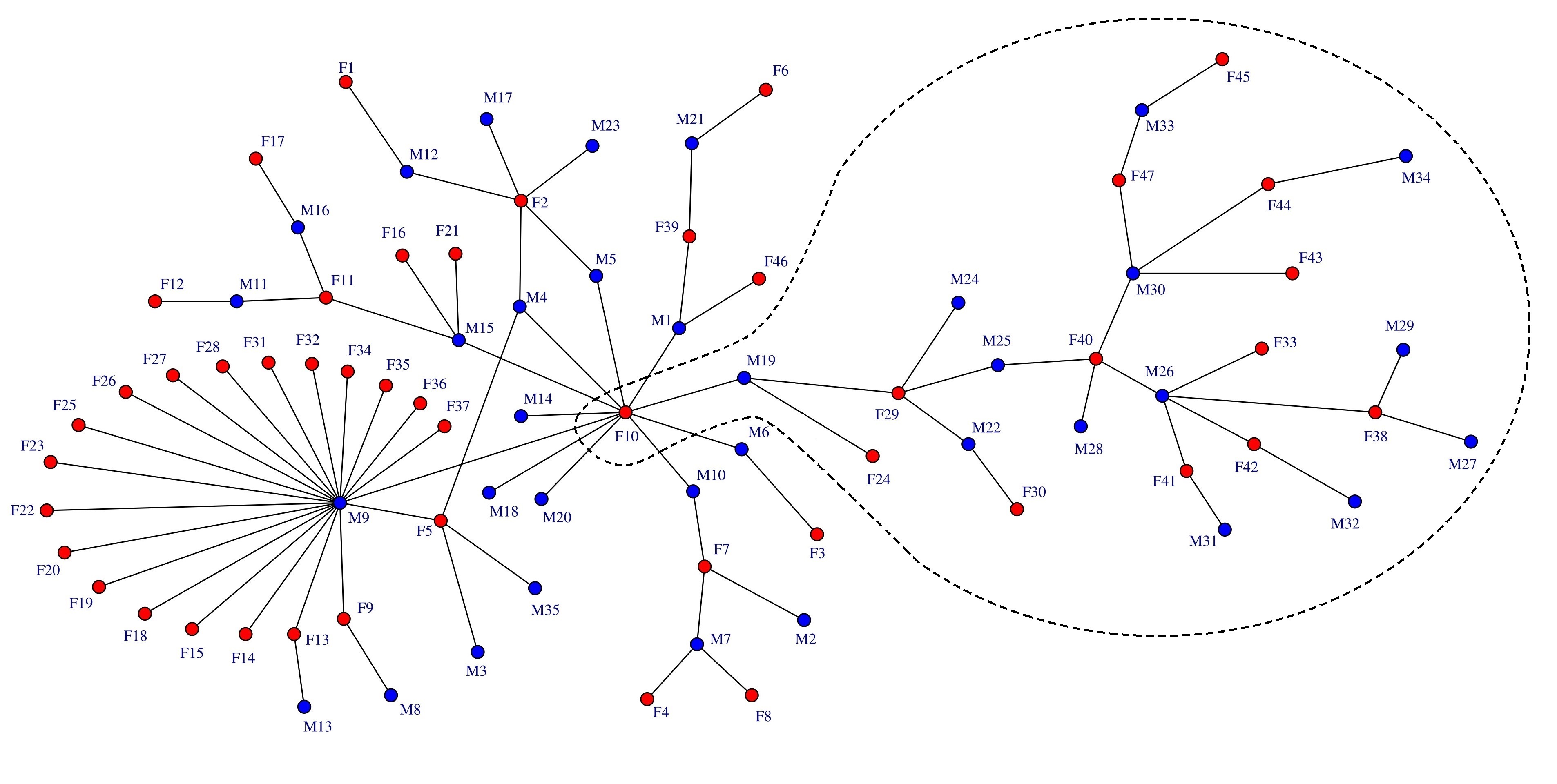
(a)

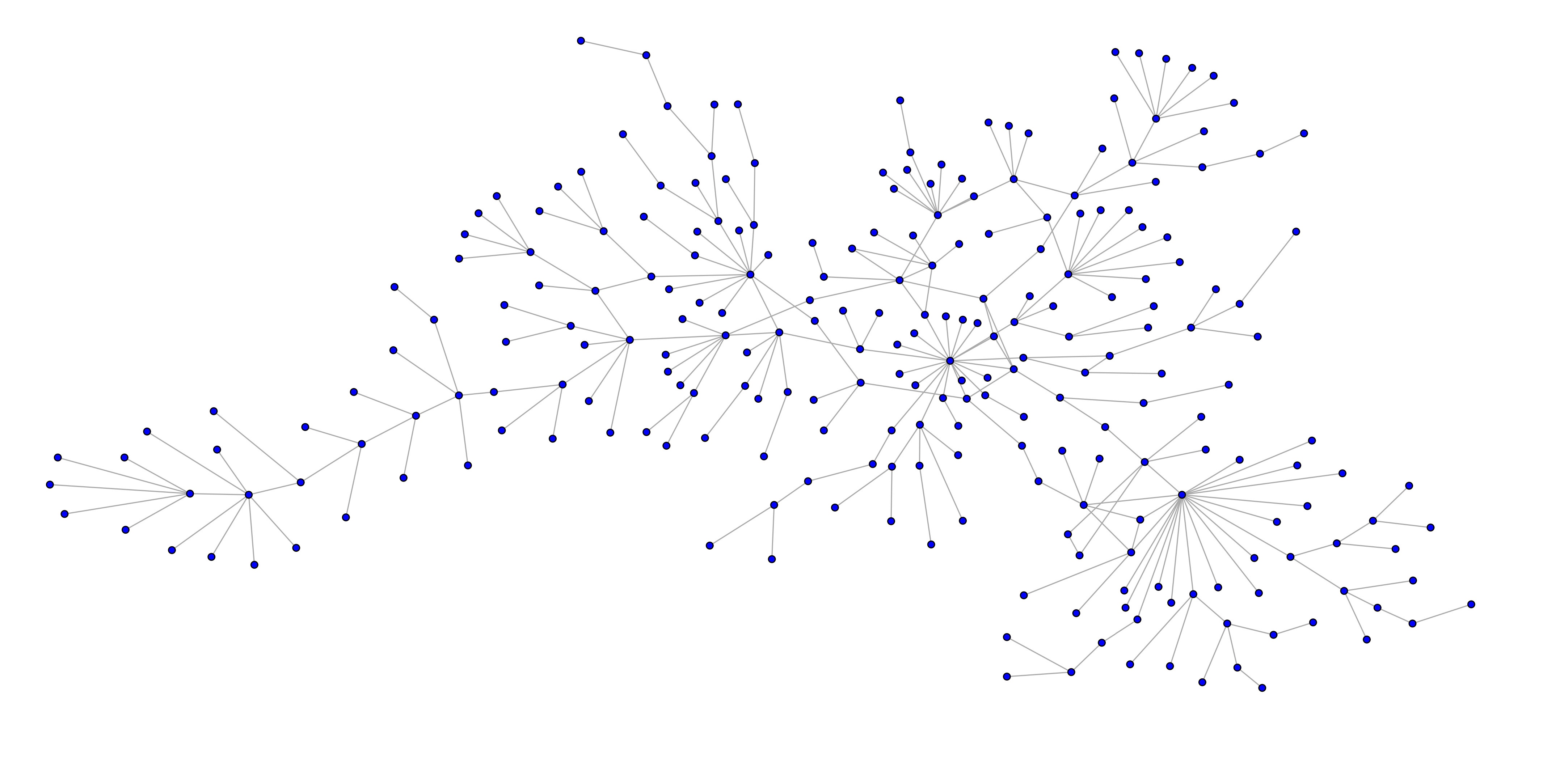
(b)

Figure 2: Illustration of the networks of (a) heterosexual contacts (NHeC) and (b) homosexual contacts (NHoC) studied in the paper. In the NHeC, the nodes are labelled by the sex of the individuals, M for male and F for female. The block of individuals residing in Winnipeg are sketched with a broken line. The rest are from Northern Manitoba.

In Table 1 we compare some of the general parameters of both networks (see [30] for definitions and examples): (i) edge density $\delta=2m/n\left(n-1\right)$ where $m$ is the number of edges, (ii) average shortest path length $\bar{l}$, (iii) average Watts-Strogatz clustering coefficient $\bar{C}$ (see also [31]), (iv) degree heterogeneity $\rho$ (see also [32, 33]), (v) spectral radius of the adjacency matrix $\lambda_{1}$ (see also [34]), and (vi) degree assortativity $r$ (see also [35]). As can be seen, the two networks are very similar to each other, except that the network of heterosexual contacts (NHeC) is bipartite and thus it contains no odd cycles, which implies that the clustering coefficient is zero, while the network of homosexual contacts (NHoC) is not bipartite and it has clustering different from zero. Both networks are poorly dense, although the NHeC is more densely connected than the NHoC. The degree heterogeneity of both networks is relatively small, their spectral radii are very close to each other, and both networks are degree disassortative indicating a preference of high degree nodes of being connected with low degree ones.

property	Heterosexual	Homosexual
$\delta$	0.025	0.0085
$\bar{l}$	5.387	8.327
$\bar{C}$	0	0.0298
$\rho$	0.0154	0.0159
$\lambda_{1}$	4.7333	4.8454
$r$	-0.0458	-0.2782

Table 1: A few topological parameters of the two networks of sexual contacts analyzed: $\delta$ is the edge density; $\bar{l}$ is the average path length; $\bar{C}$ is the average Watts-Strogatz clustering coefficient; $\rho$ is the degree heterogeneity; $\lambda_{1}$ is the spectral radius of the adjacency matrix; $r$ is the degree assortativity.

The main goal of this section is to compare the networked SIS model and the Gompertz-like solution produced as an upper bound of the SIS model. The SIS model is used for sexually transmitted diseases where individuals can get repeatedly infected. Eames and Keeling [36, 37] provide some specific values for $\beta_{e}$ for both Chlamydia and Gonorrhoea, according to the different models used to describe the virus spreading in the same network we analyze here. For the purposes of our numerical analysis it is enough to keep a mean value equal to $\beta_{e}=1.5$. Therefore, we will consider a disease propagating through these two sexual networks, for which we use the following parameters: $\beta=0.03$, $\gamma=0.02$ and $\beta_{e}=1.5$. In both cases we consider the same probability $p,$ which for the NHeC is $1/82$ and for the NHoC is $3/250$. This choice is equivalent to a single initially infected individual in the NHeC; an equal initial probability is then adopted in the NHoC to compare the time evolution of the epidemics in both.

2.3 Time evolution of the cumulative probability

We start our analysis by considering the time evolution of the cumulative number of infected individuals in both networks. In Fig. 3 we illustrate the results of the simulations with the parameters given before using the exact solution of the SIS model (panel (a)) as well as with the Gompertz-like solution of the worst-case scenario (panel (b)). As can be seen in panel (a) the evolution of the infection predicted by the SIS model is practically identical for both networks up to approximately $t=40$. From that time the propagation of the infection in the NHoC is faster than in the NHeC. In the steady state the number of infected individuals in both networks is below 65% with a slightly bigger percentage in the NHoC than in the NHeC. In the case of the Gompertz-like model the growing process occurs identically for both networks for a longer time than in the SIS model, i.e., up to $t=50$ (see panel (b)). Also, after this time the infection grows faster in the NHoC reaching the 100% of infected individuals at $t=90$ while the NHeC reaches the saturation at $t=110$.

To gain more insights about the importance of these differences we consider some data observed empirically in [28]. According to this observation the branch formed by individuals $F6-M21-F39-M1-F46-F10$ (branch 1) turned out to be completely infected while the branch of individuals $F45-M33-F47-M30-F43-F4$0 (branch 2) was not completely infected at the same time (only 66.7% of individuals infected). Notice that both branches contains the same number of nodes, as well as the same proportion of males/females. As can be seen in Fig. 3 (panel (c)) the exact solution of the SIS model predicts a faster growth of the infection in branch 1, but when this branch reaches its maximum, which is not 100% of infected nodes, the difference with branch 2 is insignificant. This indicates that using SIS we cannot observe branch 1 completely infected and branch 2 only partially infected. The Gompertz approach (see panel (d)) also predicts a faster growth of the infection on branch 1, but with bigger differences than in the case reported by SIS. For instance, at $t=80$, SIS predicts 45.7% of infection in branch 1 and 35.4% in branch 2, while Gompertz predicts 90.9% for branch 1 and only 56.1% for branch 2. More importantly, at $t=100$ all the nodes in branch 1 are infected, while the probability of being infected for nodes in branch 2 is below 80%. Therefore, in this case we can reproduce, even without fitting the parameters $\beta$ and $\gamma$, what has been observed empirical in the real-world evolution of a sexually transmitted disease in this network.

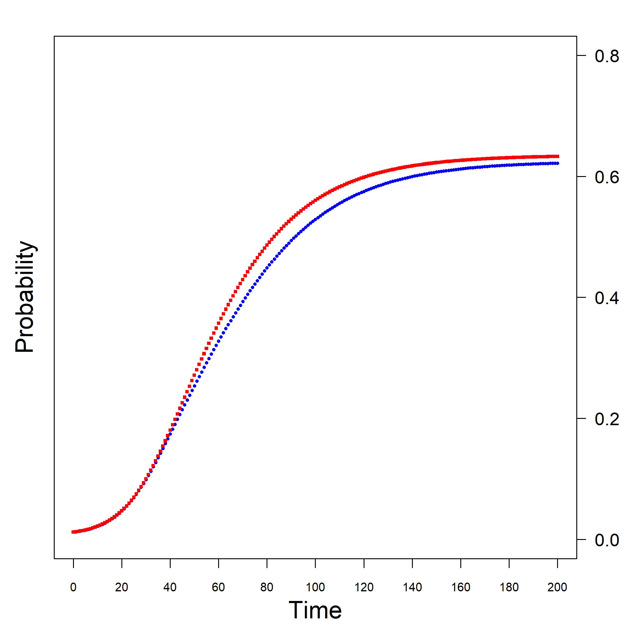
(a)

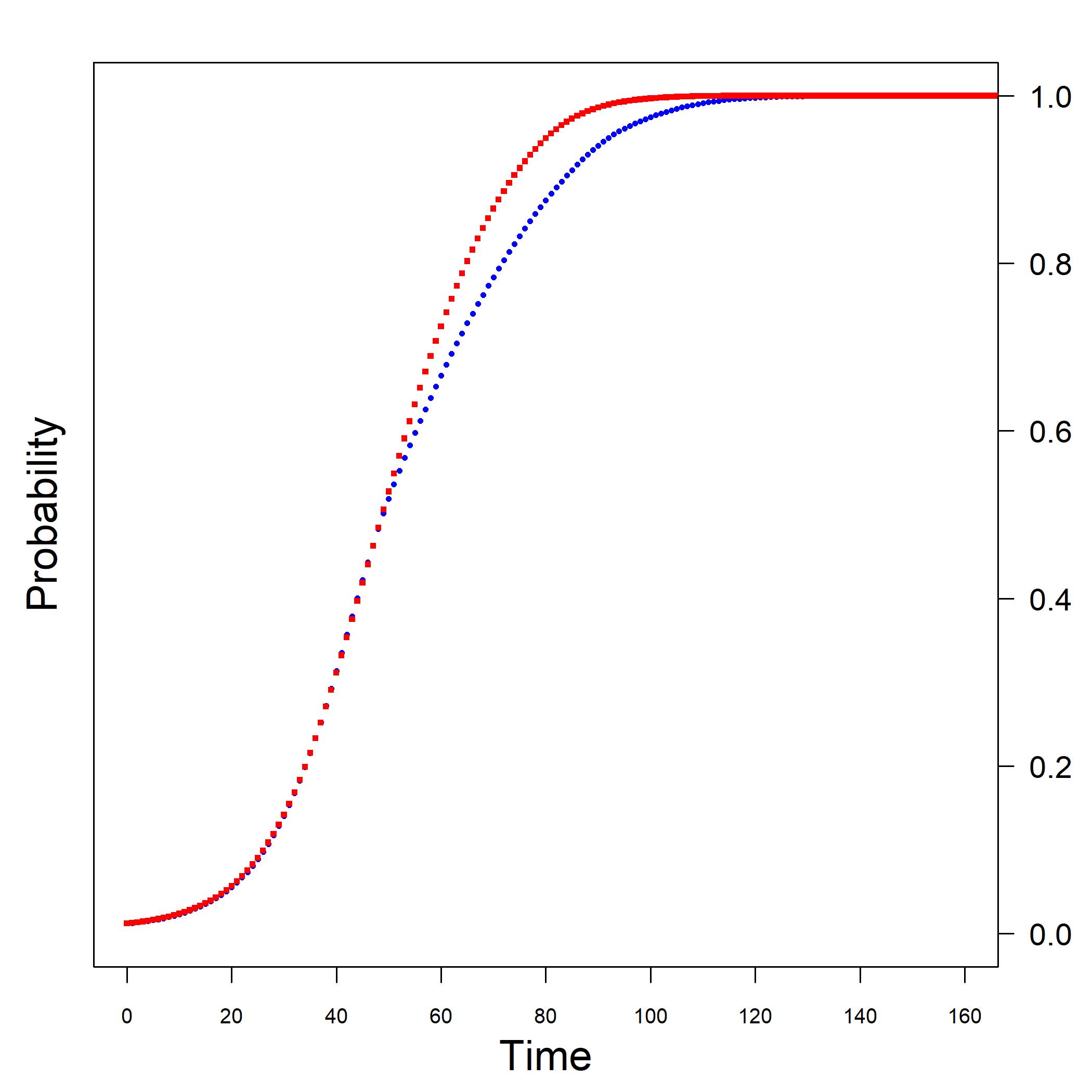
(b)

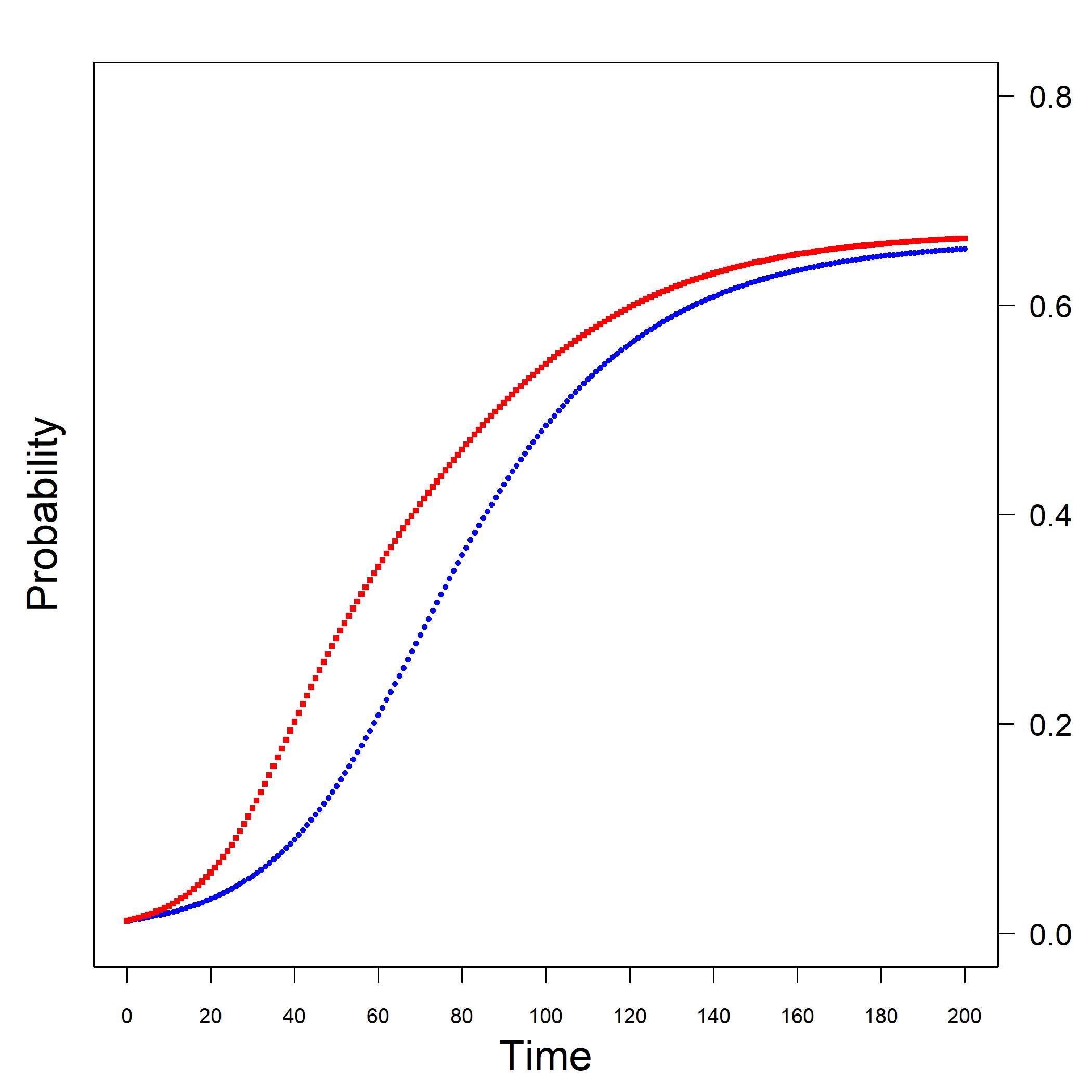
(c)

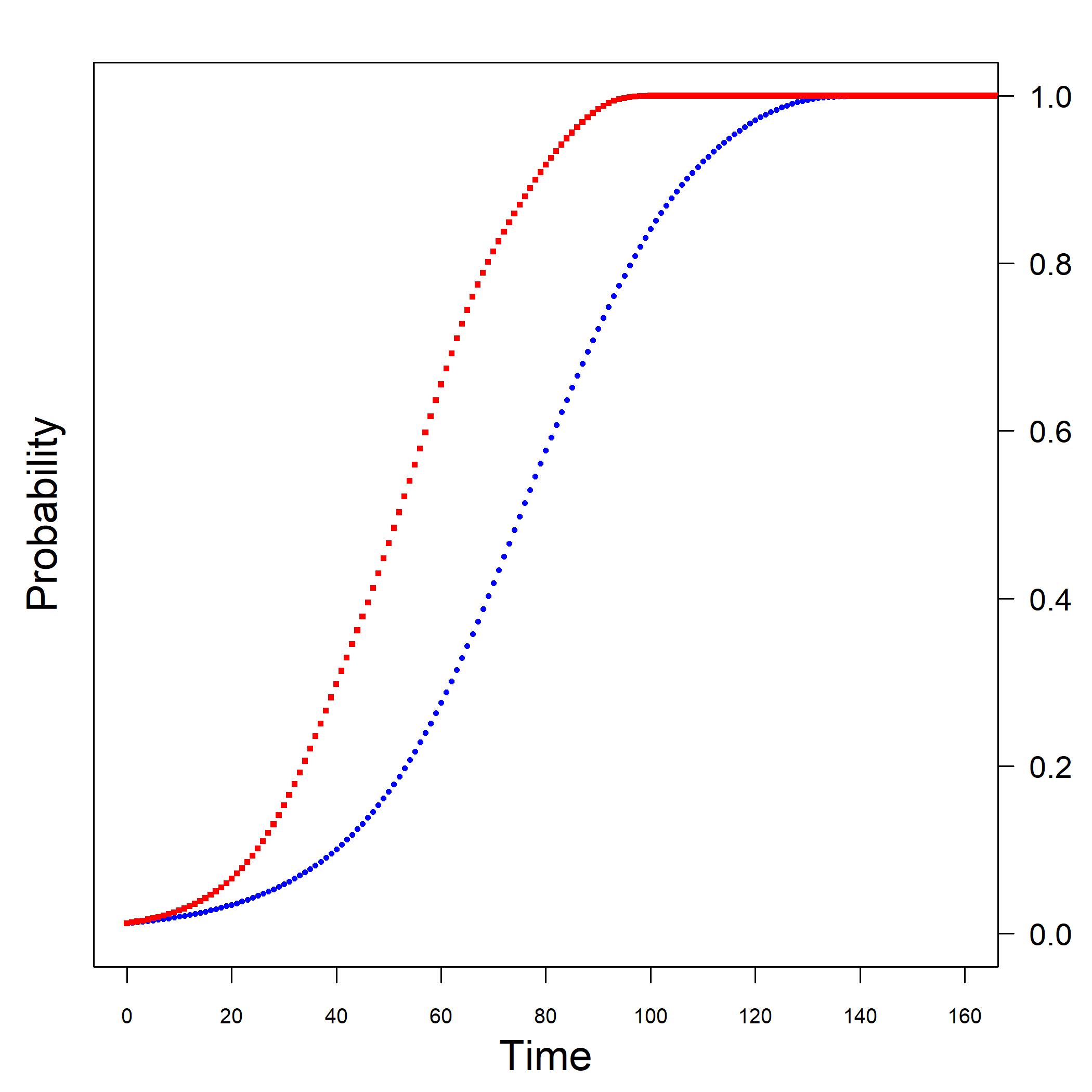
(d)

Figure 3: Illustration of the time evolution of the cumulative probability of getting infected obtained for the networks of hetero- and homosexual contacts using the SIS model (a) and the Gompertz-like solution obtained in this work (b). In panels (a) and (b) red circular dots curve refers to the NHoC and blue square dots curve to the NHeC. The time evolution of the cumulative probability of two branches of the NHeC is obtained with the SIS model (c) and the Gompertz-like solution obtained in this work (d). In panels (c) and (d) red circular dots curve refers to branch 1 and blue square dots curve to branch 2 (see the text for the involved nodes).

2.4 Temporal analysis of the probability density

We now turn our attention to the time evolution of the population density of infected individuals. As can be seen in Fig. 4 (panel (a)), according to SIS, the growing period is practically the same in both networks, with the NHoC reaching a higher peak than the NHeC. Both networks reach their maximum number of infected individuals almost at the same time. The number of infected individuals per unit time decays slightly faster in the NHoC than in the NHeC, and both curves finally reach the zero percent of infected individuals at the same time.

In the case of the Gompertz-like model (panel (b)) the differences are more marked between the time evolution of the infection in both networks. Here again the infection has the same growing process for both networks, but from this time the differences of the dynamics in the two networks are more significant. From $t=40$ to $t=75$ the infection decays faster in the NHeC. From that time on, the decay is faster in the NHoC. Another important characteristic observed in panel (b) is that while the whole decay in the NHoC is smooth, it is irregular for the case of the NHeC.

In order to further investigate the non smooth decay of the probability density of infected individuals in the network of heterogeneous sexual contacts we perform the same analysis by separating the nodes according to the sex of the corresponding individuals. As can be seen in Fig. 4 (panel (c) and (d)) both approaches (SIS and Gompertz, respectively) predict a faster growing process for females than for males, with a more pronounced difference in the Gompertz approach. However, while the SIS approach predicts smooth decays of the number of infected males and females, the Gompertz approach predicts an irregular decay for males with two shoulders at different times, and a clearly non-monotonic decay for females where a second peak is observed at about $t=80$.

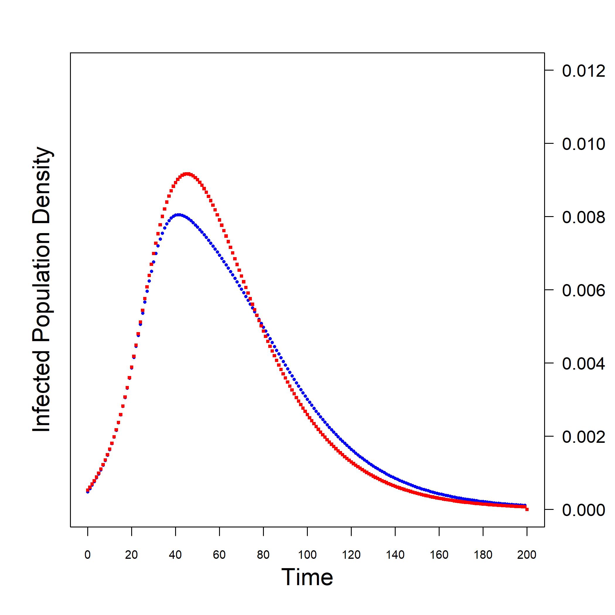
(a)

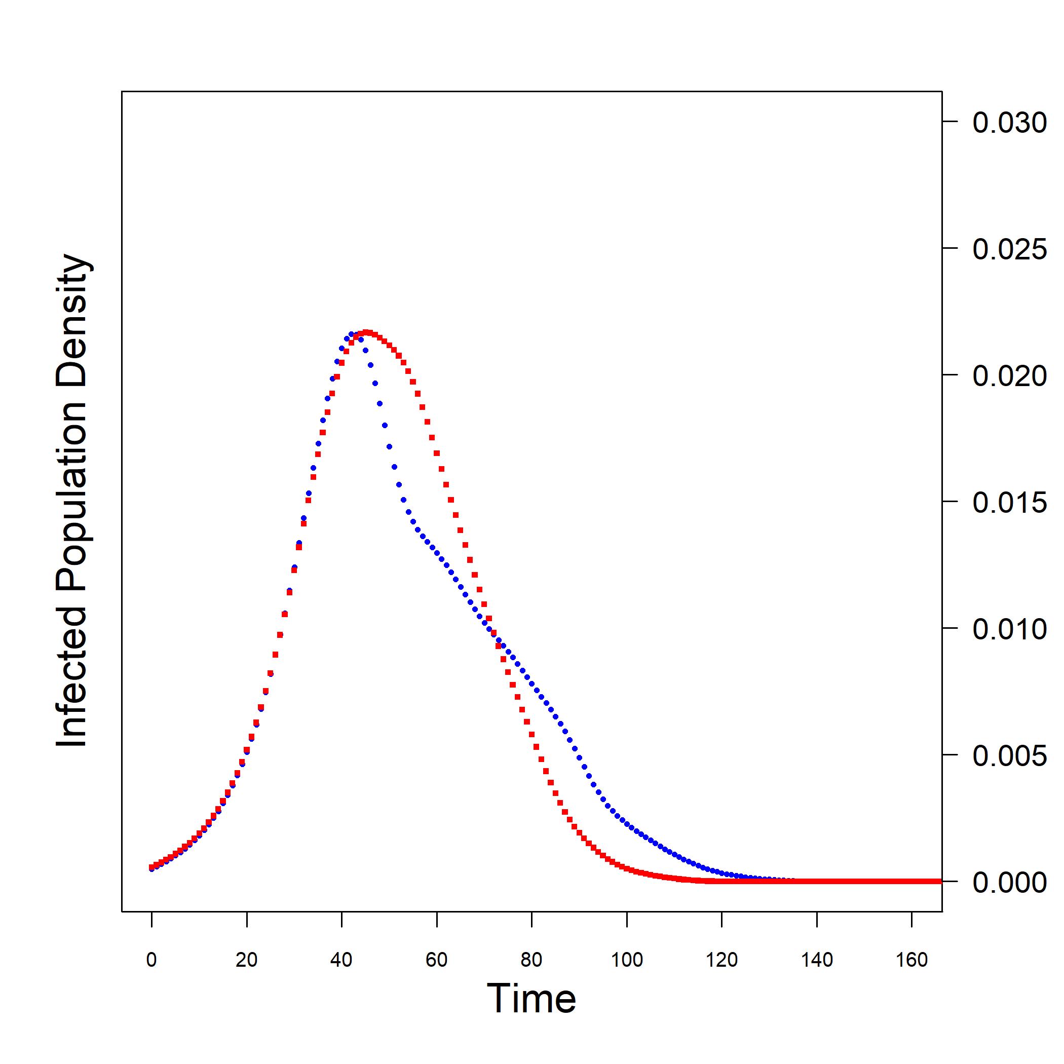
(b)

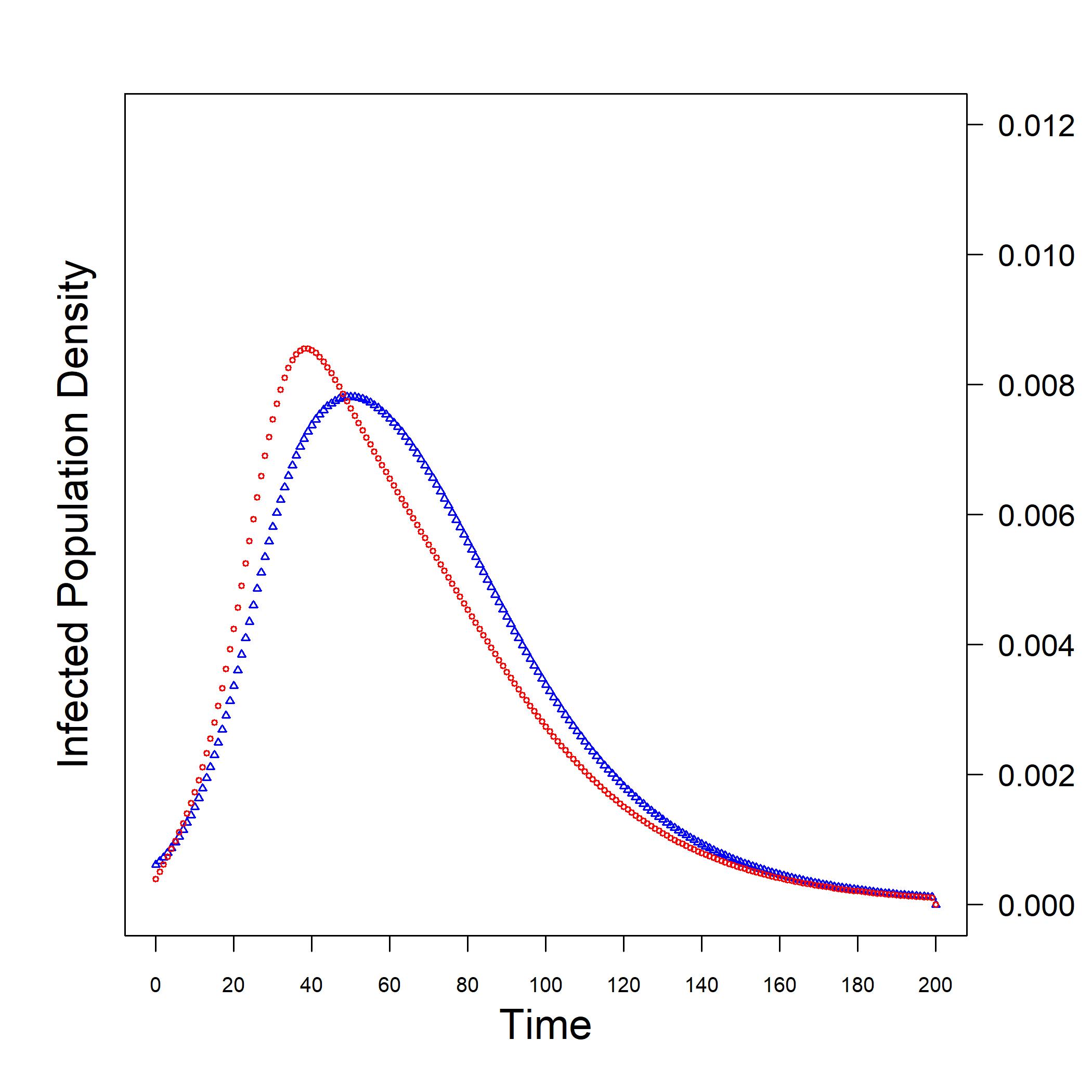
(c)

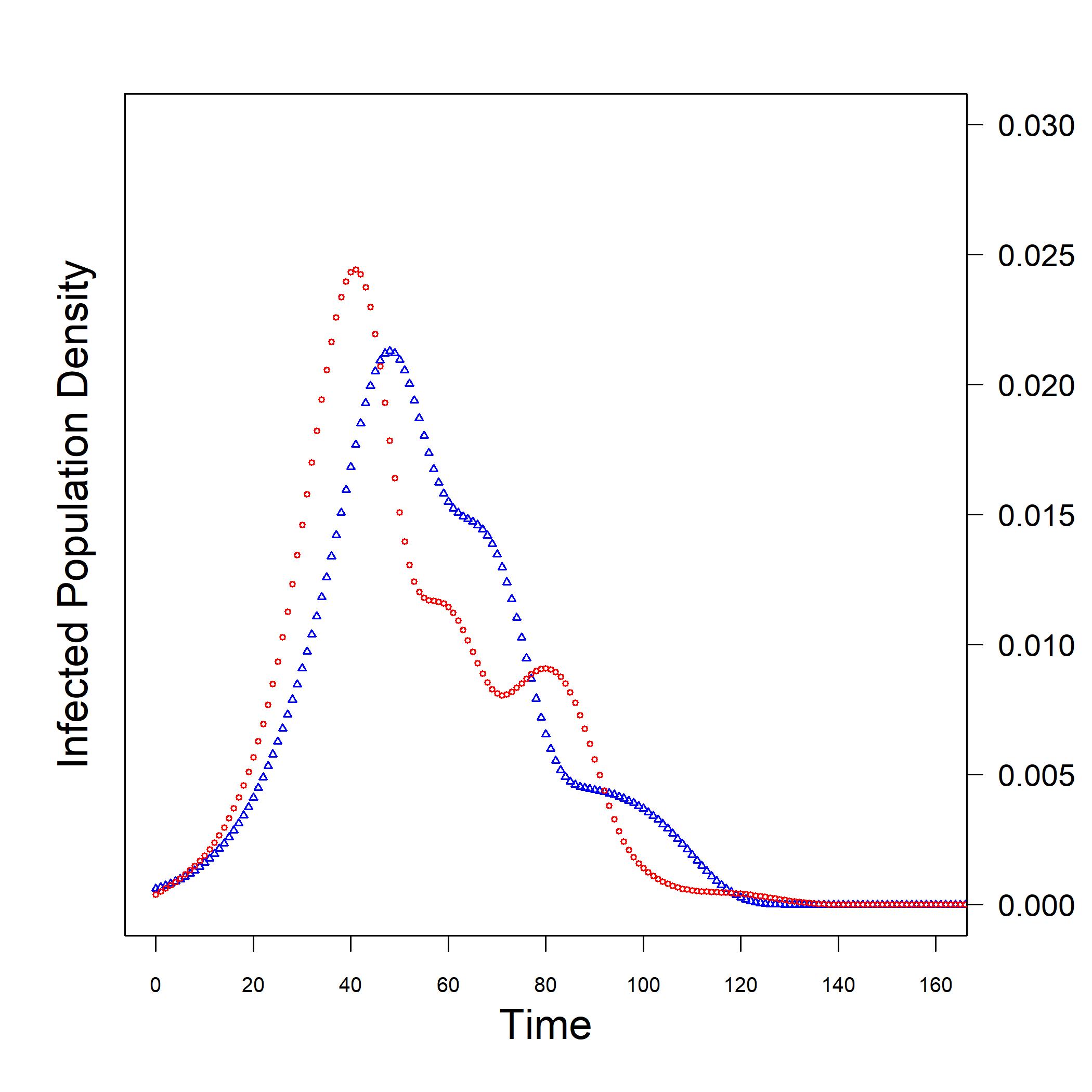
(d)

Figure 4: Illustration of the time evolution of the probability density of getting infected obtained for the networks of hetero- and homosexual contacts using the SIS model (a) and the Gompertz-like solution obtained in this work (b). In panels (a) and (b) red circular dots curve refers to the NHoC and blue square dots curve to the NHeC. The time evolution of the probability density of males and females in the NHeC is obtained with the SIS model (c) and the Gompertz-like solution obtained in this work (d). In panels (c) and (d) red circles curve refers to the female component and blue triangles curve to the male component.

In the literature appear several reasons for this kind of “multiple peaks” behavior in the dynamics of diseases. In the review paper [38] the author asks the question: “What is the mechanism(s) that is generating the multiple peaks? Nobody knows”. In the context of Susceptible-Infected-Recovered (SIR) models the authors of [39] proposed several alternatives, two of which are applicable to the case studied here: (i) changes in pathogen transmissibility and behavioral changes; (ii) population heterogeneity where each wave spreads through one sub-population. In another paper [40] (see also [41]), the authors reported that highly assortative mixing of the contacts tends to lead to more rapid epidemic growth and can produce multiple peaks in disease incidence. An explanation for the influence of assortative mixing and multiple peaks is provided in [42] by considering that the pathogen tends to move gradually from one sexual activity group to the next, where the multiple peaks then correspond to emerging infection within-group epidemics. A similar finding is reported in [43]. On the other hand, in [44] the authors are able to generate multiple peaks of the infection by tuning the parameters of a multi-compartment model.

We investigate here the causes of the multiple peaks observed when using the networked Gompertz model. First we notice that the NHeC consists of two main blocks which corresponds to individuals living in northern Manitoba and in Winnipeg. We then select nodes representing female individuals from both blocks, namely F10, F37, F1 and F4 from the block of Northern Manitoba (left in Fig. 2 (a)) and F43 and F45 from the block of Winnipeg (right in Fig. 2 (a)). In Fig. 5 we illustrate the results of the progression of the infection through these nodes. We have initiated the process by considering that every node has exactly the same probability of getting infected, i.e. $p=1/82$. However, as “all roads lead to Rome”, node M9, which has the highest degree of the network (degree 21), has a high risk of contagion at earlier times of the propagation of the infection. Then, it is very clear in the figure that among the nodes selected here, node F10, which is connected to M9 and also has a high degree (degree 11), is the first to reach the peak of infection. Then, it comes F37, which is a node separated by only three steps from M9. The process continues by infecting nodes F1 and F4, which are five steps away from M9, with the difference that the infection has two routes to infect F1 (there is a square: F10-M4-F2-M5-F10) and only one to infect F4. Then, the infection jumps to the second block and infects node F43 separated from M9 by seven steps and then F45 separated by nine steps from M9.

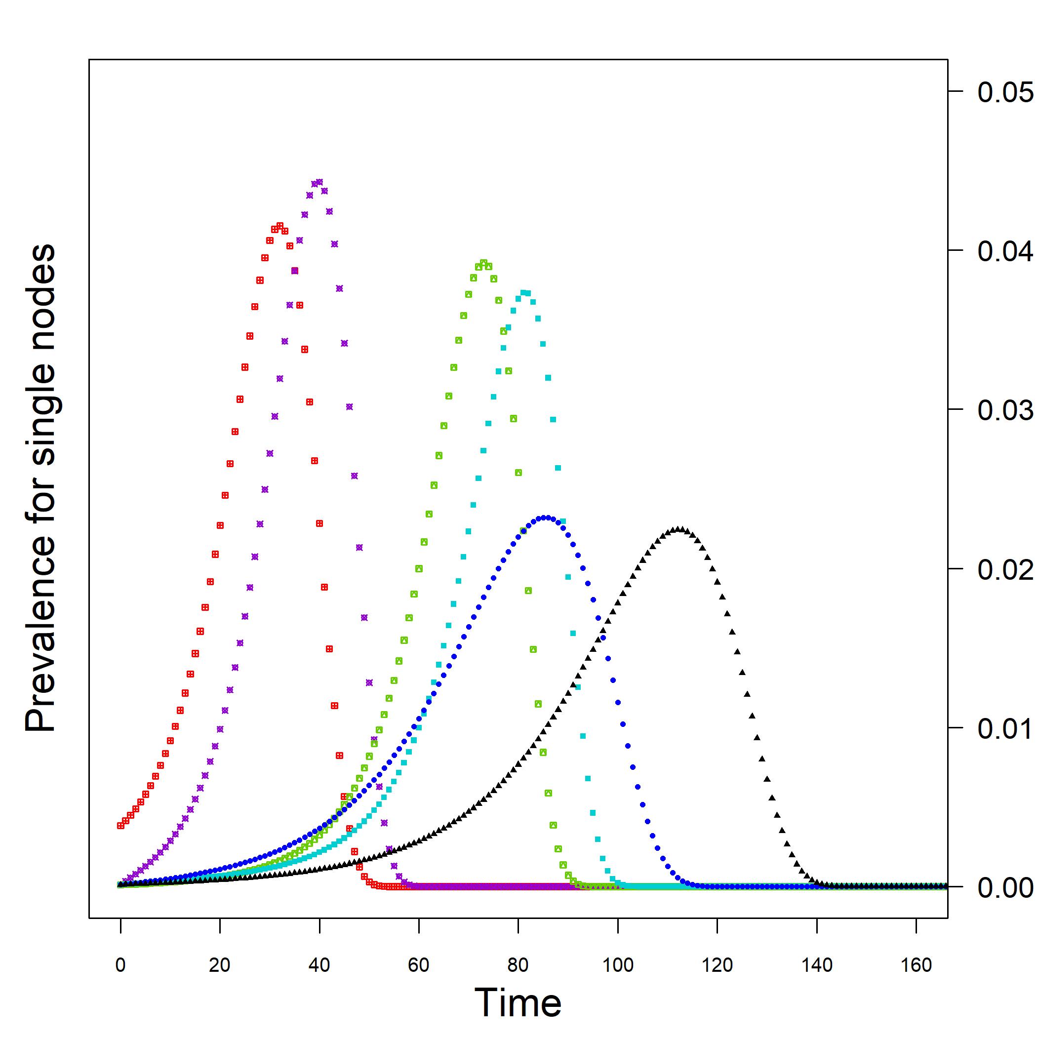
Figure 5: Illustration of the time evolution of the probability density of getting infected obtained for several nodes representing female individuals located at different “regions” of the network of heterosexual contacts (NHeC) using the Gompertz-like solution obtained in this work. From left to right: red F10; violet F37; green F1; cyan F4; blue F43; black F45.

This result indicates that the networked Gompertz model obtained here captures the wavefront nature of the propagation of a disease on a network when more than one block or cluster exist. As we have seen before this important feature of epidemic propagation is not captured by the exact solution of the SIS model. Multipeaks like the ones reproduced by the current model are observed in several real-life epidemics, ranging from the dengue fever outbreak in Havana (see Fig. 6 in [38]) to the swine fever virus outbreaks in the Netherlands during 1997-1998 (see Fig. 7 in [38] and [45]). Additionally, as the NHeC studied here is degree disassortative, our results show that the condition of assortativity is not necessary for the existence of these multipeaks as previously claimed in the literature [40].

3 Conclusions

It is known that the Gompertz function has a remarkable effectiveness in fitting experimental epidemiological and biological data, including the worldwide spread of COVID-19. Here we approach the problem of combining this specific function with the information about the structure of real networks hosting a contagion process. To the best of our knowledge, a Gompertz function on networks has not been proposed in the literature so far. This function should take into account the topological structure of the network and at the same time reduce asymptotically to the scalar Gompertz function for sufficiently large times. The present paper fills this gap, presenting a deduction of a Gompertz function on networks starting from a classical contagion model such as the SIS model, which, as is well known, is characterized by a symmetrical behavior with respect to the inflection point. The search for an upper bound for the exact solution to the SIS model on network has led to the identification of a new class of functions that lack such symmetry but instead exhibit a typical Gompertz behavior. We test this function on networks of sexual contacts that have already been analyzed in the literature as the site of transmission for various infectious diseases, which contemplate the possibility that a recovered individual could become infected again. The main results can be summarized as follows: 1) the function deduced as a worst-case scenario of the SIS model describes effectively the behavior of the exact solution simulated on the network under examination; 2) it allows to grasp the different behavior of separate clusters in the network, such as the two components in a bipartite network or specific subsets of nodes; 3) it allows to amplify and therefore better highlight some behaviors reported in the literature in the number of daily cases, such as the existence of multiple peaks of subsequent infections, or the spread of infection from the core towards the periphery of the network itself. Just as the scalar Gompertz curve finds application in the description of an ever increasing number of growth processes, we are confident that the function proposed here could help in the description of similar processes hosted on specific networks.

References

- [1] B. Gompertz, XXIV. On the nature of the function expressive of the law of human mortality, and on a new mode of determining the value of life contingencies. in a letter to Francis Baily, Esq. F.R.S.&c, Philosophical transactions of the Royal Society of London (115) (1825) 513–583.
- [2] K. Oshima, I. Hofuku, Modified Gompertz curve and its applications I, in: Proceedings of the Sixth International Colloquium on Differential Equations, De Gruyter, 2020, pp. 181–188.
- [3] C. E. Finch, M. C. Pike, Maximum life span predictions from the Gompertz mortality model, The Journals of Gerontology Series A: Biological Sciences and Medical Sciences 51 (3) (1996) B183–B194.
- [4] D. Yang, P. Gao, C. Tian, Y. Sheng, Gompertz tracking of the growth trajectories of the human-liver-cancer xenograft-tumors in nude mice, Computer methods and programs in biomedicine 191 (2020) 105412.
- [5] L. E. B. Cabrales, J. I. Montijano, M. Schonbek, A. R. S. Castañeda, A viscous modified Gompertz model for the analysis of the kinetics of tumors under electrochemical therapy, Mathematics and Computers in Simulation 151 (2018) 96–110.
- [6] A. R. S. Castañeda, E. R. Torres, N. A. V. Goris, M. M. González, J. B. Reyes, V. G. S. González, M. Schonbek, J. I. Montijano, L. E. B. Cabrales, New formulation of the Gompertz equation to describe the kinetics of untreated tumors, PloS one 14 (11) (2019) e0224978.
- [7] C. Frenzen, J. Murray, A cell kinetics justification for Gompertz equation, SIAM Journal on Applied Mathematics 46 (4) (1986) 614–629.
- [8] O. Karin, A. Agrawal, Z. Porat, V. Krizhanovsky, U. Alon, Senescent cell turnover slows with age providing an explanation for the Gompertz law, Nature communications 10 (1) (2019) 1–9.
- [9] R. Gutierrez-Jaimez, P. Román, D. Romero, J. J. Serrano, F. Torres, A new Gompertz-type diffusion process with application to random growth, Mathematical Biosciences 208 (1) (2007) 147–165.
- [10] Y. Li, H. Cheng, J. Wang, Y. Wang, Dynamic analysis of unilateral diffusion Gompertz model with impulsive control strategy, Advances in Difference Equations 2018 (1) (2018) 1–14.
- [11] E. E. Ramirez-Torres, A. R. S. Castaneda, L. Randez, L. E. V. García, L. E. B. Cabrales, S. A. Sisson, J. I. Montijano, A new model of unreported COVID-19 cases outperforms three known epidemic-growth models in describing data from Cuba and Spain, medRxiv.
- [12] R. Conde-Gutiérrez, D. Colorado, S. Hernández-Bautista, Comparison of an artificial neural network and Gompertz model for predicting the dynamics of deaths from COVID-19 in México, Nonlinear Dynamics (2021) 1–15.
- [13] Á. Berihuete, M. Sánchez-Sánchez, A. Suárez-Llorens, A bayesian model of COVID-19 cases based on the Gompertz curve, Mathematics 9 (3) (2021) 228.
- [14] J. A. M. Valle, Predicting the number of total COVID-19 cases and deaths in Brazil by the Gompertz model, Nonlinear Dynamics 102 (4) (2020) 2951–2957.
- [15] A. Ohnishi, Y. Namekawa, T. Fukui, Universality in COVID-19 spread in view of the Gompertz function, Progress of Theoretical and Experimental Physics 2020 (12) (2020) 123J01.
- [16] A. Nobile, L. Ricciardi, L. Sacerdote, On Gompertz growth model and related difference equations, Biological Cybernetics 42 (3) (1982) 221–229.
- [17] T. Grozdanovski, J. Shepherd, Slow variation in the Gompertz model, ANZIAM Journal 47 (2005) C541–C554.
- [18] R. Berger, Comparison of the Gompertz and logistic equations to describe plant disease progress., Phytopathology 71 (7) (1981) 716–719.
- [19] M. Dhar, P. Bhattacharya, Comparison of the logistic and the Gompertz curve under different constraints, Journal of Statistics and Management Systems 21 (7) (2018) 1189–1210.
- [20] M. A. Achterberg, B. Prasse, L. Ma, S. Trajanovski, M. Kitsak, P. Van Mieghem, Comparing the accuracy of several network-based COVID-19 prediction algorithms, International journal of forecasting.
-
[21]
H.-J. Li, W. Xu, S. Song, W.-X. Wang, M. Perc,
The
dynamics of epidemic spreading on signed networks, Chaos, Solitons &
Fractals 151 (2021) 111294.
doi:https://doi.org/10.1016/j.chaos.2021.111294.
URL https://www.sciencedirect.com/science/article/pii/S0960077921006482 - [22] C.-H. Lee, S. Tenneti, D. Y. Eun, Transient dynamics of epidemic spreading and its mitigation on large networks (2019). arXiv:1903.00167.
- [23] C.-H. Lee, S. Tenneti, D. Y. Eun, Transient dynamics of epidemic spreading and its mitigation on large networks, in: Proceedings of the twentieth ACM international symposium on mobile ad hoc networking and computing, 2019, pp. 191–200.
- [24] L. Katz, A new status index derived from sociometric analysis, Psychometrika 18 (1) (1953) 39–43.
- [25] E. Estrada, D. J. Higham, Network properties revealed through matrix functions, SIAM Rev. 52 (4) (2010) 696–714.
- [26] D. Juher, J. Saldaña, R. Kohn, K. Bernstein, C. Scoglio, Network-centric interventions to contain the syphilis epidemic in San Francisco, Scientific reports 7. doi:10.1038/s41598-017-06619-9.
- [27] S. Zhao, S. S. Musa, H. Fu, D. He, J. Qin, Simple framework for real-time forecast in a data-limited situation: the Zika virus (ZIKV) outbreaks in Brazil from 2015 to 2016 as an example, Parasites & Vectors 12 (1) (2019) 344–357. doi:10.1186/s13071-019-3602-9.
- [28] J. L. Wylie, A. Jolly, Patterns of chlamydia and gonorrhea infection in sexual networks in Manitoba, Canada, Sexually transmitted diseases 28 (1) (2001) 14–24.
- [29] J. J. Potterat, L. Phillips-Plummer, S. Q. Muth, R. Rothenberg, D. Woodhouse, T. Maldonado-Long, H. Zimmerman, J. Muth, Risk network structure in the early epidemic phase of HIV transmission in Colorado Springs, Sexually transmitted infections 78 (suppl 1) (2002) i159–i163.
- [30] E. Estrada, The structure of complex networks: theory and applications, Oxford University Press, 2012.
- [31] D. J. Watts, S. H. Strogatz, Collective dynamics of ’small-world’ networks, nature 393 (6684) (1998) 440–442.
- [32] E. Estrada, Quantifying network heterogeneity, Physical Review E 82 (6) (2010) 066102.
- [33] E. Estrada, Degree heterogeneity of graphs and networks. I. Interpretation and the "heterogeneity paradox", Journal of Interdisciplinary Mathematics 22 (4) (2019) 503–529.
- [34] D. Stevanovic, Spectral radius of graphs, Academic Press, 2014.
- [35] M. E. Newman, Mixing patterns in networks, Physical review E 67 (2) (2003) 026126.
- [36] K. T. D. Eames, M. J. Keeling, Modeling dynamic and network heterogeneities in the spread of sexually transmitted diseases, Proceedings of the National Academy of Sciences 99 (20) (2002) 13330–13335. doi:10.1073/pnas.202244299.
- [37] M. J. Keeling, K. T. Eames, Networks and epidemic models, Journal of the Royal Society Interface 2 (4) (2005) 295–307.
- [38] H. H. Weiss, The SIR model and the foundations of public health, Materials matematics (2013) 0001–17.
- [39] A. Mummert, H. Weiss, L.-P. Long, J. M. Amigó, X.-F. Wan, A perspective on multiple waves of influenza pandemics, PloS one 8 (4) (2013) e60343.
- [40] S. Gupta, R. M. Anderson, R. M. May, Networks of sexual contacts: implications for the pattern of spread of HIV, AIDS (London, England) 3 (12) (1989) 807–817.
- [41] R. M. Anderson, Discussion: the Kermack-McKendrick epidemic threshold theorem, Bulletin of mathematical biology 53 (1) (1991) 1–32.
- [42] S. Hertog, Heterosexual behavior patterns and the spread of HIV/AIDS: the interacting effects of rate of partner change and sexual mixing, Sexually transmitted diseases 34 (10) (2007) 820–828.
- [43] Z. Xu, Z. Zu, T. Zheng, W. Zhang, Q. Xu, J. Liu, Long-distance travel behaviours accelerate and aggravate the large-scale spatial spreading of infectious diseases, Computational and mathematical methods in medicine 2014.
- [44] N. Perra, D. Balcan, B. Gonçalves, A. Vespignani, Towards a characterization of behavior-disease models, PloS one 6 (8) (2011) e23084.
- [45] A. Stegeman, A. Elbers, J. Smak, M. de Jong, Quantification of the transmission of classical swine fever virus between herds during the 1997-1998 epidemic in The Netherlands, Preventive veterinary medicine 42 (3-4) (1999) 219–234. doi:10.1016/s0167-5877(99)00077-x.