From Tree Tensor Network to Multiscale Entanglement Renormalization Ansatz

Abstract

Tensor Network States (TNS) offer an efficient representation for the ground state of quantum many body systems and play an important role in the simulations of them. Numerous TNS are proposed in the past few decades. However, due to the high cost of TNS for two-dimensional systems, a balance between the encoded entanglement and computational complexity of TNS is yet to be reached. In this work we introduce a new Tree Tensor Network (TTN) based TNS dubbed as Fully-Augmented Tree Tensor Network (FATTN) by releasing the constraint in Augmented Tree Tensor Network (ATTN). When disentanglers are augmented in the physical layer of TTN, FATTN can provide more entanglement than TTN and ATTN. At the same time, FATTN maintains the scaling of computational cost with bond dimension in TTN and ATTN. Benchmark results on the ground state energy for the transverse Ising model are provided to demonstrate the improvement of accuracy of FATTN over TTN and ATTN. Moreover, FATTN is quite flexible which can be constructed as an interpolation between Tree Tensor Network and Multiscale Entanglement Renormalization Ansatz (MERA) to reach a balance between the encoded entanglement and the computational cost.

I Introduction

Understanding exotic phases and exotic phase transitions in strongly correlated quantum many body systems is one of the most challenging topics in condensed matter physics Cabra et al. (2012); Gang (2007); Marino (2017). Due to the lack of analytic solutions, most studies of these systems depend on many-body numerical approaches LeBlanc et al. (2015). For quantum many body systems, the exponential increase of the dimension of the Hilbert space prevents us from studying system with large sizes. Quantum Monte Carlo is an efficient method for quantum many body systems, but it usually suffers from the infamous minus sign problem for Fermionic systems Loh et al. (1990); Troyer and Wiese (2005). For a local Hamiltonian, the ground state and low energy excited states satisfy the well-known entanglement-entropic area law Plenio et al. (2005); Vidal et al. (2003); Srednicki (1993); Eisert et al. (2010), asserting that if we divide the studied system into two parts, the entanglement entropy is proportional to the measure of the partition’s boundary rather than its volume. Hence, if we are only interested in the low-lying states, we only need to consider states which satisfy the entanglement-entropic area law in the Hilbert space. Tensor Network States (TNS) Silvi et al. (2019); Orús (2014); Bridgeman and Chubb (2017) can efficiently encode the entanglement-entropic area law by design, which can faithfully represent the ground state of quantum many body systems. In recent years, significant advances in TNS have been made and they are becoming one of the most popular approaches in studying strongly correlated quantum many body systems Zheng et al. (2017); Liao et al. (2017). During the last three decades, after realizing the underlying wave-functions in Density Matrix Renormalization Group (DMRG) White (1993, 1992); Fannes et al. (1992); Stoudenmire and White (2012); Schollwöck (2005) are actually Matrix Product States (MPS) Östlund and Rommer (1995); Schollwöck (2011), several types of TNS for higher dimensional systems are proposed, including Tree Tensor Network (TTN) Tagliacozzo et al. (2009); Shi et al. (2006); Silvi et al. (2010); Gerster et al. (2014), Projected Entanglement Pair States (PEPS) Cirac et al. (2021); Vanderstraeten et al. (2021); Verstraete and Cirac (2004a, b); Verstraete et al. (2006) and their generalization Xie et al. (2014), and Multiscale Entanglement Renormalization Ansatz (MERA) Vidal (2008); Evenbly and Vidal (2009a); Vidal (2007); Evenbly and Vidal (2009b).

For (quasi) one dimensional systems, DMRG or MPS based approaches Schollwöck (2011); Fannes et al. (1992) are now the workhorse as it can capture the one dimensional entanglement-entropic area law (with a logarithmic correction for critical systems) with a relatively low computational complexity. However, to study two-dimensional systems with DMRG, the bond-dimension needs to be increased exponentially with the width of the system to be able to capture the entanglement-entropic area law, which makes the study of wide system difficult with DMRG Liang and Pang (1994). PEPS is a straightforward generalization of MPS to two dimension. It can capture the area-law of entanglement entropy for two-dimensional systems by design. However, it suffers from a high computational complexity which is usually higher than $O(D^{10})$ Jiang et al. (2008); Kalis et al. (2012), with $D$ the bond-dimension of PEPS. Moreover, the overlap of PEPSs can’t be calculated exactly Schuch et al. (2007), even though there exist many approaches to calculate it approximately Nishino and Okunishi (1996); Xie et al. (2012); Orús (2014); Vanderstraeten et al. (2021). On the contrary, MERA which is constructed by unitary tensors foo (a), can be contracted exactly but suffers from a much higher computational complexity for two dimensional systems $O(D^{16})$ Evenbly and Vidal (2009a). TTN has a similar structure to MERA. It has a lower computational complexity for two dimensional systems (O$(D^{4})$), but encounters the same problems as the DMRG in 2D because TTN doesn’t encode the two-dimensional entanglement-entropic area law by design. So it is desirable to develop new tensor networks with affordable computational complexity which can also encode high entanglement.

Recently, a new tensor network structure based on TTN: Augmented Tree Tensor Network (ATTN) was proposed in Felser et al. (2021). By placing disentanglers at the physical layer of a TTN, it was claimed that ATTN can capture the entanglement-entropic area-law and at the same time keep a computational complexity of $O(D^{4}d^{2})$, with $d$ the dimension of the physical degree of freedom.

We propose a new structure which can provide larger entanglement but maintain the low computational complexity in this work. In ATTN, no two disentanglers share the same Hamiltonian term. But we find this is not a necessary constraint to maintain a low computational cost. We can augment TTN with disentanglers in a way that no two disentanglers share the same physical index. With this strategy, we generate a Fully-Augmented Tree Tensor Network (FATTN) which can capture the entanglement-entropic area law of $L\log(d^{2})$ (for most cuts on a finite lattice) with a large bond dimension $D$ foo (b) for two-dimensional quantum many body systems on a finite lattice and keep a relatively low computational complexity of $O(D^{4}d^{4})$. So the entanglement captured in FATTN is at least as large as that in a PEPS with bond-dimension $D=d^{2}$. But as we will discuss late, while iPEPS can directly deal with system in the thermodynamic limit, FATTN is suitable for finite lattice with periodic boundary conditions. The optimization and contraction of FATTN is easier than PEPS. In our benchmark calculation of a $8\times 8$ transverse Ising model near the critical point, FATTN gives a relative error of ground state energy of the order of $10^{-5}$ even for $D=50$ which largely improve the accuracy over TTN Tagliacozzo et al. (2009) and ATTN Felser et al. (2021).

The rest of the paper is organized as follows: In Sec. II and Sec. III, we briefly review the TTN and ATTN. We then introduce FATTN and discuss the optimization of it in Sec. IV. Benchmark results are provided in Sec. V. In Sec. VI, we discuss different strategies to place disentanglers in FATTN. We summarize this work in Sec. VII.

II Tree Tensor Network

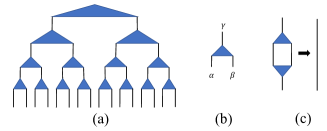
Figure 1: The structure of TTN. In (a), we show an illustration of one dimensional TTN. The building block of TTN: the isometry is shown in (b). In (c), we show that the contraction of an isometry and its conjugate gives an identity tensor from its definition in Eq. (1).

TTN is constructed by placing tensors on a tree structure Silvi et al. (2019). Because it is loop-free, TTN can be efficiently contracted with a computational complexity of $O(D^{4})$. However, at the worst case, it can only provide log$(D)$ entanglement entropy similar as DMRG which means TTN can’t efficiently capture the entanglement-entropic area law of high dimensional systems. To be self-contained, we will give a brief description on the optimization and contraction of TTN following Tagliacozzo et al. (2009), which are the basic steps in approximating the ground state of quantum many systems with TTN.

As shown in Fig. 1, in TTN, a quantum state $|\psi\rangle$ is represented as a contraction of a set of isometries $w_{i}$ foo (c) which are rank-3 tensors with bond-dimension $D$. (For simplicity, we assume that all the bond-dimensions in TTN are the same). The definition of isometry is

$$\sum_{\beta_{1}\beta_{2}}(w_{\beta_{1}\beta_{2}}^{\alpha})(w_{\beta_{1}\beta_{2}}^{\alpha})^{*}=\delta_{\alpha,\alpha^{*}}$$ (1)

(The root tensor is actually a rank-2 tensor, but we can treat it as a rank-3 tensor with the dimension of the third index $1$.) The relationship in Eq. (1) is very useful as they can significantly reduce the computational cost when we perform tensor-tensor contraction in the optimization of TTN and the calculation of physical observables.

In this work, we employ a standard optimization algorithm described in Ref. Evenbly and Vidal (2009b); Tagliacozzo et al. (2009) (For other optimization strategies, we refer the reader to Ref. Evenbly and Vidal (2009b); Haghshenas (2021)). To approximate the ground state of a given Hamiltonian $H$ with a TTN state $|\psi_{\{w\}}\rangle$, we need to find the local tensors of TTN with which the expectation value of the Hamiltonian $E(\{w\})=\langle\psi_{\{w\}}|H|\psi_{\{w\}}\rangle$ is minimized.

Unfortunately, there doesn’t exist an exact solution for this optimization. In practical simulation, we can replace the optimization equation with:

$$E(w_{i})={\rm min}_{w_{i}}\langle\psi_{\{w\}}|H|\psi_{\{w\}}\rangle$$ (2)

where we fix all the isometries except $w_{i}$. With this approximation, the optimization of $w_{i}$ in Eq. (2) is easier. We can optimize $w_{i}$ one by one. The whole procedure can be described as follows. Firstly, we generate a set of initially isometries $(w_{1},w_{2},\dots,w_{n})$ randomly. Then we optimize one of them ($w_{1}$, for example) and fix the others according to Eq. (2). Once $w_{1}$ is optimized, we move to another isometry $w_{2}$ and optimize it in the same way. We iteratively perform this procedure until all the isometries are optimized. This procedure defines one sweep. Then we carry out the next sweeps until the energy is converged according to certain criteria.

So the optimization of the TTN is reduced to minimize the energy in Eq. (2). However, we can not solve this problem exactly either. We follow the approach in Tagliacozzo et al. (2009) where $w_{i}$ and $w_{i}^{*}$ are set to be independent and the optimization problem in Eq. (2) is reduced to

$$E(w_{i})={\rm min}_{w_{i}}\langle\psi_{\{w\}}|H|\psi_{\{w\}}\rangle={\rm min}_{w_{i}}{\rm Tr}(\mathnormal{Y}w_{i})$$ (3)

where we denote the environment of $w_{i}$ in $E(w_{i})$ as $\mathnormal{Y}$. The optimization problem in Eq. (3) can be solved exactly. With a singular value decomposition of the environment $\mathnormal{Y}$:

$$\mathnormal{Y}=USV^{\dagger}$$ (4)

the solution of Eq. (3) can be obtained as $w_{i}=VU^{\dagger}$. We can easily see that this step has a cost of $O(D^{4})$. Fig. 2 shows the procedures of optimizing isometries.

In the following we will show that we can compute the environment $\mathnormal{Y}$ of $w_{i}$ at a cost of $O(D^{4})$. For a given local Hamiltonian, we can decompose it into a sum of a series of two-body operators. So Eq. (3) can be written as:

$$E(w_{i})={\rm min}_{w_{i}}\langle\psi|H|\psi\rangle={\rm min}_{w_{i}}\sum_{j,k}\langle\psi|H_{j,k}|\psi\rangle$$ (5)

where $j,k$ denote the position of the two-body operator.

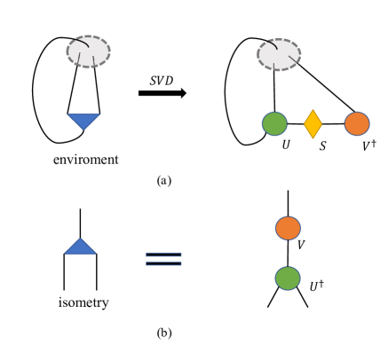
Figure 2: The optimization of the isometry. After the environment tensor $\mathnormal{Y}$ is obtained, a SVD decomposition of it is performed $\mathnormal{Y}=USV^{\dagger}$. The optimized $w_{i}$ is set as $w_{i}=-VU^{\dagger}$. This step also takes a computational cost of $O(D^{4})$.

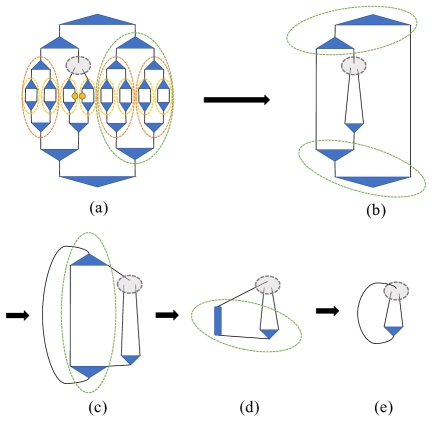
Figure 3: The calculation of the environment for an isometry. We can see that every step has a computational cost of $O(D^{4})$. And the contractions which are not connected with the Hamiltonian term (denoted as the yellow circles) are just identities because of Eq. (1).

Therefore, without loss of generality, we only need to deal with two-site operator (one site term is easy to handle as discussed below). We can further decompose the two-site operator into a sum of direct product of two one-site operators whose number is $d^{2}$ in the worst case with $d$ the dimension of the physical degree of freedom at the physical layer of TTN. Once we compute the contributions from all the terms in the Hamiltonian, we simply add those contributions to get the environment $\mathnormal{Y}$. As shown in Fig. 3, the calculation of the environment $\mathnormal{Y}$ of $w_{i}$ for a two-site operator has a cost of $O(D^{4})$. We can take advantage of Eq. (1) to simplify the calculation as the contraction of two conjugated isometries results in an identity tensor if there is no operator acting on them. As the singular value decomposition of $\mathnormal{Y}$ has a cost of $O(D^{4})$, the overall cost to optimize a TTN is $O(D^{4})$. It is easily to show that the calculation of physical observables also have a cost of $O(D^{4})$. So it is efficient to approximate the ground state of a local quantum Hamiltonian with a TTN. But as mentioned earlier, TTN can’t capture the entanglement-entropic area law for systems in spatial dimension larger than two which hamper its application in simulating two-dimensional many-body systems.

III Augmented Tree Tensor Network

ATTN Felser et al. (2021) was proposed to provide more entanglement entropy than TTN. By placing disentanglers which are unitary tensors satisfying the following condition:

$$\sum_{\beta_{1}\beta_{2}}(u_{\beta_{1}\beta_{2}}^{\alpha_{1}\alpha_{2}})(u_{\beta_{1}\beta_{2}}^{\alpha_{1}\alpha_{2}})^{*}=\delta_{{\alpha_{1}\alpha_{2}},({\alpha_{1}\alpha_{2}})^{*}}$$ (6)

at the physical layer of TTN, the entanglement entropy encode in ATTN scales as $L\log(d)$ Felser et al. (2021). In ATTN, no couple of disentanglers are directly connected by an interaction term in the Hamiltonian to keep a low computational cost. ATTN has a computational complexity of $O(D^{4}d^{2})$ which has the same scaling of $D$ as the TTN. However, a large improvement in numerical precision of ATTN over TTN was shown in Felser et al. (2021).

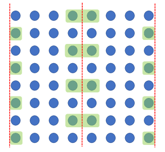
Figure 4: The strategy to place disentanglers in ATTN. Periodic boundary conditions are applied. Blue dots represent the physical layer of 2D TTN and green rectangles are disentanglers. In order to maintain the same $O(D^{4})$ scaling of computational cost as in TTN, no couple of disentanglers are directly connected by a Hamiltonian term. As will be discussed late in the main text, this is not a necessary constraint to keep the $O(D^{4})$ cost.

In Fig. 4 we show the strategies of placing the disentanglers in ATTN for a $8\times 8$ lattice. We can see that a relatively small number of disentanglers are placed to encode the entanglement-entropic area law under the condition that no couple of disentanglers share the same Hamiltonian term.

IV Fully-Augmented Tree Tensor Network

In this section, we propose another TTN based tensor network states which can provide more entanglement over ATTN and at the same time maintain the $O(D^{4})$ computational cost.

IV.1 Position for disentanglers

In ATTN, to maintain a computational complexity compatible with TTN, there are restrictions on how to place disentanglers at the physical layer. We find that the restriction that no couple of disentanglers share the same Hamiltonian term is not necessary to maintain a low computational cost.

We propose a new TTN based tensor network dubbed as Fully Augmented Tree Tensor Network (FATTN). In FATTN, we place disentanglers in a way that no couple of disentanglers share the same physical index. As we will discuss later, the computational cost in FATTN is $O(D^{4}d^{4})$ with $D(d)$ the dimension of bond (physical) indexes. So for an $L\times L$ lattice, we can add $L^{2}/2$ disentanglers at the physical layer. We notice that if more disentanglers are added to the physical layer the TTN becomes a PEPS like structure and exact contraction of them is infeasible in the calculation of physical observables. In Fig. 5, we show an example on how to place disentanglers on a $8\times 8$ lattice in FATTN. Given this constraint, we need to find a strategy to generate the maximum entanglement entropy using these $8^{2}/2$ disentanglers for the $8\times 8$ lattice.

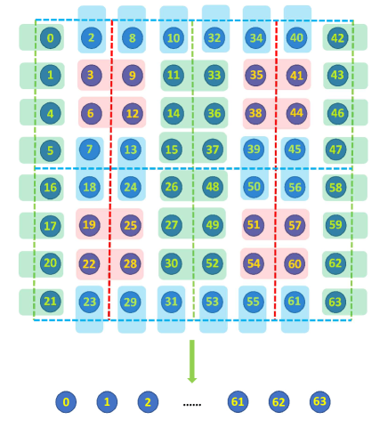
Figure 5: Strategy to put disentanglers in FATTN for a $8\times 8$ lattice. The shadowed bond represents a disentangler. Disentangler with different colors are placed to compensate the violation of the entanglement entropic area law for the cuts with the same colors. And we use numbers to label the physical sites in 2D TTN in a 1D manner. The colored dash lines are the examples of cuts where the 2D TTN can not efficiently capture the entanglement-entropic area-law. See main text for more discussion.

As shown in Fig. 5, We can number the physical indices at the physical layer of the 2D TTN in a one dimensional manner. Using this labeling scheme, we can easily find the cut where the TTN can not capture the entanglement-entropic area law. For a small bond-dimension $D$, examples for cuts where the 2D TTN can not capture the entanglement-entropic area law are shown in the Fig. 5 by colored dash lines. So when augmenting the TTN with disentanglers, we mainly consider these cuts. For concreteness, only periodic boundary conditions are considered in this work.

We firstly consider cuts where the system is divided into two parts with equal number of sites. Fig. 5 shows three ways to bipartite $\mathnormal{A}$ and $\mathnormal{B}$. For the cut with green (blue, red) line, suppose we put $n_{g}(n_{b},n_{r})$ disentanglers cross them, the entanglement entropy along these cuts are:

$$\begin{cases}S_{g}=\log(I_{g})=\log(d^{2n_{g}}D)\\ S_{b}=\log(I_{b})=\log(d^{2n_{b}}D^{2})\\ S_{r}=\log(I_{r})=\log(d^{2n_{r}}D^{4})\end{cases}$$ (7)

As will be discussed below, a constraint that no couple of disentanglers share the same physical index needs to be satisfied to maintain a low computational cost. We also need to keep $I_{g}\approx I_{b}\approx I_{r}$ to make a balance among different cuts to maximize the lowest entanglement entropy with these cuts which means

$$\begin{cases}n_{g}+n_{b}+n_{r}\leq 32\\ n_{g}\geq n_{b}\geq n_{r}\end{cases}$$ (8)

We can set $n_{g}=14,n_{b}=10,n_{r}=8$ (The choice of $n_{g},n_{b},n_{r}$ is not unique. In principle, the optimal choice of them changes with the increase of bond-dimension) and the position for disentanglers is shown in Fig. 5. For an equal bipartition of the $8\times 8$ system, the length of a cut is $16$. So to capture an area law like entanglement entropy $S=16\log k=\log(k^{16})$, the bond-dimensions required by different bipartitions are:

$$\begin{cases}D_{g}=d^{4}(\frac{k}{d^{2}})^{16}\\ D_{b}=d^{6}(\frac{k}{d^{2}})^{8}\\ D_{r}=d^{4}(\frac{k}{d^{2}})^{4}\\ \end{cases}$$ (9)

From Eq. (9) we can see that for $k\leq d^{2}$, with a relatively small bond-dimension, FATTN can capture an area law like entanglement entropy $L\log(d^{2})$. For most of other bipartitions, the entanglement entropy provided in FATTN are also $L\log(d^{2})$ with a similar requirement on $D$ (see the discussion in the Appendix). Comparing with ATTN, the entanglement entropy in FATTN is doubled from $L\log(d)$ to $L\log(d^{2})$ on a finite lattice for most of the cuts with a large $D$. At the same time the computational cost is $O(D^{4}d^{4})$ which is comparable to $O(D^{4}d^{2})$ for ATTN as will be discussed in the next subsection.

IV.2 Optimization of FATTN

Figure 6: In the optimization of disentangler, FATTN can be reduced to a TTN like structure with an SVD. Here we only show the disentanglers which are connected with the considered Hamiltonian term.

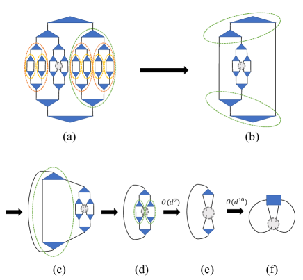
Figure 7: The computation of the environment for disentanglers. The cost of this step is $O(D^{4})$.

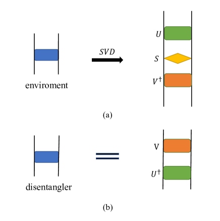
Figure 8: The optimization of disentangler from the corresponding environment tensor, similar as in Eq. (4).

To optimize a FATTN, we need to optimize both the disentanglers and the isometries in it. We follow the procedure in the MERA Evenbly and Vidal (2009b) to optimize disentangler which is very similar to the optimization of isometry in the TTN. First, we calculate the environment for the disentangler we want to optimize. For a Hamiltonian term, we just need to consider the disentanglers which are directly connected to it because other disentanglers can be annihilated because of Eq. (6). As show in Fig. 6, we firstly take a singular value decomposition to get a standard TTN. Then, we contract the TTN to get the environment tensor. This procedure takes a cost of $O(D^{4})$ as shown in Fig. 7. Once we obtain the environment tensor, we follow the strategy in the TTN to get the optimized disentanglers. The details can be found in Fig. 8.

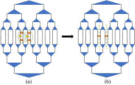
Figure 9: Similar as in Fig. 6, in the optimization of isometry, FATTN can be reduced to a TTN like structure with an SVD. Here we only show the disentanglers which are connected with the considered Hamiltonian term.

The procedure to optimize isometries is similar. For a Hamiltonian term, we only need to consider the disentanglers which are directly connected to it. We contract the Hamiltonian term and the connected disentanglers to get an effective Hamiltonian term in same spirit of ATTN Felser et al. (2021). We then decompose the partial contracted FATTN into a sum of a series of standard TTN as shown in the Fig. 9. After this, we can follow the procedure in the TTN to optimize the isometries in the FATTN.

Overall, for an arbitrary Hamiltonian term, we decompose the relevant disentanglers (for a two-site operator, there are two disentanglers need to be considered in the worst case which causes a factor in the computational cost of $d^{4}$). Then, FATTN becomes a standard TTN. So the overall computational complexity is $O(D^{4}d^{4})$.

V Benchmark results

To show the accuracy of the FATTN, we calculate the ground state energy of the transverse Ising model Suzuki et al. (2013) with the Hamiltonian

$$H_{\rm Ising}=-\sum_{\langle i,j\rangle}\sigma_{i}^{x}\sigma_{j}^{x}-\lambda\sum_{i}\sigma_{i}^{z}$$ (10)

where $\sigma_{x}$ and $\sigma_{z}$ are Pauli matrices and $\lambda$ is the strength of the transverse magnetic field. We consider a $8\times 8$ lattice with periodic boundary conditions where highly accurate numerical results for energy are available for benchmark Tagliacozzo et al. (2009). We focus on $\lambda=3.05$ close to the critical point which is the hard region of this model.

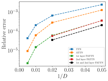
Figure 10: Relative error of the ground state energy per site for different tensor network states ansatzes of the transverse Ising model near the critical point ($\lambda=3.05$) for a $8\times 8$ lattice.

In Fig. 10, we show the relative error of the ground state energy per site as a function of the bond dimension at $\lambda=3.05$ for TTN, ATTN, and FATTN. As expected, FATTN gives the lowest energy with fixed $D$. The error with FATTN is reduced by one (a half) order of magnitude over TTN (ATTN) for all bond dimensions.

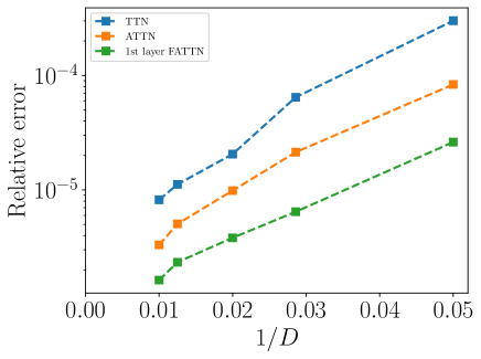
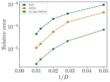
Figure 11: Relative error of the ground state energy per site as a function of bond dimension for different tensor network states ansatzes away from the critical point for a $8\times 8$ lattice. Upper: $\lambda=2$. Down: $\lambda=4$.

The results away from the critical point are shown in Fig. 11. We can see a similar improvement of FATTN over TTN and ATTN for $\lambda=2$ and $4$.

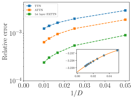
Figure 12: Relative error of the ground state energy per site for different tensor network states ansatzes of the transverse Ising model near the critical point ($\lambda=3.05$) for a $16\times 16$ lattice, compared with the result extrapolated from FATTN data. In the inset, we show the quadratic fit of the FATTN energy and the extrapolated value is $-3.23956(2)$.

For lager systems, we do not have accurate results to compare against. In Fig. 12, we calculate the relative error $\Delta E=|(E_{\rm D}-E_{\rm extra})/E_{\rm extra}|$ of the ground state energy per site for different tensor network ansatzes at different bond-dimension $D$ for a $16\times 16$ lattice. We extrapolate the results calculated by FATTN to obtain $E_{\rm extra}$. We also find a significant improvement in the simulations of FATTN over TTN and ATTN. We notice that the $16\times 16$ FATTN energy with $D=20$ is lower than TTN with $D=100$ while the $8\times 8$ FATTN energy with $D=20$ is comparable with TTN $D=100$.

All of the computations are performed on a single node which contains 2 Intel Xeon Gold 6420R CPUs. For $D=100$, $8\times 8$ lattice case, TTN consumes 25 seconds per sweep while ATTN consumes 60 seconds and FATTN consumes 209 seconds per sweep, which is compatible with the scaling analysis. All the calculations above need about 1 GB RAM per process.

VI Interpolation between TTN and MERA

In the above section, we only place disentanglers at the physical layer of TTN. But this is not the only scheme to augment a TTN. We can place disentanglers at any layer or even at multiple layers of the TTN. The key issue is to keep the computational complexity affordable.

VI.1 Single-layer FATTN

The bond dimension of the disentangler depends on its position in the TTN which determines the upper bound on the entanglement entropy the FATTN can capture. If disentanglers are placed at the physical (first) layer of TTN, the bond dimension of disentangler is $d$ ($d=2$ for spin $1/2$ system) and the entropy the FATTN can mostly encode is $S=L\log(d^{2})$.

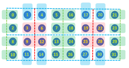
Figure 13: The strategy to place disentanglers in 2nd layer FATTN. Notice that no couple of disentanglers share the same site to ensure a low computational cost.

If we put disentanglers in higher layer, the bond dimension of disentangler is larger than $d$ (to maintain a low cost, we also need to ensure no couple of disentanglers share the same site). But a balance between the bond dimension of disentangler and the maximum number of disentanglers can be placed needs to be reached to provide the maximum entanglement entropy in FATTN. As shown in Fig. 13, we can only place $8^{2}/4$ disentanglers in the second layer of the TTN, but the bond dimension of the disentangler becomes $d^{2}$. So the entanglement entropy can be encoded when placing disentanglers in second layer is the same as the first layer case.

However, when placing disentanglers in higher layer, we find that the entanglement entropy is limited by the red line cuts shown in Fig. 13 or Fig. 5. The entanglement entropy can provide is $S=L/4\log(D)$ if $D<d^{8}$ (for $D>d^{8}$, the entanglement entropy the FATTN can provide is still $L\log(d^{2})$).

Structure	Computational Complexity
1st layer	$O(D^{4}d^{4})$
2nd layer	$O(D^{4}d^{8})$
3rd layer	$O(D^{4}d^{16})$
1st & 2nd layer	$O(D^{4}d^{20})$
ATTN	$O(D^{4}d^{2})$

Table 1: The computational complexity for FATTN with different ways to augment the TTN with disentanglers. The results for ATTN are also listed for comparison.

In TABLE. 1, we list the computational complexity for different types of single-layer FATTN.

VI.2 Multi-layer FATTN

We can also place disentanglers on multiple layers of the TTN. It is easily to show that the FATTN is actually a 2D MERA if disentanglers are placed on every layer of the TTN.

2D MERA can provide an area-law entanglement entropy proportional to $L\log(D)$. But it is highly costly with a computational complexity $O(D^{16})$ Evenbly and Vidal (2009a) which limits the bond dimension can be reached.

To make a balance between cost and entanglement entropy captured in the wave-function ansatz, we can interpolate between single layer FATTN and MERA by placing disentanglers on a relatively small number of layers of the TTN. As an example, we place disentanglers in both the first and second layer of TTN according to Fig. 5 and Fig. 13. The computational complexity are shown in Table. 1.

VI.3 Results for the single-layer FATTN and multi-layer FATTN

In Fig. 10, we show the comparison of the relative error of the ground state energy for different tensor network ansatzes. The system is a $8\times 8$ transverse Ising model with $\lambda=3.05$. The result of 2nd layer FATTN is comparable with 1st layer FATTN, but the 2nd layer FATTN has a higher cost. When placing disentanglers on both the first and second layer, a tiny improvement can be achieved. From Fig. 10, we can find that the best strategy for FATTN is to place the disentanglers at the physical layer according to Fig. 5.

VII Conclusions

In this work, we propose a new tensor network state ansatz FATTN by releasing the unnecessary constraint in ATTN. FATTN can provide an area law like entanglement entropy scaling as $L\log(d^{2})$ for most of the cuts (with a large bond dimension $D$ on a finite lattice) with a low computational cost $O(D^{4}d^{4})$ if the disentanglers are placed on the physical layer. The benchmark results on 2D transverse Ising model near critical point show a large improvement over TTN (nearly one order of magnitude) and ATTN (nearly a half order of magnitude) on the ground state energy. FATTN can be viewed as an interpolation between TTN and MERA to reach a balance between the computational cost and entanglement entropy captured in the wave-function ansatz. Thus, we anticipate FATTN will be an efficient practical numerical tool in the future simulation of two dimensional quantum many-body systems on a finite lattice.

Appendix A The entanglement entropy of FATTN

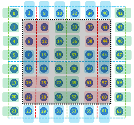
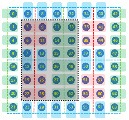
Figure 14: Two cuts for a $8\times 8$ lattice which is not discussed in the main text. There is no disentangler across these cuts in FATTN.

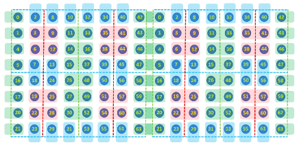
Figure 15: The way to place disentanglers of FATTN on a $8\times 16$ lattice following the strategy in $8\times 8$ lattice in Fig. 5. This strategy can be repeated for the placement of disentanglers in FATTN for larger systems.

In this section, we give a detailed analysis on the entanglement entropy the FATTN can encode. In the main text, we show that the entanglement entropy along the colored dash line in the Fig. 5 is $L\log(d^{2})$. And the requirements for the bond-dimension to encode the entropy of $L\log(k)$ along the colored boundaries are:

$$\begin{cases}D_{g}=d^{4}(\frac{k}{d^{2}})^{16}\\ D_{b}=d^{6}(\frac{k}{d^{2}})^{8}\\ D_{r}=d^{4}(\frac{k}{d^{2}})^{4}\\ \end{cases}$$ (11)

Now, we will show that if these conditions are satisfied, the requirements for most of the other cuts will be also satisfied.

We firstly consider a $8\times 8$ lattice. For the black area shown in the upper panel of Fig. 14 where we do not place any disentangler. The boundary length of the cut is $20$. So in order to encode an entropy of $\log(k^{20})$ the requirement for bond-dimension is:

$$k^{20}=D^{4}d^{20}\Rightarrow D=d^{5}(\frac{k}{d^{2}})^{5}$$ (12)

So once again, we need $k\leq d^{2}$ if we want to use a small bond-dimension $D$ to encode the entanglement-entropic area law of $L\log(d^{2})$.

For the bipartition shown in the down panel of Fig. 14, the requirement for bond-dimension is:

$$k^{16}=D^{2}d^{16}\Rightarrow D=d^{8}(\frac{k}{d^{2}})^{8}$$ (13)

We still need $k\leq d^{2}$ if we want to use a small bond-dimension $D$ to encode the entanglement-entropic area law of $L\log(d^{2})$. For other cuts whose boundary is smaller or there are disentanglers across them, the requirement is also satisfied. So, the FATTN can efficiently encode an entanglement-entropic area law of $L\log(d^{2})$ for a $8\times 8$ lattice.

We can iteratively use the strategies for $8\times 8$ lattice shown in Fig. 5 to analyze larger lattices. In Fig. 15, we take a $16\times 8$ lattice as an example. For a general finite system, the requirement for bond-dimension of an area law as $L\log(k)$ is

$$k^{L}=D^{L/c}d^{L}d^{pL}\Rightarrow D=d^{c(1-p)}(k/d^{2})^{c}$$ (14)

where $pL$($p\in[0,1]$) is the number of disentanglers across the cut and $c$ is a cut dependent constant. Because we place disentanglers across the cuts where c is large, which means $p$ is close to $1$ if $c$ is large. So for most of the cuts $c(1-p)$ is relatively small which means for these cut the captured entanglement entropy scales $L\log(d^{2})$. We can also increase the dimension of the relevant bonds for these cuts with large $c(1-p)$ but maintain a relatively small D for other bonds.

References

- Cabra et al. (2012) D. C. Cabra, A. Honecker, and P. Pujol, Modern Theories of Many-Particle Systems in Condensed Matter Physics, vol. 843 (2012).
- Gang (2007) W. X. Gang, Quantum field theory of many-body systems: from the origin of sound to an origin of light and electrons (Oxford University Press, Oxford, 2007), URL https://cds.cern.ch/record/803748.
- Marino (2017) E. C. Marino, Quantum Field Theory Approach to Condensed Matter Physics (Cambridge University Press, 2017).
- LeBlanc et al. (2015) J. P. F. LeBlanc, A. E. Antipov, F. Becca, I. W. Bulik, G. K.-L. Chan, C.-M. Chung, Y. Deng, M. Ferrero, T. M. Henderson, C. A. Jiménez-Hoyos, et al. (Simons Collaboration on the Many-Electron Problem), Phys. Rev. X 5, 041041 (2015), URL https://link.aps.org/doi/10.1103/PhysRevX.5.041041.
- Loh et al. (1990) E. Y. Loh, J. E. Gubernatis, R. T. Scalettar, S. R. White, D. J. Scalapino, and R. L. Sugar, Phys. Rev. B 41, 9301 (1990), URL https://link.aps.org/doi/10.1103/PhysRevB.41.9301.
- Troyer and Wiese (2005) M. Troyer and U.-J. Wiese, Phys. Rev. Lett. 94, 170201 (2005), URL https://link.aps.org/doi/10.1103/PhysRevLett.94.170201.
- Plenio et al. (2005) M. B. Plenio, J. Eisert, J. Dreißig, and M. Cramer, Phys. Rev. Lett. 94, 060503 (2005), URL https://link.aps.org/doi/10.1103/PhysRevLett.94.060503.
- Vidal et al. (2003) G. Vidal, J. I. Latorre, E. Rico, and A. Kitaev, Phys. Rev. Lett. 90, 227902 (2003), URL https://link.aps.org/doi/10.1103/PhysRevLett.90.227902.
- Srednicki (1993) M. Srednicki, Phys. Rev. Lett. 71, 666 (1993), URL https://link.aps.org/doi/10.1103/PhysRevLett.71.666.
- Eisert et al. (2010) J. Eisert, M. Cramer, and M. B. Plenio, Rev. Mod. Phys. 82, 277 (2010), URL https://link.aps.org/doi/10.1103/RevModPhys.82.277.
- Silvi et al. (2019) P. Silvi, F. Tschirsich, M. Gerster, J. Jünemann, D. Jaschke, M. Rizzi, and S. Montangero, SciPost Phys. Lect. Notes p. 8 (2019), URL https://scipost.org/10.21468/SciPostPhysLectNotes.8.
- Orús (2014) R. Orús, Annals of Physics 349, 117 (2014), ISSN 0003-4916, URL https://www.sciencedirect.com/science/article/pii/S0003491614001596.
- Bridgeman and Chubb (2017) J. C. Bridgeman and C. T. Chubb, Journal of Physics A: Mathematical and Theoretical 50, 223001 (2017), URL https://doi.org/10.1088/1751-8121/aa6dc3.
- Zheng et al. (2017) B.-X. Zheng, C.-M. Chung, P. Corboz, G. Ehlers, M.-P. Qin, R. M. Noack, H. Shi, S. R. White, S. Zhang, and G. K.-L. Chan, Science 358, 1155 (2017), ISSN 0036-8075, eprint http://science.sciencemag.org/content/358/6367/1155.full.pdf, URL http://science.sciencemag.org/content/358/6367/1155.
- Liao et al. (2017) H. J. Liao, Z. Y. Xie, J. Chen, Z. Y. Liu, H. D. Xie, R. Z. Huang, B. Normand, and T. Xiang, Phys. Rev. Lett. 118, 137202 (2017), URL https://link.aps.org/doi/10.1103/PhysRevLett.118.137202.
- White (1993) S. R. White, Phys. Rev. B 48, 10345 (1993), URL https://link.aps.org/doi/10.1103/PhysRevB.48.10345.
- White (1992) S. R. White, Phys. Rev. Lett. 69, 2863 (1992), URL https://link.aps.org/doi/10.1103/PhysRevLett.69.2863.
- Fannes et al. (1992) M. Fannes, B. Nachtergaele, and R. F. Werner, Communications in Mathematical Physics 144, 443 (1992), URL https://doi.org/.
- Stoudenmire and White (2012) E. Stoudenmire and S. R. White, Annual Review of Condensed Matter Physics 3, 111 (2012), eprint https://doi.org/10.1146/annurev-conmatphys-020911-125018, URL https://doi.org/10.1146/annurev-conmatphys-020911-125018.
- Schollwöck (2005) U. Schollwöck, Rev. Mod. Phys. 77, 259 (2005), URL https://link.aps.org/doi/10.1103/RevModPhys.77.259.
- Östlund and Rommer (1995) S. Östlund and S. Rommer, Phys. Rev. Lett. 75, 3537 (1995), URL https://link.aps.org/doi/10.1103/PhysRevLett.75.3537.
- Schollwöck (2011) U. Schollwöck, Annals of Physics 326, 96 (2011), ISSN 0003-4916, january 2011 Special Issue, URL https://www.sciencedirect.com/science/article/pii/S0003491610001752.
- Tagliacozzo et al. (2009) L. Tagliacozzo, G. Evenbly, and G. Vidal, Phys. Rev. B 80, 235127 (2009), URL https://link.aps.org/doi/10.1103/PhysRevB.80.235127.
- Shi et al. (2006) Y.-Y. Shi, L.-M. Duan, and G. Vidal, Phys. Rev. A 74, 022320 (2006), URL https://link.aps.org/doi/10.1103/PhysRevA.74.022320.
- Silvi et al. (2010) P. Silvi, V. Giovannetti, S. Montangero, M. Rizzi, J. I. Cirac, and R. Fazio, Phys. Rev. A 81, 062335 (2010), URL https://link.aps.org/doi/10.1103/PhysRevA.81.062335.
- Gerster et al. (2014) M. Gerster, P. Silvi, M. Rizzi, R. Fazio, T. Calarco, and S. Montangero, Phys. Rev. B 90, 125154 (2014), URL https://link.aps.org/doi/10.1103/PhysRevB.90.125154.
- Cirac et al. (2021) J. I. Cirac, D. Pérez-García, N. Schuch, and F. Verstraete, Rev. Mod. Phys. 93, 045003 (2021), URL https://link.aps.org/doi/10.1103/RevModPhys.93.045003.
- Vanderstraeten et al. (2021) L. Vanderstraeten, L. Burgelman, B. Ponsioen, M. Van Damme, B. Vanhecke, P. Corboz, J. Haegeman, and F. Verstraete, arXiv e-prints arXiv:2110.12726 (2021), eprint 2110.12726.
- Verstraete and Cirac (2004a) F. Verstraete and J. I. Cirac (2004a), eprint cond-mat/0407066.
- Verstraete and Cirac (2004b) F. Verstraete and J. I. Cirac, Phys. Rev. A 70, 060302 (2004b), URL https://link.aps.org/doi/10.1103/PhysRevA.70.060302.
- Verstraete et al. (2006) F. Verstraete, M. M. Wolf, D. Perez-Garcia, and J. I. Cirac, Phys. Rev. Lett. 96, 220601 (2006), URL https://link.aps.org/doi/10.1103/PhysRevLett.96.220601.
- Xie et al. (2014) Z. Y. Xie, J. Chen, J. F. Yu, X. Kong, B. Normand, and T. Xiang, Phys. Rev. X 4, 011025 (2014), URL https://link.aps.org/doi/10.1103/PhysRevX.4.011025.
- Vidal (2008) G. Vidal, Phys. Rev. Lett. 101, 110501 (2008), URL https://link.aps.org/doi/10.1103/PhysRevLett.101.110501.
- Evenbly and Vidal (2009a) G. Evenbly and G. Vidal, Phys. Rev. Lett. 102, 180406 (2009a), URL https://link.aps.org/doi/10.1103/PhysRevLett.102.180406.
- Vidal (2007) G. Vidal, Phys. Rev. Lett. 99, 220405 (2007), URL https://link.aps.org/doi/10.1103/PhysRevLett.99.220405.
- Evenbly and Vidal (2009b) G. Evenbly and G. Vidal, Phys. Rev. B 79, 144108 (2009b), URL https://link.aps.org/doi/10.1103/PhysRevB.79.144108.
- Liang and Pang (1994) S. Liang and H. Pang, Phys. Rev. B 49, 9214 (1994), URL https://link.aps.org/doi/10.1103/PhysRevB.49.9214.
- Jiang et al. (2008) H. C. Jiang, Z. Y. Weng, and T. Xiang, Phys. Rev. Lett. 101, 090603 (2008), URL https://link.aps.org/doi/10.1103/PhysRevLett.101.090603.
- Kalis et al. (2012) H. Kalis, D. Klagges, R. Orús, and K. P. Schmidt, Phys. Rev. A 86, 022317 (2012), URL https://link.aps.org/doi/10.1103/PhysRevA.86.022317.
- Schuch et al. (2007) N. Schuch, M. M. Wolf, F. Verstraete, and J. I. Cirac, Phys. Rev. Lett. 98, 140506 (2007), URL https://link.aps.org/doi/10.1103/PhysRevLett.98.140506.
- Nishino and Okunishi (1996) T. Nishino and K. Okunishi, Journal of the Physical Society of Japan 65, 891 (1996), eprint https://doi.org/10.1143/JPSJ.65.891, URL https://doi.org/10.1143/JPSJ.65.891.
- Xie et al. (2012) Z. Y. Xie, J. Chen, M. P. Qin, J. W. Zhu, L. P. Yang, and T. Xiang, Phys. Rev. B 86, 045139 (2012), URL https://link.aps.org/doi/10.1103/PhysRevB.86.045139.
- foo (a) MERA is constructed with isometries and disentanglers whose definition will be introduced in the main text later.
- Felser et al. (2021) T. Felser, S. Notarnicola, and S. Montangero, Phys. Rev. Lett. 126, 170603 (2021), URL https://link.aps.org/doi/10.1103/PhysRevLett.126.170603.
- foo (b) A detailed analysis of entanglement entropy of FATTN can be found in the appendix. There is a requirement on bond dimension to fulfill the scaling. In this sense, FATTN is designed to study finite systems.
- foo (c) Actually TTN can be constructed from arbitrary rank-3 tensors. But with isometry, the construction becomes trivial.
- Haghshenas (2021) R. Haghshenas, Phys. Rev. Research 3, 023148 (2021), URL https://link.aps.org/doi/10.1103/PhysRevResearch.3.023148.
- Suzuki et al. (2013) S. Suzuki, J.-i. Inoue, and B. K. Chakrabarti, Quantum Ising Phases and Transitions in Transverse Ising Models (Springer Berlin Heidelberg, Berlin, Heidelberg, 2013), pp. 1–11, ISBN 978-3-642-33039-1, URL https://doi.org/10.1007/978-3-642-33039-1_1.
- Gray (2018) J. Gray, Journal of Open Source Software 3, 819 (2018).
- Roberts et al. (2019) C. Roberts, A. Milsted, M. Ganahl, A. Zalcman, B. Fontaine, Y. Zou, J. Hidary, G. Vidal, and S. Leichenauer, Tensornetwork: A library for physics and machine learning (2019), eprint 1905.01330.