Nonlinear Transform Induced Tensor Nuclear Norm for Tensor Completion

Abstract

The linear transform-based tensor nuclear norm (TNN) methods have recently obtained promising results for tensor completion. The main idea of this type of methods is exploiting the low-rank structure of frontal slices of the targeted tensor under the linear transform along the third mode. However, the low-rankness of frontal slices is not significant under linear transforms family. To better pursue the low-rank approximation, we propose a nonlinear transform-based TNN (NTTNN). More concretely, the proposed nonlinear transform is a composite transform consisting of the linear semi-orthogonal transform along the third mode and the element-wise nonlinear transform on frontal slices of the tensor under the linear semi-orthogonal transform, which are indispensable and complementary in the composite transform to fully exploit the underlying low-rankness. Based on the suggested low-rankness metric, i.e., NTTNN, we propose a low-rank tensor completion (LRTC) model. To tackle the resulting nonlinear and nonconvex optimization model, we elaborately design the proximal alternating minimization (PAM) algorithm and establish the theoretical convergence guarantee of the PAM algorithm. Extensive experimental results on hyperspectral images, multispectral images, and videos show that the our method outperforms linear transform-based state-of-the-art LRTC methods qualitatively and quantitatively.

Index terms— Nonlinear transform, tensor nuclear norm, proximal alternating minimization, tensor completion

1 Introduction

With the development of scientific computing, high-dimensional data structure is becoming more and more complicated. As the high-dimensional extension of vectors and matrices, tensors can represent higher-dimensional data, such as hyperspectral images (HSIs) [1, 2], multispectral images (MSIs) [3], and videos [4], which play an increasingly important role in large-scale scientific computing. However, tensor data frequently undergo missing entries or undersample problem due to various unpredictable or unavoidable situations when acquiring it. The problem of recovering missing entries via the observed incomplete tensor is called tensor completion (TC) [5], which is a fundamental problem and has received considerable attention in scientific computing [6, 7, 8, 9]. Generally, multi-dimensional data is internally correlated and the internal redundancy property could be measured by the powerful rank function. Therefore, the low-rank TC (LRTC) problem can be formulated as follows

Figure 1: The pipeline of the linear transform-based TNN method and the proposed NTTNN method on MSI $\mathit{Toy}$ for sampling rate (SR) 10%. (a)The observed incomplete tensor. (b)The transformed tensor under the DFT and the AccEgy with the corresponding percentage of singular values. (c)The recovered tensor by the TNN method and the corresponding pseudo-color image composed of the 1-st, 2-nd, and 5-th bands with the zoom-in region and the corresponding residual part. (d)The transformed tensor under the proposed nonlinear transform $\psi$ and the AccEgy with the corresponding percentage of singular values. (e)The recovered tensor by the NTTNN method and the corresponding pseudo-color image composed of the 1-st, 2-nd, and 5-th bands with the zoom-in region and the corresponding residual part.

$$\min\limits_{\mathcal{X}}\ \textrm{rank}(\mathcal{X})$$

$$\text{s.t. }\ \mathcal{X}_{\Omega}=\mathcal{O}_{\Omega},$$

where, $\mathcal{X}$ and $\mathcal{O}$ denote the required and the observed tensors, respectively, and $\Omega$ is the index set of the observed elements.

However, different from the matrix case, the tensor rank has no unique definition. The CP-rank [10] is defined as the minimum number of rank-one tensors that generate the target tensor, which has been successfully applied in LRTC [11, 12]. However, to determine the CP-rank of the target tensor is NP-hard [13]. The Tucker-rank is defined as a vector constituted of ranks of each mode-$k$ matricization of the tensor. The Tucker-rank has been applied in LRTC problem by minimizing its convex surrogate [14] or non-convex surrogates [15, 16]. Moreover, a series of tensor network decomposition-based ranks are proposed, such as tensor train (TT)-rank [17], tensor ring (TR)-rank [18], and fully-connected tensor network (FCTN)-rank [19]. All of them have been achieved great success in higher-order LRTC [20, 19, 21].

Recently, the tensor tubal-rank [22] has been proposed, which avoids the loss of inherent information in unfolding of the target tensor. Since minimizing the tubal-rank of the target tensor is NP-hard, Zhang $\mathit{et}$ $\mathit{al}.$ [23] proposed a convex surrogate, the tensor nuclear norm (TNN) of underlying tensor, to solve LRTC problem. The TNN-based LRTC model could be mathematically rewritten as

$$\min_{\mathcal{X}}\|\mathcal{X}\|_{\operatorname{TNN}}$$ (1)

$$\text{s.t. }\ \mathcal{X}_{\Omega}=\mathcal{O}_{\Omega},$$

where $\|\mathcal{X}\|_{\operatorname{TNN}}$ is TNN of $\mathcal{X}$ (see Def. 2). Given $\mathcal{X}\in\mathbb{R}^{n_{1}\times{n_{2}}\times{n_{3}}}$, we define $\mathcal{Z}=\mathcal{X}\times_{3}\textbf{F}_{n_{3}}$, where $\textbf{F}_{n_{3}}$ and $\times_{3}$ respectively denotes the Discrete Fourier Transform (DFT) and the mode-3 product of a tensor and a matrix. Since $\textbf{F}_{n_{3}}$ is invertible, we have $\mathcal{X}=\mathcal{Z}\times_{3}\textbf{F}_{n_{3}}^{-1}$. Combining the definition of TNN, the problem (1) is equivalent to the following problem:

$$\min\limits_{\mathcal{Z}}\sum_{i=1}^{n_{3}}\|\mathbf{Z}_{i}\|_{*}$$ (2)

$$\ \text{s.t.}(\mathcal{Z}\times_{3}\textbf{F}_{n_{3}}^{-1})_{\Omega}=\mathcal{O}_{\Omega},$$

where $\textbf{F}_{n_{3}}^{-1}$ denotes the inverse DFT matrix [22], $\|\cdot\|_{*}$ is the matrix nuclear norm, and $\mathbf{Z}_{i}$ denotes $i$-th frontal slice of $\mathcal{Z}$. The problem (LABEL:TNN2) implies that low-tubal-rank structure could be characterized by the summation of nuclear norm of frontal slices under the linear DFT.

Figure 2: The evolution of transform-based TNN methods. The learned transforms are highlighted in boldface, while the other transforms are pre-defined.

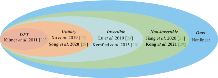
To obtain a better low-rank approximation of frontal slices of the transformed tensor, researchers consider different linear transforms instead of DFT. The discrete cosine transform (DCT) was proposed as an alternatively implemented of DFT in [24, 25], which enjoys less computational cost and obtains a better low-rank approximation compared with DFT. Latterly, Kernfeld $\mathit{et}$ $\mathit{al}.$ [26] and Lu $\mathit{et}$ $\mathit{al}.$ [24] noted that the DFT can be replaced by any invertible transform. Subsequently, Jiang $\mathit{et}$ $\mathit{al}.$ [27] introduced the semi-invertible framelet transform, which broke through the restriction of invertibility compared with invertible transform. It is worth noting that all above mentioned transforms are pre-defined and data-independent. Choosing above transforms are appealing because it is cheap and robust to initialization. Another prominent paradigm is to employ the learning-based methods that further make transforms data-dependent. Song $\mathit{et}$ $\mathit{al}.$ [28] suggested the transform generated by singular values decomposition (SVD) of mode-3 unfolding of the observed tensor. Kong $\mathit{et}$ $\mathit{al}.$ [29] and Jiang $\mathit{et}$ $\mathit{al}.$ [30] further proposed that the observed tensor is used to initialize the transform, which is updated in the algorithm. The above learned methods have shown that the learned transform is flexible for various types of data. The evolution of transform-based TNN methods are summarised in Fig. 2.

Although above transform-based TNN methods have shown effectiveness for LRTC, they still have much room for improvement. Specifically, they pursue the low-rankness of frontal slices of the transformed tensor under a linear transform, which limits their recovered performance especially when sampling rate (SR) is low.

To obtain a better low-rank approximation of frontal slices of the transformed tensor, we propose a nonlinear transform, i.e., $\psi:\mathcal{X}\in\mathbb{R}^{n_{1}\times{n_{2}}\times{n_{3}}}\mapsto\psi(\mathcal{X})\in\mathbb{R}^{n_{1}\times{n_{2}}\times{r}}$. More specifically, $\psi(\mathcal{X})=\phi(\mathcal{X}\times_{3}\mathbf{T})$, where $\times_{3}$ denotes the mode-3 product of the tensor $\mathcal{X}$ and the matrix $\mathbf{T}$ (see Def. 1), $\mathbf{T}\in\mathbb{R}^{r\times{n_{3}}}$ is a learned linear semi-orthogonal transform along the third mode, and $\phi:\mathbf{Z}_{i}\mapsto\phi(\mathbf{Z}_{i})$ is the element-wise nonlinear transform on frontal slices $\mathbf{Z}_{i}(i=1,\cdots,d)$ of the transformed tensor $\mathcal{Z}$ of $\mathcal{X}$ under the linear semi-orthogonal transform $\mathbf{T}$. In the proposed composite transform $\psi$, the learned linear semi-orthogonal transform $\mathbf{T}$ and the element-wise nonlinear transform $\phi$ are indispensable and complementary to fully exploit the underlying low-rankness (we have discussed the indispensability of $\mathbf{T}$ and $\phi$ in the Section 5.2).

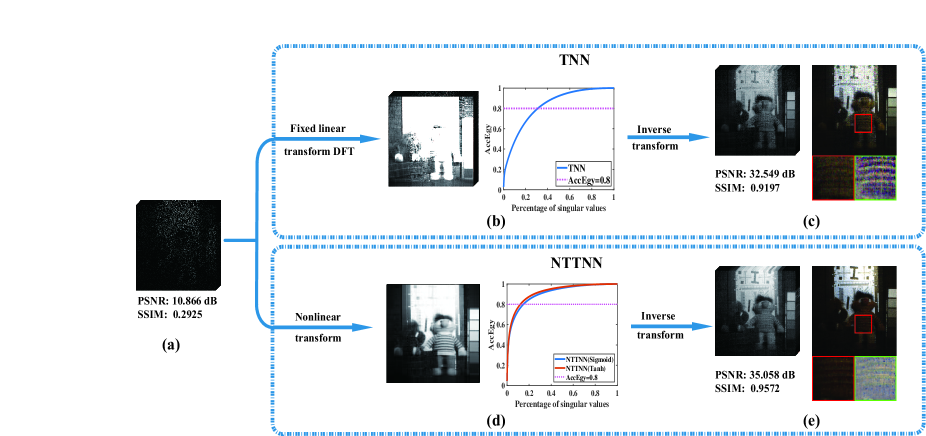
Based on the proposed nonlinear transform, we propose a nonlinear transform-based tensor nuclear norm (NTTNN) to exploit the low-rankness of underlying tensor under the proposed nonlinear transform $\psi$ and establish the corresponding LRTC model. Fig. 1 is the pipeline of the linear transform-based TNN method [23] and the proposed NTTNN method on MSI $\mathit{Toy}$ for SR 10%. From Fig. 1(b) and (d), we can observe that NTTNN with different nonlinear transforms $\phi$ (Tanh and Sigmoid) need less singular values than TNN that is based on linear transform when achieves the same accumulation energy ratio (AccEgy). In other words, the energy of singular values of nonlinear transformed tensor is more concentrated and NTTNN could make the frontal slices of underlying tensor more low-rank. As such, NTTNN can obtain the better low-rank approximation of the underlying tensor under the nonlinear transform $\psi$, which could recover more textures (see zoom-in regions and residual parts between ground truth and recovered tensors) and obtain a better recovered result than TNN, which is demonstrated in Fig. 1(c) and (e). Moreover, the proposed NTTNN is a unified transform-based TNN family, which shows in Fig. 2.

The main contributions of this paper is threefold:

• We propose a nonlinear transformed TNN termed as NTTNN, which could enhance the low-rank approximation of the underlying tensor and can be regarded as a unified transform-based TNN family including many classic transform-based TNN methods.

• Based on NTTNN, we propose the LRTC model and develop an efficient multi-block proximal alternating minimization (PAM) algorithm with theoretical guarantee to solve the resulting model.

• Extensive experiments on HSIs, MSIs, and videos demonstrate that NTTNN outperforms linear transform-based state-of-the-art LRTC methods quantitatively and visually.

The rest part of the paper is arranged as follows. In Section 2, we briefly introduce some essential notations and basic definitions used in this paper. In Section 3, we propose the NTTNN model for LRTC and establish the corresponding algorithm with theoretical convergence guarantee. Section 4 evaluates the performance of the proposed model. Section 5 gives some discussions. Finally, Section 6 concludes this paper.

2 Notations and Preliminaries

In this part, we introduce some basic notations and definitions for developing the proposed nonlinear transform $\psi$ and NTTNN.

The basic notations used in this paper are presented in Table 1.

Table 1: Basic notations.

Notations	Explanations
$\mathit{x}$, $\mathbf{x}$, $\mathbf{X}$, $\mathcal{X}$	Scalar, vector, matrix, tensor.
$x_{ijk}$	The $(i,j,k)$-th element of tensor $\mathcal{X}$.
$\mathcal{X}(:,:,i)$ or $\mathbf{X}_{i}$	The $\mathit{i}$-th frontal slice of tensor $\mathcal{X}$.
$\operatorname{Tr}(\mathbf{X})$	The trace of $\mathbf{X}\in\mathbb{R}^{n\times{n}}$ with $\operatorname{Tr}(\mathbf{X})=\sum_{i=1}^{n}x_{ii}$.
$\left\langle\mathcal{X},\mathcal{Y}\right\rangle$	​ The inner product of ​$\mathcal{X}$ and ​$\mathcal{Y}$ ​ with $\left\langle\mathcal{X},\!\mathcal{Y}\right\rangle\!=\!\sum_{ijk}x_{ijk}y_{ijk}.$
$\|\mathcal{X}\|_{F}$	The Frobenius norm of $\mathcal{X}$ with $\|\mathcal{X}\|_{F}=\sqrt{\left\langle\mathcal{X},\mathcal{X}\right\rangle}$.
$\|\mathbf{X}\|_{*}$	The nuclear norm of $\mathbf{X}$ with $\|\mathbf{X}\|_{*}=\operatorname{Tr}(\sqrt{\mathbf{X}^{\top}\mathbf{X}})$.

Based on above basic notations, we give following definitions:

Definition 1

(mode-$\mathit{k}$ product [31]) The mode-$k$ product of a tensor $\mathcal{Z}$ $\in$ $\mathbb{R}^{n_{1}\times n_{2}\times\cdots\times n_{i}}$ and a matrix $\mathbf{D}$ $\in$ $\mathbb{R}^{h_{i}\times{n_{i}}}$ is defined as

$$\mathcal{X}=\mathcal{Z}\times_{k}\mathbf{D}=\mathtt{fold}_{k}(\mathbf{D}\mathbf{Z}_{(k)}),$$

where $\mathbf{Z}_{(k)}$ is the mode-$k$ matricization of $\mathcal{Z}$ and $\mathtt{fold}_{k}(\cdot)$ is the corresponding inverse operator of matricization that rearranges elements of a matrix into a tensor.

Definition 2

(tensor nuclear norm (TNN) [23]) Let $\mathcal{X}$ $\in$ $\mathbb{R}^{n_{1}\times{n_{2}}\times{n_{3}}}$, the tensor nuclear norm of $\mathcal{X}$ is

$$\|\mathcal{X}\|_{\rm{TNN}}=\sum_{i=1}^{n_{3}}\|\mathbf{{Z}}_{i}\|_{\ast},$$

where $\mathbf{Z}_{i}$ is the $i$-th frontal slice of the transformed tensor $\mathcal{Z}=\mathcal{X}\times_{3}\mathbf{F}_{n_{3}}$.

3 Proposed Model and Solving Algorithm

3.1 Proposed Model

The existing transform-based TNN methods employ linear transform to exploit the low-rankness of frontal slices of the underlying tensor. However, the linear transform does not always make frontal slices of the underlying tensor obviously low-rank, which is shown in Fig. 1(d). To tackle this problem, we propose a nonlinear transform that is defined as

$$\psi(\mathcal{X})=(\phi\circ\mathbf{T})(\mathcal{X})=\phi(\mathcal{X}\times_{3}\mathbf{T}),$$

where, $\mathbf{T}\in\mathbb{R}^{r\times{n_{3}}}$ denotes a learned linear semi-orthogonal transform and satisfies $\mathbf{T}\mathbf{T}^{\top}=\mathbf{I}_{r\times{r}}$, and $\phi:\mathbf{Z}_{i}\mapsto\phi(\mathbf{Z}_{i})$ is the element-wise nonlinear transform on frontal slices $\mathbf{Z}_{i}(i=1,\cdots,d)$ of the transformed tensor $\mathcal{Z}$ of $\mathcal{X}$ under the linear semi-orthogonal transform $\mathbf{T}$.

Remark 1

The introduced nonlinear composed transform, which consists of a nonlinear transform and a learned linear semi-orthogonal transform, can be interpreted as a single layer semi-orthogonal neural network [32, 33]. More specifically, the nonlinear transform is represented by the nonlinear activation function and the linear semi-orthogonal transform corresponds to the semi-orthogonal fully connected layer, where the semi-orthogonality finds to be a favorable property for training deep convolutional neural network [34].

Based on the proposed nonlinear transform, we define the nonlinear transform-based tensor nuclear norm (NTTNN) to exploit the low-rankness of a tensor as follows:

$$\|\mathcal{X}\|_{\rm{NTTNN}}=\left\|\psi(\mathcal{X})\right\|_{*}=\sum_{i=1}^{r}\left\|\phi(\mathbf{Z}_{i})\right\|_{*},$$

where $\mathcal{Z}=\mathcal{X}\times_{3}\mathbf{T}$, $\|\cdot\|_{*}$ denotes the matrix nuclear norm, and $\mathbf{Z}_{i}$ denotes the $i$-th frontal slice of $\mathcal{Z}$. Here, the nonlinear transform $\psi(\cdot)$ could make frontal slices of underlying tensor obviously low-rank, which is shown in Fig. 1(d) that the singular values of $\phi(\mathcal{Z})$ is more concentrated. As a result, the proposed NTTNN could better exploit the low-rankness of latent tensor than TNN-based methods under linear transforms along the third mode.

Based on NTTNN, we propose the following LRTC model:

$$\min_{\mathcal{X},\mathcal{Z},\mathbf{T}}\sum_{i=1}^{r}\left\|\phi(\mathbf{Z}_{i})\right\|_{*}$$ (3)

$$~{}~{}\text{s.t}.~{}~{}~{}\mathcal{X}_{\Omega}=\mathcal{O}_{\Omega},\mathcal{X}=\mathcal{Z}\times_{3}\mathbf{T}^{\top},\mathbf{T}\mathbf{T}^{\top}=\mathbf{I}_{r\times{r}},$$

where, $\mathcal{Z}\in\mathbb{R}^{n_{1}\times n_{2}\times r}$, $\mathbf{T}\in\mathbb{R}^{r\times{n_{3}}}$ is the semi-orthogonal transform, and $\mathbf{I}\in\mathbb{R}^{r\times r}$ is an identity matrix.

Remark 2

NTTNN is a unified transform-based TNN family, which is shown in Fig. 2. More specifically, when the nonlinear function $\phi(\cdot)$ in the proposed transform $\psi(\cdot)$ is defined as $\phi(x)=x$, NTTNN is degraded to previous transform-based TNN methods according to the different $\mathbf{T}$: if $\mathbf{T}$ is the fixed DFT, it is equivalent to the typical TNN method [23]; if $\mathbf{T}$ is the fixed DCT or the fixed framelet transform, it is equivalent to the DCT-based TNN methods [24, 25] or the framelet-based TNN method [27], respectively; if $\mathbf{T}$ is the learned orthogonal transform or the learned semi-orthogonal transform, it is equivalent to the transform-based TNN method [28] or the tensor Q-rank method [29], respectively.

3.2 Solving Algorithm

By introducing indicator functions

$$\Phi(\mathcal{X})=\begin{cases}0,&\mathcal{X}_{\Omega}=\mathcal{O}_{\Omega},\\ +\infty,&\text{otherwise},\end{cases}\begin{aligned} \Psi(\textbf{T})=\begin{cases}0,&\textbf{T}\textbf{T}^{\top}=\textbf{I}_{r\times{r}},\\ +\infty,&\text{otherwise},\end{cases}\end{aligned}$$

the problem (3) can be equivalently rewritten as follows:

$$\min_{\mathcal{X},\mathcal{Z},\textbf{T}}~{}~{}\sum_{i=1}^{r}\left\|\phi(\mathbf{Z}_{i})\right\|_{*}+\Phi(\mathcal{X})+\Psi(\textbf{T})$$ (4)

$$~{}~{}\text{s.t.}~{}~{}~{}~{}~{}\mathcal{X}=\mathcal{Z}\times_{3}{\textbf{T}^{\top}}.$$

To tackle this optimization problem, we introduce the auxiliary variable $\mathcal{Y}=\phi(\mathcal{Z})$ and lean upon the half quadratic splitting [35] tips to transform the constrained problem (4) into the following unconstrained problem:

$$\min_{\mathcal{X},\mathcal{Z},\mathcal{Y},\textbf{T}}~{}~{}\sum_{i=1}^{r}\left\|\mathbf{Y}_{i}\right\|_{*}+\frac{\alpha}{2}\|\mathcal{X}-\mathcal{Z}\times_{3}\textbf{T}^{\top}\|_{F}^{2}+\frac{\beta}{2}\|\mathcal{Y}-\phi(\mathcal{Z})\|_{F}^{2}+\Phi(\mathcal{X})+\Psi(\textbf{T}),$$ (5)

where $\alpha,\beta>0$ are two penalty parameters.

We denote the objective function of problem (5) as $f(\mathcal{X},\mathcal{Y},\mathcal{Z},\textbf{T})$. Under the proximal alternating minimization (PAM) algorithm [36] framework, we can alternatively update each variable:

$$\left\{\begin{aligned} \mathcal{X}^{k+1}\in\ &\operatorname*{argmin}_{\mathcal{X}}\{f(\mathcal{X},\mathcal{Y}^{k},\mathcal{Z}^{k},\textbf{T}^{k})+\frac{\rho_{1}}{2}\|\mathcal{X}-\mathcal{X}^{k}\|_{F}^{2}\},\\ \mathcal{Y}^{k+1}\in\ &\operatorname*{argmin}_{\mathcal{Y}}\{f(\mathcal{X}^{k+1},\mathcal{Y},\mathcal{Z}^{k},\textbf{T}^{k})+\frac{\rho_{2}}{2}\|\mathcal{Y}-\mathcal{Y}^{k}\|_{F}^{2}\},\\ \mathcal{Z}^{k+1}\in\ &\operatorname*{argmin}_{\mathcal{Z}}\{f(\mathcal{X}^{k+1},\mathcal{Y}^{k+1},\mathcal{Z},\textbf{T}^{k})+\frac{\rho_{3}}{2}\|\mathcal{Z}-\mathcal{Z}^{k}\|_{F}^{2}\},\\ \textbf{T}^{k+1}\in\ &\operatorname*{argmin}_{\textbf{T}}\{f(\mathcal{X}^{k+1},\mathcal{Y}^{k+1},\mathcal{Z}^{k+1},\textbf{T})+\frac{\rho_{4}}{2}\|\textbf{T}-\textbf{T}^{k}\|_{F}^{2}\},\\ \end{aligned}\right.$$ (6)

where $\rho_{1}$, $\rho_{2}$, $\rho_{3}$, and $\rho_{4}$ are four positive constants, and $k$ denotes the iteration number. Next, we give details for updating the subproblems about $\mathcal{X}$, $\mathcal{Y}$, $\mathcal{Z}$, and T.

$\bullet$ Updating $\mathcal{X}$ subproblem

The $\mathcal{X}$ subproblem is

$$\operatorname*{argmin}_{\mathcal{X}}\frac{\alpha}{2}\|\mathcal{X}-\mathcal{Z}^{k}\times_{3}{\textbf{T}^{k}}^{\top}\|_{F}^{2}+\frac{\rho_{1}}{2}\|\mathcal{X}-\mathcal{X}^{k}\|_{F}^{2}+\Phi(\mathcal{X}).$$ (7)

The closed-form solution of the problem (7) is

$$\mathcal{X}^{k+1}=\left(\frac{\alpha\mathcal{Z}^{k}\times_{3}{\textbf{T}^{k}}^{\top}+\rho_{1}\mathcal{X}^{k}}{\alpha+\rho_{1}}\right)_{\Omega^{c}}+\mathcal{O}_{\Omega},$$ (8)

where $\Omega^{c}$ denotes the complement set of $\Omega$.

$\bullet$ Updating $\mathcal{Y}$ subproblem

The $\mathcal{Y}$ subproblem is

$$\operatorname*{argmin}_{\mathcal{Y}}\sum_{i=1}^{r}\left\|\mathbf{Y}_{i}\right\|_{*}+\frac{\beta}{2}\|\mathcal{Y}-\phi(\mathcal{Z}^{k})\|_{F}^{2}+\frac{\rho_{2}}{2}\|\mathcal{Y}-\mathcal{Y}^{k}\|_{F}^{2}.$$

The $\mathcal{Y}$ subproblem can be decomposed into the following $r$ subproblems:

$$\operatorname*{argmin}_{\textbf{Y}_{i}}\|\textbf{Y}_{i}\|_{*}+\frac{\beta+\rho_{2}}{2}\|\textbf{Y}_{i}-\mathbf{H}_{i}\|_{F}^{2},$$ (9)

where $\mathbf{H}^{k}_{i}=\frac{\beta\phi(\textbf{Z}^{k}_{i})+\rho_{2}\textbf{Y}^{k}_{i}}{\beta+\rho_{2}}$. By employing singular value thresholding (SVT) operator [37], the closed-form solution of each subproblem (9) is

$$\textbf{Y}^{k+1}_{i}=\mathcal{T}_{\frac{1}{\beta+\rho_{2}}}(\mathbf{H}^{k}_{i})=\hat{\textbf{U}}\mathcal{T}_{\frac{1}{\beta+\rho_{2}}}(\hat{\textbf{D}})\hat{\textbf{V}}^{\top},$$ (10)

where $(\hat{\textbf{U}},\hat{\textbf{D}},\hat{\textbf{V}})$ are derived from SVD of $\mathbf{H}^{k}_{i}$ and $\mathcal{T}_{\frac{1}{\beta+\rho}}(\hat{\textbf{D}})=\mathtt{diag}(\operatorname{max}(\sigma_{j}-\frac{1}{\beta+\rho_{2}},0))$.

$\bullet$ Updating $\mathcal{Z}$ subproblem

The $\mathcal{Z}$ subproblem is

$$\operatorname*{argmin}_{\mathcal{Z}}~{}\frac{\alpha}{2}\|\mathcal{X}^{k+1}-\mathcal{Z}\times_{3}{\textbf{T}^{k}}^{\top}\|_{F}^{2}+\frac{\beta}{2}\|\mathcal{Y}^{k+1}-\phi(\mathcal{Z})\|_{F}^{2}+\frac{\rho_{3}}{2}\|\mathcal{Z}-\mathcal{Z}^{k}\|_{F}^{2}.$$

The $\mathcal{Z}$ subproblem can be equivalently formulated as follows:

$$\operatorname*{argmin}_{\textbf{Z}_{(3)}}~{}\frac{\alpha}{2}\|\textbf{Z}_{(3)}-{\textbf{T}^{k}}\textbf{X}^{k+1}_{(3)}\|_{F}^{2}+\frac{\beta}{2}\|\phi(\textbf{Z}_{(3)})-\textbf{Y}^{k+1}_{(3)}\|_{F}^{2}+\frac{\rho_{3}}{2}\|\textbf{Z}_{(3)}-\textbf{Z}^{k}_{(3)}\|_{F}^{2}$$ (11)

$$=\operatorname*{argmin}_{\textbf{Z}_{(3)}}~{}\frac{\alpha+\rho_{3}}{2}\|\textbf{Z}_{(3)}-\mathbf{G}^{k}\|_{F}^{2}+\frac{\beta}{2}\|\phi(\textbf{Z}_{(3)})-\textbf{Y}^{k+1}_{(3)}\|_{F}^{2},$$

where $\textbf{G}^{k}=\frac{\alpha{\textbf{T}^{k}}\textbf{X}^{k+1}_{(3)}+\rho_{3}\textbf{Z}^{k}_{(3)}}{\alpha+\rho_{3}}$. We denote the $(i,j)$-th element of $\mathbf{Z}^{k}_{(3)}$, $\mathbf{G}^{k}$, and $\mathbf{Y}^{k}_{(3)}$ as $z_{ij}^{k}=\mathbf{Z}^{k}_{(3)}(i,j)$, $g^{k}_{ij}=\mathbf{G}^{k}(i,j)$, and $y^{k}_{ij}=\mathbf{Y}^{k}_{(3)}(i,j)$, respectively. Then, the problem (11) can be decomposed into $n_{1}n_{2}r$ one-dimensional nonlinear equations as follows:

$$\operatorname*{argmin}_{z_{ij}}~{}\frac{\alpha+\rho_{3}}{2}(z_{ij}-g^{k}_{ij})^{2}+\frac{\beta}{2}(\phi(z_{ij})-y^{k+1}_{ij})^{2},$$ (12)

which can be solved by the Newton method.

$\bullet$ Updating T subproblem

The T subproblem is

$$\operatorname*{argmin}_{\textbf{T}}~{}\frac{\alpha}{2}\|\mathcal{X}^{k+1}-\mathcal{Z}^{k+1}\times_{3}\textbf{T}^{\top}\|_{F}^{2}+\frac{\rho_{4}}{2}\|\textbf{T}-\textbf{T}^{k}\|_{F}^{2}+\Psi(\textbf{T}).$$ (13)

Note that the problem (13) can be equivalently transformed the following problem:

$$\operatorname*{argmin}_{\textbf{T}}~{}\frac{\alpha}{2}\|\mathcal{X}^{k+1}-\mathcal{Z}^{k+1}\times_{3}\textbf{T}^{\top}\|_{F}^{2}+\frac{\rho_{4}}{2}\|\textbf{T}-\textbf{T}^{k}\|_{F}^{2}+\Psi(\textbf{T})$$ (14)

$$= \operatorname*{argmin}_{\textbf{T}}~{}\frac{\alpha}{2}\|\textbf{X}_{(3)}^{k+1}-\textbf{T}^{\top}\textbf{Z}_{(3)}^{k+1}\|_{F}^{2}+\frac{\rho_{4}}{2}\|\textbf{T}-\textbf{T}^{k}\|_{F}^{2}+\Psi(\textbf{T})$$

$$= \operatorname*{argmin}_{\textbf{T}}~{}\frac{\alpha}{2}\operatorname{Tr}[(\textbf{X}_{(3)}^{k+1}-\textbf{T}^{\top}\textbf{Z}_{(3)}^{k+1})^{\top}(\textbf{X}_{(3)}^{k+1}-\textbf{T}^{\top}\textbf{Z}_{(3)}^{k+1})]$$

$$~{}~{}~{}~{}~{}~{}~{}~{}~{}~{}~{}+\frac{\rho_{4}}{2}\operatorname{Tr}[(\textbf{T}-\textbf{T}^{k})^{\top}(\textbf{T}-\textbf{T}^{k})]+\Psi(\textbf{T})$$

$$= \operatorname*{argmax}_{\textbf{T}}~{}\operatorname{Tr}[(\alpha\textbf{X}_{(3)}^{k+1}(\textbf{Z}_{(3)}^{k+1})^{\top}+\rho_{4}{\textbf{T}^{k}}^{\top})\textbf{T}]-\Psi(\textbf{T}),$$

where $\operatorname{Tr}(\mathbf{X})$ denotes the trace of matrix $\mathbf{X}$. Supposing the SVD of $\alpha\textbf{X}_{(3)}^{k+1}(\textbf{Z}_{(3)}^{k+1})^{\top}+\rho_{4}{\textbf{T}^{k}}^{\top}$ is $\tilde{\textbf{U}}\tilde{\textbf{D}}\tilde{\textbf{V}}^{\top}$, we have

$$\operatorname{Tr}(\tilde{\textbf{U}}\tilde{\textbf{D}}\tilde{\textbf{V}}^{\top}\textbf{T})=\operatorname{Tr}(\tilde{\textbf{D}}\tilde{\textbf{U}}\tilde{\textbf{V}}^{\top}\textbf{T}).$$

Since $\tilde{\textbf{D}}$ is the diagonal matrix, the maximization problem in (LABEL:Tmax) can be maximized when the diagonal elements of $\tilde{\textbf{U}}\tilde{\textbf{V}}^{\top}\textbf{T}$ is positive and maximum. By the Cauchy-Schwartz inequality, this is achieved when $\textbf{T}=(\tilde{\textbf{U}}\tilde{\textbf{V}}^{\top})^{\top}$ in which case the diagonal elements are all 1. Hence the closed-form solution of (13) is

$$\textbf{T}^{k+1}=\tilde{\textbf{V}}\tilde{\textbf{U}}^{\top},$$ (15)

where $\tilde{\textbf{U}}$ and $\tilde{\textbf{V}}$ are the orthogonal matrices obtained by the following SVD:

$$\alpha\textbf{X}_{(3)}^{k+1}(\textbf{Z}_{(3)}^{k+1})^{\top}+\rho_{4}{\textbf{T}^{k}}^{\top}=\tilde{\textbf{U}}\tilde{\textbf{D}}\tilde{\textbf{V}}^{\top}.$$

We summary the solving algorithm for NTTNN in Algorithm 1.

Algorithm 1 The PAM-based solver for the proposed NTTNN model.

Input: The observed $\mathcal{O}\in\mathbb{R}^{n_{1}\times{n_{2}}\times{n_{3}}}$ , index set $\Omega$, the row number $r$ of the transform $\mathbf{T}$, proximal parameters $\alpha$, $\beta$, and $\rho_{i}(i=1,\cdots,4)$.

Output: The recovered third-order tensor $\mathcal{X}$.

Initialization: $\mathcal{X}^{0}$, $\mathcal{Y}^{0}$, $\mathcal{Z}^{0}$, T⁰;

While $\frac{\left\|\mathcal{X}^{k+1}-\mathcal{X}^{k}\right\|_{F}}{\left\|\mathcal{X}^{k}\right\|_{F}}\leq 10^{-4}$ do

          Update $\mathcal{X}^{k+1}$ via (8);

          Update $\mathcal{Y}^{k+1}$ via (10);

          Update $\mathcal{Z}^{k+1}$ via (12);

          Update T^k+1 via (15);

end while

3.3 Convergence analysis

Under the PAM algorithm framework, we establish the global convergence guarantee of Algorithm 1 to solve (5). First of all, we denote following functions:

$$f(\mathcal{X},\mathcal{Y},\mathcal{Z},\textbf{T})=\sum_{i=1}^{r}\left\|\mathbf{Y}_{i}\right\|_{*}+\frac{\alpha}{2}\|\mathcal{X}-\mathcal{Z}\times_{3}\textbf{T}^{\top}\|_{F}^{2}+\frac{\beta}{2}\|\mathcal{Y}-\phi(\mathcal{Z})\|_{F}^{2}+\Phi(\mathcal{X})+\Psi(\textbf{T}),$$

and

$$f_{1}(\mathcal{X},\mathcal{Y},\mathcal{Z},\textbf{T})=\frac{\alpha}{2}\|\mathcal{X}-\mathcal{Z}\times_{3}\textbf{T}^{\top}\|_{F}^{2}+\frac{\beta}{2}\|\mathcal{Y}-\phi(\mathcal{Z})\|_{F}^{2}.$$

First, we introduce the necessary ingredients used for the convergence analysis.

Definition 3

(Kurdyka-Łojasiewicz property[38]). The function $\psi(x):\mathbb{R}^{n}\rightarrow\mathbb{R}\cup+\infty$ is said to have the Kurdyka-$\L$ojasiewicz (K-Ł) property at $x^{*}\in\operatorname{dom}(\partial\psi(x))$ if there exist $\eta\in(0,+\infty]$, a neighborhood $U$ of $x^{*}$ and a continuous concave function $\psi(x):[0,\eta)\rightarrow\mathbb{R}_{+}$ satisfy:

• $\psi(0)=0$,

• $\psi(x)$ is $C^{1}$ on $(0,\eta]$,

• for any $x\in(0,\eta),\psi^{\prime}(x)>0$,

• for any $x$ in $U\cap[\psi(x^{*})<\psi(x)<\psi(x^{*})+\eta]$

The proper lower semi-continuous functions are called K-Ł functions, if they satisfy K-Ł property at each point of $\operatorname{dom}(\partial\psi(x))$.

Definition 4

(Semi-algebraic set and semi-algebraic function[38]) If there exists a series of real polynomial functions $m_{ij}$ and $n_{ij}$ satisfy $S=\cap_{j}\cup_{i}\{x\in\mathbb{R}^{n}:m_{ij}(x)=0,n_{ij}(x)<0\},$ then the subset $S\in\mathbb{R}$ is a semi-algebraic set. If the graph $\{(x,y)\in\mathbb{R}^{n}\times\mathbb{R},f(x)=y\}$ of the function $f$ is a semi-algebraic set, then $f$ is a semi-algebraic function.

Remark 3

A semi-algebraic real valued function $f$ satisfies K-Ł property at each $x\in\operatorname{dom}(f)$, i.e., $f$ is a K-Ł function.

Lemma 1

(Sufficient decrease lemma). For any $\rho_{i}>0$ $(i=1,2,3,4)$, the sequence $\{\mathcal{X}^{k},\mathcal{Y}^{k},\mathcal{Z}^{k},\mathbf{T}^{k}\}$ that is generated by (6) satisfies the following formulae:

$$\left\{\begin{aligned} &f(\mathcal{X}^{k+1},\mathcal{Y}^{k},\mathcal{Z}^{k},\mathbf{T}^{k})+\frac{\rho_{1}}{2}\|\mathcal{X}^{k+1}-\mathcal{X}^{k}\|_{F}^{2}\leq f(\mathcal{X}^{k},\mathcal{Y}^{k},\mathcal{Z}^{k},\mathbf{T}^{k}),\\ &f(\mathcal{X}^{k+1},\mathcal{Y}^{k+1},\mathcal{Z}^{k},\mathbf{T}^{k})+\frac{\rho_{2}}{2}\|\mathcal{Y}^{k+1}-\mathcal{Y}^{k}\|_{F}^{2}\leq f(\mathcal{X}^{k+1},\mathcal{Y}^{k},\mathcal{Z}^{k},\mathbf{T}^{k}),\\ &f(\mathcal{X}^{k+1},\mathcal{Y}^{k+1},\mathcal{Z}^{k+1},\mathbf{T}^{k})+\frac{\rho_{3}}{2}\|\mathcal{Z}^{k+1}-\mathcal{Z}^{k}\|_{F}^{2}\leq f(\mathcal{X}^{k+1},\mathcal{Y}^{k+1},\mathcal{Z}^{k},\mathbf{T}^{k}),\\ &f(\mathcal{X}^{k+1},\mathcal{Y}^{k+1},\mathcal{Z}^{k+1},\mathbf{T}^{k+1})+\frac{\rho_{4}}{2}\|\mathbf{T}^{k+1}-\mathbf{T}^{k}\|_{F}^{2}\leq f(\mathcal{X}^{k+1},\mathcal{Y}^{k+1},\mathcal{Z}^{k+1},\mathbf{T}^{k}).\end{aligned}\right.$$ (16)

Proof.  Let $\mathcal{X}^{k+1}$, $\mathcal{Y}^{k+1}$, $\mathcal{Z}^{k+1}$, and $\textbf{T}^{k+1}$ be optimal solutions of the corresponding subproblem in (6), then we have

$$\left\{\begin{aligned} &f(\mathcal{X}^{k+1},\mathcal{Y}^{k},\mathcal{Z}^{k},\mathbf{T}^{k})+\frac{\rho_{1}}{2}\|\mathcal{X}^{k+1}-\mathcal{X}^{k}\|_{F}^{2}\leq f(\mathcal{X}^{k},\mathcal{Y}^{k},\mathcal{Z}^{k},\mathbf{T}^{k}),\\ &f(\mathcal{X}^{k+1},\mathcal{Y}^{k+1},\mathcal{Z}^{k},\mathbf{T}^{k})+\frac{\rho_{2}}{2}\|\mathcal{Y}^{k+1}-\mathcal{Y}^{k}\|_{F}^{2}\leq f(\mathcal{X}^{k+1},\mathcal{Y}^{k},\mathcal{Z}^{k},\mathbf{T}^{k}),\\ &f(\mathcal{X}^{k+1},\mathcal{Y}^{k+1},\mathcal{Z}^{k+1},\mathbf{T}^{k})+\frac{\rho_{3}}{2}\|\mathcal{Z}^{k+1}-\mathcal{Z}^{k}\|_{F}^{2}\leq f(\mathcal{X}^{k+1},\mathcal{Y}^{k+1},\mathcal{Z}^{k},\mathbf{T}^{k}),\\ &f(\mathcal{X}^{k+1},\mathcal{Y}^{k+1},\mathcal{Z}^{k+1},\mathbf{T}^{k+1})+\frac{\rho_{4}}{2}\|\mathbf{T}^{k+1}-\mathbf{T}^{k}\|_{F}^{2}\leq f(\mathcal{X}^{k+1},\mathcal{Y}^{k+1},\mathcal{Z}^{k+1},\mathbf{T}^{k}).\end{aligned}\right.$$

The proof of the sufficient decrease lemma is completed. $\square$

Lemma 2

(Relative error lemma). Assuming that $\phi(\cdot)$ is a real analytic function, and continuous on its domain with Lipschitz continuous on any bounded set. Then, the sequence $\{\mathcal{X}^{k},\mathcal{Y}^{k},\mathcal{Z}^{k},\mathbf{T}^{k}\}$ obtained by (6) is bounded, and for any $\rho_{i}>0$ $(i=1,2,3,4)$, there exist $V_{i}^{t+1}$ such that $\{\mathcal{X}^{k},\mathcal{Y}^{k},\mathcal{Z}^{k},\mathbf{T}^{k}\}$ satisfies the following formulae:

$$\left\{\begin{aligned} &\|V_{1}^{k+1}+\nabla_{\mathcal{X}}f_{1}(\mathcal{X}^{k+1},\mathcal{Y}^{k},\mathcal{Z}^{k},\mathbf{T}^{k})\|_{F}\leq\rho_{1}\|\mathcal{X}^{k+1}-\mathcal{X}^{k}\|_{F},\\ &\|V_{2}^{k+1}+\nabla_{\mathcal{Y}}f_{1}(\mathcal{X}^{k+1},\mathcal{Y}^{k+1},\mathcal{Z}^{k},\mathbf{T}^{k})\|_{F}\leq\rho_{2}\|\mathcal{Y}^{k+1}-\mathcal{Y}^{k}\|_{F},\\ &\|V_{3}^{k+1}+\nabla_{\mathcal{Z}}f_{1}(\mathcal{X}^{k+1},\mathcal{Y}^{k+1},\mathcal{Z}^{k+1},\mathbf{T}^{k})\|_{F}\leq\rho_{3}\|\mathcal{Z}^{k+1}-\mathcal{Z}^{k}\|_{F},\\ &\|V_{4}^{k+1}+\nabla_{\mathbf{T}}f_{1}(\mathcal{X}^{k+1},\mathcal{Y}^{k+1},\mathcal{Z}^{k+1},\mathbf{T}^{k+1})\|_{F}\leq\rho_{4}\|\mathbf{T}^{k+1}-\mathbf{T}^{k}\|_{F}.\end{aligned}\right.$$ (17)

Proof.  Firstly, we prove $\{\mathcal{X}^{k},\mathcal{Y}^{k},\mathcal{Z}^{k},\mathbf{T}^{k}\}$ obtained by (6) is bounded. Since

$$\lim_{\|\mathcal{X}\|_{F}\rightarrow+\infty}\frac{\alpha}{2}\|\mathcal{X}-\mathcal{Z}\times_{3}\mathbf{T}^{\top}\|_{F}=+\infty,~{}~{}~{}\lim_{\|\mathcal{Y}\|_{F}\rightarrow+\infty}\sum_{i=1}^{r}\left\|\mathbf{Y}_{i}\right\|_{*}=+\infty,$$

$$\lim_{\|\mathcal{Z}\|_{F}\rightarrow+\infty}\frac{\alpha}{2}\|\mathcal{X}-\mathcal{Z}\times_{3}\mathbf{T}^{\top}\|_{F}=+\infty,~{}~{}~{}\lim_{\|\mathbf{T}\|_{F}\rightarrow+\infty}\Psi(\mathbf{T})=+\infty,$$

we can respectively obtain

$$\lim_{\|\mathcal{X}\|_{F}\rightarrow+\infty}f(\mathcal{X},\mathcal{Y},\mathcal{Z},\mathbf{T})=+\infty,\lim_{\|\mathcal{Y}\|_{F}\rightarrow+\infty}f(\mathcal{X},\mathcal{Y},\mathcal{Z},\mathbf{T})=+\infty,$$

$$\lim_{\|\mathcal{Z}\|_{F}\rightarrow+\infty}f(\mathcal{X},\mathcal{Y},\mathcal{Z},\mathbf{T})=+\infty,\lim_{\|\mathbf{T}\|_{F}\rightarrow+\infty}f(\mathcal{X},\mathcal{Y},\mathcal{Z},\mathbf{T})=+\infty.$$

Therefore, we have the conclusion that $f(\mathcal{X}^{k+1},\mathcal{Y}^{k+1},\mathcal{Z}^{k+1},\mathbf{T}^{k+1})$ would approach infinity if $\{\mathcal{X}^{k},\mathcal{Y}^{k},\mathcal{Z}^{k},\mathbf{T}^{k}\}$ is unbounded, i.e., the sequence $\{\mathcal{X}^{k},\mathcal{Y}^{k},\mathcal{Z}^{k},\mathbf{T}^{k}\}$ is bounded if $f(\mathcal{X}^{k+1},\mathcal{Y}^{k+1},\mathcal{Z}^{k+1},$ $\mathbf{T}^{k+1})$ is finite. Thus, we proof $f(\mathcal{X}^{k+1},\mathcal{Y}^{k+1},\mathcal{Z}^{k+1},$ $\mathbf{T}^{k+1})$ is finite in the following. According to Lemma 16, we have

$$f(\mathcal{X}^{k+1},\mathcal{Y}^{k+1},\mathcal{Z}^{k+1},\mathbf{T}^{k+1}) \leq f(\mathcal{X}^{k+1},\mathcal{Y}^{k+1},\mathcal{Z}^{k+1},\mathbf{T}^{k+1})+\frac{\rho_{1}}{2}\|\mathcal{X}^{k+1}-\mathcal{X}^{k}\|_{F}^{2}+\frac{\rho_{2}}{2}\|\mathcal{Y}^{k+1}-\mathcal{Y}^{k}\|_{F}^{2}$$

$$+\frac{\rho_{3}}{2}\|\mathcal{Z}^{k+1}-\mathcal{Z}^{k}\|_{F}^{2}+\frac{\rho_{4}}{2}\|\mathbf{T}^{k+1}-\mathbf{T}^{k}\|_{F}^{2}$$

$$\leq f(\mathcal{X}^{k},\mathcal{Y}^{k},\mathcal{Z}^{k},\mathbf{T}^{k})$$

$$\leq f(\mathcal{X}^{k},\mathcal{Y}^{k},\mathcal{Z}^{k},\mathbf{T}^{k})+\frac{\rho_{1}}{2}\|\mathcal{X}^{k}-\mathcal{X}^{k-1}\|_{F}^{2}+\frac{\rho_{2}}{2}\|\mathcal{Y}^{k}-\mathcal{Y}^{k-1}\|_{F}^{2}$$

$$+\frac{\rho_{3}}{2}\|\mathcal{Z}^{k}-\mathcal{Z}^{k-1}\|_{F}^{2}+\frac{\rho_{4}}{2}\|\mathbf{T}^{k}-\mathbf{T}^{k-1}\|_{F}^{2}$$

$$\leq$$

$$\cdots$$

$$\leq f(\mathcal{X}^{0},\mathcal{Y}^{0},\mathcal{Z}^{0},\mathbf{T}^{0}),$$

then $f(\mathcal{X}^{k+1},\mathcal{Y}^{k+1},\mathcal{Z}^{k+1},\mathbf{T}^{k+1})$ is finite.

Therefore, we can conclude that $\{\mathcal{X}^{k},\mathcal{Y}^{k},\mathcal{Z}^{k},\mathbf{T}^{k}\}$ obtained by (6) is bounded.

Next, let $\mathcal{X}^{k+1}$, $\mathcal{Y}^{k+1}$, $\mathcal{Z}^{k+1}$, and $\mathbf{T}^{k+1}$ be optimal solutions of each subproblem in (6). For $\mathcal{X}$, $\mathcal{Y}$, and $\mathbf{T}$ subproblems, we have

$$\left\{\begin{aligned} &0\in\partial\Phi(\mathcal{X}^{k+1})+\alpha(\mathcal{X}^{k+1}-\mathcal{Z}^{k}\times_{3}{\mathbf{T}^{k}}^{\top})+\rho_{1}(\mathcal{X}^{k+1}-\mathcal{X}^{k}),\\ &0\in\partial(\sum_{i=1}^{r}\left\|\mathbf{Y}^{k+1}_{i}\right\|_{*})+\beta(\mathcal{Y}^{k+1}-\phi(\mathcal{Z}^{k}))+\rho_{2}(\mathcal{Y}^{k+1}-\mathcal{Y}^{k}),\\ &0\in\partial\Psi(\mathbf{T}^{k+1})-\alpha(\mathbf{X}^{k+1}_{(3)}-{\mathbf{T}^{k+1}}^{\top}\mathbf{Z}_{(3)}^{k+1})\mathbf{Z}^{k+1}_{(3)}+\rho_{4}(\mathbf{T}^{k+1}-\mathbf{T}^{k}).\end{aligned}\right.$$

Then we can define $V_{1}$, $V_{2}$, and $V_{4}$ as

$$\left\{\begin{aligned} &V_{1}^{k+1}=-\alpha(\mathcal{X}^{k+1}-\mathcal{Z}^{k}\times_{3}{\mathbf{T}^{k}}^{\top})-\rho_{1}(\mathcal{X}^{k+1}-\mathcal{X}^{k}),\\ &V_{2}^{k+1}=-\beta(\mathcal{Y}^{k+1}-\phi(\mathcal{Z}^{k}))-\rho_{2}(\mathcal{Y}^{k+1}-\mathcal{Y}^{k}),\\ &V_{4}^{k+1}=\alpha(\mathbf{X}^{k+1}_{(3)}-{\mathbf{T}^{k+1}}^{\top}\mathbf{Z}_{(3)}^{k+1})\mathbf{Z}^{k+1}_{(3)}-\rho_{4}(\mathbf{T}^{k+1}-\mathbf{T}^{k}).\end{aligned}\right.$$

Additionally, from the subproblem (12), we have

$$0\in(\alpha+\rho_{3})(z_{ij}^{k+1}-g_{ij}^{k})+\beta\partial\phi(z_{ij}^{k+1})(\phi(z_{ij}^{k+1})-y_{ij}^{k+1}),$$

thus we can define $V_{3}^{k+1}=0$. Since $\phi(\cdot)$ is a real analytic function, and continuous on its domain with Lipschitz continuous on any bounded set, $\nabla f_{1}$ is Lipschitz continuous on any bounded set. Since $\{\mathcal{X}^{k},\mathcal{Y}^{k},\mathcal{Z}^{k},\mathbf{T}^{k}\}$ is bounded and $\nabla f_{1}$ is Lipschitz continuous on any bounded set, then for any $\rho_{i}>0$, the following formulae holds:

$$\left\{\begin{aligned} &\|V_{1}^{k+1}+\nabla_{\mathcal{X}}f_{1}(\mathcal{X}^{k+1},\mathcal{Y}^{k},\mathcal{Z}^{k},\mathbf{T}^{k})\|_{F}\leq\rho_{1}\|\mathcal{X}^{k+1}-\mathcal{X}^{k}\|_{F},\\ &\|V_{2}^{k+1}+\nabla_{\mathcal{Y}}f_{1}(\mathcal{X}^{k+1},\mathcal{Y}^{k+1},\mathcal{Z}^{k},\mathbf{T}^{k})\|_{F}\leq\rho_{2}\|\mathcal{Y}^{k+1}-\mathcal{Y}^{k}\|_{F},\\ &\|V_{3}^{k+1}+\nabla_{\mathcal{Z}}f_{1}(\mathcal{X}^{k+1},\mathcal{Y}^{k+1},\mathcal{Z}^{k+1},\mathbf{T}^{k})\|_{F}\leq\rho_{3}\|\mathcal{Z}^{k+1}-\mathcal{Z}^{k}\|_{F},\\ &\|V_{4}^{k+1}+\nabla_{\mathbf{T}}f_{1}(\mathcal{X}^{k+1},\mathcal{Y}^{k+1},\mathcal{Z}^{k+1},\mathbf{T}^{k+1})\|_{F}\leq\rho_{4}\|\mathbf{T}^{k+1}-\mathbf{T}^{k}\|_{F}.\end{aligned}\right.$$

Therefore, the proof of the relative error lemma is completed. $\square$

Next, we give the theoretical convergence guarantee of Algorithm 1.

Theorem 1

Assuming that the $\phi(\cdot)$ is a real analytic function and continuous on its domains with Lipschitz continuous on any bounded set, the bounded sequence $\{\mathcal{X}^{k},\mathcal{Y}^{k},\mathcal{Z}^{k},\mathbf{T}^{k}\}$ obtained by Algorithm 1 converges to a critical point of $f$.

Proof.  To prove $\{\mathcal{X}^{k},\mathcal{Y}^{k},\mathcal{Z}^{k},\mathbf{T}^{k}\}$ globally converges to a critical point of $f(\mathcal{X}^{k},\mathcal{Y}^{k},\mathcal{Z}^{k},\mathbf{T}^{k})$, we require the following three key conditions:
$\bullet$ $f(\mathcal{X}^{k},\mathcal{Y}^{k},\mathcal{Z}^{k},\mathbf{T}^{k})$ is a proper lower semi-continuous function.
$\bullet$ $f(\mathcal{X}^{k},\mathcal{Y}^{k},\mathcal{Z}^{k},\mathbf{T}^{k})$ satisfies the K-Ł property at each $\{\mathcal{X}^{k},\mathcal{Y}^{k},\mathcal{Z}^{k},\mathbf{T}^{k}\}$ $\in$ $\operatorname{dom}(f)$.
$\bullet$ The sequence $\{\mathcal{X}^{k},\mathcal{Y}^{k},\mathcal{Z}^{k},\mathbf{T}^{k}\}_{k\in\mathbb{N}}$ satisfies the sufficient decrease and relative error conditions.

Firstly, it can be verified that $\frac{\alpha}{2}\|\mathcal{X}-\mathcal{Z}\times_{3}\textbf{T}^{\top}\|_{F}^{2}$ and $\frac{\beta}{2}\|\mathcal{Y}-\phi(\mathcal{Z})\|_{F}^{2}$ are $C^{1}$ functions with locally Lipschitz continuous gradient, and $\Phi(\mathcal{X})$, $\Psi(\textbf{T})$, and $\sum_{i=1}^{r}\left\|\mathbf{Y}_{i}\right\|_{*}$ are proper lower semi-continuous. Therefore, $f(\mathcal{X},\mathcal{Y},\mathcal{Z},\mathbf{T})$ is the proper and lower semi-continuous function.

Secondly, we prove $f$ satisfies K-Ł property at each point by verifying that the each part of $f(\mathcal{X},\mathcal{Y},\mathcal{Z},\mathbf{T})$ is the K-Ł function, where

$$f(\mathcal{X},\mathcal{Y},\mathcal{Z},\mathbf{T})=\sum_{i=1}^{r}\left\|\mathbf{Y}_{i}\right\|_{*}+\frac{\alpha}{2}\|\mathcal{X}-\mathcal{Z}\times_{3}\textbf{T}^{\top}\|_{F}^{2}+\frac{\beta}{2}\|\mathcal{Y}-\phi(\mathcal{Z})\|_{F}^{2}+\Phi(\mathcal{X})+\Psi(\textbf{T}).$$

Then, we verify each part as follows:

(1)The matrix nuclear norm term $\sum_{i=1}^{r}\left\|\mathbf{Y}_{i}\right\|_{*}$ is a semi-algebraic function [39]. According to Remark 3, $\sum_{i=1}^{r}\left\|\mathbf{Y}_{i}\right\|_{*}$ is a K-Ł function.

(2)The Frobenius norm function $\frac{\alpha}{2}\|\mathcal{X}-\mathcal{Z}\times_{3}\textbf{T}^{\top}\|_{F}^{2}$ is semi-algebraic [39]. According to Remark 3, $\frac{\alpha}{2}\|\mathcal{X}-\mathcal{Z}\times_{3}\textbf{T}^{\top}\|_{F}^{2}$ is a K-Ł function.

(3)$\Psi(\mathcal{X})$ and $\Phi(\mathbf{T})$ are semi-algebraic functions, since they are indicator functions with semi-algebraic sets [39]. According to Remark 3, $\Psi(\mathcal{X})$ and $\Phi(\mathbf{T})$ are K-Ł functions.

(4) According to the proof of Lemma 6 in [40], the nonlinear function $\frac{\beta}{2}\|\mathcal{Y}-\phi(\mathcal{Z})\|_{F}^{2}$ is a K-Ł function.

Therefore, the function $f(\mathcal{X},\mathcal{Y},\mathcal{Z},\mathbf{T})$ is a K-Ł function.

Thirdly, according to Lemma 16 and Lemma 17, the sequence $\{\mathcal{X}^{k},\mathbf{Y}^{k},\mathcal{Z}^{k},\mathbf{T}^{k}\}$ satisfies the sufficient decrease and relative error conditions.

In summary, combining the three key conditions, the proposed algorithm satisfies Theorem 6.2 in [38], thus, we can conclude that the sequence $\{\mathcal{X}^{k},\mathcal{Y}^{k},\mathcal{Z}^{k},\mathbf{T}^{k}\}$ generated by Algorithm 1 converges to a critical point of $f$. $\square$

4 Numerical Experiments

In this part, we conduct numerical experiments on HSIs, MSIs, and videos for LRTC to test the performance of the proposed model. All experimental tensor data are prescaled to [0,1]. All numerical experiments are implemented in Windows 10 64-bit and MATLAB R2019a on a desktop computer with an Intel(R) Core(TM) i7-8700K CPU at 3.70 GHz with 32GB memory of RAM.

We compare the proposed method with four state-of-the-art methods, including t-SVD baseline method TNN [23], DCT-based TNN method DCT-TNN [24], transform-based TNN method TTNN [28], and dictionary-based TNN method DTNN [30]. For the compared methods, we make efforts to achieve their best result according to the authors suggestions. For our method, we set the proximal parameters $\rho_{i}=0.001$ $(i=1,2,3,4)$, the penalty parameters $\alpha$ and $\beta$ are selected from {1,10,100}. For easy comparison, we use the hyperbolic tangent (Tanh) function as the nonlinear function $\phi(\cdot)$, i.e.,

$$\phi(x)=\frac{e^{x}-e^{-x}}{e^{x}+e^{-x}}.$$

Please see the comparison of different nonlinear functions in section 5.3.

Since the proposed NTTNN model is highly nonlinear and nonconvex, it is significant for our algorithm to employ an efficient initialization. To efficiently obtain $\mathcal{X}^{0}$, we use a simple linear interpolation strategy, which is also used in [41], for TTNN, DTNN, and our method. The initialization for transform $\mathbf{T}$ is obtained from the left-singular vectors $\mathbf{U}$ of the SVD of $\mathbf{X}_{(3)}^{0}$, i.e., $\mathbf{T}^{0}=\mathbf{U}(:,1:r)^{\top}$. Then, $\mathcal{Z}^{0}$ can be obtained by $\mathcal{Z}^{(0)}=\mathtt{fold}_{3}(\mathbf{Z}^{0}_{(3)})=\mathtt{fold}_{3}({\mathbf{T}^{0}}\mathbf{X}^{0}_{(3)})$, and $\mathcal{Y}^{0}=\phi(\mathcal{Z}^{0})$.

The quality of recovered images is measured by the peak signal-to-noise ratio (PSNR) [42], the structural similarity index (SSIM) [42], and the spectral angle mapper (SAM) [43]. The PSNR and SSIM are defined as

$$\text{PSNR}=10\log_{10}\frac{\text{MAX}^{2}_{\mathbf{X},\mathbf{X}^{*}}}{\|\mathbf{X}-\mathbf{X}^{*}\|_{F}^{2}}$$

and

$$\text{SSIM}=\frac{(2\mu_{\mathbf{X}}\mu_{\mathbf{X}^{*}})(2\sigma_{\mathbf{XX}^{*}}+c_{2})}{(\mu^{2}_{\mathbf{X}}+\mu^{2}_{\mathbf{X}^{*}}+c_{1})(\sigma^{2}_{\mathbf{X}}+\sigma^{2}_{\mathbf{X}^{*}}+c_{2})},$$

respectively, where, $\mathbf{X}^{*}$ is the true image, $\mathbf{X}$ is the recovered image, $\text{MAX}_{\mathbf{X},\mathbf{X}^{*}}$ is the maximum pixel value of the images $\mathbf{X}$ and $\mathbf{X}^{*}$, $\mu_{\mathbf{X}}$ and $\mu_{\mathbf{X}^{*}}$ are the mean values of images $\mathbf{X}$ and $\mathbf{X}^{*}$, $\sigma_{\mathbf{X}}$ and $\sigma_{\mathbf{X}^{*}}$ are the standard variances of $\mathbf{X}$ and $\mathbf{X}^{*}$, respectively, $\sigma_{\mathbf{XX}^{*}}$ is the covariance of $\mathbf{X}$ and $\mathbf{X}^{*}$, and $c_{1}$ and $c_{2}$ are positive constants. The SAM is defined as

$$\text{SAM}=\cos^{-1}\frac{\sum_{i=1}^{n_{1}n_{2}}x_{i}x_{i}^{*}}{(\sum_{i=1}^{n_{1}n_{2}}{x_{i}}^{2})^{\frac{1}{2}}(\sum_{i=1}^{n_{1}n_{2}}{x^{*}_{i}}^{2})^{\frac{1}{2}}},$$

where $x_{i}$ and $x_{i}^{*}$ are pixel of $\mathbf{X}$ and $\mathbf{X}^{*}$, respectively. By calculating average PSNR, SSIM and SAM values for all bands, we obtain PSNR, SSIM, and SAM values of a higher-order tensor. Higher PSNR/SSIM values and lower SAM values indicate better reconstructions.

For all the methods, the relative error of the tensor $\mathcal{X}$ between two successive iterations defined by

$$\frac{\|\mathcal{X}^{k+1}-\mathcal{X}^{k}\|_{F}}{\|\mathcal{X}^{k}\|_{F}}\leq 10^{-4}$$

as the stopping criterion.

4.1 Experiments on HSIs Data

In this subsection, we use a sub-image of $\mathit{Washington~{}DC~{}Mall}(\mathit{WDC~{}Mall})$ of size $256\times{256}\times{100}$ and a sub-image of $\mathit{Pavia~{}City}$ of size $200\times{200}\times{80}$ to evaluate the performance of the proposed method. Since the high redundancy between HSI’s slices, we evaluate the performance of the proposed method on HSIs for extremely low sample ratios (SRs) 1%, 5%, and 10%.

Table 2 lists the numerical results by different methods, where the best results for each data are highlighted in bold. It can be observed that the proposed NTTNN consistently outperforms the compared methods in terms of PSNR, SSIM, and SAM values on all cases.

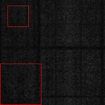
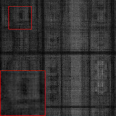
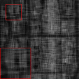
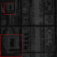
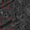
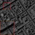
Fig. 3 shows the recovered results of one band and the spectrum profiles of $\mathit{WDC~{}Mall}$ and $\mathit{Pavia~{}City}$ by different methods for SR = 1%. From the visual comparison, our method outperforms other compared methods in preserving image structures and details, e.g., the building in the zoom-in regions of $\mathit{WDC~{}Mall}$. Moreover, NTTNN gives the closest spectrum profiles than those of other compared methods, which demonstrates that the nonlinear transform plays an important role in the spectrum profile recovery.

Table 2: The PSNR, SSIM, and SAM values of the recovered HSIs by different methods for different SRs.

Data Index	methods	SR=1%			SR=5%			SR=10%
		PSNR	SSIM	SAM	PSNR	SSIM	SAM	PSNR	SSIM	SAM
$\mathit{WDC~{}Mall}$	Observed	13.370	0.0083	1.4969	13.549	0.0278	1.3559	13.784	0.0491	1.2556
	TNN	16.499	0.2185	0.5261	28.663	0.8002	0.1743	32.233	0.8974	0.1239
	DCT-TNN	16.540	0.2191	0.5130	29.470	0.8272	0.1525	33.371	0.9199	0.1060
	TTNN	22.646	0.5040	0.2780	32.062	0.9023	0.1105	37.835	0.9721	0.0605
	DTNN	24.587	0.6179	0.2514	32.367	0.9051	0.1196	39.651	0.9788	0.0505
	NTTNN	25.558	0.6749	0.1849	36.402	0.9643	0.0536	43.251	0.9930	0.0219
$\mathit{Pavia~{}City}$	Observed	13.321	0.0076	1.4991	13.500	0.0249	1.3556	13.735	0.0463	1.2547
	TNN	15.643	0.1429	0.5632	28.355	0.8312	0.1879	32.055	0.9119	0.1533
	DCT-TNN	16.464	0.1734	0.4430	30.899	0.9023	0.1273	37.125	0.9733	0.0767
	TTNN	21.477	0.4029	0.1899	32.100	0.9237	0.1099	38.092	0.9787	0.0687
	DTNN	23.190	0.5013	0.1719	31.840	0.9258	0.1006	38.416	0.9819	0.0616
	NTTNN	24.405	0.6587	0.1438	34.498	0.9577	0.0812	41.672	0.9903	0.0468

Observed	TNN	DCT-TNN	TTNN	DTNN	NTTNN	Original

Figure 3: The results of one band and spectrum profiles at one spatial location of HSIs by different methods for SR = 1%. From top to bottom: $\mathit{WDC~{}Mall}$ and $\mathit{Pavia~{}City}$, respectively. From left to right: the observed data, the reconstructed results by TNN, DCT-TNN, TTNN, DTNN, NTTNN, and the original data, respectively.

4.2 Experiments on MSIs Data

In this part, we evaluate different methods on five MSIs from the CAVE database: $\mathit{Balloons}$, $\mathit{Beads}$, $\mathit{Toy}$, $\mathit{Cloth}$, and $\mathit{Feathers}$. All MSIs have been resized to $256\times{256}\times{31}$ in the experiments. The SRs are set to 5%, 10%, and 15%, respectively.

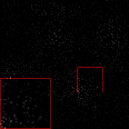
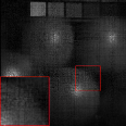
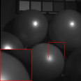
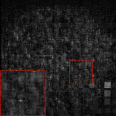
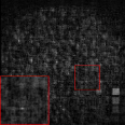
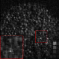
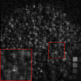
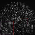
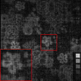
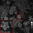
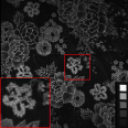
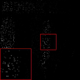
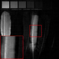
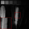
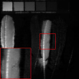
In Table 3, we show the PSNR, SSIM, and SAM values of the recovered MSIs by different methods for different SRs. We can note that NTTNN obtains the highest quality results for different MSIs with different SRs. In addition, Fig. 4 displays the recovered results of one band and spectrum profiles of MSIs by different methods for SR = 5%. From the visual comparison, it is clear that NTTNN performs best in preserving image edges and details, e.g., the symbols in the zoom-in regions of $\mathit{Toy}$. Moreover, we clearly observe that the spectral curves obtained by NTTNN better approximate the original ones than those obtained by the compared methods.

Table 3: The PSNR, SSIM, and SAM values of the recovered MSIs by different methods for different SRs.

Data Index	methods	SR=5%			SR=10%			SR=15%
		PSNR	SSIM	SAM	PSNR	SSIM	SAM	PSNR	SSIM	SAM
$\mathit{Balloons}$	Observed	13.349	0.0959	1.5163	13.762	0.1613	1.2774	14.011	0.1896	1.1934
	TNN	31.642	0.8665	0.1940	36.270	0.9412	0.1230	39.375	0.9681	0.0894
	DCT-TNN	32.639	0.8911	0.1720	37.171	0.9521	0.1099	40.524	0.9758	0.0772
	TTNN	33.641	0.9259	0.1581	37.814	0.9608	0.1005	41.957	0.9830	0.0651
	DTNN	33.418	0.9218	0.1580	37.394	0.9559	0.1145	42.982	0.9831	0.0671
	NTTNN	35.425	0.9387	0.1268	40.458	0.9757	0.0784	43.633	0.9865	0.0600
$\mathit{Beads}$	Observed	14.416	0.1188	1.4032	14.651	0.1548	1.2956	14.898	0.1926	1.2105
	TNN	19.364	0.4086	0.5922	23.508	0.6604	0.4270	26.052	0.7741	0.3381
	DCT-TNN	19.696	0.4272	0.5629	23.434	0.6593	0.4109	26.238	0.7847	0.3181
	TTNN	22.934	0.6789	0.4033	25.786	0.8086	0.3122	28.071	0.8458	0.2662
	DTNN	22.827	0.6950	0.3933	25.659	0.8262	0.2987	30.145	0.9181	0.1895
	NTTNN	23.917	0.7162	0.3784	28.106	0.8659	0.2484	31.327	0.9251	0.1831
$\mathit{Toy}$	Observed	10.631	0.2565	1.3874	10.866	0.2925	1.2821	11.114	0.3271	1.1991
	TNN	28.749	0.8471	0.3287	32.549	0.9197	0.2295	35.453	0.9520	0.1734
	DCT-TNN	28.462	0.8508	0.3054	33.487	0.9396	0.1903	36.599	0.9650	0.1390
	TTNN	29.271	0.8653	0.2986	34.270	0.9435	0.1875	37.801	0.9704	0.1323
	DTNN	29.023	0.8857	0.2998	32.838	0.9306	0.2451	38.470	0.9783	0.1086
	NTTNN	30.636	0.9165	0.2333	35.058	0.9572	0.1659	39.711	0.9798	0.1222
$\mathit{Cloth}$	Observed	11.699	0.0336	1.3939	11.933	0.0578	1.2821	12.181	0.0829	1.1963
	TNN	20.085	0.4275	0.2685	24.889	0.7225	0.1699	27.857	0.8344	0.1285
	DCT-TNN	21.777	0.5225	0.2237	26.227	0.7790	0.1385	29.223	0.8743	0.1026
	TTNN	22.749	0.6077	0.2155	25.458	0.7511	0.1474	28.622	0.8655	0.1070
	DTNN	24.036	0.7139	0.1875	27.883	0.8666	0.1247	31.452	0.9330	0.0874
	NTTNN	25.109	0.7608	0.1464	29.779	0.8971	0.0931	33.345	0.9457	0.0684
$\mathit{Feathers}$	Observed	13.356	0.1907	1.4062	13.590	0.2310	1.3008	13.838	0.2693	1.2162
	TNN	25.029	0.7053	0.3531	31.624	0.8733	0.2063	34.571	0.9235	0.1529
	DCT-TNN	27.842	0.7861	0.2713	32.581	0.8980	0.1697	35.763	0.9428	0.1223
	TTNN	28.650	0.8119	0.2548	33.267	0.9133	0.1539	36.689	0.9546	0.1062
	DTNN	28.164	0.8391	0.3085	33.109	0.9313	0.1725	37.198	0.9635	0.1179
	NTTNN	30.515	0.8801	0.2063	35.581	0.9474	0.1225	39.229	0.9712	0.0883

Observed	TNN	DCT-TNN	TTNN	DTNN	NTTNN	Original

Figure 4: The results of one band and spectrum profiles at one spatial location of MSIs by different methods for SR = 5%. From top to bottom: $\mathit{Balloons}$, $\mathit{Beads}$, $\mathit{Toy}$, $\mathit{Cloth}$, and $\mathit{Feathers}$, respectively. From left to right: the observed data, the reconstructed results by TNN, DCT-TNN, TTNN, DTNN, NTTNN, and the original data, respectively.

4.3 Experiments on Videos Data

In this part, we verify the effectiveness of the proposed NTTNN on three videos: $\mathit{Carphone},\mathit{Hall},$ and $\mathit{News}$. All videos have been resized to $144\times{176}\times{100}$ in the experiments. The SRs are set to 5%, 10%, and 15%, respectively.

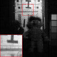
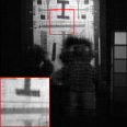
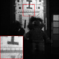
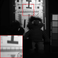
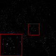
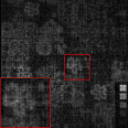
Table 4 shows the quantitative metrics of the recovered videos obtained by different methods for different SRs. We can observe that the proposed NTTNN clearly outperforms the other compared linear transform-based TNN methods for all SRs. For visual comparisons, we show the recovered results of one band and one mode-3 tube of videos by different methods for SR = 5% in Fig. 5. From Fig. 5, we can observe that NTTNN outperforms the compared methods in preserving details and structures, e.g., the dancer in zoom-in regions of $\mathit{News}$. Moreover, NTTNN yields the closest spectral curves in all cases.

Table 4: The PSNR, SSIM, and SAM values of the recovered videos by different methods for different SRs.

Data Index	methods	SR=5%			SR=10%			SR=15%
		PSNR	SSIM	SAM	PSNR	SSIM	SAM	PSNR	SSIM	SAM
$\mathit{Carphone}$	Observed	6.814	0.0143	1.3521	7.048	0.0231	1.2532	7.296	0.0311	1.1758
	TNN	25.122	0.7222	0.1138	27.229	0.7909	0.0942	28.637	0.8309	0.0825
	DCT-TNN	25.516	0.7395	0.1070	27.633	0.8074	0.0881	29.049	0.8459	0.0769
	TTNN	26.597	0.8162	0.0852	28.708	0.8666	0.0724	30.146	0.8932	0.0644
	DTNN	26.941	0.8328	0.0833	29.178	0.8756	0.0694	30.635	0.8983	0.0604
	NTTNN	27.460	0.8355	0.0814	29.614	0.8833	0.0676	31.059	0.9097	0.0588
$\mathit{Hall}$	Observed	4.835	0.0071	1.3516	5.070	0.0123	1.2529	5.319	0.0179	1.1757
	TNN	28.033	0.9010	0.0434	30.868	0.9387	0.0350	32.436	0.9522	0.0309
	DCT-TNN	28.042	0.9034	0.0434	30.842	0.9380	0.0352	32.369	0.9510	0.0311
	TTNN	28.781	0.9163	0.0413	31.283	0.9431	0.0343	32.824	0.9548	0.0303
	DTNN	27.765	0.9040	0.0429	31.722	0.9496	0.0343	33.814	0.9629	0.0295
	NTTNN	30.140	0.9410	0.0352	32.713	0.9595	0.0298	34.261	0.9688	0.0264
$\mathit{News}$	Observed	8.991	0.0207	1.3516	9.227	0.0347	1.2528	9.476	0.0477	1.1756
	TNN	26.715	0.8208	0.1002	29.085	0.8810	0.0814	30.762	0.9119	0.0691
	DCT-TNN	27.069	0.8335	0.0944	29.501	0.8923	0.0756	31.206	0.9222	0.0636
	TTNN	27.674	0.8547	0.0881	30.011	0.9054	0.0705	31.708	0.9319	0.0592
	DTNN	26.277	0.8605	0.0848	29.844	0.9300	0.0646	32.384	0.9479	0.0546
	NTTNN	28.195	0.8896	0.0727	31.028	0.9309	0.0574	32.912	0.9512	0.0479

Observed	TNN	DCT-TNN	TTNN	DTNN	NTTNN	Original

Figure 5: The results of one band and spectral curves at one spatial location of videos by different methods for SR = 5%. From top to bottom: $\mathit{Carphone}$, $\mathit{Hall}$, and $\mathit{News}$, respectively. From left to right: the observed data, the reconstructed results by TNN, DCT-TNN, TTNN, DTNN, NTTNN, and the original data, respectively.

5 Discussion

5.1 Analysis of row number $r$ of $\mathbf{T}$

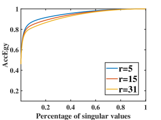
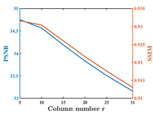
In this subsection, we discuss the influence of row number $r$ of $\mathbf{T}$ on MSI $\mathit{Toy}$ with SR=5%. From the Fig. 6(a), we can observe that the energy of singular values of recovered result of NTTNN with less row number $r$ is more concentrated, which implies that the recovered result of NTTNN with less row number $r$ is more low-rank. Furthermore, Fig. 6(b) plots PSNR and SSIM values of recovered MSIs by NTTNN with different row number $r$ of $\mathbf{T}$. From the Fig. 6(b), we can observed that NTTNN with $r=5$ obtain the best recovered result in terms of PSNR and SSIM values. Therefore, in all experiments, the row number $r$ of $\mathbf{T}$ is selected from {3,4,5,6,7,8,9,10}, which is much less than $n_{3}$.

(a)	(b)

Figure 6: (a) The AccEgy with the corresponding percentage of singular values of recovered results by NTTNN with different row number $r$ of $\mathbf{T}$. (b) The PSNR and SSIM values of NTTNN with different row number $r$ of $\mathbf{T}$.

5.2 The indispensability of $\mathbf{T}$ and $\phi$

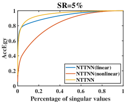
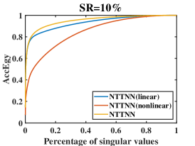
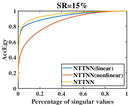
In this part, we analyze the effectiveness of $\mathbf{T}$ and $\phi$ in the proposed nonlinear transform $\psi$ by reserving only $\mathbf{T}$ or $\phi$, which are denoted as NTTNN(linear) and NTTNN(nonlinear), respectively. We conduct the numerical experiment on MSI $\mathit{Toy}$ by NTTNN(linear), NTTNN(nonlinear), and NTTNN with SR 5%, 10%, and 15%, respectively.

Fig. 7 plots curves of the AccEgy with the corresponding percentage of singular values of recovered results by NTTNN(linear), NTTNN(nonlinear), and NTTNN with SR 5%, 10%, and 15%, respectively. We can observe that the linear transform $\mathbf{T}$ and nonlinear transform $\phi$ together contribute to the most concentrate energy of the singular values of recovered results of the proposed NTTNN as compared with the linear transform $\mathbf{T}$ alone and the nonlinear transform $\phi$ alone, i.e., NTTNN(linear) and NTTNN(nonlinear), respectively.

Moreover, Table 5 reports PSNR, SSIM, and SAM values of the recovered MSI $\mathit{Balloons}$ by NTTNN(linear), NTTNN(nonlinear), and NTTNN for different SRs. We can observe that NTTNN outperforms NTTNN(linear) and NTTNN(nonlinear) in terms of PSNR, SSIM, and SAM values due to NTTNN can obtain the most concentrate energy of the singular values of recovered results. Therefore, we suggest the composite nonlinear transform $\psi$ consisting of $\mathbf{T}$ and $\phi$ to obtain a better low-rank approximation of the transformed tensor.

Figure 7: The AccEgy with the corresponding percentage of singular values of recovered results by NTTNN(linear), NTTNN(nonlinear), and NTTNN with SR 5%, 10%, and 15%, respectively.

Table 5: The PSNR, SSIM, and SAM values of the recovered MSI $\mathit{Balloons}$ by NTTNN(linear), NTTNN(nonlinear), and NTTNN for different SRs.

Methods	SR=5%			SR=10%			SR=15%
	PSNR	SSIM	SAM	PSNR	SSIM	SAM	PSNR	SSIM	SAM
Observed			13.349	0.0959	1.5163	13.762	0.1613	1.2774	14.011	0.1896	1.1934
NTTNN(linear)	34.205	0.9322	0.1476	37.890	0.9643	0.1115	39.870	0.9746	0.0958
NTTNN(nonlinear)	19.823	0.4974	0.3798	24.280	0.6990	0.2521	27.477	0.8090	0.1898
NTTNN	35.425	0.9387	0.1268	40.458	0.9757	0.0784	43.633	0.9865	0.0600

5.3 Effectiveness of nonlinear transform

In this subsection, we further verify the effectiveness of nonlinear transform in the proposed framework. Specifically, we compare the performance of NTTNN without nonlinear function $\phi$ (denoted as NTTNN(linear)) and NTTNN with different nonlinear transforms, i.e., Sigmoid function [44], Softplus function [45], and Hyperbolic tangent (Tanh) function [44].

Table 6 reports the PSNR, SSIM, and SAM values of the recovered HSI $\mathit{WDC~{}Mall}$ by NTTNN with different nonlinear function for different SRs. We can observe that NTTNN(Tanh) obtains the best recovered results for SR 5% and 10%, while NTTNN(Sigmoid) obtains the best recovered results for challenging case SR 1%. Additionally, the performance of NTTNN with different nonlinear functions compared with NTTNN(linear) is improved, which demonstrates the nonlinear function play an important role in our NTTNN framework.

Table 6: The PSNR, SSIM, and SAM values of the recovered HSI $\mathit{WDC~{}Mall}$ by NTTNN with different nonlinear functions for different SRs.

Methods	SR=1%			SR=5%			SR=10%
	PSNR	SSIM	SAM	PSNR	SSIM	SAM	PSNR	SSIM	SAM
Observed			13.370	0.0083	1.4969	13.549	0.0278	1.3559	13.784	0.0491	1.2556
NTTNN(linear)	24.863	0.6188	0.1928	33.882	0.9337	0.0787	38.635	0.9766	0.0474
NTTNN(Sigmoid)	26.523	0.7142	0.1723	34.287	0.9414	0.0663	41.462	0.9885	0.0260
NTTNN(Softplus)	25.987	0.6866	0.1881	34.713	0.9465	0.0651	42.159	0.9904	0.0247
TTNN(Tanh)	25.558	0.6749	0.1849	36.402	0.9643	0.0536	43.251	0.9930	0.0219

5.4 Comparison of different initialization

In this subsection, we discuss the performance of NTTNN with different initialization of $\mathcal{X}$. We consider initializing $\mathcal{X}^{0}$ by the following: the observed tensor, the result of TNN method, and the linear interpolation of $\mathcal{X}^{0}$, which denote as NTTNN(Observed), NTTNN(TNN), and NTTNN(Interpolation), respectively.

Table 7 reports the PSNR, SSIM, and SAM values of the recovered HSI $\mathit{WDC~{}Mall}$ by NTTNN(Observed), NTTNN(TNN), and NTTNN(Interpolation) for different SRs. We can observe that NTTNN(Interpolation) and NTTNN(TNN) outperform NTTNN(Observed) for all SRs, which demonstrates using good and low computational cost initialization can improve the performance of NTTNN. Additionally, NTTNN(Interpolation) outperforms NTTNN(TNN) for extremely low SRs 1% and 5%, and both of them obtain good performance for relatively high SR 10%. The reason behind this phenomenon is the interpolation method outperforms the TNN method for extremely low SRs. Therefore, throughout all the experiments in this paper, we employ good and low computational cost linear interpolation strategy to fill in the missing pixels and obtain $\mathcal{X}^{0}$ for TTNN, DTNN, and our method.

Table 7: The PSNR, SSIM, and SAM values of the recovered HSI $\mathit{WDC~{}Mall}$ by NTTNN with different initialization for different SRs.

methods	SR=1%			SR=5%			SR=10%
	PSNR	SSIM	SAM	PSNR	SSIM	SAM	PSNR	SSIM	SAM
NTTNN(Observed)			21.391	0.4825	0.3212	33.980	0.9347	0.0758	40.193	0.9802	0.0510
NTTNN(TNN)	22.651	0.5544	0.2283	35.863	0.9544	0.0554	43.969	0.9919	0.0256
NTTNN(Interpolation)	25.558	0.6749	0.1849	36.402	0.9643	0.0536	43.251	0.9930	0.0219

5.5 Numerical convergence

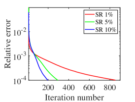
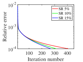
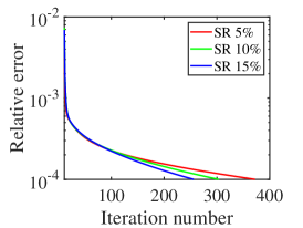
In this subsection, we evaluate the numerical convergence of the PAM-based algorithm for the proposed method to validate the theoretical convergence. Taking the HSI $\mathit{WDC~{}Mall}$, MSI $\mathit{Balloons}$, and video $\mathit{Carphone}$ for different SRs as examples, Fig. 8 displays the relative change curves of the proposed PAM-based algorithm. We can clearly observe that the relative error decreases as the number of iterations increase, demonstrating the numerical convergence of the proposed PAM-based algorithm.

(a)	(b)	(c)

Figure 8: Curves of relative errors versus iterations. (a) HSI $\mathit{WDC~{}Mall}$. (b) MSI $\mathit{Balloons}$. (c) Video $\mathit{Carphone}$.

6 Conclusion

In this paper, we proposed the nonlinear transform for the underlying tensor and developed the corresponding nonlinear transform-based TNN (NTTNN). More concretely, the proposed nonlinear transform is a composite transform consisting of the linear semi-orthogonal transform along the third mode and the element-wise nonlinear transform on frontal slices of the tensor under the linear semi-orthogonal transform, which are indispensable and complementary in the composite transform to fully exploit the underlying low-rankness. The proposed NTTNN could enhance the low-rank approximation of the underlying tensor and can be regarded as a unified transform-based TNN family including many classic transform-based TNN methods. Moreover, based on the suggested low-rank metric, i.e., NTTNN, we proposed the corresponding LRTC model and developed an efficient PAM-based algorithm. Theoretically, we proved that the sequence generated by the proposed method is bounded and converges to a critical point. Massive experimental results on different types of multi-dimensional images show that NTTNN reconstructs better results compared to the state-of-the-art linear transform-based TNN methods quantitatively and visually.

References

- [1] X. Zhao, M. Bai, and M. K. Ng, “Nonconvex optimization for robust tensor completion from grossly sparse observations,” J. Sci. Comput., vol. 85, p. 46, 2020.
- [2] W. He, Q. Yao, C. Li, N. Yokoya, Q. Zhao, H. Zhang, and L. Zhang, “Non-local meets global: An integrated paradigm for hyperspectral image restoration,” IEEE Trans. Pattern Anal. Mach. Intell., pp. 1–1, 2020, doi:10.1109/TPAMI.2020.3027563.
- [3] M. Ding, T.-Z. Huang, T.-Y. Ji, X.-L. Zhao, and J.-H. Yang, “Low-rank tensor completion using matrix factorization based on tensor train rank and total variation,” J. Sci. Comput., vol. 81, pp. 941–964, 2019.
- [4] X. Zhang and M. K. Ng, “Low rank tensor completion with Poisson observations,” IEEE Trans. Pattern Anal. Mach. Intell., doi:10.1109/TPAMI.2021.3059299.
- [5] C. Shi, Z. Huang, and T. Wan, Li Xiong, “Low-rank tensor completion based on log-Det rank approximation and matrix factorization,” J. Sci. Comput., vol. 80, pp. 1888–1912, 2019.
- [6] A. Buccini and L. Reichel, “An regularization method for large discrete ill-posed problems,” J. Sci. Comput., vol. 78, pp. 1526–1549, 2019.
- [7] M. Che, Y. Wei, and H. Yan, “An efficient randomized algorithm for computing the approximate Tucker decomposition,” J. Sci. Comput., vol. 88, 2021, doi:10.1007/s10915-021-01545-5.
- [8] J.-F. Li, W. Li, S.-W. Vong, Q.-L. Luo, and M. Xiao, “A riemannian optimization approach for solving the generalized eigenvalue problem for nonsquare matrix pencils,” J. Sci. Comput., vol. 82, 2020, doi:10.1007/s10915-020-01173-5.
- [9] Y. Wang, W. Yin, and J. Zeng, “Global convergence of ADMM in nonconvex nonsmooth optimization,” J. Sci. Comput., vol. 78, pp. 29–63, 2019.
- [10] F. L. Hitchcock, “The expression of a tensor or a polyadic as a sum of products,” Studies in Appl. Math., vol. 6, no. 1-4, pp. 164–189, 1927.
- [11] Q. Zhao, L. Zhang, and A. Cichocki, “Bayesian CP factorization of incomplete tensors with automatic rank determination,” IEEE Trans. Pattern Anal. Mach. Intell., vol. 37, no. 9, pp. 1751–1763, 2015.
- [12] J. Xue, Y. Zhao, S. Huang, W. Liao, J. C.-W. Chan, and S. G. Kong, “Multilayer sparsity-based tensor decomposition for low-rank tensor completion,” IEEE Trans. Neural Netws. Learn. Syst., pp. 1–15, 2021, doi:10.1109/TNNLS.2021.3083931.
- [13] C. J. Hillar and L.-H. Lim, “Most tensor problems are NP-hard,” J. ACM, vol. 60, no. 6, 2013.
- [14] J. Liu, P. Musialski, P. Wonka, and J. Ye, “Tensor completion for estimating missing values in visual data,” IEEE Trans. Pattern Anal. Mach. Intell., vol. 35, no. 1, pp. 208–220, 2012.
- [15] T.-Y. Ji, T.-Z. Huang, X.-L. Zhao, T.-H. Ma, and L.-J. Deng, “A non-convex tensor rank approximation for tensor completion,” Appl. Math. Model., vol. 48, pp. 410–422, 2017.
- [16] W. Cao, Y. Wang, C. Yang, X. Chang, Z. Han, and Z. Xu, “Folded-concave penalization approaches to tensor completion,” Neurocomput., vol. 152, pp. 261–273, 2015.
- [17] I. V. Oseledets, “Tensor-train decomposition,” SIAM J. Sci. Comput., vol. 33, no. 5, pp. 2295–2317, 2011.
- [18] Q. Zhao, G. Zhou, S. Xie, L. Zhang, and A. Cichocki, “Tensor ring decomposition,” arXiv preprint arXiv:1606.05535, 2016.
- [19] Y.-B. Zheng, T.-Z. Huang, X.-L. Zhao, Q. Zhao, and T.-X. Jiang, “Fully-connected tensor network decomposition and its application to higher-order tensor completion,” In Proceedings of AAAI Conf. Artifi. Intell., vol. 35, pp. 11 071–11 078, 2021.
- [20] J. Bengua, H. Phien, T. Hoang, and M. do, “Efficient tensor completion for color image and video recovery: Low-rank tensor train,” IEEE Trans. Image Process., vol. 26, pp. 2466 – 2479, 2017.
- [21] L. Yuan, C. Li, D. Mandic, J. Cao, and Q. Zhao, “Tensor ring decomposition with rank minimization on latent space: An efficient approach for tensor completion,” In Proceedings of AAAI Conf. Artifi. Intell., vol. 33, pp. 9151–9158, 2019.
- [22] M. Kilmer and C. Martin, “Factorization strategies for third-order tensors,” Linear Algeb. Appli., vol. 435, no. 3, pp. 641–658, 2011.
- [23] Z. Zhang, G. Ely, S. Aeron, N. Hao, and M. Kilmer, “Novel methods for multilinear data completion and de-noising based on tensor-svd,” Conference on CVPR, pp. 3842–3849, 2014.
- [24] C. Lu, X. Peng, and Y. Wei, “Low-rank tensor completion with a new tensor nuclear norm induced by invertible linear transforms,” Conference on CVPR, pp. 5989–5997, 2019.
- [25] W.-H. Xu, X.-L. Zhao, and M. K. Ng, “A fast algorithm for cosine transform based tensor singular value decomposition,” arXiv:1902.03070, 2019.
- [26] E. Kernfeld, M. Kilmer, and S. Aeron, “Tensor-tensor products with invertible linear transforms,” Linear Algeb. Appli., vol. 485, pp. 545–570, 2015.
- [27] T. Jiang, M. K. Ng, X. Zhao, and T. Huang, “Framelet representation of tensor nuclear norm for third-order tensor completion,” IEEE Trans. Image Process., vol. 29, pp. 7233–7244, 2020.
- [28] G. Song, M. Ng, and X. Zhang, “Robust tensor completion using transformed tensor singular value decomposition,” Numer. Linear Algeb. Appl., vol. 27, p. 2299, 2020.
- [29] H. Kong, C. Lu, and Z. Lin, “Tensor Q-rank: New data dependent tensor rank,” Mach. Learn., vol. 110, pp. 1867–1900, 2021.
- [30] T.-X. Jiang, X.-L. Zhao, H. Zhang, and M. K. Ng, “Dictionary learning with low-rank coding coefficients for tensor completion,” IEEE Trans. Neural Netws. Learn. Syst., 2021, doi:10.1109/TNNLS.2021.3104837.
- [31] T. G. Kolda and B. W. Bader, “Tensor decompositions and applications,” SIAM Review, vol. 51, no. 3, pp. 455–500, 2009.
- [32] J. Wang, Y. Chen, R. Chakraborty, and S. X. Yu, “Orthogonal convolutional neural networks,” Proceedings of the Conference on CVPR, pp. 11 505–11 515, 2020.
- [33] K. Jia, S. Li, Y. Wen, T. Liu, and D. Tao, “Orthogonal deep neural networks,” IEEE Trans. Pattern Anal. Mach. Intell., 2019, doi:10.1109/TPAMI.2019.2948352.
- [34] N. Bansal, X. Chen, and Z. Wang, “Can we gain more from orthogonality regularizations in training deep CNNs?” arXiv preprint arXiv:1810.09102, 2018.
- [35] D. Krishnan and R. Fergus, “Fast image deconvolution using hyper-laplacian priors,” Advances in Neural Inform. Process. Syst., pp. 1033–1041, 2009.
- [36] Z. Li, S. Ding, W. Chen, Z. Yang, and S. Xie, “Proximal alternating minimization for analysis dictionary learning and convergence analysis,” IEEE Trans. Emerg. Topics in Comput. Intell., vol. 2, no. 6, pp. 439–449, 2018.
- [37] J.-F. Cai, E. J. Candès, and Z. Shen, “A singular value thresholding algorithm for matrix completion,” SIAM J. Optim., vol. 20, no. 4, pp. 1956–1982, 2010.
- [38] H. Attouch, J. Bolte, and B. Svaiter, “Convergence of descent methods for semi-algebraic and tame problems: Proximal algorithms, forward-backward splitting, and regularized Gauss-Seidel methods,” Math. Program., vol. 137, pp. 91–129, 2013.
- [39] J. Bolte, S. Sabach, and T. M, “Proximal alternating linearized minimization for nonconvex and nonsmooth problems,” Math. Program., vol. 46, 2014.
- [40] J. Zeng, T. T.-K. Lau, S. Lin, and Y. Yao, “Global convergence of block coordinate descent in deep learning,” Proceedings of the 36th Inter. Conf. Mach. Learn., vol. 97, pp. 7313–7323, 2019.
- [41] N. Yair and T. Michaeli, “Multi-scale weighted nuclear norm image restoration,” Conference on CVPR, pp. 3165–3174, 2018.
- [42] Z. Wang, A. C. Bovik, H. R. Sheikh, and E. P. Simoncelli, “Image quality assessment: from error visibility to structural similarity,” IEEE Trans. Image Process., vol. 13, no. 4, pp. 600–612, 2004.
- [43] B. R. Shivakumar and S. V. Rajashekararadhya, “Performance evaluation of spectral angle mapper and spectral correlation mapper classifiers over multiple remote sensor data,” Proceeding of 2017 Second International Conference on Electrical, Computer and Communication Technologies, pp. 1–6, 2017.
- [44] S. Haykin, “Neural networks : a comprehensive foundation”. Prentice Hall, July 1998.
- [45] V. Nair and G. E. Hinton, “Rectified linear units improve restricted boltzmann machines,” Proceedings of the 27th International Conference on International Conference on Mach. Learn., pp. 807–814, 2010.