S-Cyc: A Learning Rate Schedule for Iterative Pruning of ReLU-based Networks

Abstract

We explore a new perspective on adapting the learning rate (LR) schedule to improve the performance of the ReLU-based network as it is iteratively pruned. Our work and contribution consist of four parts: (i) We find that, as the ReLU-based network is iteratively pruned, the distribution of weight gradients tends to become narrower. This leads to the finding that as the network becomes more sparse, a larger value of LR should be used to train the pruned network. (ii) Motivated by this finding, we propose a novel LR schedule, called S-Cyclical (S-Cyc) which adapts the conventional cyclical LR schedule by gradually increasing the LR upper bound (max_lr) in an S-shape as the network is iteratively pruned. We highlight that S-Cyc is a method agnostic LR schedule that applies to many iterative pruning methods. (iii) We evaluate the performance of the proposed S-Cyc and compare it to four LR schedule benchmarks. Our experimental results on three state-of-the-art networks (e.g., VGG-19, ResNet-20, ResNet-50) and two popular datasets (e.g., CIFAR-10, ImageNet-200) demonstrate that S-Cyc consistently outperforms the best performing benchmark with an improvement of 2.1% - 3.4%, without substantial increase in complexity. (iv) We evaluate S-Cyc against an oracle and show that S-Cyc achieves comparable performance to the oracle, which carefully tunes max_lr via grid search.

1 Introduction

Network pruning is a process of removing weights, filters or neurons from neural networks (LeCun, Denker, and Solla 1990; Han et al. 2015; Li et al. 2017). Several state-of-the-art pruning methods (Renda, Frankle, and Carbin 2020; Frankle and Carbin 2019; Frankle et al. 2020) have demonstrated that a large amount of parameters can be removed without sacrificing accuracy. This greatly reduces the resource demand of neural networks, such as storage requirements and energy consumption (Han et al. 2015; Li et al. 2017).

The inspiring performance of pruning methods hinges on a key factor - Learning Rate (LR) - as mentioned in prior works (Renda, Frankle, and Carbin 2020; Frankle and Carbin 2019). Specifically, Frankle and Carbin (2019) propose the concept of the Lottery Ticket Hypothesis and demonstrate that the winning tickets (i.e., the pruned subnetwork that can train in isolation to full accuracy) cannot be found without applying a LR warmup schedule. In a follow-up work, Renda, Frankle, and Carbin (2020) propose LR rewinding which rewinds the LR schedule to its initial state during iterative pruning and demonstrate that it can outperform standard fine-tuning. Overall, these two works suggest that LR plays an important role in network pruning.

In this paper, we take the investigation one step further and explore a new perspective on adapting the LR schedule to improve the iterative pruning performance of the ReLU-based network. Our contributions are as follows.

1. Via extensive experiments on various networks, datasets and pruning methods, we find that, as the ReLU-based network is iteratively pruned, the distribution of weight gradients tends to become narrower, suggesting that a larger value of LR should be used for pruning.

2. We propose a novel LR schedule called the S-Cyclical (S-Cyc) which adapts the conventional cyclical LR (Smith 2017) by gradually increasing the LR upper bound (max_lr) in an S-shape as the ReLU-based neural network is iteratively pruned.

3. We compare the performance of S-Cyc to four LR schedule benchmarks on three state-of-the-art networks (e.g., VGG-19 (Simonyan and Zisserman 2014), ResNet-20, ResNet-50 (He et al. 2016)) and two popular datasets (e.g., CIFAR-10 (Krizhevsky et al. 2009), ImageNet-200 (Le and Yang 2015)). Our experimental results demonstrate S-Cyc consistently outperforms the best performing benchmark with an improvement of 2.1% - 3.4%.

4. We investigate the trajectory of max_lr at each pruning cycle. Our results demonstrate that the value of max_lr estimated by S-Cyc is very competitive, i.e., it can achieve comparable performance to a greedy oracle which carefully tunes max_lr via grid search.

2 Network Pruning and Learning Rate

In Section 2.1, we first review prior work on network pruning. Next, in Section 2.2, we highlight the important role of LR in network pruning and position our work accordingly.

2.1 Prior Works on Network Pruning

Network pruning is an established idea dating back to 1990 (LeCun, Denker, and Solla 1990). The motivation is that neural networks tend to be overparameterized and redundant weights can be removed with a negligible loss in accuracy (Arora, Cohen, and Hazan 2018; Allen-Zhu, Li, and Song 2019; Denil et al. 2013). Given a trained network, one pruning cycle consists of three steps as follows.

1. Prune the network according to certain heuristics.

2. Freeze pruned parameters as zero.

3. Retrain the pruned network to recover the accuracy.

Repeating the pruning cycle multiple times until the target sparsity or accuracy is met is known as iterative pruning. Doing so often results in better performance than one-shot pruning (i.e., perform only one pruning cycle) (Han et al. 2015; Frankle and Carbin 2019; Li et al. 2017). There are two types of network pruning - unstructured and structured - which will be discussed in detail below.

Unstructured Pruning: Unstructured pruning removes individual weights according to certain heuristics such as magnitude (Han et al. 2015; Frankle and Carbin 2019) or gradient (Hassibi and Stork 1993; LeCun, Denker, and Solla 1990; Lee et al. 2018; Xiao, Wang, and Rajasekaran 2019; Theis et al. 2018). Examples are (LeCun, Denker, and Solla 1990), which performs pruning based on the Hessian Matrix, and (Theis et al. 2018), which uses Fisher information to approximate the Hessian Matrix. Similarly, Han et al. (2015) remove weights with the smallest magnitude and this approach was further incorporated with the three-stage iterative pruning pipeline in (Han, Mao, and Dally 2015).

Structured Pruning: Structured pruning involves pruning weights in groups, neurons, channels or filters (Yang et al. 2019; Molchanov et al. 2017, 2019; Luo, Wu, and Lin 2017; Yu et al. 2018; Tan and Motani 2020; Wang et al. 2020b; Lin et al. 2020). Examples are (Hu et al. 2016), which removes neurons with high average zero output ratio, and (Li et al. 2017), which prunes neurons with the lowest absolute summation values of incoming weights. More recently, Yu et al. (2018) propose the neuron importance score propagation algorithm to evaluate the importance of network structures. Molchanov et al. (2019) use Taylor expansions to approximate a filter’s contribution to final loss and Wang et al. (2020) optimize the neural network architecture, pruning policy, and quantization policy in a joint manner.

Other Works: In addition to works mentioned above, several other works also share some deeper insights in network pruning (Liu et al. 2019; Zhu and Gupta 2018; Liu, Simonyan, and Yang 2018; Wang et al. 2020c). For example, Liu, Simonyan, and Yang (2018) demonstrate that training-from-scratch on the right sparse architecture yields better results than pruning from pre-trained models. Similarly, Wang et al. (2020) suggest that the fully-trained network could reduce the search space for the pruned structure. More recently, Yeom et al. (2021) evaluate the importance of the network structure using their relevance computed via the concepts of explainable AI, connecting interpretability to model compression. Luo and Wu (2020) address the issue of pruning residual connections with limited data and Ye et al. (2020) theoretically prove the existence of small subnetworks with lower loss than the unpruned network. One milestone paper (Frankle and Carbin 2019) points out that reinitializing with the original parameters plays an important role in network pruning and helps to further prune the network with negligible loss in accuracy. Some follow-on works (Zhou et al. 2019; Frankle et al. 2019; Renda, Frankle, and Carbin 2020; Malach et al. 2020) investigate this phenomenon more precisely and apply this method in other fields (e.g., transfer learning (Mehta 2019), reinforcement learning and natural language processing (Yu et al. 2019)).

2.2 The Important Role of LR and Our Work

Several recent works (Renda, Frankle, and Carbin 2020; Frankle and Carbin 2019) have noticed the important role of LR in network pruning. For example, Frankle and Carbin (2019) demonstrate that training VGG-19 (Simonyan and Zisserman 2014) with a LR warmup schedule (i.e., increase LR to 1e-1 first and decrease it to 1e-3) and a constant LR of 1e-2 results in comparable accuracy for the unpruned network. However, as the network is iteratively pruned, the LR warmup schedule leads to a much higher accuracy (see Fig.7 in (Frankle and Carbin 2019)). One follow-up work (Renda, Frankle, and Carbin 2020) further investigates this phenomenon and proposes a retraining technique called LR rewinding. They demonstrate that LR rewinding can always outperform the standard retraining technique called fine-tuning (Han et al. 2015). The difference is that fine-tuning trains the unpruned network with a LR warmup schedule, and then it retrains the pruned network with a constant LR (i.e., the final LR of the LR warmup schedule) in subsequent pruning cycles (Liu et al. 2019). LR rewinding retrains the pruned network by rewinding the LR warmup schedule to its initial state, which is equivalent to using the same LR warmup schedule for subsequent pruning cycles. As an example, they train the ResNet-50 (He et al. 2016) with a LR warmup schedule (i.e., increase LR to 0.4 and decrease it to 4e-4). The performance of LR rewinding and fine-tuning are comparable for the unpruned network. However, as the network is iteratively pruned, LR rewinding leads to a much higher accuracy (see Figs.1 & 2 in (Renda, Frankle, and Carbin 2020)). Overall, both of these two works suggest that LR plays an important role in network pruning.

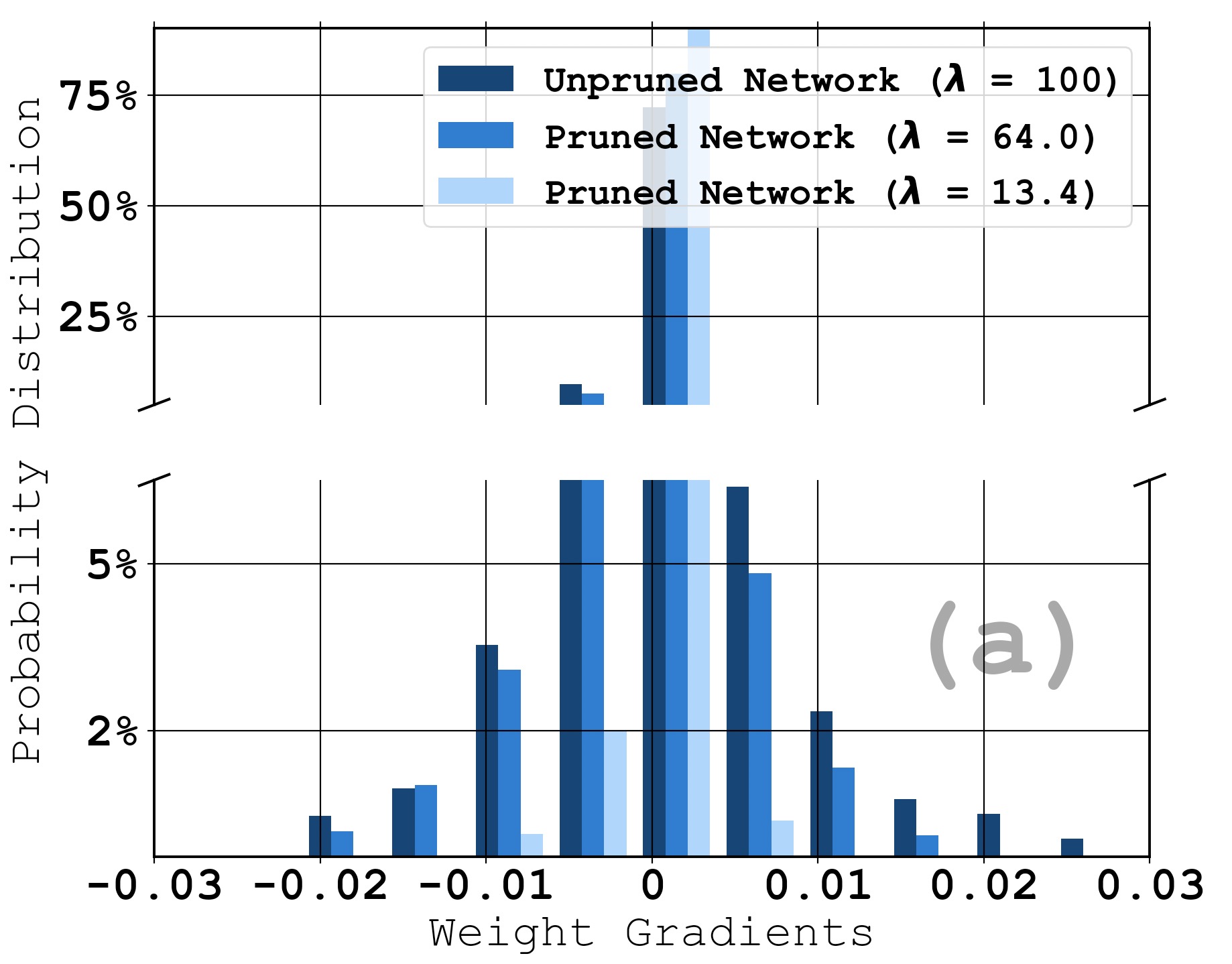
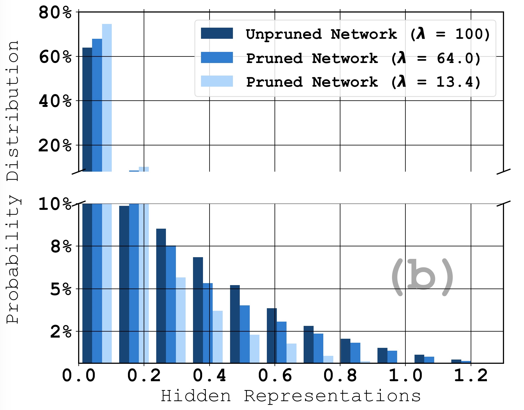
Figure 1: (a) The distribution of all weight gradients when iteratively pruning a fully connected ReLU-based network using global magnitude pruning method (Han et al. 2015), where $\lambda$ is the percent of weights remaining. (b) The corresponding distribution of hidden representations (i.e., post-activation outputs of all hidden layers). Please note that there is a line breaker in the vertical axis. We note that this finding generalizes to other networks, datasets and pruning methods (see Section 3.3).

Our work takes the investigation one step further and explores a new perspective on adapting the LR schedule to improve the iterative pruning performance of the ReLU-based network. The proposed LR schedule is method agnostic and applies to many iterative pruning methods. We chose to focus on iterative pruning of ReLU-based networks for two reasons: (i) Iterative pruning tends to provide better pruning performance than one-shot pruning as reported in the literature (Frankle and Carbin 2019; Renda, Frankle, and Carbin 2020). (ii) ReLU has been widely used in many state-of-the-art neural networks (e.g., ResNet, VGG). Those networks have achieved outstanding performance in various tasks (He et al. 2016; Simonyan and Zisserman 2014).

3 A New Insight on Network Pruning

In this section, we first provide a new insight in network pruning using empirical results in Section 3.1. In Section 3.2, we provide a possible explanation for the new insight. In Section 3.3, we highlight that this new insight can be generalized to other networks, datasets and pruning methods.

3.1 An Experiment and a New Insight

We first design a fully connected ReLU-based neural network with three hidden layers of 256 neurons each. We train the neural network using a randomly selected subset (80%) from the Fashion-MNIST dataset via SGD (Ruder 2016) (LR = 1e-3, momentum = 0.9) with a batch size of 64 for 500 epochs. We note that all weights are initialized using He Initialization (He et al. 2015) and all hyper-parameters are tuned for performance via grid search (e.g., LR from 1e-4 to 1e-2). We apply the global magnitude pruning (Han et al. 2015) (i.e., removing weights with the smallest magnitudes anywhere in the network) with a pruning rate of 0.2 (i.e., prune 20% of the remaining parameters) to iteratively prune the network for 10 pruning cycles and plot the distribution of all weight gradients at the end of training in Fig. 1 (a), where $\lambda$ is the percent of weights remaining. There are 10 visible bins estimated by the the Sturges Rule and the edge values rang from -0.021 to 0.027 with a bin width of 0.004.

In Fig.1 (a), we observe that the distribution of weight gradients tends to become less heavy-tailed as the network is iteratively pruned. For example, the unpruned network ($\lambda$ = 100) has more than 6% of weight gradients with values greater than 0.009 (rightmost 4 bars) or less than -0.011 (leftmost 2 bars), while the pruned network ($\lambda=13.4$) has less than 1% of weight gradients falling into those regions.

During the training of network, the weight update of $w_{i}$ is

$$w_{i}\leftarrow w_{i}+\alpha\frac{\partial\mathcal{L}}{\partial w_{i}},$$ (1)

where $\alpha$ is the LR and $\mathcal{L}$ is the loss function.

New Insight: Assume that $\alpha$ is well-tuned to ensure the weight update (i.e., $\alpha\frac{\partial\mathcal{L}}{\partial w_{i}}$) is sufficiently large to prevent the network from getting stuck in local optimal points (Bengio 2012; Goodfellow, Bengio, and Courville 2016). In Fig. 1 (a), the magnitude of weight gradients (i.e., $\frac{\partial\mathcal{L}}{\partial w_{i}}$) tends to decrease as the network is iteratively pruned. To preserve the same weight updating size and effect as before, a larger value of LR ($\alpha$) should be used to train the pruned network.

3.2 Result Analysis

We now provide a possible explanation for the change in the distribution of weight gradients. We assume each $x_{i}w_{i}$ (i.e., the scalar neuron input $\times$ its associated scalar weight) is an i.i.d. random variable. Then, the variance of the neuron’s pre-activation output ($\sum_{i=1}^{n}x_{i}w_{i}$, $n$ is the number of inputs) will be $\sum_{i=1}^{n}\text{Var}(x_{i}w_{i})$. Pruning the network is equivalent to reducing the number of inputs from $n$ to $n-k$, resulting in a smaller variance of $\sum_{i=1}^{n-k}\text{Var}(x_{i}w_{i})$. Hence, the distribution of the pre-activation output after pruning is narrower. Since ReLU returns its raw input if the input is positive, the distribution of hidden representations (i.e., post-activation outputs) becomes narrower as well. This can be verified from Fig. 1 (b), where we plot the distribution of hidden representation (i.e., post-activation output of all hidden layers) from the experiment in Section 3.1. We note that the weight gradient $\frac{\partial\mathcal{L}}{\partial w_{i}}$ is proportional to the hidden representation $x_{i}$ that associates with $w_{i}$ (i.e., $\frac{\partial\mathcal{L}}{\partial w_{i}}\propto x_{i}$). Therefore, as the network is iteratively pruned, the distribution of hidden representations tends to become narrower (see Fig. 1 (b)), leading to a narrower distribution of weight gradients (see Fig. 1 (a)). As a result, a larger value of LR should be used to ensure the weight update is sufficiently large.

Algorithm 1 Algorithm of the Proposed S-Cyc

1:(1) lower bound $\epsilon$, (2) upper bound $\delta+\epsilon$, (3) pruning rate p, (4) number of pruning cycles L, (5) number of training epochs t, (6) S-shape control term $\beta$, (7) delay term q.

2:for $\texttt{m}=0$ to L do

3:     if $\texttt{m}\leq\texttt{q}$ then $\texttt{max\_lr}=\epsilon$

4:     else $\texttt{max\_lr}=\frac{\delta}{1+(\frac{\gamma}{1-\gamma})^{-\beta}}+\epsilon$, where $\gamma=1-(1-\texttt{p})^{m-\texttt{q}}$      

5:     for $\texttt{i}=0$ to t do

6:         linearly warmup learning rate to max_lr

7:         then drop it multiple times at certain epochs      

Figure 2: Illustration of the Proposed S-Cyc Learning Rate Schedule (left) and its detailed algorithm (right).

3.3 More Experimental Results

Effect of Batch Normalization: Batch Normalization (BN) (Ioffe and Szegedy 2015) is a popular technique to reformat the distribution of hidden representations, so as to address the issue of internal covariate shift. To examine the effect of BN , we apply BN ($\mu$ = 0, $\sigma^{2}$ = 1) to each hidden layer (before ReLU) and re-plot the distribution of hidden representations and weight gradients (see Fig. 3 in the Appendix). We note that BN slightly reduces the change in the distribution of hidden representations and weight gradients as the network is iteratively pruned, but the trend still largely mirrors those in Fig. 1 (a) & (b). As an example, the unpruned network ($\lambda$ = 100) has about 3% of weight gradients with values greater than 0.03 (rightmost bar) or less than -0.024 (leftmost bar), while the pruned network ($\lambda$ = 13.4) has less than 1% of weight gradients falling into those regions.

Other Pruning Methods, Datasets and Networks: In addition to the global magnitude pruning, two unstructured pruning methods (i.e., layer magnitude, global gradient) suggested by (Blalock et al. 2020) and one structured pruning method (L1 norm pruning) (Li et al. 2017) are examined as well. Those methods are used to iteratively prune AlexNet (Krizhevsky and Hinton 2010), ResNet-20 and VGG-16 on the CIFAR-10 dataset. The network parameters are summarized in Table. 4 in the Appendix. The results shown in Figs. 4 - 6 in the Appendix largely mirror those in Figs. 1 as well.

4 A New Learning Rate Schedule

In Section 4.1, we review existing works on LR and shortlist four benchmarks for comparison. In Section 4.2, we introduce the idea of S-Cyc and highlight the difference with existing works. In Section 4.3, we detail the S-Cyc algorithm.

4.1 LR Schedule Benchmarks

Learning rate is the most important hyper-parameter in training networks (Goodfellow, Bengio, and Courville 2016). The LR schedule is to adjust LR during training by a pre-defined schedule. Common LR schedules are

1. LR Decay starts with a large initial LR and decays it by a certain factor after a pre-defined number of epochs. Several works (You et al. 2019; Ge et al. 2019; An et al. 2017) have demonstrated that decaying LR helps the network converge better and avoids undesired oscillations.

2. LR Warmup is to increase the LR to a large value over certain epochs and then decreases the LR by a certain factor. It is a popular schedule used by many practitioners for transfer learning (He et al. 2019) and network pruning (Frankle and Carbin 2019; Frankle et al. 2020).

3. Cyclical LR (Smith 2017) is to vary the LR cyclically between a pre-defined lower bound and upper bound. LR Warmup can be considered as a special form of the Cyclical LR. The difference is that the LR Warmup does only one up-and-down cycle while the Cyclical LR repeats the up-and-down cycle multiple times.

All of the three LR schedules and constant LR will be used as benchmarks for comparison. For the proposed S-Cyc, we evaluate its performance using SGD with momentum = 0.9 and a weight decay of 1e-4 (same as (Renda, Frankle, and Carbin 2020; Frankle and Carbin 2019)).

We note that, in addition to LR schedules which vary LR by a pre-defined schedule, adaptive learning rate optimizers such as AdaDelta (Zeiler 2012), Adam (Kingma and Ba 2014) and RMSProp (Tieleman and Hinton 2012) provide heuristic based approaches to adaptively vary the step size of weight update based on observed statistics of the past gradients. All of them are sophisticated optimization algorithms and much work (Gandikota et al. 2021; Jentzen et al. 2021) has been done to investigate their behaviours and mechanisms. The effect of those adaptive LR optimizers on the proposed S-Cyc will be discussed in Section 6.

4.2 S-Cyclical Learning Rate Schedule

In Sections 3.2, we find that as the ReLU-based network is iteratively pruned, the distribution of weight gradients becomes narrower, and a larger value of LR should be used. This motivates us to propose S-Cyc LR schedule for iterative pruning of ReLU-based networks. As illustrated in Fig. 2, the main idea of the proposed S-Cyc is to apply the LR warmup schedule for every pruning cycle, with a gradual increase of the LR upper bound (i.e., max_lr) in an S-shape as the network is iteratively pruned. The LR warmup schedule for one pruning cycle first increases the value of LR to max_lr, maintains its value, then decreases it sharply. This LR warmup schedule is meant to be flexible and can change depending on different neural networks and datasets.

The proposed S-Cyc consists of four phases as follows:

1. In the phase of No Growth, we do not increase max_lr until the pruning cycle q (see Fig. 2), where q is a tunable parameter. It is because the unpruned network usually contains a certain amount of weights with zero magnitude. Those parameters are likely to be pruned at the first few pruning cycles, and removing such weights has negligible effect on the distribution of weight gradients. For example, in Fig. 4 in the Appendix, we compare the pruned network ($\lambda$ = 80) to the unpruned network and observe very little difference in the distribution.

2. In the phase of Slow Growth i@, we have removed most zero magnitude weights and started pruning weights with small magnitude. Pruning such weights has a small effect on the distribution of weight gradients. Hence, we slightly increase max_lr after pruning cycle q.

3. In the phase of Fast Growth, we greatly increase max_lr. It is because that we start removing weights with large magnitude and the distribution of weight gradients becomes much narrower. Hence, the LR needs to be increased to ensure the weight update is meaningful.

4. In the phase of Slow Growth ii@, the network is heavily pruned and very few parameters left in the neural network. By using the same pruning rate, a very small portion of the weights will be pruned. This could cause a marginal effect on the distribution of weight gradients. Hence, we only need to slightly increase max_lr.

We note that the design of S-Cyc is based on the assumption that existing pruning methods tend to prune weights with small magnitude. The proposed S-Cyc is modified from the conventional cyclical LR schedule (Smith 2017). The key difference with existing LR schedules (e.g., cyclical LR, LR warmup) is that S-Cyc is adaptive and increases the value of max_lr as the network is iteratively pruned, while existing LR schedules do not factor in the need to change max_lr during different pruning cycles.

4.3 Implementation of S-Cyc LR Schedule

As for the implementation of the proposed S-Cyc LR schedule, we designed a function as shown below.

$$\texttt{max\_lr}=\frac{\delta}{1+(\frac{\gamma}{1-\gamma})^{-\beta}}+\epsilon,$$ (2)

where $\gamma=1-(1-\texttt{p})^{m-\texttt{q}}$ is the input of the function and max_lr is the output of the function. The parameter p is the pruning rate and m is the number of completed pruning cycles. The parameters $\beta$ and q are used to control the shape of the S curve. The larger the $\beta$, the later the curve enters the Fast Growth phase. The parameter q determines at which pruning cycle the S-Cyc enters the Slow Growth i@ phase. When $q=0$, the No Growth phase will be skipped and $\gamma$ will be the proportion of pruned weights at the current pruning cycle. The parameters $\epsilon$ and $\delta$ determine the range of max_lr. As the network is iteratively pruned, $\gamma$ increases and the max_lr increases from $\epsilon$ to $\epsilon+\delta$ accordingly. The details are summarized in Algorithm 1 in Fig. 2.

Parameter Selection for S-Cyc: Algorithm 1 requires several inputs to implement the S-Cyc algorithm. The value of $\epsilon$ can be tuned using the validation accuracy of the unpruned network while the value of $\delta$ can be tuned using the validation accuracy of the pruned network with targeted sparsity. The pruning rate p and pruning cycles L are chosen to meet the target sparsity. The number of training epochs t should be large enough to guarantee the network convergence. Lastly, based on our experience, the value of q and $\beta$ could be tuned in the range of [0, 3] and [3, 6], respectively.

Schedule	Description (Iters: Iterations)
constant LR (a)	keep LR as a over all Iters and pruning cycles.
LR decay (a, b)	linearly decay the value of LR from a over b Iters.
cyclical LR (a, b, c)	linearly vary between a and b with a step size of c Iters.
LR warmup (a, b, c, d, e)	linearly increase LR to a over b Iters, 10x drop at c, d, e Iters.
S-Cyc ($\epsilon$, $\delta$, q, $\beta$, b, c, d, e)	(1) use $\epsilon$, $\delta$, q, $\beta$ to compute max_lr. (2) do LR warmup (max_lr, b, c, d, e)

Table 1: Descriptions of LR benchmarks and the S-Cyc LR schedule used in Experiments.

Config: ResNet-20, CIFAR-10, Global Gradient	Params: 227K	Train Steps: 63K Iters	Batch: 128	Pruning Rate: 0.2

Config: VGG-19, CIFAR-10, Layer Gradient	Params: 139M	Train Steps: 63K Iters	Batch: 128	Pruning Rate: 0.2

Config: ResNet-50, ImageNet-200, IMP	Params: 23.8M	Train Steps: 70K Iters	Batch: 128	Pruning Rate: 0.2

Table 2: Performance comparison (averaged test accuracy $\pm$ std over 5 runs) of (a): pruning ResNet-20 on the CIFAR-10 dataset using global gradient; (b) pruning VGG-19 on the CIFAR-10 dataset using layer gradient; (c) pruning ResNet-50 on ImageNet-200 dataset using IMP. LR-warmup-1 is the standard implementation used in (Frankle and Carbin 2019; Frankle et al. 2020; Renda, Frankle, and Carbin 2020). Results for more values of $\lambda$ are in Tables 9 - 11 in the Appendix.

5 Performance Evaluation

We first summarize the experiment setup in Section 5.1 and compare the performance of S-Cyc to four benchmarks in Section 5.2. In Section 5.3, we present the value of max_lr estimated by S-Cyc at each pruning cycle and compare it to an oracle which carefully tunes max_lr via grid search.

5.1 Experimental Setup

To demonstrate that S-Cyc can work well with different pruning methods, we shortlist three popular pruning methods (global weight, global gradient, layer gradient) suggested by (Blalock et al. 2020) and one state-of-the-art pruning method (Iterative Magnitude Pruning (IMP)) (Frankle and Carbin 2019). The details are summarized as follows:

1. Prune ResNet-20 on the CIFAR-10 dataset using global gradient (i.e., prune weights with the lowest absolute value of (weight $\times$ gradient) anywhere in the network).

2. Prune VGG-19 on the CIFAR-10 dataset using layer-wise gradient (i.e., prune weights with the lowest absolute value of (weight $\times$ gradient) in each layer).

3. Prune ResNet-50 on the ImageNet-200 dataset (Le and Yang 2015) using IMP (i.e., prune weights with the lowest magnitude anywhere in the networks and then rewind the unpruned weights back to the initial values).

4. The global magnitude is used to evaluate S-Cyc using different optimizers (see Section 6).

In each experiment, we compare S-Cyc to constant LR and the three shortlisted LR schedules (discussed in Section 4.1): (i) LR decay, (ii) cyclical LR and (iii) LR warmup. The details of each LR schedule are summarized in Table 1.

Methodology: In each run, the dataset is randomly split into three parts: training dataset (60%), validation dataset (20%) and testing dataset (20%). We train the network using the training dataset with SGD and iteratively prune the trained network with a pruning rate of 0.2 (i.e., 20% of remaining weights are pruned) in 1 pruning cycle. We repeat 25 pruning cycles in 1 run and use early-stop test accuracy (i.e., the corresponding test accuracy when early stopping criteria for validation error is met) to evaluate the performance. The results are averaged over 5 runs and the corresponding standard deviation are summarized in Table 2.

Parameters for LR Warmup Schedule: To ensure fair comparison against prior state-of-the-art, we utilize implementations reported in the literature, specifically, hyperparameters for ResNet-20 are from (Frankle and Carbin 2019; Frankle et al. 2020), hyperparameters for VGG-19 are from (Frankle and Carbin 2019; Frankle et al. 2020; Liu et al. 2019), and hyperparameters for ResNet-50 are adapted from (Frankle et al. 2020; Renda, Frankle, and Carbin 2020). We term this approach LR-warmup-1. Furthermore, to improve on the competitiveness of the state-of-the-art, we further tune the LR of LR-warmup-1 via a grid search from 1e-4 to 1e-1, which we term LR-warmup-2.

Parameters for other LR schedules: For the other schedules without a single ”best” LR in the literature, we tune the value of LR for each of them via a grid search with range from 1e-4 to 1e-1 using the validation accuracy of the unpruned network. Other related parameters (e.g., step size of cyclical LR) are also tuned in the same manner. Lastly, we note that all benchmark LR schedules, including LR warmup, are rewound to the initial state at the beginning of every pruning cycle (same as the LR rewinding).

Source Code & Devices: We use NVIDIA RTX 2080 Ti devices for our experiments and the source code (including random seeds) will be released for reproducibility at the camera-ready stage (see Supplementary Material).

5.2 Performance Comparison

In Table 2 (a), (b) & (c), we observe that LR warmup schedule generally outperforms other benchmarks (i.e., compare rows 4 & 5 to rows 1, 2 & 3). This agrees with the results stated in prior works (Renda, Frankle, and Carbin 2020).

LR-warmup-1 vs LR-warmup-2: In general, the results indicate that higher LRs lead to higher test accuracy in pruned networks, with slightly lower test accuracy in the unpruned network. As an example, in Table 2 (a), LR-warmup-1 has an maximal LR of 3e-2, which is lower than that of LR-warmup-2’s 7e-2. As such, it can be seen that LR-warmup-1 achieves a higher test accuracy for the unpruned network ($\lambda=100$), while achieving a lower test accuracy for the pruned network ($\lambda\leq 32.9$), as compared to LR-warmup-2. A similar finding can be obtained in Table 2 (b) & (c), when LR-warmup-1 has a higher maximal LR than LR-warmup-2. These empirical results verify our new insight in Section 3, namely that a larger value of LR should be used as the neural network is iteratively pruned.

Percent of Weights Remaining, $\lambda$	100	64	51.3	41.1	32.9	21.1	5.72
Well-Tuned max_lr ($\times$e-2)	4	4.2	4.6	6.2	9.0	9.8	10.2
Feasible LR Region ($\times$e-2)	[3.6, 4.2]	[3.6, 4.8]	[4.2, 5.4]	[5.6, 7.2]	[8.0, 9.6]	[9.2, 10.4]	[9.8, 10.6]
S-Cyc ($\times$e-2)	4	4.02	4.5	6.7	8.8	9.9	9.99

Table 3: Comparison between the value of max_lr estimated by S-Cyc, well-tuned max_lr via grid search and feasible LR region when iteratively pruning VGG-19 on CIFAR-10 dataset (Krizhevsky et al. 2009) using the layer gradient pruning method (Blalock et al. 2020). Note that all values in the table are in hundredths.

Reproducing state-of-the-art results: By using the standard LR schedules, we have successfully reproduced the state-of-the-art results reported in the literature. For example, the performance of LR-warmup-1 in Table 2 (a) & (b) are comparable to those reported in the literature (see the green line in Fig. 11 and the red line in Fig. 9 in (Blalock et al. 2020)). Moreover, the performance of unpruned network is also an important performance indicator. The performance of unpruned network in Table 2 are compare to those reported in (Frankle and Carbin 2019; Tanaka et al. 2020) (compare Table 2 (a), (b) & (c) to Figs. 7, 8 in (Frankle and Carbin 2019) and Fig.6 in (Tanaka et al. 2020), respectively).

S-Cyc outperforms state-of-the-art results: The performance of S-Cyc is comparable to LR-warmup-1 in Table 2 (a) and LR-warmup-2 in Tables 2 (b) & (c) for the unpruned network. It is because S-Cyc uses the same LR at the first few pruning cycles. The key innovation of S-Cyc is that the LR increases as the network is pruned, by gradually increasing max_lr as $\lambda$ decreases. This results in a much higher accuracy than all LR benchmarks studied. For example, in Table 2 (a), the accuracy of S-Cyc is 2.1% higher than the best performing schedule (LR-warmup-2) when $\lambda$ reduces to 2.03. S-Cyc also performs the best when using larger models in Table 2 (b) (i.e., 3.4% higher at $\lambda$ = 2.03) and when using larger datasets and state-of-the-art pruning method (IMP) in Table 2 (c) (i.e., 3.2% higher at $\lambda$ = 2.03).

Complexity Analysis: S-Cyc only introduces three additional tunable parameters to the LR warmup schedule (see Table 1) and those additional parameters such as $\beta$ and q can be tuned within a very narrow range as suggested in Section 4.3, which does not cause substantial increase in complexity (i.e., approximately up to 20 additional trials).

5.3 Comparing S-Cyc’s to an Oracle

Having established that S-Cyc outperforms other LR schedules, we evaluate if our S-Cyc’s estimated max_lr is competitive as compared to a greedy oracle which has a well-tuned max_lr at each pruning cycle. The oracle’s max_lr at the current pruning cycle is chosen by grid search ranging from 1e-4 to 1e-1 and the best performing value (i.e. determined by validation accuracy) is used to train the network. The results of max_lr determined this way when iteratively pruning a VGG-19 on CIFAR-10 using the layer gradient is detailed in Table 3 via two metrics:

1. Well-tuned max_lr: The value of max_lr which provides the best validation accuracy.

2. Feasible LR Region: Range of max_lr which performs within 0.5% of best validation accuracy.

As can be seen in Table 3, both the value of well-tuned max_lr and the upper/lower bound of the feasible LR region tend to increase as the network is iteratively pruned. This concurs with our new insight in Section 3.

Oracle vs S-Cyc: The value of max_lr estimated by S-Cyc falls in the feasible LR region at each pruning cycle, meaning the validation accuracy of S-Cyc is comparable to the well-tuned max_lr. We note that the process of finding the well-tuned max_lr requires a significantly larger amount of time in tuning due to the grid search. Using S-Cyc, we are able to obtain a comparable performance to the oracle, with exponentially less time, highlighting the competitiveness of S-Cyc. Similar results were also obtained using ResNet-20, global gradient pruning method on CIFAR-10 and ResNet-50, IMP on ImageNet-200 and we refer the interested reader to Tables 7 and 8 in the Appendix.

6 Discussion

Connection to Prior Work: Our work explores the important role of LR in network pruning and provides a new insight – as the ReLU-based network is iteratively pruned, a larger LR should be used. This new insight provides an explanation of several phenomena observed in prior works. Specifically, Frankle and Carbin (2019) highlight that IMP is sensitive to the LR used and they can only find winning tickets after applying a LR warmup schedule. Using insights from our analysis, we attribute this to LR warmup increasing the LR to a large value (e.g., (Frankle and Carbin 2019) increases LR to 1e-1 when training VGG-19) which is better for pruned networks. Similarly, Renda, Frankle, and Carbin (2020) propose LR rewinding and demonstrate it outperforms standard fine-tuning. We attribute this to LR rewinding ensuring that a relatively larger LR is used as the network is pruned. Furthermore, we highlight that the proposed S-Cyc obtains better performance than LR rewinding. It also works well with IMP and achieves a higher accuracy.

Performance of S-Cyc using other Adaptive LR Optimizers: In the main paper, we only evaluate the performance of S-Cyc using SGD. We note that the weight update mechanism is different for other adaptive learning rate optimizers, which may potentially affect the performance of S-Cyc. In Tables 5 - 6 in the Appendix, we conduct a similar performance comparison using Adam (Kingma and Ba 2014) and RMSprop (Tieleman and Hinton 2012), and S-Cyc still outperforms all LR benchmarks studied.

Future Research: We evaluate the performance of S-Cyc using several state-of-the-art networks (e.g., ResNet-50) and popular datasets (e.g., ImageNet-200). We intend to explore the applicability of S-Cyc on larger datasets (e.g., ImageNet) in future research. Furthermore, we only demonstrate the performance of S-Cyc on ReLU-based networks. We note that similar LR schedules could be used for networks with other activation functions (e.g., PReLU). We will also explore this part in our future research. Lastly, the main motivation for S-Cyc is that the distribution of weight gradients tends to become narrower after pruning. Automatically determine the value of max_lr from the distribution of weight gradients could be the next topic to be explored.

Appendix A Supplementary Results

In Section A.1, we first show more results on the distribution of weight gradients. Next, we present the performance comparison using Adam (Kingma and Ba 2014) and RMSProp (Tieleman and Hinton 2012) optimizers in Section A.2. In Section A.3, we show the performance comparison between S-Cyc’s max_lr to that of an oracle using ResNet-20, global gradient pruning method on CIFAR-10 and ResNet-50, IMP on ImageNet-200. Lastly, we show the results for more values of $\lambda$ in Section A.4

A.1 More Experimental Results on the Distribution of Weight Gradients and Hidden Representations

In this subsection, we present more experimental results on the distribution of weight gradients and hidden representations using other datasets, networks and pruning methods in Figs. 3 - 6. The configuration for each network is given in Table 4.

We observe that the experimental results in Figs. 3 - 6 largely mirror those in Fig. 1 (a). Specifically, in Fig.3, we show the distribution of weight gradients and hidden representations when iterative pruning a fully connected ReLU-based network using global magnitude with batch normalization applied to each hidden layer. We observe that the unpruned network ($\lambda$ = 100) has more than 6% of weight gradients with values greater than 0.018 (the rightmost 2 bars) or less than -0.025 (the leftmost bar), while the pruned network ($\lambda$ = 13.4) has less than 1% of weight gradients falling into those regions (see Fig.3 (a)). Similarly, in Fig. 4 (a), the unpruned network ($\lambda$ = 100) has more than 7% of weight gradients with values greater than 0.02 (the rightmost bar) or less than -0.02 (the left most bar), while the pruned network ($\lambda$ = 13.4) has less than 2% of weight gradients falling into those regions. In Fig. 5 (a), the unpruned network ($\lambda$ = 100) has more than 2% of weight gradients with values greater than 0.025 (the rightmost bar) or less than -0.02 (the left most bar), while the pruned network ($\lambda$ = 13.4) has almost 0% of weight gradients falling into those regions. In Fig. 6 (a), the unpruned network ($\lambda$ = 100) has more than 3% of weight gradients with values greater than 0.018 (the rightmost bar) or less than -0.015 (the left most bar), while the pruned network ($\lambda$ = 13.4) has almost 0% of weight gradients falling into those regions. Furthermore, the corresponding distributions of hidden representations are also shown, which largely mirror those in Fig. 1 (b).

Network	Params	Train Steps	Batch	Optimizer	Learning Rate Schedule	BatchNorm	Metric
AlexNet	57M	781K Iterations	64	SGD	0 to 1e-2 warmup over 150K	No	Layer Weight
					10x drop at 300K, 400K
ResNet-20	274K	63K Iterations	128	SGD	0 to 3e-2 warmup over 20K,	Yes	Global Gradient
					10x drop at 20K, 25K
VGG-16	134M	63K Iterations	128	SGD	0 to 1e-1 warmup over 10K,	Yes	L1 Norm
					10x drop at 32K, 48K

Table 4: Architectures and training details used in the appendix.

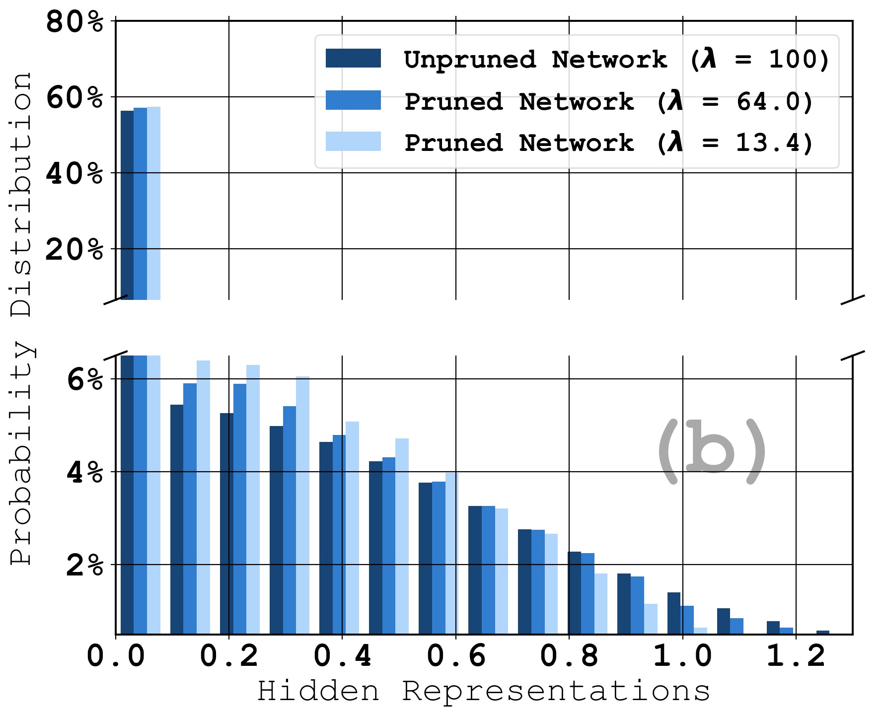
Figure 3: (a) Distribution of weight gradients when iteratively pruning a fully connected ReLU-based network using global magnitude (Han et al. 2015), where $\lambda$ is the percent of weights remaining. (b) Corresponding distribution of hidden representations (i.e., post-activation outputs of all hidden layers). The difference with Fig. 1 is that the batch normalization technique (Ioffe and Szegedy 2015) ($\mu$ = 0, $\sigma^{2}$ = 1) is used here.

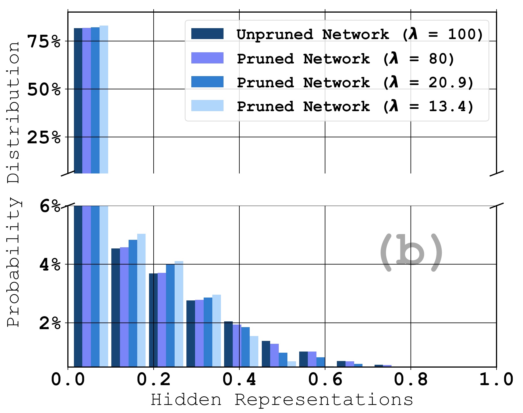
Figure 4: (a) Distribution of weight gradients when iteratively pruning the AlexNet network using the layer magnitude pruning method, where $\lambda$ is the percent of weights remaining. (b) Corresponding distribution of hidden representations (i.e., post-activation outputs of all hidden layers).

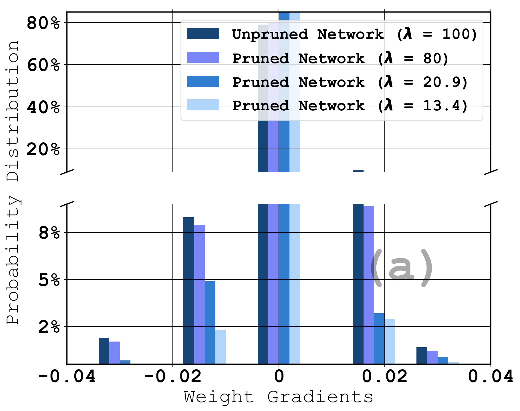
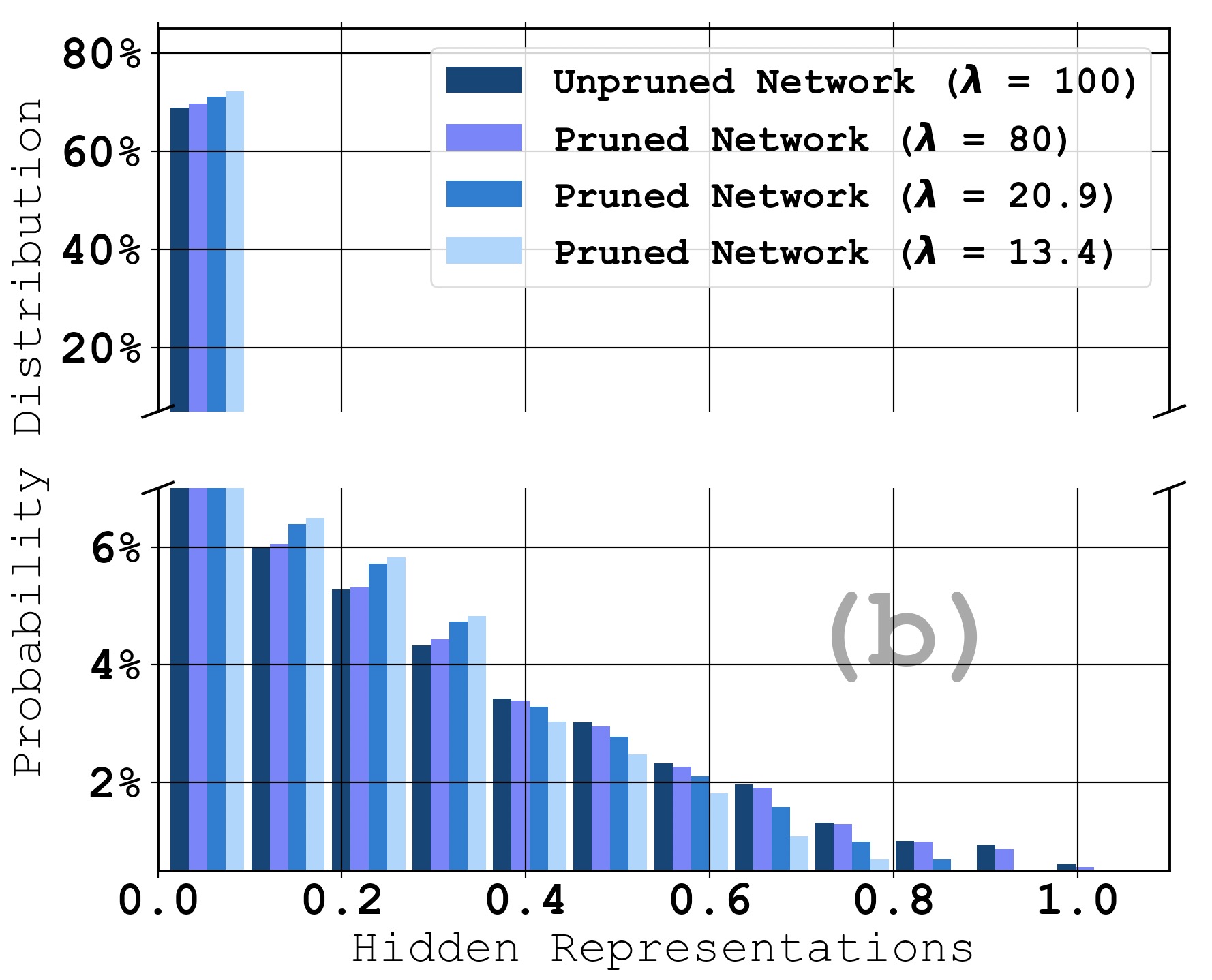
Figure 5: (a) Distribution of weight gradients when iteratively pruning the ResNet-20 network using the global gradient pruning method, where $\lambda$ is the percent of weights remaining. (b) Corresponding distribution of hidden representations (i.e., post-activation outputs of all hidden layers).

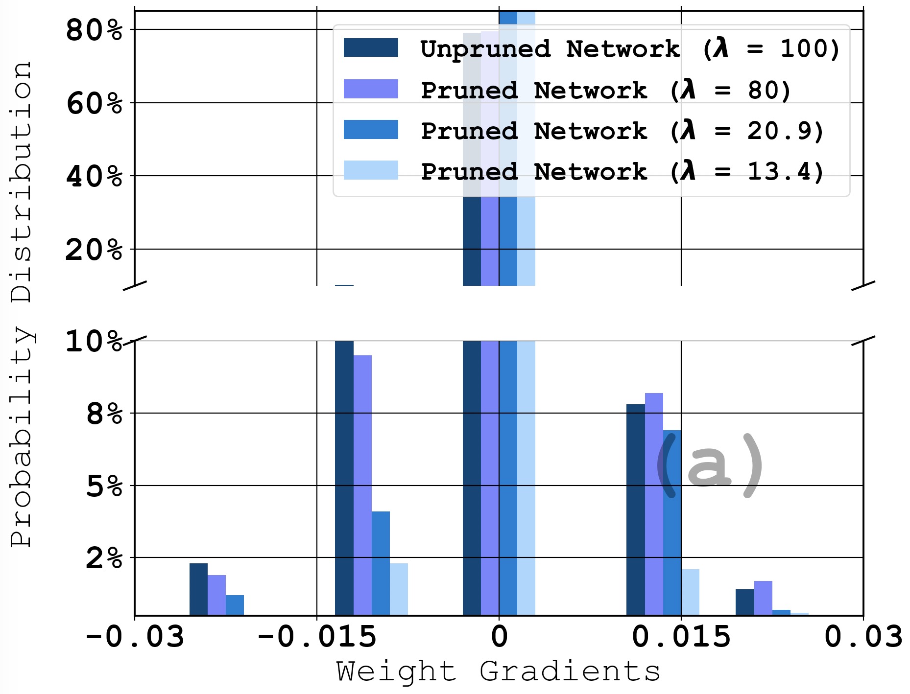
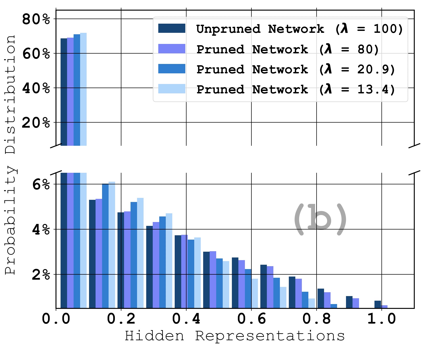
Figure 6: (a) Distribution of weight gradients when iteratively pruning the VGG-16 network using the structured filter pruning method (Li et al. 2017), where $\lambda$ is the percent of weights remaining. (b) Corresponding distribution of hidden representations (i.e., post-activation outputs of all hidden layers).

A.2 Performance Comparison using Adam and RMSProp

In this subsection, we show the performance comparison between the proposed S-Cyc and selected LR benchmarks using Adam (Kingma and Ba 2014) and RMSProp (Tieleman and Hinton 2012) optimizers. The experimental results summarized in Tables 5 - 6 largely mirror those in Table 2. Specifically, the proposed S-Cyc outperforms the best performing benchmark by a range of 0.8% -2.7% in pruned networks.

Params: 227K	Train Steps: 63K Iters	Batch: 128	Batch Norm: Yes	Optimizer: Adam	Rate: 0.2

Percent of Weights Remaining, $\lambda$	100	32.9	21.1	10.9	5.72	2.03
constant LR (8e-4)	88.4$\pm$0.4	84.8$\pm$0.6	83.5$\pm$0.6	80.5$\pm$0.9	75.5$\pm$1.2	67.1$\pm$1.7
LR decay (3e-3, 63K)	88.6$\pm$0.3	87.1$\pm$0.7	83.7$\pm$0.9	82.1$\pm$1.1	76.1$\pm$0.8	66.0$\pm$1.3
cyclical LR (0, 3e-2, 8K)	88.9$\pm$0.3	86.9$\pm$0.5	84.1$\pm$0.3	82.1$\pm$0.5	77.0$\pm$0.9	64.4$\pm$1.1
LR-warmup-1 (3e-3, 20K, 20K, 25K, Nil)	89.1$\pm$0.3	87.2$\pm$0.4	84.5$\pm$0.6	82.6$\pm$0.7	75.2$\pm$1.1	65.1$\pm$1.9
LR-warmup-2 (7e-3, 20K, 20K, 25K, Nil)	87.8$\pm$0.3	85.7$\pm$0.5	84.3$\pm$0.7	82.9$\pm$0.8	78.1$\pm$1.4	69.8$\pm$2.1
S-Cyc (3e-3, 4e-3, 1, 4, 20K, 20K, 25K, Nil)	89.2$\pm$0.2	87.9$\pm$0.3	86.3$\pm$0.5	84.4$\pm$0.6	79.5$\pm$1.7	71.7$\pm$2.3

Table 5: Performance comparison (averaged test accuracy $\pm$ std over 5 runs) of iteratively pruning ResNet-20 on CIFAR-10 dataset using the global weight magnitude pruning method (Han et al. 2015) and the Adam optimizer (Kingma and Ba 2014).

Params: 227K	Train Steps: 63K Iters	Batch: 128	Batch Norm: Yes	Optimizer: RMSProp	Rate: 0.2

Percent of Weights Remaining, $\lambda$	100	32.9	21.1	10.9	5.72	2.03
constant LR (6e-4)	87.9$\pm$0.3	83.4$\pm$0.4	81.5$\pm$0.9	77.0$\pm$0.8	65.5$\pm$1.9	55.1$\pm$2.3
LR decay (2e-3, 63K)	88.4$\pm$0.2	84.8$\pm$0.6	81.3$\pm$1.1	77.8$\pm$0.9	67.1$\pm$1.4	58.3$\pm$1.6
cyclical LR (0, 3e-3, 10K)	88.1$\pm$0.3	84.7$\pm$0.5	81.9$\pm$0.7	78.1$\pm$1.0	67.5$\pm$0.9	56.3$\pm$1.7
LR-warmup-1 (1e-3, 20K, 20K, 25K, Nil)	88.9$\pm$0.2	85.1$\pm$0.5	81.7$\pm$0.4	78.6$\pm$0.6	67.3$\pm$1.3	57.1$\pm$1.4
LR-warmup-2 (3e-3, 20K, 20K, 25K, Nil)	88.5$\pm$0.4	85.8$\pm$0.6	82.6$\pm$0.5	79.9$\pm$0.7	69.3$\pm$1.1	59.2$\pm$2.3
S-Cyc (1e-3, 2e-3, 2, 5, 20K, 20K, 25K, Nil)	88.7$\pm$0.3	86.1$\pm$0.4	83.1$\pm$0.6	81.4$\pm$0.9	72.5$\pm$1.3	63.5$\pm$1.9

Table 6: Performance comparison (averaged test accuracy $\pm$ std over 5 runs) of iteratively pruning ResNet-20 on CIFAR-10 dataset using the global weight magnitude pruning method (Han et al. 2015) and the RMSProp optimizer (Tieleman and Hinton 2012).

A.3 More Experimental Results on Comparing S-Cyc’s max_lr to well-tuned max_lr

we show the performance between S-Cyc’s max_lr to that of an oracle using ResNet-20, global gradient pruning method on CIFAR-10 in Table 7 and ResNet-50, IMP on ImageNet-200 in Table 8. It can be seen that the max_lr estimated by S-Cyc falls in the feasible LR region at each pruning cycle, meaning that the validation accuracy of S-Cyc is comparable to the well-tuned max_lr. This highlights the competitiveness of the proposed S-Cyc using ResNet-20 and ResNet-50.

Percent of Weights Remaining, $\lambda$	100	64	51.3	41.1	32.9	21.1	5.72
Well Tuned max_lr ($\times$e-2)	3.4	3.2	3.8	4.6	5.6	6.2	6.8
Feasible LR Region ($\times$e-2)	[2.8, 3.6]	[3.0, 3.6]	[3.4, 4.2]	[3.8, 5.2]	[5.4, 6.6]	[5.4, 6.8]	[5.8, 7.4]
S-Cyc ($\times$e-2)	3	3	3.2	4.7	6.4	6.9	6.99

Table 7: Comparison between the value of max_lr computed by S-Cyc, well-tuned max_lr via grid search and feasible learning rate region when iteratively pruning the ResNet-20 on the CIFAR-10 dataset using the global weight magnitude pruning method (Han et al. 2015)

Percent of Weights Remaining, $\lambda$	100	64	51.3	41.1	32.9	21.1	5.72
Well Tuned max_lr ($\times$e-2)	4.8	4.6	5.4	5.6	6.8	9.4	9.2
Feasible LR Region ($\times$e-2)	[4.6, 5.0]	[4.6, 5.2]	[4.6, 5.6]	[5.2, 6.0]	[6.6, 7.2]	[9.0, 10.0]	[9.0, 10.2]
S-Cyc ($\times$e-2)	5	5	5	5.2	7.2	9.8	9.9

Table 8: Comparison between the value of max_lr computed by S-Cyc, well-tuned max_lr via grid search and feasible learning rate region when iteratively pruning the ResNet-50 on ImageNet-200 dataset using the IMP pruning method (Le and Yang 2015).

A.4 Experimental Results for More Values of $\lambda$

We note that, in Table 2, we only show the experimental results for some key values of $\lambda$. In this subsection, we show the results for more values of $\lambda$ in Tables 9 - 11. We observe that, for other values of $\lambda$, the proposed S-Cyc still outperforms selected LR benchmarks.

Params: 227K	Train Steps: 63K Iters	Batch: 128	Batch Norm: Yes	Optimizer: SGD	Rate: 0.2

Percent of Weights Remaining, $\lambda$	100	80	64	51.3	41.1	32.9	21.1	10.9	5.72	2.03
constant LR (1e-2)	89.4$\pm$0.4	89.0$\pm$0.4	88.7$\pm$0.5	87.8$\pm$0.7	86.9$\pm$0.9	86.5$\pm$0.9	85.0$\pm$0.7	82.5$\pm$0.3	78.9$\pm$0.8	66.2$\pm$1.3
LR decay (3e-2, 63K)	90.0$\pm$0.4	89.3$\pm$0.2	89.2$\pm$0.3	88.0$\pm$0.5	87.2$\pm$0.6	87.0$\pm$0.8	85.7$\pm$0.6	82.9$\pm$0.6	79.6$\pm$0.7	66.9$\pm$1.9
cyclical LR (0, 3e-2, 8K)	89.6$\pm$0.3	89.2$\pm$0.3	88.7$\pm$0.5	88.2$\pm$0.4	87.7$\pm$0.6	87.2$\pm$0.6	85.6$\pm$0.5	83.0$\pm$0.4	80.1$\pm$0.8	67.8$\pm$1.4
LR-warmup-1 (3e-2, 20K, 20K, 25K, Nil)	90.1$\pm$0.5	89.6$\pm$0.3	89.4$\pm$0.3	88.2$\pm$0.5	87.8$\pm$0.7	87.4$\pm$0.8	85.5$\pm$0.6	83.4$\pm$0.6	80.0$\pm$1.4	68.9$\pm$1.3
LR-warmup-2 (7e-2, 20K, 20K, 25K, Nil)	89.7$\pm$0.4	89.4$\pm$0.2	89.0$\pm$0.5	89.1$\pm$0.4	88.1$\pm$0.6	87.6$\pm$0.5	85.9$\pm$0.4	83.8$\pm$0.8	80.6$\pm$1.2	71.3$\pm$1.2
S-Cyc (3e-2, 4e-2, 1, 5, 20K, 20K, 25K, Nil)	90.0$\pm$0.3	89.6$\pm$0.4	89.3$\pm$0.5	89.2$\pm$0.6	88.3$\pm$0.4	88.3$\pm$0.4	87.1$\pm$0.5	84.5$\pm$0.8	81.7$\pm$0.9	72.8$\pm$1.6

Table 9: Performance comparison (averaged test accuracy $\pm$ std over 5 runs) of pruning ResNet-20 on CIFAR-10 dataset using the global gradient pruning method (Blalock et al. 2020). LR-warmup-1 is the standard implementation used in (Frankle and Carbin 2019; Frankle et al. 2020).

Params: 139M	Train Steps: 63K Iters	Batch: 128	Batch Norm: Yes	Optimizer: SGD	Rate: 0.9

Percent of Weights Remaining, $\lambda$	100	80	64	51.3	41.1	32.9	21.1	10.9	5.72	2.03
constant LR (8e-3)	92.0$\pm$0.3	91.1$\pm$0.4	90.5$\pm$0.5	89.0$\pm$0.6	88.3$\pm$0.6	87.9$\pm$0.7	85.6$\pm$0.9	80.2$\pm$1.4	70.1$\pm$1.3	40.1$\pm$1.4
LR decay (1e-2, 63K)	92.1$\pm$0.5	91.3$\pm$0.3	91.1$\pm$0.5	89.2$\pm$0.5	88.7$\pm$0.4	88.4$\pm$0.5	86.1$\pm$0.6	80.3$\pm$0.8	69.8$\pm$1.9	40.9$\pm$2.9
cyclical LR (0, 3e-2, 15K)	92.3$\pm$0.6	91.6$\pm$0.4	91.3$\pm$0.6	89.6$\pm$0.4	89.2$\pm$0.5	89.2$\pm$0.4	87.2$\pm$0.8	81.1$\pm$1.3	70.4$\pm$1.6	43.2$\pm$1.9
LR-warmup-1 (1e-1, 10K, 32K, 48K, Nil)	92.2$\pm$0.3	92.0$\pm$0.4	91.3$\pm$0.5	90.6$\pm$0.5	89.6$\pm$0.6	89.4$\pm$0.5	87.5$\pm$0.7	81.7$\pm$1.1	71.5$\pm$1.3	46.6$\pm$2.7
LR-warmup-2 (4e-2, 10K, 32K, 48K, Nil)	92.9$\pm$0.3	92.5$\pm$0.3	92.6$\pm$0.3	91.2$\pm$0.7	90.1$\pm$0.4	89.5$\pm$0.4	87.0$\pm$0.5	81.4$\pm$1.2	70.9$\pm$1.4	45.0$\pm$2.3
S-Cyc (4e-2, 6e-2, 2, 4, 10K, 32K, 48K, Nil)	93.0$\pm$0.4	92.4$\pm$0.2	92.8$\pm$0.4	91.9$\pm$0.6	90.6$\pm$0.5	90.2$\pm$0.7	88.2$\pm$1.4	83.1$\pm$1.1	73.2$\pm$0.9	48.2$\pm$2.1

Table 10: Performance comparison (averaged test accuracy $\pm$ std over 5 runs) of pruning VGG-19 on CIFAR-10 dataset using the layer gradient pruning method (Blalock et al. 2020). LR-warmup-1 is the standard implementation used in (Frankle and Carbin 2019; Frankle et al. 2020; Liu et al. 2019).

Params: 23.8M	Train Steps: 70K Iters	Batch: 128	Batch Norm: Yes	Optimizer: SGD	Rate: 0.9

Percent of Weights Remaining, $\lambda$	100	80	64	51.3	41.1	32.9	21.1	10.9	5.72	2.03
constant LR (1e-2)	56.7$\pm$0.3	56.3$\pm$0.2	55.5$\pm$0.2	55.6$\pm$0.7	55.0$\pm$0.7	54.4$\pm$0.4	52.7$\pm$1.2	50.1$\pm$1.3	46.3$\pm$0.9	43.9$\pm$1.2
LR decay (3e-2, 70K	56.7$\pm$0.2	56.1$\pm$0.4	56.0$\pm$0.4	55.4$\pm$0.4	55.2$\pm$0.5	55.0$\pm$0.5	53.1$\pm$1.0	50.9$\pm$1.2	47.0$\pm$0.7	41.8$\pm$1.4
cyclical LR (0, 5e-2, 20K)	56.6$\pm$0.2	56.4$\pm$0.3	55.8$\pm$0.5	55.7$\pm$0.2	55.8$\pm$0.3	55.4$\pm$0.4	54.3$\pm$0.8	52.2$\pm$1.1	46.0$\pm$1.4	43.3$\pm$1.2
LR-warmup-1 (1e-1, 4K, 23K, 46K, 62K)	57.0$\pm$0.3	57.1$\pm$0.2	56.6$\pm$0.4	56.4$\pm$0.6	56.3$\pm$0.4	56.2$\pm$0.5	56.3$\pm$0.6	53.7$\pm$0.9	49.7$\pm$1.1	47.4$\pm$1.1
LR-warmup-2 (5e-2, 4K, 23K, 46K, 62K)	57.8$\pm$0.3	58.1$\pm$0.3	57.2$\pm$0.5	56.5$\pm$0.3	56.2$\pm$0.5	56.6$\pm$0.4	55.9$\pm$0.4	53.3$\pm$1.0	48.6$\pm$1.0	45.0$\pm$0.9
S-Cyc (5e-2, 5e-2, 2, 5, 4K, 23K, 46K, 62K)	57.6$\pm$0.4	58.1$\pm$0.4	57.9$\pm$0.5	57.5$\pm$0.6	57.9$\pm$0.4	57.1$\pm$0.5	56.4$\pm$0.6	54.4$\pm$1.3	51.0$\pm$1.2	48.9$\pm$1.5

Table 11: Performance comparison (averaged test accuracy $\pm$ standard deviation over 5 runs) of pruning ResNet-50 on ImageNet-200 dataset using the IMP pruning method (Le and Yang 2015). LR-warmup-1 is adapted from the standard implementation used in (Frankle et al. 2020; Renda, Frankle, and Carbin 2020).

References

- Allen-Zhu, Li, and Song (2019) Allen-Zhu, Z.; Li, Y.; and Song, Z. 2019. A Convergence Theory for Deep Learning via Over-Parameterization. In Proceedings of the International Conference on Machine Learning (ICML), volume 97, 242–252.
- An et al. (2017) An, W.; et al. 2017. Exponential decay sine wave learning rate for fast deep neural network training. In 2017 IEEE Visual Communications and Image Processing (VCIP), 1–4. IEEE.
- Arora, Cohen, and Hazan (2018) Arora, S.; Cohen, N.; and Hazan, E. 2018. On the optimization of deep networks: Implicit Acceleration by overparameterization. In Proceedings of the International Conference on Machine Learning (ICML), volume 80, 244–253.
- Bengio (2012) Bengio, Y. 2012. Practical recommendations for gradient-based training of deep architectures. In Neural networks: Tricks of the trade, 437–478. Springer.
- Blalock et al. (2020) Blalock, D.; et al. 2020. What is the State of Neural Network Pruning? arXiv preprint arXiv:2003.03033.
- Denil et al. (2013) Denil, M.; et al. 2013. Predicting parameters in deep learning. In Advances in Neural Information Processing Systems (Neurips), 2148–2156.
- Frankle and Carbin (2019) Frankle, J.; and Carbin, M. 2019. The Lottery Ticket Hypothesis: Finding Sparse, Trainable Neural Networks. In International Conference on Learning Representations (ICLR).
- Frankle et al. (2019) Frankle, J.; et al. 2019. Stabilizing the Lottery Ticket Hypothesis. arXiv preprint arXiv:1903.01611.
- Frankle et al. (2020) Frankle, J.; et al. 2020. Linear Mode Connectivity and the Lottery Ticket Hypothesis. In International Conference on Machine Learning (ICML), 3259–3269.
- Gandikota et al. (2021) Gandikota, V.; et al. 2021. vqsgd: Vector quantized stochastic gradient descent. In International Conference on Artificial Intelligence and Statistics, 2197–2205.
- Ge et al. (2019) Ge, R.; et al. 2019. The step decay schedule: A near optimal, geometrically decaying learning rate procedure for least squares. arXiv preprint arXiv:1904.12838.
- Goodfellow, Bengio, and Courville (2016) Goodfellow, I.; Bengio, Y.; and Courville, A. 2016. Deep learning. MIT press.
- Han, Mao, and Dally (2015) Han, S.; Mao, H.; and Dally, W. J. 2015. Deep compression: Compressing deep neural networks with pruning, trained quantization and huffman coding. arXiv preprint arXiv:1510.00149.
- Han et al. (2015) Han, S.; et al. 2015. Learning both weights and connections for efficient neural network. In Advances in Neural Information Processing Systems (Neurips), 1135–1143.
- Hassibi and Stork (1993) Hassibi, B.; and Stork, D. G. 1993. Second order derivatives for network pruning: Optimal brain surgeon. In Advances in Neural Information Processing Systems (Neurips), 164–171.
- He et al. (2015) He, K.; et al. 2015. Delving deep into rectifiers: Surpassing human-level performance on imagenet classification. In Proceedings of the IEEE international conference on computer vision, 1026–1034.
- He et al. (2016) He, K.; et al. 2016. Deep residual learning for image recognition. In Proceedings of the IEEE Conference on Computer Vision and Pattern Recognition, 770–778.
- He et al. (2019) He, T.; et al. 2019. Bag of tricks for image classification with convolutional neural networks. In Proceedings of the IEEE/CVF Conference on Computer Vision and Pattern Recognition, 558–567.
- Hu et al. (2016) Hu, H.; et al. 2016. Network trimming: A data-driven neuron pruning approach towards efficient deep architectures. arXiv preprint arXiv:1607.03250.
- Ioffe and Szegedy (2015) Ioffe, S.; and Szegedy, C. 2015. Batch normalization: Accelerating deep network training by reducing internal covariate shift. In Proceedings of the International Conference on Machine Learning (ICML), volume 37, 448–456.
- Jentzen et al. (2021) Jentzen, A.; et al. 2021. Strong error analysis for stochastic gradient descent optimization algorithms. IMA Journal of Numerical Analysis, 41(1): 455–492.
- Kingma and Ba (2014) Kingma, D. P.; and Ba, J. 2014. Adam: A Method for Stochastic Optimization. arXiv:1412.6980.
- Krizhevsky and Hinton (2010) Krizhevsky, A.; and Hinton, G. 2010. Convolutional deep belief networks on cifar-10. Unpublished manuscript, 40(7): 1–9.
- Krizhevsky et al. (2009) Krizhevsky, A.; et al. 2009. Learning multiple layers of features from tiny images.
- Le and Yang (2015) Le, Y.; and Yang, X. 2015. Tiny imagenet visual recognition challenge. CS 231N.
- LeCun, Denker, and Solla (1990) LeCun, Y.; Denker, J. S.; and Solla, S. A. 1990. Optimal brain damage. In Advances in Neural Information Processing Systems (Neurips), 598–605.
- Lee et al. (2018) Lee, N.; et al. 2018. SNIP: Single-shot network pruning based on connection sensitivity. arXiv preprint arXiv:1810.02340.
- Li et al. (2017) Li, H.; et al. 2017. Pruning filters for efficient convnets. In International Conference on Learning Representations.
- Lin et al. (2020) Lin, M.; Ji, R.; Wang, Y.; Zhang, Y.; Zhang, B.; Tian, Y.; and Shao, L. 2020. Hrank: Filter pruning using high-rank feature map. In Proceedings of the IEEE/CVF Conference on Computer Vision and Pattern Recognition, 1529–1538.
- Liu, Simonyan, and Yang (2018) Liu, H.; Simonyan, K.; and Yang, Y. 2018. DARTS: Differentiable architecture search. arXiv preprint arXiv:1806.09055.
- Liu et al. (2019) Liu, Z.; et al. 2019. Rethinking the value of network pruning. In International Conference on Learning Representations (ICLR).
- Luo and Wu (2020) Luo, J.-H.; and Wu, J. 2020. Neural Network Pruning with Residual-Connections and Limited-Data. In Proceedings of the IEEE/CVF Conference on Computer Vision and Pattern Recognition, 1458–1467.
- Luo, Wu, and Lin (2017) Luo, J.-H.; Wu, J.; and Lin, W. 2017. Thinet: A filter level pruning method for deep neural network compression. In Proceedings of the IEEE International Conference on Computer Vision, 5058–5066.
- Malach et al. (2020) Malach, E.; et al. 2020. Proving the lottery ticket hypothesis: Pruning is all you need. In International Conference on Machine Learning (ICML), 6682–6691.
- Mehta (2019) Mehta, R. 2019. Sparse Transfer Learning via Winning Lottery Tickets. arXiv preprint arXiv:1905.07785.
- Molchanov et al. (2017) Molchanov, P.; et al. 2017. Pruning convolutional neural networks for resource efficient inference. International Conference on Learning Representations (ICLR).
- Molchanov et al. (2019) Molchanov, P.; et al. 2019. Importance estimation for neural network pruning. In Proceedings of the IEEE Conference on Computer Vision and Pattern Recognition, 11264–11272.
- Renda, Frankle, and Carbin (2020) Renda, A.; Frankle, J.; and Carbin, M. 2020. Comparing rewinding and fine-tuning in neural network pruning. arXiv preprint arXiv:2003.02389.
- Ruder (2016) Ruder, S. 2016. An overview of gradient descent optimization algorithms. arXiv preprint arXiv:1609.04747.
- Simonyan and Zisserman (2014) Simonyan, K.; and Zisserman, A. 2014. Very deep convolutional networks for large-scale image recognition. arXiv preprint arXiv:1409.1556.
- Smith (2017) Smith, L. N. 2017. Cyclical learning rates for training neural networks. In 2017 IEEE Winter Conference on Applications of Computer Vision (WACV), 464–472. IEEE.
- Tan and Motani (2020) Tan, C. M. J.; and Motani, M. 2020. DropNet: Reducing Neural Network Complexity via Iterative Pruning. In International Conference on Machine Learning (ICML), 9356–9366. PMLR.
- Tanaka et al. (2020) Tanaka, H.; et al. 2020. Pruning neural networks without any data by iteratively conserving synaptic flow. arXiv preprint arXiv:2006.05467.
- Theis et al. (2018) Theis, L.; et al. 2018. Faster gaze prediction with dense networks and fisher pruning. arXiv preprint arXiv:1801.05787.
- Tieleman and Hinton (2012) Tieleman, T.; and Hinton, G. 2012. Lecture 6.5-rmsprop: Divide the gradient by a running average of its recent magnitude. COURSERA: Neural networks for machine learning, 4(2): 26–31.
- Wang et al. (2020a) Wang, T.; et al. 2020a. APQ: Joint Search for Network Architecture, Pruning and Quantization Policy. In Proceedings of the IEEE/CVF Conference on Computer Vision and Pattern Recognition (CVPR).
- Wang et al. (2020b) Wang, Y.; et al. 2020b. Dynamic Network Pruning with Interpretable Layerwise Channel Selection. In Proceedings of the AAAI Conference on Artificial Intelligence, volume 34, 6299–6306.
- Wang et al. (2020c) Wang, Y.; et al. 2020c. Pruning from scratch. In Proceedings of the AAAI Conference on Artificial Intelligence, volume 34, 12273–12280.
- Xiao, Wang, and Rajasekaran (2019) Xiao, X.; Wang, Z.; and Rajasekaran, S. 2019. AutoPrune: Automatic Network Pruning by Regularizing Auxiliary Parameters. In Advances in Neural Information Processing Systems (Neurips), 13681–13691.
- Yang et al. (2019) Yang, H.; et al. 2019. Filter Pruning via Geometric Median for Deep Convolutional Neural Networks Acceleration. In IEEE Conference on Computer Vision and Pattern Recognition, 4335–4344.
- Ye et al. (2020) Ye, M.; et al. 2020. Good subnetworks provably exist: Pruning via greedy forward selection. In International Conference on Machine Learning (ICML), 10820–10830. PMLR.
- Yeom et al. (2021) Yeom, S.-K.; et al. 2021. Pruning by explaining: A novel criterion for deep neural network pruning. Pattern Recognition, 1078–1099.
- You et al. (2019) You, K.; Long, M.; Wang, J.; and Jordan, M. I. 2019. How does learning rate decay help modern neural networks? arXiv preprint arXiv:1908.01878.
- Yu et al. (2019) Yu, H.; et al. 2019. Playing the lottery with rewards and multiple languages: lottery tickets in RL and NLP. arXiv preprint arXiv:1906.02768.
- Yu et al. (2018) Yu, R.; et al. 2018. Nisp: Pruning networks using neuron importance score propagation. In Proceedings of the IEEE Conference on Computer Vision and Pattern Recognition, 9194–9203.
- Zeiler (2012) Zeiler, M. D. 2012. Adadelta: an adaptive learning rate method. arXiv preprint arXiv:1212.5701.
- Zhou et al. (2019) Zhou, H.; et al. 2019. Deconstructing Lottery Tickets: Zeros, Signs, and the Supermask. In Advances in Neural Information Processing Systems.
- Zhu and Gupta (2018) Zhu, M.; and Gupta, S. 2018. To prune, or not to prune: exploring the efficacy of pruning for model compression. In International Conference on Learning Representations (ICLR).